a field guide for assessing and monitoring reduced forest degradation and carbon
TRANSCRIPT
RRReeessseeeaaarrrccchhh ppprrrooojjjeeecccttt “““KKKyyyoootttooo::: TTThhhiiinnnkkk GGGlllooobbbaaalll,,, AAAcccttt LLLooocccaaalll”””
AAA FFFiiieeelllddd GGGuuuiiidddeee fffooorrr AAAsssssseeessssssiiinnnggg aaannnddd MMMooonnniiitttooorrriiinnnggg
RRReeeddduuuccceeeddd FFFooorrreeesssttt DDDeeegggrrraaadddaaatttiiiooonnn aaannnddd CCCaaarrrbbbooonnn SSSeeeqqquuueeessstttrrraaatttiiiooonnn bbbyyy
LLLooocccaaalll CCCooommmmmmuuunnniiitttiiieeesss
PPPaaarrrttt 111::: fffooorrr cccooommmmmmuuunnniiitttiiieeesss PPPaaarrrttt 222::: fffooorrr tttrrraaaiiinnneeerrrsss PPPaaarrrttt 333::: fffooorrr pppooollliiicccyyy mmmaaakkkeeerrrsss
2009

2
Verplanke, J.J. and E. Zahabu, Eds. 2009: A Field Guide for Assessing and Monitoring Reduced Forest Degradation and Carbon Sequestration by Local Communities. 93 p. Available online from www.communitycarbonforestry.org
This work is licensed under the Creative Commons Attribution-Noncommercial-No Derivative Works 3.0 Netherlands License. To view a copy of this license, visit http://creativecommons.org/licenses/by-nc-nd/3.0/nl/ Project team KYOTO: Think Global, Act Local (K:TGAL) Department of Technology and Sustainable Development University of Twente P.O. Box 217 7500 AE Enschede The Netherlands Telephone: +31 (0)53 489 3545 Fax: +31 (0)53 489 3087 www.communitycarbonforestry.org

3
Table of Contents Part 1: for communities ...................................................................... 1 1. Introduction ............................................................................... 5 2. What to use? .............................................................................. 7
2.1 Forest Measurements ............................................................... 7 2.2 Mobile GIS ............................................................................ 9 2.2.1 Getting started with Mobile GIS .............................................. 10 2.2.2 Important settings (optional) ................................................. 11 2.2.3 How to create layers ........................................................... 12 2.2.4 Mapping landmarks and plots ................................................. 13 2.2.5 Mapping roads .................................................................. 13 2.2.6 Mapping forest areas and complete boundaries ........................... 15
3. Main steps for carbon assessment worked out ..................................... 17
3.1 Forest mapping and stratification .............................................. 17 3.2 Pilot survey to calculate variance .............................................. 17 3.3 Locating permanent sample plots .............................................. 19 3.4 Take measurements from permanent sample plots .......................... 19
4. Analysis and reporting ................................................................. 21
4.1 Data analysis ....................................................................... 21 4.2 Reporting of carbon data ........................................................ 21
Part 2: for trainers .......................................................................... 23 Part 3: for policy makers ................................................................... 57 Appendix 1 Sampling plot data collection form ......................................... 77 Appendix 2 The calculation of the coefficient of variation of tree basal area ..... 79 Appendix 3 Proposed Equipment Configuration ......................................... 81 Appendix 4 Glossary of Carbon Forestry terminology .................................. 83 Appendix 5 Glossary of Mobile GIS terminology ......................................... 87

4

5
1. Introduction
Most community forest management in developing countries involves management of natural forests that would otherwise be degraded or deforested and producing carbon emissions. When communities participate in forest management in forests in their vicinity, they generally halt or reduce the rate of deforestation and degradation, and they allow the forest to regenerate, which enhances the forest sink. This type of forest management is not credited under the current carbon payment mechanisms of the Kyoto Protocol (CDM). Under new policy currently in discussion by the Parties to the UNFCCC, called Reduced Emissions from Deforestation and forest Degradation (REDD), it is possible that community forest management could earn carbon credits. REDD policy would operate on the basis of overall national efforts to slow down loss of carbon from forests. With this mechanism the community managed forests projects could contribute to efforts under the forestry sector to form a country level REDD approach. It is probable that individual projects within the country would then be credited by the country’s government depending on their mitigation levels in the commitment period. This requires that from the start of the project, monitoring is done to determine the standing stock in both the managed project area and unmanaged forests with similar conditions. At any accounting time the difference between the carbon emissions or removals from the without-project activities and the carbon emissions or removals for with-project activities represent the carbon value to be credited. This includes two processes: reduced degradation and forest enhancement i.e. CO2 sequestration. The fundamental requirement for any forestry project to participate in REDD policy is therefore to demonstrate its reduced levels of degradation and increased sequestration. Data for this can, in principle, be obtained through comparing a time series of forest inventories. However, in almost all developing countries, there is no data on forest stock over time because forest inventories have not been carried out systematically. The reason for this is that inventories place heavy demands on forest staff capacity and financial resources. This field guide provides an alternative approach involving local communities in the measurements. Despite the fact that these local people have no formal education in forestry, it is possible to train them to follow the same standard forest inventory protocols as are used by professionals, resulting in data which is as reliable as that produced by professionals. Local people moreover can utilise their indigenous knowledge to collect required forest inventory data, and the inventory can be carried out at low cost compared to one carried out by professional foresters. Since 2003, the Kyoto: Think Global Act Local (K:TGAL) research project has developed and tested procedures and techniques for carbon assessment and monitoring by local communities. The project works with local NGOs and research institutes in Mali, Senegal, Guinea Bissau, Papua New Guinea, Tanzania, Nepal and Uttaranchal (India). The procedures and techniques were tested for different forest types in these countries and this field guide draws experiences from all these countries. Note to the reader This field guide is written in three volumes. Each volume contains similar information but aims towards a different audience. The field guide gives a step-by-step guidance to the procedures and techniques that need to be undertaken at field level. This Part One of the field guide is aimed at the local forest communities that should do the actual carbon assessment and monitoring. It explains the methodology and tool operation in a practical and simple way for people with a more limited understanding of English and who have less knowledge and understanding

6
of the tools. The guide aims at people that are already involved in community forest management. Part Two of the field guide is aimed at trainers that assist local communities to do their own forest carbon measurement and monitoring. This guide gives all the technical details to perform the carbon assessment with recommended tools. Trainers are most likely from local NGOs or CBOs that have experience with community participation and forestry. Part Three of the field guide is written for people who have a general understanding of forestry and carbon assessment. It is intended for policy makers and interested professionals who wish to understand how the local communities (i.e. a team of community members and staff from a local supporting organization) are trained to implement this methodology of carbon assessment using standard procedures. It is also a guide for policy and decision-makers who need to deal with the community carbon assessment and monitoring output. The guide gives insight into the methodology and community output in relation to national and international carbon policies and treaties.

7
2. What to use? Many tools exist that can be used by communities to measure and monitor the state of their forest resources. This field guide shows some of the most common tools to use for measurement and also introduces a mobile system to record and possibly report these measurements electronically. This chapter provides a summary of the tools and some technical issues that the users are exposed to in part one and two of this guide. 2.1 Forest Measurements We measure most common standing tree variables i.e diameter at breast height (Dbh in cm) and total tree height (m). Ordinary forest inventory equipment are recommended (Fig. 1). In part two of this guide it is described in detail how the equipment can be used to measure these variables.
A tree caliper for measuring dbh
A tape to measure tree dbh and sample plot size
Hypsometer for tree height measurement
An extendable pole for height measurement
Fig. 1. Tools for tree measurements
2.1.1 Basic Dbh measurement techniques Tree diameter at breast height (Dbh) is measured at 1.3 m from the ground. Figure 2 gives an example of the pictorials used to instruct the measurement of tree Dbh for trees with normal and irregular shapes.

8
Fig. 2. Example of pictorials to illustrate measurement techniques for trees dbh
1.3 m
1.3 m
1.3 m 1.3 m
1.3 m 1.3 m
1.3 m 1.3 m
Flat terrain Normal or regular tree Measure dbh at 1.3 m
Sloping terrain Normal or regular tree
Measure dbh at 1.3 m on the up-hill side
Leaning trees The 1.3 m length has to be measured parallel to the tree, not vertically. The measured section has
to be perpendicular to the axis of the tree not horizontal Flat terrain
Measure dbh at 1.3 m from the upper side of
the lean
Slopping terrain Measure dbh at 1.3 m
from the upper hill side
Trees with buttresses or aerial roots higher than 1.3 m Measure dbh above buttresses or aerial roots
Forked trees below 1.3 m Consider these as two trees.
Take two separate measurements
9
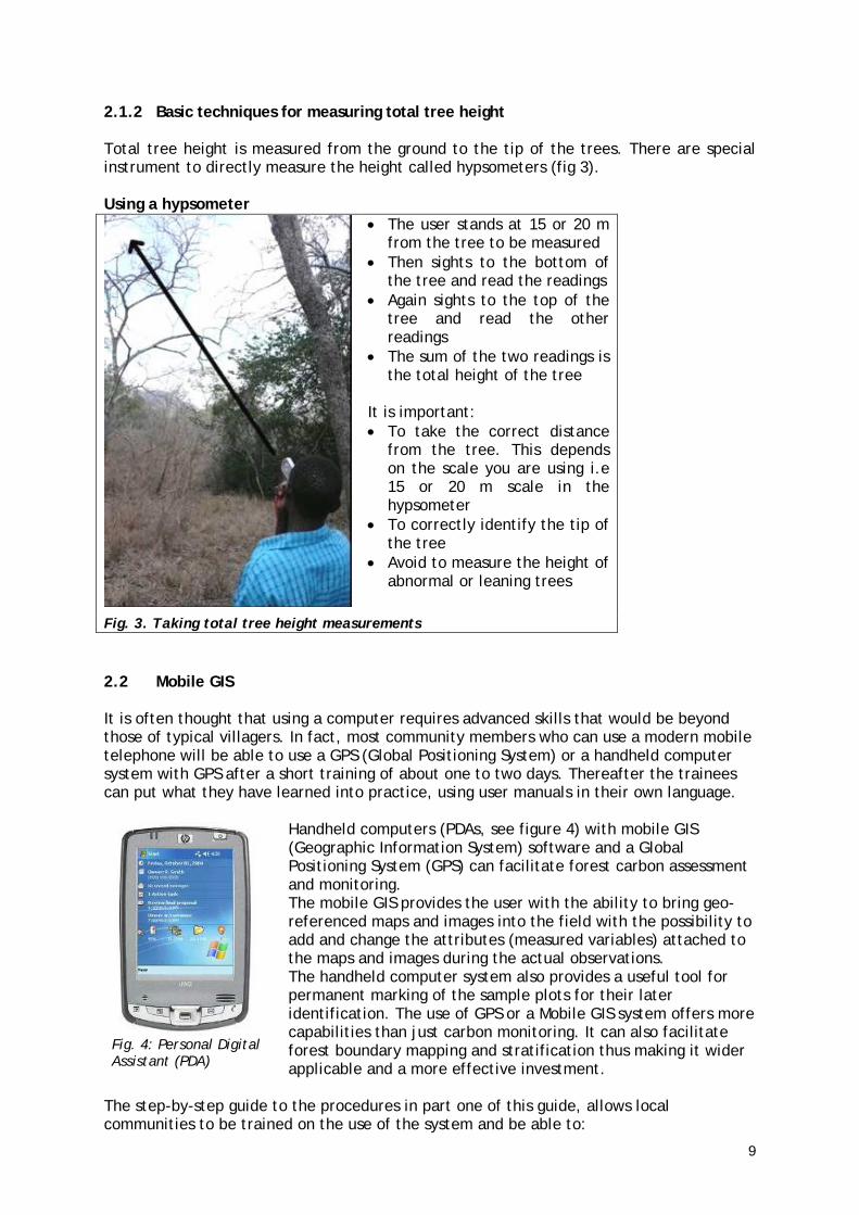
2.1.2 Basic techniques for measuring total tree height Total tree height is measured from the ground to the tip of the trees. There are special instrument to directly measure the height called hypsometers (fig 3). Using a hypsometer
• The user stands at 15 or 20 m from the tree to be measured
• Then sights to the bottom of the tree and read the readings
• Again sights to the top of the tree and read the other readings
• The sum of the two readings is the total height of the tree
It is important: • To take the correct distance
from the tree. This depends on the scale you are using i.e 15 or 20 m scale in the hypsometer
• To correctly identify the tip of the tree
• Avoid to measure the height of abnormal or leaning trees
Fig. 3. Taking total tree height measurements 2.2 Mobile GIS It is often thought that using a computer requires advanced skills that would be beyond those of typical villagers. In fact, most community members who can use a modern mobile telephone will be able to use a GPS (Global Positioning System) or a handheld computer system with GPS after a short training of about one to two days. Thereafter the trainees can put what they have learned into practice, using user manuals in their own language.
Handheld computers (PDAs, see figure 4) with mobile GIS (Geographic Information System) software and a Global Positioning System (GPS) can facilitate forest carbon assessment and monitoring. The mobile GIS provides the user with the ability to bring geo-referenced maps and images into the field with the possibility to add and change the attributes (measured variables) attached to the maps and images during the actual observations. The handheld computer system also provides a useful tool for permanent marking of the sample plots for their later identification. The use of GPS or a Mobile GIS system offers more capabilities than just carbon monitoring. It can also facilitate forest boundary mapping and stratification thus making it wider applicable and a more effective investment.
The step-by-step guide to the procedures in part one of this guide, allows local communities to be trained on the use of the system and be able to:
Fig. 4: Personal Digital Assistant (PDA)

10
map their forest reserves rapidly and with precision and, locate permanent sample plots with accuracy.
In part one of this guide practical tips are provided for dealing with common errors and explanations are given how to basically set-up the mobile equipment. The operational steps assume that there is a local technician available to do the advanced set-up of the equipment so users only need to perform operational sequences and steps. When community members however, gain more skills they can use the guide also to set-up the equipment without support as part one and two provide easy pictorials to guide the user through the necessary steps. 2.2.1 Getting started with Mobile GIS
Switch on the small computer (the PDA) Tap Start - Programs - ArcPad to start the ArcPad program (figure 5) Tap the “Open Map” button (figure 6) on the main toolbar to display the maps available on the PDA Tap on the appropriate map file ( …….. .apm) Your map will now appear on the screen of the computer. Open the Layers menu Before you continue you must make sure that the right map “layer” is activated and can be edited. Each layer that must be edited should first be activated (figure 7) If the box below the Pencil icon is checked this is true. Beware that only one layer of one type (plot’s or landmarks [points]/roads [lines] / boundary [area]) can be activated at once. When the necessary layers can be edited you can go into the field. The next step will be to activate the GPS and this must be done outside (also see “things to know about GPS”). Activate the GPS by tapping the “GPS button” (figure 8). Tap “yes” if a dialog appears to activate the GPS. The “GPS position window” (figure 9) will appear on screen. Wait until the screen develops and “3D” appears in the window. This can take 1 to 10 minutes. When this is done, within the circles you see now numbers representing the satellites in the sky above. (figure 9). If “2D” remains indicated after several minutes try to find a location op open ground to receive a GPS signal (see also the section on “things to know about GPS”). In case there is no signal or a signal “Alert” appears (figure 10) it is important to check the GPS connection (see also section 3.1.2). Alerts can indicate that there is no connection or no signal. In case the system operates with an external GPS please refer to the section: “Things to know about GPS” in Part 2 of this guide. When “3D” is shown (figure 9) and “PDOP” is smaller than “15.0” you are ready to navigate.
Fig. 5: Select program to activate
Fig. 6: ArcPad window
Fig 7: Activate data layers
Fig. 8: activating the GPS
Fig. 9: the GPS position window

11
Turn the PDA off and move to the starting point of data collection. At the starting point, activate both PDA and GPS again and start mapping.
Fig. 10: GPS signal Alerts
2.2.2 Important settings (optional)
Before you can use ArcPad to map your plots and forest areas a few settings need to be checked. The most important one is the connection with your Global Positioning System (GPS). On the ArcPad toolbar you can access the GPS settings menu by tapping on the arrow next to the GPS symbol (fig. 11). Select the option “GPS Preferences …”. The Preferences screen that appears (fig. 12) allows you to connect to your GPS. This can be the internal GPS of your PDA, or an external GPS that is connected via cable or BlueTooth® If you turn on your GPS and then tap on the “binoculars” symbol, the programme will automatically search for and connect with your GPS. In the preferences menu you can also make various other changes to the settings. Please do not make any changes that are not described in this guide. Making changes to the [Alerts] section (fig 13) is not harmful. These alerts notify you if you have lost connection or signal of the GPS. Other settings can be changed under the “Tools” menu (fig. 14) where you can select “Options …”. These options are referering to general programme settings. In principle the default settings are good for your mapping exercise and you do not need to make any changes here. For each layer you use in your map there are also settings that can be changed. If you open the “Table of Contents” menu (fig. 15) a list of available layers in your map will appear. By tapping on the title of a layer the settings menu for this layer will appear. There you can change symbols and colours in your layer. If you open the “map properties” on the right sidebar you can access the properties of your map.
Fig. 11: GPS Settings
Fig. 12: Finding the GPS
Fig. 13: GPS Alerts
Fig. 14: ArcPad settings
Fig. 15: Layer settings
12
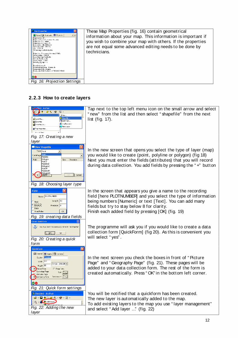
These Map Properties (fig. 16) contain geometrical information about your map. This information is important if you wish to combine your map with others. If the properties are not equal some advanced editing needs to be done by technicians.
Fig. 16: Projection Settings 2.2.3 How to create layers
Tap next to the top left menu icon on the small arrow and select “new” from the list and then select “shapefile” from the next list (fig. 17). In the new screen that opens you select the type of layer (map) you would like to create (point, polyline or polygon) (fig 18) Next you must enter the fields (attributes) that you will record during data collection. You add fields by pressing the “+” button In the screen that appears you give a name to the recording field [here PLOTNUMBER] and you select the type of information being numbers [Numeric] or text [Text]. You can add many fields but try to stay below 8 for clarity. Finish each added field by pressing [OK] (fig. 19) The programme will ask you if you would like to create a data collection form [QuickForm] (fig 20). As this is convenient you will select “yes”. In the next screen you check the boxes in front of “Picture Page” and “Geography Page” (fig. 21). These pages will be added to your data collection form. The rest of the form is created automatically. Press “OK”in the bottom left corner. You will be notified that a quickform has been created. The new layer is automatically added to the map. To add existing layers to the map you use “layer management” and select “Add layer …” (fig. 22)
Fig. 17: Creating a new layer
Fig. 18: Choosing layer type
Fig. 19: creating data fields
Fig. 20: Creating a quick form
Fig. 21: Quick form settings
Fig. 22: Adding the new layer

13
2.2.4 Mapping landmarks and plots
Once you have created the required layers for your mapping project, or when all the layers are made available to you, you can start recording data. To start mapping plots or landmarks you select a “point layer” from the edit menu [see symbol for Plot.shp in fig. 23]. When you are near the point you wish to map, activate the GPS to record its position (fig. 24). Wait until the GPS window shows “3D” (fig. 25) in which case you have sufficient signal from the GPS to record the location of the point accurately. Your position is now shown on screen (fig. 26) by the yellow cross in the red circle. If you have a map or photo on your screen you can check if the position is correct by orienting yourself by available landmarks that are also on your screen. To record the coordinates of your position you can now press the “capture point” button. This will record the position from the GPS and immediately open the data collection form (fig. 27) Once the form is shown on screen you can start entering the different data (attributes) that are created with this layer. Measure the different items according to the methods described in the forest measurement part of this guide. When you have filled all fields with the required data you press “ok” on the bottom of the form and your information about the point is stored. You can now go to the next point.
Fig. 23: selecting edit layer
Fig. 24: activating the GPS
Fig. 25: acquiring GPS signal
Fig. 26: capturing a point
Fig. 27: entering data
2.2.5 Mapping roads
Besides point locations of for example a plot it is also possible to map so called “line features”. The most common line feature on maps are roads. From the edit menu you select a “line layer” from the edit menu [see symbol for “roads” in fig. 28]. When you are near the start of the road you wish to map, activate the GPS (fig. 24). Wait until the GPS window shows “3D” (fig. 25) in which case you have sufficient signal from the GPS to record the location of the road accurately. From the “edit toolbar” (fig. 29) you open the “feature menu” and select “Polyline” as your feature to map.
Fig. 28: selecting edit layer
Fig. 29: selecting map feature

14
Once you have selected the “Polyline” as mapping feature you can see that on the “edit toolbar” two more buttons are activated (fig. 30) We start with the middle button called “Capture Vertex”. You can use this button to record corners in roads. Each time you change direction on a road you press this button and on your screen a new point appears along your road. This recording mode is convenient if your road is mostly consisting of straight segments (fig. 31). Also if the road is long you can switch off your GPS and PDA to conserve battery power and only activate it when you need to record the next corner in the road. If you record a corner by accident you can “undo” this action by tapping the “undo arrow” on the bottom of the screen (fig. 32) Once you come to the end of the road you can finish your line by tapping the green arrow button on the bottom of the screen (fig. 33). This will open your data collection form. Once the form is shown on screen you can start entering the different data (attributes) that are created with this layer. Fill in the different items that must be recorded. When you have filled all fields you press “ok” on the bottom of the form and your information about the road is stored. It is also possible to record points a long a line continuously. For this you use the third capture button called “Capture Vertices” (fig. 34). From the moment you activate this button the programme will map your position continuously until you press the green arrow button at the bottom of the screen (fig. 35). This mapping method is convenient if you are mapping very much winding roads or at high speeds (e.g. from a car). Be aware that recording continues when you are standing still, as each second your location is computed. GPS errors can then be recorded as movement (position shift of 10 to 50 meters) and lead to strange corners in your road.
Fig. 30: Capturing vertices
Fig. 31: Mapping straight lines
Fig. 32: Undo action
Fig. 33: Finish mapping
Fig. 34: data collection form
Fig. 35: recording continuously

15
2.2.6 Mapping forest areas and complete boundaries It is also possible to map so called “area features”. These are areas or “polygons” that are fully enclosed by one or more lines. These could be boundaries that are defining the extent of the forest area or different forest strata. From the edit menu you select a “polygon layer” from the edit menu [see symbol for “areas” in fig. 36]. From the “edit toolbar” (fig. 37) you open the “feature menu” and select “Polygon” as your feature to map. When you are near the start of the road you wish to map, activate the GPS (fig. 24). Wait until the GPS window shows “3D” (fig. 43) in which case you have sufficient signal from the GPS to record the location of the road accurately. Once you have selected the “Polygon” as mapping feature you can see that again on the “edit toolbar” two more buttons are activated (fig. 30) Forest boundary mapping can as with roads be done by mapping straight lines between boundary markers. By marking these markers on an area (polygon) layer the boundary of the area will be drawn on screen while mapping (in fig. 38 this is done using the “capture vertex” option). On closing the area (pressing the green arrow button), when reaching the starting point again, the data corresponding to the area can be entered in the appearing data collection form and afterwards a filled “polygon” will appear on screen. The data collection form of this polygon also contains the surface area (see fig. 38; tap the “geography” tab to see this). Using the “capture vertex” option is advisable as it allows the GPS and PDA to be turned off between distant points. This saves battery power and allows the survey the liberty to follow accessible paths between known points. Sometimes if the boundary is not made up of straight sections between points but curved or uneven sections which require rather exact recording. These can be mapped like the roads in section 3.1.5 using the “capture vertices” option (fig. 39).
Fig. 36: Selecting area layer
Fig. 37: Selecting polygon feature
Fig. 38: Mapping areas by vertex
Fig. 39. Mapping points, roads and areas.

16

17
3. Main steps for carbon assessment worked out
The main steps for carbon assessment include: • Forest mapping and stratification, • Pilot survey to calculate variance, • Locating permanent sample plots on the ground, and • Taking measurements from the plots.
3.1 Forest mapping and stratification If the forest map does not exist, it has to be drawn using mobile GIS as shown in Section 2.2.6. Using experiences on the forest, the field group should walk around the forest and divide the forest into strata. Strata being areas which are distinctly different from each other in type and which would have different amount of carbon stored. E.g. heavily degraded forest area, normal forest, age class etc (fig 40). Stratum 1 Stratum 2 Stratum 3
Fig 40. Examples of different strata that can be distinguished in forests. 3.2 Pilot survey to calculate variance For each stratum, team members make a pilot survey to estimate the variance in tree stocking for the determination of the number of plots for the main inventory. Data from at least 15 sample plots distributed over each stratum will required. We recommend the use of nested sample plots (a large circle containing smaller sub-units) and measure small trees in small sub-plots and large trees in the whole area (larger circle). The size of the large outer circle will be decided. An example for a typical plot for the tropical woodlands is given in fig 41.

18
Fig. 41. Shape and size of the plot for tropical woodlands Measurements to be taken from the plot (i) Trees measurements Within 2 m radius measure the Dbh of:
• all trees greater than 1 cm Dbh, Within 5 m radius measure the Dbh of:
• all trees greater than 5 cm Dbh Within 10 m radius:
• all trees greater than 10 cm Dbh; and Within 15 m radius:
• all trees greater than 20 cm Dbh (ii) Total tree height measurement Measure the height of three trees (i.e small, médium and largest). The calculation of sample size required is based on the variability of trees and saplings as measured in the pilot survey. In the pilot survey the herb and grass layers are not sampled. The number of sampling units (n) is calculated using the formula:
Where: CV = is the coefficient of variation which is the measure of variability of
tree cross-sectional area at breast height t = is the expression of confidence that the true average is within the
estimated range. For 15 plots this always has a value of: 2.32. E = is the error that you are willing to accept in the final estimation of
the mean. Example: Given CV of basal area = 40%, t value for the 15 plots = 1.761 and E = 10%
Then n= (0.42 x 1.7612)/0.12 = 50 plots
2
22
EtCVn =
2 m 5 m
10 m
15 m

19
3.3 Locating permanent sample plots The required number of permanent plots is then laid out in each stratum. Plots of the same size as for pilot survey are used. Systematic layout of plots with a random start should be used. First the plots are systematically laid out on the map and secondly on the ground. The result of this process is a combined random and systematic sampling frame, with the advantage that the plots can always be found again if the start points along the chosen boundary are known, as well as the bearings and the distances along the transects to each plot. Actual forest carbon measurement begins when the group meets at the starting point of the first transect. Then a sequence of activities takes place to locate and record starting points and plot centers (fig 42).
(a) Sighting the direction of the transect using a compass,
(b) Measuring distance between plots using a tape measure,
(c) Demarcating a plot using a tape measure (d) Recording details of the description of the plot to
the handheld computer database,
Fig. 42 a-d: Illustrations to show the sequence of activities while locating permanent sample plots on ground 3.4 Take measurements from permanent sample plots Each tree is recorded individually with its local name and botanical name. It is very important that the same trees are measured every year in each plot. For consistency of measurements compare, the measurements in the successive years as shown in Appendix 1. Use similar plots shape, sizes and take the trees measurements as was done during the pilot survey.

20

21
4. Analysis and reporting 4.1 Data analysis From the collected data, forest stand biomass is computed using locally available allometric equations. Details for the computations are given in the Part two of this guide. 4.2 Reporting of carbon data The results will be presented as shown in Table 1. It is not certain whether the payment of carbon will be based on average or minimum estimate. It is more likely that minimum estimate will be used that is why the average values are shown with their lower and upper limits. Table 1: an example for the carbon data reporting
Forest Name KSUATFR
Vegetation type Miombo woodland
Year 2005
Stems ha 694.9±82 (12%)
Volume per ha (m3ha-1) 68.12±16.92 (14%)
Biomass (t ha-1) 42.19±8.65 (9%)
Carbon (t ha-1) 20.39±4.24 (9%)
Mean CO2 t/ha 74.83
Upper limit CO2 t/ha 90.39
Lower limit CO2 t/ha 59.27
The numbers in brackets indicate precision levels of estimates i.e. percentage confidence intervals to average value of estimate.

22

23
RRReeessseeeaaarrrccchhh ppprrrooojjjeeecccttt “““KKKyyyoootttooo::: TTThhhiiinnnkkk GGGlllooobbbaaalll,,, AAAcccttt LLLooocccaaalll”””
AAA FFFiiieeelllddd GGGuuuiiidddeee fffooorrr AAAsssssseeessssssiiinnnggg aaannnddd MMMooonnniiitttooorrriiinnnggg
RRReeeddduuuccceeeddd FFFooorrreeesssttt DDDeeegggrrraaadddaaatttiiiooonnn aaannnddd CCCaaarrrbbbooonnn SSSeeeqqquuueeessstttrrraaatttiiiooonnn bbbyyy
LLLooocccaaalll CCCooommmmmmuuunnniiitttiiieeesss
PPPaaarrrttt 111::: fffooorrr cccooommmmmmuuunnniiitttiiieeesss PPPaaarrrttt 222::: fffooorrr tttrrraaaiiinnneeerrrsss PPPaaarrrttt 333::: fffooorrr pppooollliiicccyyy mmmaaakkkeeerrrsss
2009

24
This work is licensed under the Creative Commons Attribution-Noncommercial-No Derivative Works 3.0 Netherlands License. To view a copy of this license, visit http://creativecommons.org/licenses/by-nc-nd/3.0/nl/ Project team KYOTO: Think Global, Act Local (K:TGAL) Department of Technology and Sustainable Development University of Twente P.O. Box 217 7500 AE Enschede The Netherlands Telephone: +31 (0)53 489 3545 Fax: +31 (0)53 489 3087 www.communitycarbonforestry.org

25
Table of Contents 1. Introduction ............................................................................. 27 2. The project methodology ............................................................. 29 3. What to use? ............................................................................ 31
3.1 Forest Measurements ............................................................. 31 3.2 Mobile GIS .......................................................................... 32
4. How to collect data? ................................................................... 35
4.1 Selection of the local community trainees and training .................... 35 4.2 Getting started with Mobile GIS ................................................ 36 4.3 Training on measurement of forest stock ..................................... 39 4.4 Main steps for carbon assessment .............................................. 41
5. How to analyze and report the data? ................................................ 51
5.1 Data analysis for the trees ....................................................... 51 5.2 Data analysis for non-tree vegetation, litter and soils ...................... 52 5.3 Reporting of carbon data ........................................................ 52
6. How to implement? .................................................................. 55
Organizing and executing training sessions. .......................................... 55 Part 3: for policy makers ................................................................... 57 Appendix 1 - Sampling plot data collection form ....................................... 77 Appendix 2 - The calculation of the coefficient of variation of tree basal area ... 79 Appendix 3 - Proposed Equipment Configuration ....................................... 81 Appendix 4 - Glossary of Carbon Forestry terminology ................................. 83 Appendix 5 - Glossary of Mobile GIS terminology ....................................... 87

26

27
1. Introduction
Most community forest management in developing countries involves management of natural forests that would otherwise be degraded or deforested and producing carbon emissions. When communities participate in forest management in forests in their vicinity, they generally halt or reduce the rate of deforestation and degradation, and they allow the forest to regenerate, which enhances the forest sink. This type of forest management is not credited under the current carbon payment mechanisms of the Kyoto Protocol (CDM). Under new policy currently in discussion by the Parties to the UNFCCC, called Reduced Emissions from Deforestation and forest Degradation (REDD), it is possible that community forest management could earn carbon credits. REDD policy would operate on the basis of overall national efforts to slow down loss of carbon from forests. With this mechanism the community managed forests projects could contribute to efforts under the forestry sector to form a country level REDD approach. It is probable that individual projects within the country would then be credited by the country’s government depending on their mitigation levels in the commitment period. This requires that from the start of the project, monitoring is done to determine the standing stock in both the managed project area and unmanaged forests with similar conditions. At any accounting time the difference between the carbon emissions or removals from the without-project activities and the carbon emissions or removals for with-project activities represent the carbon value to be credited. This includes two processes: reduced degradation and forest enhancement i.e. CO2 sequestration. The fundamental requirement for any forestry project to participate in REDD policy is therefore to demonstrate its reduced levels of degradation and increased sequestration. Data for this can, in principle, be obtained through comparing a time series of forest inventories. However, in almost all developing countries, there is no data on forest stock over time because forest inventories have not been carried out systematically. The reason for this is that inventories place heavy demands on forest staff capacity and financial resources. This field guide provides an alternative approach involving local communities in the measurements. Despite the fact that these local people have no formal education in forestry, it is possible to train them to follow the same standard forest inventory protocols as are used by professionals, resulting in data which is as reliable as that produced by professionals. Local people moreover can utilise their indigenous knowledge to collect required forest inventory data, and the inventory can be carried out at low cost compared to one carried out by professional foresters. Since 2003, the Kyoto: Think Global Act Local (K:TGAL) research project has developed and tested procedures and techniques for carbon assessment and monitoring by local communities. The project works with local NGOs and research institutes in Mali, Senegal, Guinea Bissau, Papua New Guinea, Tanzania, Nepal and Uttaranchal (India). The procedures and techniques were tested for different forest types in these countries and this field guide draws experiences from all these countries. The field guide gives a step-by-step guidance to the procedures and techniques that need to be undertaken at field level. The field guide is intended to be used to train local communities (i.e. a team of community members and staff from a local supporting organization) in the use a standard procedure of carbon assessment. The inventory procedure itself draws heavily on MacDicken (1997), Weyerhaeuser (2000) and on Good Practice Guidance for Land Use, Land-Use Changes and Forestry (Intergovernmental Panel on Climate Change (IPCC), 2003). Elements of these procedures have been adapted and set out in a simple way to meet the needs of non-professional community members.

28
Note to the reader This field guide is written in three volumes. Each volume contains similar information but aims towards a different audience. Part one is a field guide for the local forest communities that should do the actual carbon assessment and monitoring. It explains the methodology and tool operation in a practical and simple way for people with a more limited understanding of English and who have less knowledge and understanding of the tools. The guide aims at people that are already involved in community forest management. Part two of the field guide (this guide) is aimed at trainers that assist local communities to do their own. This guide gives all the technical details to perform the carbon assessment with recommended tools. Trainers are most likely from local NGOs or CBOs that have experience with community participation and forestry. Trainers can use this volume for themselves and use “Part one” as documentation for the community members. Part three is a guide for policy and decision-makers who need to deal with the community carbon assessment and monitoring output. That guide gives insight into the methodology and community output relation to national and international carbon policies and treaties. The third volume is written for people who have a general understanding of forestry and carbon assessment.
29
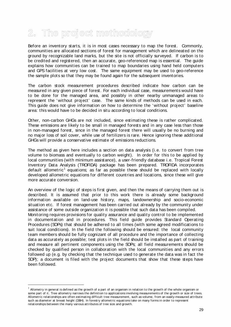
2. The project methodology Before an inventory starts, it is in most cases necessary to map the forest. Commonly, communities are allocated sections of forest for management which are delineated on the ground by recognizable land marks, but the site is not officially surveyed. If carbon is to be credited and registered, then an accurate, geo-referenced map is essential. The guide explains how communities can be trained to map boundaries using hand held computers and GPS facilities at very low cost. The same equipment may be used to geo-reference the sample plots so that they may be found again for the subsequent inventories. The carbon stock measurement procedures described indicate how carbon can be measured in any given piece of forest. For each individual case, measurements would have to be done for the managed area, and possibly in other nearby unmanaged areas to represent the ‘without project’ case. The same kinds of methods can be used in each. This guide does not give information on how to determine the ‘without project’ baseline area: this would have to be decided in situ according to local conditions. Other, non-carbon GHGs are not included, since estimating these is rather complicated. These emissions are likely to be small in managed forests and in any case less than those in non-managed forest, since in the managed forest there will usually be no burning and no major loss of soil cover, while use of fertilizers is rare. Hence ignoring these additional GHGs will provide a conservative estimate of emissions reductions. The method as given here includes a section on data analysis (i.e. to convert from tree volume to biomass and eventually to carbon weight). In order for this to be applied by local communities (with minimum assistance), a user-friendly database i.e. Tropical Forest Inventory Data Analysis (TROFIDA) package has been prepared. TROFIDA incorporates default allometric1
equations; as far as possible these should be replaced with locally developed allometric equations for different countries and locations, since these will give more accurate conversion.
An overview of the logic of steps is first given, and then the means of carrying them out is described. It is assumed that prior to this work there is already some background information available on land-use history, maps, landownership and socio-economic situation etc. If forest management has been carried out already by the community under assistance of some outside organization it is possible that such data has been compiled. Monitoring requires provisions for quality assurance and quality control to be implemented in documentation and in procedures. This field guide provides Standard Operating Procedures (SOPs) that should be adhered to all times (with some agreed modifications to suit local conditions). In the field the following should be ensured: the local community team members should be fully cognizant of all procedure and the importance of collecting data as accurately as possible; test plots in the field should be installed as part of training and measure all pertinent components using the SOPs; all field measurements should be checked by qualified person in collaboration with the local communities and any errors followed up (e.g. by checking that the technique used to generate the data was in fact the SOP); a document is filed with the project documents that show that these steps have been followed.
1 Allometry in general is defined as the growth of a part of an organism in relation to the growth of the whole organism or some part of it. Tree allometry narrows the definition to applications involving measurements of the growth or size of trees. Allometric relationships are often estimating difficult tree measurement, such as volume, from an easily-measured attribute such as diameter at breast height (DBH). In forestry allometric equations take on many forms in order to represent relationships between the many various attributes of tree size and growth.

30
We have been experimenting with this field guide in a number of countries with different forest types, and it is proved to work well in all these cases. However, according to local conditions (density of forest, nature of the terrain etc), local decisions may have to be made to deviate from what we have suggested here. If this is the case, a record should be made of what exactly was done, and why.

31
3. What to use? Many tools exist that can be used by communities to measure and monitor the state of their forest resources. In this field guide we will show some of the most common tools to use for measurement and also introduce a mobile electronic system to record and possibly report these measurements. This chapter provides the tools overview, to choose from, together with some technical issues that the user should take note of when considering the options. In Chapter 4 it is explained in detail how to operate the recommended tools and how to take measurements in the forest. It must be clear from the start that these tools are only recommendations of which some have been tested under different conditions and those test results are reflected in this guide. Specially with respect to the use of “mobile GIS” care must be taken that the use of such a tools is first of all worth the effort and investment and secondly proper to the situation. Many of the tools described in this guide are relatively expensive and can only be justified if a good return is expected. Most importantly the chosen tools should be practical and useful in the field according to the local situation. Community members that actually do the measurements should be (made) comfortable with the chosen tools. Going for a high-end or most advanced option will not always be the most appropriate. In the case of mobile GIS one should always consider that a paper notebook with a pencil has for centuries been known as a good alternative for recording data. 3.1 Forest Measurements The most common standing tree variables used in assessing biomassare dbh (diameter at breast height) and total tree height. Dbh may be measured using calipers or tapes while height is measured using hypsometers or poles (Figure 3). Calipers are normally made of wood, steel or aluminium. Aluminium calipers are more convenient because they are light and durable. Often a single caliper measurement is adequate. However for an elliptical cross section of a stem, two caliper readings at right angles should be made and the average recorded. To obtain reliable measurements, operators must be trained to ensure that:- - the point of measurement is located correctly (it is recommended to use a stick of
1.3m consistently whenever dbh is measured) - the place of the calipers is at right angles to the longitudinal axis of the tree - the correct pressure is applied at the moment of measurement - the bar of the caliper is pressed against the stem. The diameter tape actually measures the circumference of the stem. The diameter graduations are based on the relationship between diameter and circumference. Often diameter measurements with the tape are more consistent than using a caliper provided the tape is level and pulled tightly at the time of measurement. Calipers are convenient for measuring trees up to 50 cm diameter. Diameter tapes are preferred for larger trees because large calipers are bulky and inconvenient to handle. Measuring elliptical stems with the tape however tends to overestimate diameter in which case a caliper is preferable. Instruments for measuring height are known as hypsometers. Common hypsometers include the trigonometric instruments based on angles such as Suuto hypsometer and Haga altimeter. Poles can also me used to measure tree heights (Figure 1)

32
A tree caliper for measuring dbh
A tape to measure tree dbh and sample plot size
Hypsometer for tree height measurement
An extendable pole for height measurement
Fig. 1. Tools for tree measurements
3.2 Mobile GIS The use of GPS or hand held computer system with Geo-Information System (GIS) software (Mobile GIS system) facilitates the forest boundary mapping and stratification. The hand held computer system also provides a useful tool for permanent marking of the sample plots for their later identification. It is often thought that using a computer requires advanced skills that would be beyond those of typical villagers. In fact, any community member who can use a mobile telephone will be able to use a GPS and handheld computer system after a short training of about one to two days. Thereafter, for a week, the trainees need to put what they have learned into practice, using user manuals in their own language. Hand held computers (PDAs) with ArcPad™ software and a Global Positioning System (GPS) can facilitate forests carbon assessment and monitoring. The mobile GIS provides the user

33
with the ability to bring geo-referenced maps and images into the field with the possibility to add and change the attributes attached to the maps and images during the actual observations. It offers users the ability to connect a GPS to the hand held computer. PDA’s are commonly manufactured to include a GPS receiver or connect to an external GPS receiver through Bluetooth. This way a position on ground can be shown in real time on a map on the PDA screen. With this system it is possible very simply to locate forestry boundary and sample plots. The system tested included a PDA/Pocket PC handheld computer (windows mobile operating system) with integrated GPS and ArcPad software. It is expected that, with a step-by-step guide to the procedures, local communities can be trained on the use of the system and be able to: map their forest reserves rapidly and with precision and, locate permanent sampling plots with accuracy.
Things to know about the PDA A PDA is a very small computer (can be as small as a cell phone, figure 2) that can perform many tasks as any Desktop PC or Laptop. Its limitations lie with its computing power and
data storage capacity. A PDA does not always come with a keyboard. As a pointing device a “Stylus” is used to operate screen buttons and to type on the on-screen keyboard. The Stylus can also be used to write on the PDA screen as PDA’s can understand handwriting. It is designed to function together as a pair with a Desktop PC or Laptop, creating a functional tool that enables the user to take computer files into the field to update or append. PDA’s can only be operated if an AC power source is available every 48-72 hours. It needs regular charging of its battery. Operating time of a PDA can vary between 4 to 16 hours, depending on the tasks required. If battery power is depleted for too long the PDA needs to be reinitiated while connected to its “paired” Desktop or Laptop. To prevent data loss in such an event it is recommended to store all data and make backups on memory cards. These cards (most commonly “SD-cards”) fit in an external slot and can be
exchanged when needed. Usually a memory card of 1GB will be more than sufficient to use in data collection exercises. A PDA can be switched off (standby) at any moment to save battery power. It operates in such a way that each time the power is turned on it will recommence at the point/program where it was turned off. Particularly if data is not collected continuously it is strongly recommended to switch the device to standby whenever possible. See Appendix 3 for the proposed equipment configurations and costs estimations. Before using the PDA and ArcPad The ArcPad software should be installed on the PDA when community members start to use it. If not then a qualified person should perform this operation first. Usually there exists a backup of all software on the storage memory of the PDA. This can be used to restore all programmes in case of power loss. If ArcPad is not installed the following guide can be followed: Before working with a mobile GIS system one must make sure that all parts of the system can communicate with each other. The system works initially from a desktop or laptop computer. Firstly a software package must be installed on this computer to communicate with and to transfer date to the PDA. For Wndows based devices, the software to use is Microsoft ActiveSync which is usually supplied together with the PDA. Follow the instructions provided with the software to install this package. It is crucial that this
Fig. 2: Personal Digital Assistant (PDA) or Pocket PC

34
software is installed before any other Mobile Software (for the PDA) is installed on the desktop/laptop computer. Once ActiveSync is installed, a connection can be made with a PDA and after this, software (such as ArcPad) can be installed (see ActiveSync installation manual). Things to know about GPS A Global Positioning System (GPS) works like a radio, receiving signals from 24 satellites in orbit around our planet. When a GPS unit on the ground receives 4 or more of these satellite positions it can calculate its actual position to map coordinates. The system can also be used to navigate between known points (directions to destination) and to “track” routes. Objects, such as buildings, tree crowns, and other obstructions, can shield the antenna from a satellite and potentially weaken a satellite's signal such that it becomes difficult to ensure reliable positioning. To acquire a good GPS position “fix” it is therefore essential to use the unit outside, in unobstructed open space. When a GPS has not been used for more than a week or if it has been moved more than 100km it will need some time to recalculate its position. This “cold start” can take 5 to 10 minutes for some units. Once a position has been calculated by the GPS, it is possible to locate a point well within 5 to 10 meters. For the purpose of forest carbon inventories this can be quite sufficient. When point locations are collected and the GPS is not being used to navigate between locations, it is recommended to switch off the GPS between points to preserve battery power. Most GPS units operate on regular (rechargeable) AA batteries. Always bring 2 sets of spare batteries. Using external GPS devices
Many PDA’s come with integrated GPS receivers. Using integrated receivers has a few drawbacks including reduced sensitivity of the receiver. Using an external receiver will overcome this problem giving the user the ability to move the GPS receiver away from obstruction. Commonly such receivers communicate with the PDA through a Bluetooth connection (figure 3a).
Fig. 3a. Bluetooth GPS Establishing such a connection only requires the user to switch on both devices and establish a “connection” through the PDA’s Bluetooth manager (see PDA manual). Once a connection has been made in the Bluetooth Manager, the link to ArcPad can be made in the “GPS preferences” (figure 3b). By tapping the “search” button ArcPad will automatically find the Bluetooth GPS receiver. Follow the instructions given by ArcPad to use this device.
Fig. 3b. Connecting GPS with ArcPad

35
4. How to collect data? 4.1 Selection of the local community trainees and training This field guide assumes that communities wishing to inventory their forests for the sake of carbon crediting have already been identified and that they are already working with local organizations which foster forest activities and can give some technical support. Contact persons from this organization together with a team of 4 to 7 villagers should be selected to participate in the training. Criteria for selection of the community team will include:
• education level; literacy/numeracy will be required in at least some members of the team,
• knowledge of the forest (its extent and character), • knowledge of local trees, which will assist in their identification, • permanence of residence, to ensure continuity as annual or bi-annual surveys will
be required, • gender: both men and women have shown themselves to be well suited to this
work. The Training The entry point is to introduce the trainees to the idea of forest assessment and monitoring for the generation of scientific data on changing tree stocks of their village forests. This introductory part should also be attended by other members of the community, particularly the community leaders and other community forest or environmental committees. The communities should also be told about the prospects of getting financial income from the carbon benefits of their forests through REDD policy or other mechanisms, but without raising false hopes, since at present there is no mechanism in place for this. Actual training will involve two separate techniques; training on the use of mobile GIS for mapping, and training on basic forest mensuration techniques for assessing stock. Before the training starts an assessment must be made whether the use of mobile GIS is appropriate. Communities can still be trained in its operation, but if it is unlikely that such tools can be used or acquired it might be better to skip this part. A tool which is introduced but not used might confuse people or raise false expectations. Mobile GIS consists of a computer and a GPS. The easiest way to “simplify” this tool is to use a stand-alone GPS for location recording and to record all forest data on paper. In that case only GPS training is needed. Operation of GPS units is dependent on brands and we refer to the unit user manuals for more explanation. The explanation we give on the use of mobile GIS is largely dependent on the operating system and GIS software of the units. For the individual operations of the unit hardware we also refer to the user manuals. In this field guide we only consider PDA’s that use a “windows mobile” operating system. Several other systems exist but these are not (yet) able to run the ArcPad GIS software.

36
4.2 Getting started with Mobile GIS
1. Switch on the PDA 2. Tap Start, Programs and then ArcPad to start the ArcPad
program (figure 4) 3. Tap the Open Map button on the main toolbar to display the
maps available on the PDA (figure 5) 4. Tap on the appropriate map
file (*.apm) 5. Your map will appear on the
screen of the computer. 6. Open the Layers menu 7. Before you continue you
must make sure that the right map layer is activated and can be edited.
8. Each layer that will be edited should first be activated. (figure 6)
Fig. 4:Select program to activate
Fig. 5: ArcPad window
9. If the box below the Pencil icon is checked this is true. 10. Beware that only layer of one feature type (for example:
plot center /boundary line/ forest area) can be activated at once.
11. When the necessary layers can be edited you can go into the field. The next step will be to activate the GPS and this must be done outside (see “things to know about GPS”).
12. Activate the GPS by tapping the GPS button. Tap “yes” if a dialog appears to activate the GPS (figure 7).
13. The GPS position window will appear on screen (figure 8). Fig 6: Activate data layers
14. Wait until a satellite constellation appears on screen and “3D” appears in the window. This can take 1 to 10 minutes (figure 8).
15. If “2D” remains indicated try to find a better location to acquire GPS signal (see section on “things to know about GPS”).
Fig. 7: activating the GPS Fig. 8: the GPS position window
16. In case there is no signal or a signal Alert appears it is important to check the GPS connection. (figure 9)
17. Alerts can indicate that there is no connection or no signal. In case the system operates with an external GPS please refer to the section: “Things to know about GPS”.
18. When “3D” is shown and PDOP is less than 10 you are ready to navigate.
Fig. 9: GPS signal Alerts
19. ArcPad will automatically convert the GPS coordinates to that of the base map if needed. By tapping the coordinates in the GPS window a different display of coordinates can be chosen.
20. Move to the point for data collection. 21. At the point, activate both GPS and PDA and acquire satellite signal for position.

37
Mapping the forest area and boundaries with Mobile GIS 22. Forest boundary mapping can be done by mapping not just
points but rather straight lines between boundary markers. By marking these points on an area (polygon) layer the boundary of the area will be drawn on screen while mapping (in ArcPad this is done using the “capture vertex” option). On closing the area, when reaching the starting point again, the data corresponding to the area can be entered and a filled “polygon” will appear on screen. The data properties of this polygon also contain the surface area. Using this option is advisable as it allows the GPS and PDA to be turned off between distant points. This saves battery power and allows the survey the liberty to follow accessible paths between known points (see top diagram figure 10).
23. Sometimes if the boundary is not made up of straight sections between points but curved or uneven sections which require rather exact recording a different approach is advised. This makes use of the “capture vertices” option in ArcPad and it requires the GPS and PDA to record continuously during the boundary survey. This approach is not advisable to track straight sections as the recorded points along the boundary (at set intervals) will not form a straight line (see bottom diagram figure 10).
24. Another option to do this is by utilizing the GPS Tracklog in ArcPad software. The GPS Tacklog is stored in a shapefile format in the ArcPad. It can be started or activated when the GPS is activated. ArcPad automatically records each GPS position it receives as a point feature in the GPS Tracklog shapefile, as long as the GPS Tracklog is running and the GPS is active. The GPS Tracklog is an electronic breadcrumb trail that shows the path that you have traveled. ArcPad uniquely displays these GPS positions, or points, in the Tracklog as a red line.
Fig. 10. Mapping areas in ArcPad
If the traveled path is along the forest reserve boundary, then the marking of the boundary will be shown directly on the map on the computer screen. This option however denies the user to create and enter specific data corresponding with the enclosed area. It also requires further data processing by the user to download and erase the Tracklog after each area mapped. This option is better used if only a GPS is available and no PDA.
Recording sample plots with mobile GIS 25. Move to the point for data collection. 26. At the point, activate both GPS and PDA and acquire
satellite signal for position. 27. By tapping the “Capture Point” button ArcPad will take
the coordinates of the current position and mark them on the map layer that contains the point data (figure 11). Simultaneously ArcPad will open the data collection form that is associated with this map layer (figure 12).
Fig. 11: Capturing a point in ArcPad

38
28. The data collection form that appears when capturing a point (or other feature) is predefined with the associated map layer. Each of the fields on the form should be entered with the appropriate information. Some fields must be entered manually using the onscreen keyboard, others contain so called “pull-down menu’s” with pre designed answers to choose from. Some data fields must be completed before the user is allowed to continue. If the PDA is equipped with a digital camera, a picture of the surroundings can be taken and added to the form through the photo page. Adding pictures to the data will enhance the dataset as it provides future users easier understanding of the area.
ALWAYS MAKE A BACKUP OF THE DATA COLLECTED ON PAPER (PDA’s can crash just like all computers)
Fig. 12: Example data collection form
29. When the data is recorded it is stored automatically and it is possible to continue to the next data collection point.
30. When the location of this next point is known (or if it is an existing point from earlier data
Fig. 13a: starting the GoTo function
collection), the GPS can be used to navigate to its coordinates. For this purpose the “go to” function can be used (figure 13a).
31. After starting the Go To function, tap on the next point on the screen to visit. The point will be highlighted with a label “Mark” (figure 13c). In the GPS position window this marked point is represented by a red dot (figure 13b).
The red dot indicates the direction to take. DST distance to next point Task is to move in
such direction that the large black arrow points in the direction of the red dot.
Traveling between point 1 and point 2 can be done using the Go To function. The GPS will give bearing and distance to the next point.
Figure 13b: Using the Go To function; GPS window
Figure 13c: Using the Go To function; Map window
32. If the location to be next visited is known and can be reached without navigational
aids it is not required to use the GPS and advisable to switch off the equipment to preserve batteries.
33. When reaching the next data collection point, restart this procedure at [25]. PART ONE OF THIS FIELD GUIDE GIVES A MORE ELABORATE MANUAL TO MAPPING WITH MOBILE GIS
TIP: when using a Bluetooth GPS it is important to first “deactivate” the GPS before switching the PDA to standby. This will prevent the PDA to malfunction when it is switched on again. TIP: If the PDA malfunctions during operation and does not react to commands it requires a “soft-reset”. This is done by using the tip of the Stylus to press the small reset button at the bottom of the PDA.

39
4.3 Training on measurement of forest stock Measurements should be taken annually in the managed forests, even though the official reporting interval may be only once in five years. The reason for this is to give greater confidence in the overall values, and to note, and average out, any inter-year variations which may relate to management (or failures of management) or to climate variability. Measurements in managed forest will capture the enhancement in carbon stock as a result of management. If the avoided degradation is to be included, a control forest (i.e. one which is not under management) needs to be inventoried in parallel. The concepts here need to be explained at the beginning of the training. Basic techniques for measuring diameter at breast height (dbh) The most frequent tree measurement is diameter at breast height, often abbreviated as dbh. Dbh is defined as the stem diameter, at a point 1.3m above ground, usually measured from the uphill side of the stem. As pointed out in Section 3.2, Dbh is commonly measured using tree calipers or diameter tapes. Figure 14 provides standard techniques on what to do with trees of abnormal shapes. As far as possible these techniques should be followed in order to maintain consistency in consecutive measurements of dbh. Basic techniques for measuring total tree heights Height is normally measured from ground level including the stump. Height is important since it is a variable in most biomass determination equations (allometry). For this purpose total height of the tree should be measured. Height measurement is usually done through direct readings from special instruments called hypsometers. If these are not available; tree height may also be measured using direct methods usually for relatively small trees by climbing with a tape or by using a graduated pole. Climbing is rarely used. A graduated pole, especially the extendable one is very useful in measuring small trees in experimental plots and in dry woodlands where trees are relatively short. Errors in height measurement are common and should be avoided as much as possible. Often the causes are: (i) Incorrect identification of top and bottom of the tree. Erroneous top identification is
particularly common especially due to: wind sway or nature of the tree crown (ii) Incorrect estimation of the horizontal distance or mismatch of hypsometer scale
chosen and actual distance used. Shorter distance than that of the scale will result in height overestimation and vice-versa.
(iii) Leaning trees: A leaning tree towards the observer will cause an overestimate and vice versa.

40
Fig. 14. Standard dbh measurement techniques for normal and abnormal trees
1.3 m
1.3 m
1.3 m 1.3 m
1.3 m 1.3 m
1.3 m 1.3 m
Flat terrain Normal or regular tree Measure dbh at 1.3 m
Sloping terrain Normal or regular tree
Measure dbh at 1.3 m on the up-hill side
Leaning trees The 1.3 m length has to be measured parallel to the tree, not vertically. The measured section has
to be perpendicular to the axis of the tree not horizontal Flat terrain
Measure dbh at 1.3 m from the upper side of
the lean
Slopping terrain Measure dbh at 1.3 m
from the upper hill side
Trees with buttresses or aerial roots higher than 1.3 m Measure dbh above buttresses or aerial roots
Forked trees below 1.3 m Consider these as two trees.
Take two separate measurements
Forked trees above 1.3 m Consider this as one tree.
Take only one measurement
41
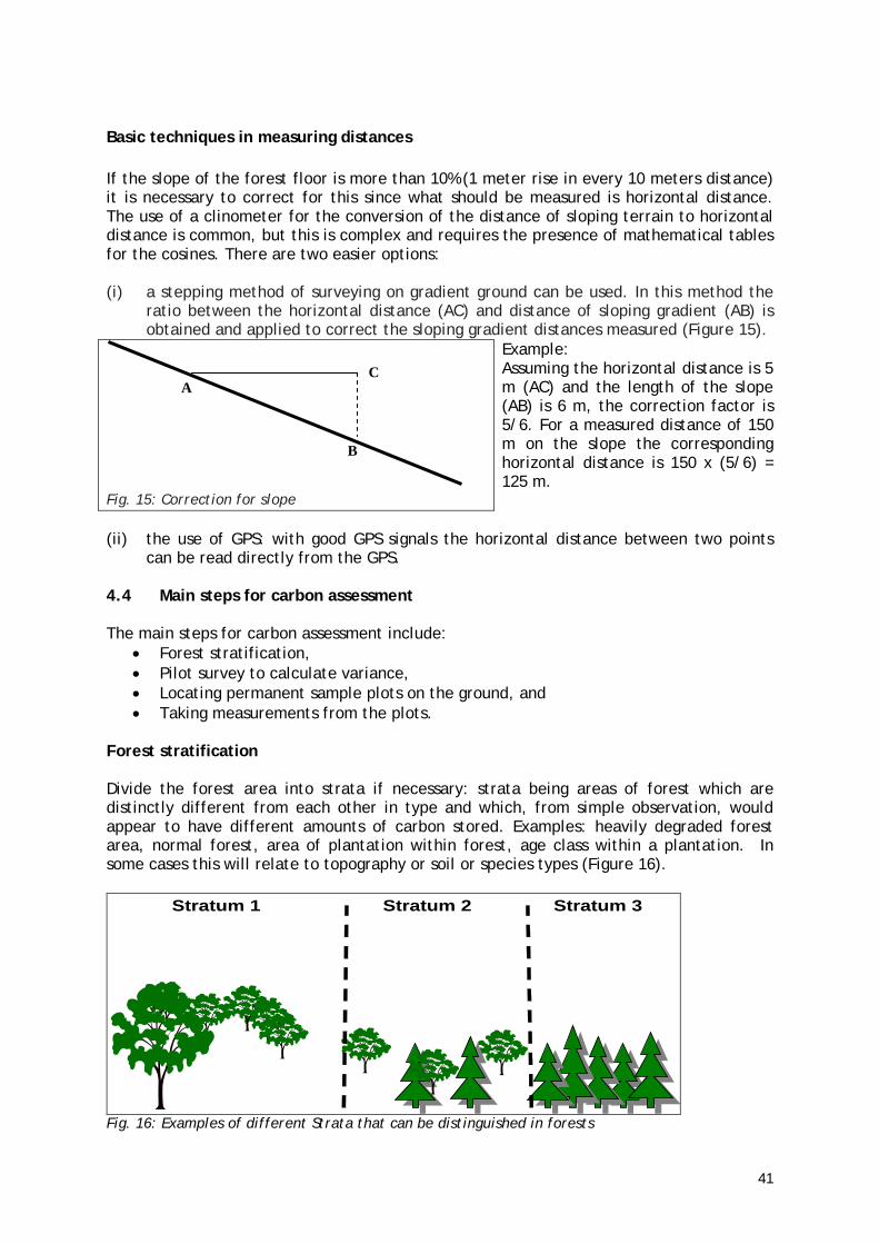
Basic techniques in measuring distances If the slope of the forest floor is more than 10% (1 meter rise in every 10 meters distance) it is necessary to correct for this since what should be measured is horizontal distance. The use of a clinometer for the conversion of the distance of sloping terrain to horizontal distance is common, but this is complex and requires the presence of mathematical tables for the cosines. There are two easier options: (i) a stepping method of surveying on gradient ground can be used. In this method the
ratio between the horizontal distance (AC) and distance of sloping gradient (AB) is obtained and applied to correct the sloping gradient distances measured (Figure 15).
Example: Assuming the horizontal distance is 5 m (AC) and the length of the slope (AB) is 6 m, the correction factor is 5/6. For a measured distance of 150 m on the slope the corresponding horizontal distance is 150 x (5/6) = 125 m.
Fig. 15: Correction for slope (ii) the use of GPS: with good GPS signals the horizontal distance between two points
can be read directly from the GPS. 4.4 Main steps for carbon assessment The main steps for carbon assessment include:
• Forest stratification, • Pilot survey to calculate variance, • Locating permanent sample plots on the ground, and • Taking measurements from the plots.
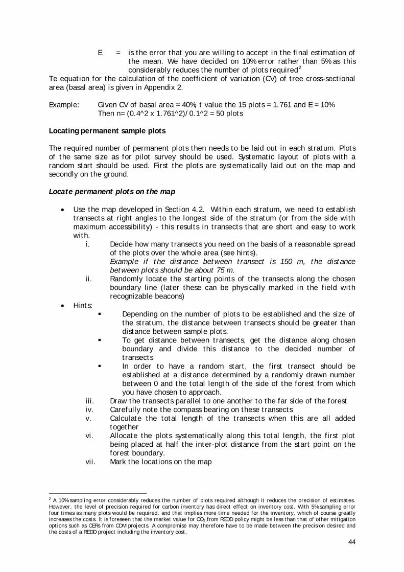
Forest stratification Divide the forest area into strata if necessary: strata being areas of forest which are distinctly different from each other in type and which, from simple observation, would appear to have different amounts of carbon stored. Examples: heavily degraded forest area, normal forest, area of plantation within forest, age class within a plantation. In some cases this will relate to topography or soil or species types (Figure 16). Stratum 1 Stratum 2 Stratum 3
Fig. 16: Examples of different Strata that can be distinguished in forests
A
B
C

42
This exercise should ideally be done jointly between the technical staff and the local community people. As most community forests are characteristically small in size, both boundary tracking and forest stratification is to be done by means of a hand held computer equipped with GPS and ArcPad GIS software. How to establish the forest boundaries has already been explained (section 4.2), and the team should already have carried out this exercise have and become familiar with use of the hand held system. The nature of stratification should first be explained to the community team, who though they may easily think of areas of forest that have very different species present, may not be so quick to see that a degraded patch of forest should be a separate stratum. Discussion on what constitutes ‘different strata’ (in terms of quantity of standing woody biomass, i.e. carbon) should be followed by walking first around the forest boundaries and then if necessary inside the forest area (supporting organization together with the community team) to identify strata (typical tree species and typical condition of trees (stunted, harvested etc). These should then be mapped onto the same basemap as was used for the boundary identification. Typical problems that will be encountered include the fact that the GPS may not work well in dense forest due to difficulties in receiving the signals. With these circumstances, natural land marks such as hills, valley that could be easily identified on a map can be used instead. Pilot survey to calculate variance In each stratum, make a pilot survey to estimate the variance in tree stocking. For this purpose, tree data should be taken from at least 15 sample plots distributed all over each stratum to cover all possible variations. This will allow an estimation of the number of sample plots needed for each stratum based on the observed tree population variation. The plots used for the initial training of community members could be used also for the pilot, to save time and efforts. Steps to be followed:
(i) For estimation of variation of tree stocking at least 15 randomly laid out samples plots distributed to cover all possible variation should be established in each stratum.
(ii) We use nested sample plots (a larger circle containing smaller sub-units) and
measure small trees in small sub-plots and large trees in the whole area (larger circle). This is a strategy to save time as it is expected that, a naturally grown forest has many small size trees and fewer large size trees. The size of the large outer circle of the plot is decided based on the area per tree as described by MacDicken (1997) and presented in Table 1. From Table 1 depending on the density of the trees (column 3) or the nature of vegetation (column 4) you pick your plot size (column 1 and 2). The rule of thumb is that the plot size should accommodate at least 7 large trees.

43
Table 1. Plot radii for carbon inventory plots Plot size (m2)
Plot radius (m)
Area per tree (m2 tree-1)
Nature of vegetation
100 5.64 0 – 15 Very dense vegetation with large number of small diameter stems, uniform distribution of larger stems
250 8.92 15 – 40 Moderately dense woody vegetation 500 12.62 40 – 70 Moderately sparse woody vegetation
666.7 14.56 70 – 100 Sparse woody vegetation 1,000 17.84 > 100 Very sparse woody vegetation
Source: MacDicken (1997)
All trees greater than 10 cm dbh will be measured all over the larger circle. Experience shows that most community managed forests in old degraded forests have many small size trees of < 10 cm dbh and few large trees of > 10 cm Dbh. Therefore, in general sample plots of at least 15m radius will be suitable. For very dense tropical rainy forests such as those in Papua New Guinea and other rainforests, plots with the outer circle of 12.62m, would be large enough to capture sufficient numbers of large trees.
Saplings (i.e. all woody stems longer than 1.3m high but with 1 ≥ dbh≤ 5 cm) will be measured in a small circular plot (of 2m to 5m radius) at the centre of the large circle. A count of regenerating tree species (i.e. very small saplings less than 1cm diameter) will also be made in this subplot.
Data on each tree will be recorded in pre-prepared field forms (Appendix 1)
The size of the sample (number of sample plots needed for any given forest) will depend on a number of factors, but particularly on the variability of the forest (the more variable, the more plots needed in order to get an accurate estimate of overall biomass level). A monoculture of even-aged trees for example will have little variability and require few plot; a mixed natural forest with many different species will have much greater variability. Use of strata (see above) is one of the ways of reducing the effects of variability. The pilot survey provides an initial picture of the variability (the co-efficient of variability or CV), which is then used to calculate how many plots are needed.
The calculation of sample size required is going to be based on the variability of trees and saplings as measured in the pilot survey, so in the pilot survey it is not necessary to sample the herb and grasses layers (although, if the pilot survey is being used as a training exercise, herbs, grasses and soil could also be sampled).
(iii) While walking inside the forest and at a particular plot, try as far as possible to
record tree/shrubs names. These species names will be used to finalize compilation of species checklist to be used for the main inventory.
(iv) With data from the 15 plots, the number of sampling units (n) is calculated
using the formula:
(v) Where: CV = is the coefficient of variation which is the measure of variability of
tree cross-sectional area at breast height t = is the expression of confidence that the true average is within the
estimated range. For 15 plots this always has a value of: 2.32.
2
22
EtCVn =
44
E = is the error that you are willing to accept in the final estimation of the mean. We have decided on 10% error rather than 5% as this considerably reduces the number of plots required2
Te equation for the calculation of the coefficient of variation (CV) of tree cross-sectional area (basal area) is given in Appendix 2.
Example: Given CV of basal area = 40%, t value the 15 plots = 1.761 and E = 10%
Then n= (0.4^2 x 1.761^2)/0.1^2 = 50 plots Locating permanent sample plots The required number of permanent plots then needs to be laid out in each stratum. Plots of the same size as for pilot survey should be used. Systematic layout of plots with a random start should be used. First the plots are systematically laid out on the map and secondly on the ground. Locate permanent plots on the map
• Use the map developed in Section 4.2. Within each stratum, we need to establish transects at right angles to the longest side of the stratum (or from the side with maximum accessibility) - this results in transects that are short and easy to work with.
i. Decide how many transects you need on the basis of a reasonable spread of the plots over the whole area (see hints). Example if the distance between transect is 150 m, the distance between plots should be about 75 m.
ii. Randomly locate the starting points of the transects along the chosen boundary line (later these can be physically marked in the field with recognizable beacons)
• Hints: Depending on the number of plots to be established and the size of
the stratum, the distance between transects should be greater than distance between sample plots.
To get distance between transects, get the distance along chosen boundary and divide this distance to the decided number of transects
In order to have a random start, the first transect should be established at a distance determined by a randomly drawn number between 0 and the total length of the side of the forest from which you have chosen to approach.
iii. Draw the transects parallel to one another to the far side of the forest iv. Carefully note the compass bearing on these transects v. Calculate the total length of the transects when this are all added
together vi. Allocate the plots systematically along this total length, the first plot
being placed at half the inter-plot distance from the start point on the forest boundary.
vii. Mark the locations on the map
2 A 10% sampling error considerably reduces the number of plots required although it reduces the precision of estimates. However, the level of precision required for carbon inventory has direct effect on inventory cost. With 5% sampling error four times as many plots would be required, and that implies more time needed for the inventory, which of course greatly increases the costs. It is foreseen that the market value for CO2 from REDD policy might be less than that of other mitigation options such as CERs from CDM projects. A compromise may therefore have to be made between the precision desired and the costs of a REDD project including the inventory cost.

45
The result of this process is a combined random and systematic sampling frame, with the advantage that the plots can always be found again if the start points along the chosen boundary are known, as well as the bearings and the distances along the transects to each plot.

46
Box 1. Worked example, creating a sampling frame 1. Let us say that the pilot study has indicated that you need 28 sample plots in stratum A and
14 in stratum B. The length of the road as shown in the map (figure 17) is 2.6km. 2. Using a simple calculator pick a random number between 0 and 2.6 (the length of the road)
and mark that point on the road. This is the Starting Point (SP1) for laying out the whole frame for stratum A. It is important that the point is really randomly chosen using some probabilistic method such as those generated by a simple calculator.
3. To spread 28 points our relatively evenly over the area of stratum A you could use 7 transect lines, this means that they will lie exactly 0.4 km (4 cm on the map) from each other.
4. Starting from SP1 measure 0.4 in each direction on the map and mark the starting points of these transects. Draw the transects parallel to one another across the area and note the bearing (70 degrees).
5. Measure the total length of the transect (in our case it is 6.55 km, equivalent to 65.5 cm on the map)
6. Dividing 65.5 by 28 gives a distance of 2.2. In order to space out the plots on the transects, the first plot should be established at half distance i.e. 1.1 cm.
7. Starting with the topmost transect, measure 1.1 cm from its start point and locate the first plot. Since this transect is only 2 cm long, carry the remaining 0.9 cm and add 1.3 m in the next transect and mark the second sample plot, continue from the marking plots at 2.2 cm intervals. (ie operate as if there were one transect of 65.5 cm rather than seven shorter ones)
8. For stratum B, randomly select a Starting Point on the boundary (SP2) and follow the same procedure as was used in stratum A, but for 14 plots only.
It should be noted that the movement explained here is intended for un-experienced surveyor in order grasp the technique. In practice it is more convenient to move directly to the next nearest plot in the next transect if the GPS coordinates of the plot or bearings and distance to it are known. The transect Starting Points can be permanently signaled in the field by use of a beacon or some other permanent marker, such as coloured paint on a central tree in the sample plot. From this the plots can always be found again using compass and measuring tape. GPS recordings can also be made and used.

47
Locate the permanent plots on the ground Actual forest carbon measurement begins when the group meets at the starting point of the first transect. Then a sequence of activities takes place. At first a description of the starting point of a transect and associated landmarks is made and recorded. A foreman in a group then sights the direction using the compass and walks forward along the transect. The other members of the group follow and measure the appropriate inter-plot distance using measuring tape or a stand alone GPS. Upon arriving at the plot centre, mark the plot on the ground by using measuring tape and mark the center with a brightly painted pole. Measure out the circle of selected radius from this point using length of rope. Trees which are on the border are ‘in’ if more than 50% of the basal area falls within the circle and ‘out’ if less than 50%. Overhanging trees are not ‘in’ but trees with trunk in and branches out, are ‘in’. If the slope in the plot is more than 10%, it is necessary to correct for this as detailed in Section 4.2.
(a) Sighting the direction of the transect using a compass,
(b) Measuring distance between plots using a tape measure,
(c) Demarcating a plot using a tape measure (d) Recording details of the description of the plot
to the handheld computer database,
Fig. 18 a-d: Illustrations to show the sequence of activities while locating permanent sample plots on ground

48
Measurements taken from permanent sample plots We are including in the measurements the carbon pools trees/shrubs (above ground biomass only; below ground biomass will be estimated mathematically as a proportion of above ground), litter, dead wood and soil organic carbon. However, not all projects will be looking at all the pools: particularly for the case of soil carbon, it is up to the project team whether they want to include this or not. For the determination of above ground biomass, herbs, grass, litter and soil organic carbon, the following should be done: • Measure the dbh of all trees greater then the minimum dbh within the sample plot
areas and record this information on pre-prepared field forms. Larger trees will be measured over the whole plot and small trees only in the smaller central plot, as described above.
• Set out the quadrats for the shrub and herb layer, cut all vegetation from each
quadrat, weigh it, take a small sample of this in a small bag and label with plot and subplot identification code and record this in pre-prepared forms.
• Collect all litter from the subplot: bag, label, weigh and record. • Take soil samples randomly within the plot; bag and label. Trees The simple way to do this is as we did in the pilot survey, that is to measure all trees over dbh of 1 cm within the small central plot (or 1m radius), and all trees over 5 cm dbh in the whole plot. For this calipers or a diameter tape can be used, start measuring trees clockwise from the direction of transect and from the plot centre, marking each tree as it is done to prevent accidental double counting and recording data on the pre-prepared field forms. A staff of 1.3 m should be used to ensure that readings are taken at exactly the correct height. Each tree is recorded individually with its local name and botanical name. A checklist of the area/forest should be used for consistency in tree naming. It is very important that the same trees are measured every year in each plot (with some recruitment expected). For consistency of measurements in the successive years, the field forms in the database be set up so that measurements in successive years can be compared, as shown in Appendix 1. One possibility is to unobtrusively mark all the trees in each plot so that they can easily be identified every year. Any markings on trees must however be very discrete, because there is a risk that community members deliberately avoid them e.g.: in their normal search for firewood or poles, but instead harvest trees which are not in the sample plot. This would of course bias the sample considerably. From the point of view of carbon storage, it is the large trees, which contribute the most to carbon stock, that are of the most interest, so special care should be taken to make accurate assessments of trees greater than 10 cm dbh. Trees which are already as tall as 1.3m but which are less than 1 cm dbh can hardly be measured, but they can be counted and recorded, and this count will be important especially if comparisons are made from year to year. It could act as an indicator of rate of forest growth (also of sustainability). For what to do with trees of ‘unusual’ shape, please refer to Section 4.2. Most allometric equations and tables are based on dbh and height variables, measuring tree height is therefore important. Usually only a few trees are measured for height in the

49
sample plots and the height of other trees obtained by comparison. In order to get good representative trees it is suggested to take height measure for largest, medium and smallest trees in each plot. The techniques for tree height measurement are described in Section 4.2.
(a) Dbh measurement using tree caliper
(b) Dbh measurement using diameter tape (c) Height measurement using a hypsometer
Fig. 19 a-c: Measuring of tree parameters
Non-tree vegetation, litter and soil Fixed size quadrats or circles (metal, they usually fold up) are used. These are placed on the ground. They are usually one square meter whether round or square. Quadrats do not have to be randomly located within the main plot. However, certain amount of randomization is essential to obviate human bias. Four subplots are recommended to be sampled for each plot as shown in the figure below.
Transect direction
Quadrats
Main plot

50
In the quadrats, sample first for herbs and grasses, then for standing litter and lastly for soil. Include only vegetation that originates within the quadrat, but include and branches that originate within the quadrat and hang over to the outside. Clip all the vegetation down to ground level, place in a sample weighing bag, weigh, and record weight. Take a small sub sample of this vegetation and put in a small bag, label, weigh and take away (has to be dried and reweighed later to account for the moisture content). Collect all biomass litter on the ground, put in a large bag and weigh, record. Take a small sub sample in a small bag, label, weigh and take away for dry weight comparison. Use soil core or slice (first 30 cm of soil), and take one sample from each of the quadrants. Put them all together on a plastic sheet, sieve through a 5mm mesh and mix well. Take a small sample in a bag, label and take away for lab analysis. Record the time Record the time taken, and number of people involved:
• To find and reach the plot • To record all information related to trees • To do the herb and shrub sampling • To do the litter sampling • To do the soil sampling
Including time taken to enter data into the computer

51
5. How to analyze and report the data? From the collected data, forest stand biomass is computed using locally available allometric equations. The most reliable results will be associated with allometric equations which have been locally developed, so it is well worth contacting forest departments or forest colleges to enquire what equations are available and which ones are most used. In absence of local allometric equations, a common procedure is to compute stand volume and convert it to biomass. The volume-biomass conversion factor ranges from 0.5 to 0.6. The biomass is then converted to carbon. The biomass-carbon ratio varies slightly by species and biomass components (trunk, branches etc), but 0.5 (MacDicken, 1997) is recommended if no local value is available. To get the equivalent atmospheric CO2 multiply the carbon by 3.67 since a gram of carbon is about 3.67 grams of CO2. Example: Assuming tree volume per hectare is 68 m3 and the biomass is 42 t/ha, the
carbon is 42 x 0.5 = 21 t/ha. The equivalent CO2 is 21 x 3.67 = 77 tCO2/ha. 5.1 Data analysis for the trees As pointed out above stand biomass is computed from the collected data from plots using available local allometric equations as average sums of trees biomass in the plots. Ideally it is required to check the allometric equations by destructive sampling but if they are used locally, this is not necessary. Also allometric equation may not include branches, twigs and foliage parts of the trees. As such biomass expansion factors should be included to estimate the biomass constituted by these tree parts. Similarly, though below ground estimate of roots biomass represent about 10 to 40% of total tree biomass, it is expensive to determine. It is recommended to include instead an estimate basing on the locally available above ground-roots ratio or equations. The best available literature values relating to a comparable area may be used if local values do not exist. Experience shows that, tropical natural mixed forests are complex ecosystems characterised by high number of different species of different age and sizes. In order to determine; forest stocking (volume, biomass and carbon), tree species composition and structures, and even diversity of these complex forest ecosystems it is logical to express their stand parameters by sizes for each species. Normally this data analysis is done by the use of computer spreadsheets, but this is very cumbersome and liable to errors. For consistence, accuracy and easy of computations, a Tropical Forest Inventory Data Analysis (TROFIDA) package was developed for this purpose (Box 2).

52
5.2 Data analysis for non-tree vegetation, litter and soils Herbaceous, grasses and shrubs can be measured by simple destructive sampling techniques in up to four small subplots per plot as explained above. The samples from each plot are then oven dried to determine dry-to-wet matter ratios. The results are averaged for all the samples taken, giving a per square meter estimate of non-woody biomass. For soil and litter samples required for laboratory analysis, it is recommended to discuss sample needs thoroughly with laboratory technicians before hand to ensure that samples are properly prepared. 5.3 Reporting of carbon data Experience has shown that using appropriate plot sizes, the carbon stocks in natural forest
Box 2. Tropical Forest Inventory Data Analysis (TROFIDA) package TROFIDA consists of computation procedures fitted on Microsoft Access database file to enable computation as fast as data is placed in the database. This database can be used for the computation of important forest stand parameters such as number of stems, basal area, volume, biomass and carbon by species and size classes. The data inputs required are: Tree species checklist Tree species checklist is prepared for each forest by compiling a list of all local names of all different tree species encountered in all the measured plots. This is then followed by matching the local names to their botanical names using locally available tree species checklists (Appendix .. is atypical checklist). The two columns of names are then sorted alphabetically by either local names or botanical names, and assigned species identification codes. Trees data from plots The species identification code for each tree in the sample plot is entered in the data base together with data for dbh and height etc. The data is saved to the computer ready for analysis. Development of height/diameter equation If allometric functions for estimation of trees biomass, volume or carbon require height variable, few trees (sample trees) in each plot are measured for height. Using the sample trees whose heights were measured, a height diameter equation is developed for each forest (vegetation type). Such an equation is used to estimate the height of trees that were measured for dbh only. The Pre-designed Access Database For simplicity of use, the database is designed in such a way that the user need to replace default tree species checklist and trees data tables only. All other computation procedures are already included. The moment when the data for a particular forest are loaded to the database, the forest stand parameters are outright obtained. The stand parameters are separated for each species into diameter classes of convenience. The default diameter classes used in this case are:
dbh class dbh range (cm) 1 <10 2 11-20 3 21-30 4 31-40 5 41-50 6 51-60 7 61-70 8 >70
This database was designed to be used for data analysis by the staff from the local supporting organizations and immediately share the results with the communities. Its applicability that requires the replacement of appropriate allometric equations for the area was tested widely and recommended to be used elsewhere. This database is provided on a separate CD.

53
can be estimated to precision levels within ±10% of the mean, with 90% probability level. The first of these means is that if you carry out measurement in the forest, your average estimate will be within plus or minus 10% of the real value of the carbon stock. The second means that such incidence is likely to happen 90 times out of 100 (i.e. one in ten times, you may be more than 10% above or below the real value). Since carbon credits will be issued on the basis of statistical probability of your estimates being precise, it is important to report these statistics. You can calculate them as follows: 1. Calculate the standard error of the mean from your carbon inventory. This is a
standard operation that can be done on the computer from the data base. 2. Select the confidence level at which you wish to work (we recommend 90%)
CI = X ± tsX
where : X = Mean value of estimate t = is the expression of confidence that the true average is within the estimated
range sX = the standard error of the mean from the carbon inventory
It is also important to show the attained precision levels of estimates (percentage confidence interval to average values of estimates) as shown in Table 1 Table 1: an example for the carbon data reporting
Forest Name KSUATFR
Vegetation type Miombo woodland
Year 2005
Stems ha 694.9±82 (12%)
Volume per ha (m3ha-1) 68.12±16.92 (14%)
Biomass (t ha-1) 42.19±8.65 (9%)
Carbon (t ha-1) 20.39±4.24 (9%)
Mean CO2 t/ha 74.83
Upper limit CO2 t/ha 90.39
Lower limit CO2 t/ha 59.27
The figures in brackets indicate precision levels of estimates i.e. percentage confidence intervals to average value of estimate. It is not certain whether the payment of carbon will be based on average or minimum estimate. It is more likely that minimum estimate will be used that is why it is important to show the average values with their lower and upper limits. The proper inventory planning with stratification is highly important for the generation of high quality i.e. carbon estimates with very high precision.

54

55
6. How to implement? There is no set implementation procedure for this guide. There are of course a few obvious sequences to follow but we advise to let circumstances dictate the course of action. We propose to take the following (general) course of action and adapt it where needed. Some of the points we describe here cannot be handled or decided by your organization alone. These need for instance to be decided by (national) authorities or in conjunction with the communities. Before any project for carbon assessment and monitoring can be done some ground work needs to be done (2 to 3 days, partly in office). The most important issues to cover here are: o Selection of site: in consultation with appropriate authority/ministry at national/
regional level, select potential sites where CFM is working well. o Shortlist local communities that can collaborate in measuring carbon o Visit local communities o Brief orientation on objective and purpose of training o Select communities that agree to be trained o Develop field budget after field locations are identified. o Select at least 8 to 10 people per community to be trained, selection should be done
by the communities themselves. Some level of education is required (at least 5 to 6 years of basic education).
o Select a venue for training Organizing and executing training sessions. For the actual trainings we propose the following schedule which will cover 3 to 5 days depending on the prior knowledge of the participants and the organization of the training. Day 1 (e.g. in village training hall) o Introduction of trainers and trainees
Objective of training Highlight importance of carbon management and its measurement
o Brief introduction to tools, methods and terminology (provide handouts and relevant materials)
o Demo of tools and their application, how to measure a tree, data collection process and how to entry into hard forms and PDA
Day 2 & 3(in the forest) Application of tools and methods in the field. o Stratification of forest and demarcation of forest boundary o Marking points with GPS, setting transects and circular plots, locating centre of plots o Recording dbh, species, etc. into PDA/hard forms o Every trainee must get turns for conducting all activity. o Exercise for data entry at actual field site o Forest Boundary mapping o Data recording for variance estimation and for plot size

56
Day 4 & 5 Session 1 (in village training hall) o Foresters to calculate variance, lay out permanent plots (map) and determine the plot
size. o Plan logistics for forest survey Session 2 (in the forest) o Carry out actually measurement based on sample design
Trainers must assist the trainees and gradually decrease their assistance level with subsequent measurements in different plots.

57
RRReeessseeeaaarrrccchhh ppprrrooojjjeeecccttt “““KKKyyyoootttooo::: TTThhhiiinnnkkk GGGlllooobbbaaalll,,, AAAcccttt LLLooocccaaalll”””
AAA FFFiiieeelllddd GGGuuuiiidddeee fffooorrr AAAsssssseeessssssiiinnnggg aaannnddd MMMooonnniiitttooorrriiinnnggg
RRReeeddduuuccceeeddd FFFooorrreeesssttt DDDeeegggrrraaadddaaatttiiiooonnn aaannnddd CCCaaarrrbbbooonnn SSSeeeqqquuueeessstttrrraaatttiiiooonnn bbbyyy
LLLooocccaaalll CCCooommmmmmuuunnniiitttiiieeesss
PPPaaarrrttt 111::: fffooorrr cccooommmmmmuuunnniiitttiiieeesss PPPaaarrrttt 222::: fffooorrr tttrrraaaiiinnneeerrrsss PPPaaarrrttt 333::: fffooorrr pppooollliiicccyyy mmmaaakkkeeerrrsss
2009

58
This work is licensed under the Creative Commons Attribution-Noncommercial-No Derivative Works 3.0 Netherlands License. To view a copy of this license, visit http://creativecommons.org/licenses/by-nc-nd/3.0/nl/ Project team KYOTO: Think Global, Act Local (K:TGAL) Department of Technology and Sustainable Development University of Twente P.O. Box 217 7500 AE Enschede The Netherlands Telephone: +31 (0)53 489 3545 Fax: +31 (0)53 489 3087 www.communitycarbonforestry.org

59
Table of Contents 1. Introduction ............................................................................. 61 2. The project methodology ............................................................. 63 3. What communities use ................................................................. 65
3.1 Forest Measurements ............................................................. 65 3.2 Mobile GIS .......................................................................... 66
4. Community training. ................................................................... 67
4.1 Selection of the local community trainees and training .................... 67 5. Analysis and reporting ................................................................. 71
5.1 Data analysis ....................................................................... 71 5.2 Reporting of carbon data ........................................................ 71
6. Implementation ...................................................................... 73 7. References ................................................................................. 75

60
61
1. Introduction
Most community forest management in developing countries involves management of natural forests that would otherwise be degraded or deforested and producing carbon emissions. When communities participate in forest management in forests in their vicinity, they generally halt or reduce the rate of deforestation and degradation, and they allow the forest to regenerate, which enhances the forest sink. This type of forest management is not credited under the current carbon payment mechanisms of the Kyoto Protocol (CDM). Under new policy currently (2009) in discussion by the Parties to the UNFCCC, called Reduced Emissions from Deforestation and forest Degradation (REDD), it is possible that community forest management could earn carbon credits. REDD policy would operate on the basis of overall national efforts to slow down loss of carbon from forests. With this mechanism the community managed forests projects could contribute to efforts under the forestry sector to form a country level REDD approach. It is probable that individual projects within the country would then be credited by the country’s government depending on their mitigation levels in the commitment period. This requires that from the start of the project, monitoring is done to determine the standing stock in both the managed project area and unmanaged forests with similar conditions. At any accounting time the difference between the carbon emissions or removals from the without-project activities and the carbon emissions or removals for with-project activities represent the carbon value to be credited. This includes two processes: reduced degradation and forest enhancement i.e. CO2 sequestration. The fundamental requirement for any forestry project to participate in REDD policy is therefore to demonstrate its reduced levels of degradation and increased sequestration. Data for this can, in principle, be obtained through comparing a time series of forest inventories. However, in almost all developing countries, there is no data on forest stock over time because forest inventories have not been carried out systematically. The reason for this is that inventories place heavy demands on forest staff capacity and financial resources. This field guide provides an alternative approach involving local communities in the measurements. Despite the fact that these local people have no formal education in forestry, it is possible to train them to follow the same standard forest inventory protocols as are used by professionals, resulting in data which is as reliable as that produced by professionals. Local people moreover can utilize their indigenous knowledge to collect required forest inventory data, and the inventory can be carried out at low cost compared to one carried out by professional foresters. Since 2003, the Kyoto: Think Global Act Local (K:TGAL) research project has developed and tested procedures and techniques for carbon assessment and monitoring by local communities. The project works with local NGOs and research institutes in Mali, Senegal, Guinea Bissau, Papua New Guinea, Tanzania, Nepal and Uttaranchal (India). The procedures and techniques were tested for different forest types in these countries and this field guide draws experiences from all these countries. Note to the reader This field guide is written in three volumes. Each volume contains similar information but aims towards a different audience. The field guide gives a step-by-step guidance to the procedures and techniques that need to be undertaken at field level. This third part of the field guide is written for people who have a general understanding of forestry and carbon assessment. It is intended for policy makers and interested professionals who wish to understand how the local communities (i.e. a team of community members and staff from a local supporting organization) are

62
trained to implement this methodology of carbon assessment using standard procedures. It is also a guide for policy and decision-makers who need to deal with the community carbon assessment and monitoring output. The guide gives insight into the methodology and community output in relation to national and international carbon policies and treaties. The inventory procedure itself draws heavily on MacDicken (1997), Weyerhaeuser (2000) and on Good Practice Guidance for Land Use, Land-Use Changes and Forestry (Intergovernmental Panel on Climate Change (IPCC), 2003). Elements of these procedures have been adapted and set out in a simple way to meet the needs of non-professional community members. Part one of the field guide is aimed at the local forest communities that should do the actual carbon assessment and monitoring. It explains the methodology and tool operation in a practical and simple way for people with a more limited understanding of English and who have less knowledge and understanding of the tools. The guide aims at people that are already involved in community forest management. Part two of the field guide is aimed at trainers that assist local communities to do their own forest carbon measurement and monitoring. This guide gives all the technical details to perform the carbon assessment with recommended tools. Trainers are most likely from local NGOs or CBOs that have experience with community participation and forestry.

63
2. The project methodology Before an inventory starts, it is in most cases necessary to map the forest. Commonly, communities are allocated sections of forest for management which are delineated on the ground by recognizable land marks, but the site is not officially surveyed. If carbon is to be credited and registered, then an accurate, geo-referenced map is essential. The guide explains how communities can be trained to map boundaries using hand held computers and GPS facilities at very low cost. The same equipment may be used to geo-reference the sample plots so that they may be found again for the subsequent inventories. The carbon stock measurement procedures described in this methodology indicate how carbon can be measured in any given piece of forest. For each individual case, measurements would have to be done for the managed area, and possibly in other nearby unmanaged areas to represent a ‘without project’ case. The same kinds of methods can be used in each. This guide does not give information on how to determine the ‘without project’ baseline area: this would have to be decided in situ according to local conditions. Other, non-carbon GHGs are not included, since estimating these is rather complicated. These emissions are likely to be small in managed forests and in any case less than those in non-managed forest, since in the managed forest there will usually be no burning and no major loss of soil cover, while use of fertilizers is rare. Hence ignoring these additional GHGs will provide a conservative estimate of emissions reductions. The method as given here includes a section on data analysis (i.e. to convert from tree volume to biomass and eventually to carbon weight). In order for this to be applied by local communities (with minimum assistance), a user-friendly database i.e. Tropical Forest Inventory Data Analysis (TROFIDA) package has been prepared (Zahabu and Malimbwi, 2008). TROFIDA incorporates default allometric3
equations; as far as possible these should be replaced with locally developed allometric equations for different countries and locations, since these will give more accurate conversion.
In part one and two an overview of the logic of steps is first given, and then the means of carrying them out is described. In this part these steps are summarized in a similar sequence. It is assumed that prior to implementation of this methodology there is already some background information available on land-use history, maps, landownership and socio-economic situation etc. If forest management has been carried out already by the community under assistance of some outside organization it is possible that such data has been compiled. Monitoring requires provisions for quality assurance and quality control to be implemented in documentation and in procedures. The field guide provides Standard Operating Procedures (SOPs) that should be adhered to all times (with some agreed modifications to suit local conditions). In part two, trainers are made aware that in the field the following should be ensured: the local community team members should be fully cognizant of all procedure and the importance of collecting data as accurately as possible; test plots in the field should be installed as part of training and measure all pertinent components using the SOPs; all field measurements should be checked by qualified person in collaboration with the local communities and any errors followed up (e.g. by checking that
3 Allometry in general is defined as the growth of a part of an organism in relation to the growth of the whole organism or some part of it. Tree allometry narrows the definition to applications involving measurements of the growth or size of trees. Allometric relationships are often estimating difficult tree measurement, such as volume, from an easily-measured attribute such as diameter at breast height (DBH). In forestry allometric equations take on many forms in order to represent relationships between the many various attributes of tree size and growth.

64
the technique used to generate the data was in fact the SOP); a document is filed with the project documents that show that these steps have been followed. We have been experimenting with this field guide in a number of countries with different forest types, and it is proved to be applicable in all these cases. However, according to local conditions (density of forest, nature of the terrain etc), local decisions may have to be made to deviate from what we have suggested here. If adaptations are made, a record should be made of what exactly was done, and why. This record can be submitted to the project database at www.communitycarbonforestry.org for wider dissemination.

65
3. What communities use Many tools exist that can be used by communities to measure and monitor the state of their forest resources. The field guide shows some of the most common tools to use for measurement and also introduces a mobile system to record and possibly report these measurements electronically. This chapter provides a summary of the tools and some technical issues that the users are exposed to in part one and two of this guide. The presented tools are only recommendations of which some have been tested under different conditions and those test results are reflected in this guide. Users are warned to assess if the use of any tool is first of all worth the effort and investment and secondly proper to the situation. Many of the tools described in this guide are relatively expensive and can only be justified if a good return is expected. Most importantly the chosen tools should be practical and useful in the field according to the local situation. Community members that actually do the measurements should be (made) comfortable with the chosen tools. Going for a high-end or most advanced option will not always be the most appropriate. 3.1 Forest Measurements For measuring the most common standing tree variables used in assessing biomass (diameter at breast height and total tree height), ordinary forest survey equipment are recommended (Figure 1). In part one and two it is described in detail how the survey equipment can be used to measure these variables.
A tree caliper for measuring dbh
A tape to measure tree dbh and sample plot size
Hypsometer for tree height measurement
An extendable pole for height measurement
Fig. 1. Tools for tree measurements

66
3.2 Mobile GIS It is often thought that using a computer requires advanced skills that would be beyond those of typical villagers. In fact, most community members who can use a modern mobile telephone will be able to use a GPS (Global Positioning System) or a handheld computer system with GPS after a short training of about one to two days. Thereafter the trainees can put what they have learned into practice, using user manuals in their own language.
Handheld computers (PDAs, see figure 2) with mobile GIS (Geographic Information System) software and a Global Positioning System (GPS) can facilitate forest carbon assessment and monitoring. The mobile GIS provides the user with the ability to bring geo-referenced maps and images into the field with the possibility to add and change the attributes (measured variables) attached to the maps and images during the actual observations. The handheld computer system also provides a useful tool for permanent marking of the sample plots for their later identification. The use of GPS or a Mobile GIS system offers more capabilities than just carbon monitoring. It can also facilitate forest boundary mapping and stratification thus making it wider applicable and a more effective investment. In Appendix 3 a proposed equipment configuration and costs estimation is provided.
The step-by-step guide to the procedures in part one of this guide, allows local communities to be trained on the use of the system and be able to: map their forest reserves rapidly and with precision and, locate permanent sample plots with accuracy.
In part one of this guide practical tips are provided for dealing with common errors and explanations are given how to basically set-up the mobile equipment. The operational steps assume that there is a local technician available to do the advanced set-up of the equipment so users only need to perform operational sequences and steps. When community members however, gain more skills they can use the guide also to set-up the equipment without support as part one and two provide easy pictorials to guide the user through the necessary steps.
Fig. 2: Personal Digital Assistant (PDA)

67
4. Community training. 4.1 Selection of the local community trainees and training The field guide assumes that communities wishing to inventory their forests for the sake of carbon crediting have already been identified and that they are already working with local organizations which foster forest activities and can give some technical support. Contact persons from these organizations together with a team of 4 to 7 villagers participate in the training. Criteria for selection of the community team include education level, knowledge of the forest and gender balance. Training starts with the concepts of forest assessment and monitoring for the generation of scientific data on changing tree stocks of their village forests. The communities are told about the prospects of getting financial income from the carbon benefits of their forests through REDD policy or other mechanisms, but without raising false hopes, since at present there is no mechanism in place for this. Next is training on basic forest mensuration techniques for assessing stock and, if applicable, training on the use of mobile GIS for mapping. The training is designed to enable communities to work in consecutive years without outside support. The methodology is focusing on annual measurements in the managed forests, even though the official reporting interval may be only once in five years. The reason for this is to give greater confidence in the overall values, and to note, and average out, any inter-year variations which may relate to management (or failures of management) or to climate variability. Measurements in managed forest will capture the enhancement (stead state or degradation) in carbon stock as a result of management. If the avoided degradation is to be included, a control forest (i.e. one which is not under management) needs to be inventoried in parallel. Although extensive training and support is only given in the first year, it is considered that support capacity must remain on standby in case of new questions or equipment failure. Basic techniques To train users in the necessary basic techniques the guide provides clear and elaborate pictorials that can be used for instruction and field reference. Figure 3 gives an example of the pictorials used to instruct the measurement of tree diameter at breast height (dbh) for trees with normal and irregular shapes. The guide provides all the possible trees irregularities and similar instructions for measuring total tree heights and setting up a survey plan of the forest.
Fig. 3. Example of pictorials to illustrate measurement techniques for trees dbh
1.3 m
1.3 m 1.3 m
1.3 m
Flat terrain Normal or regular tree Measure dbh at 1.3 m
Sloping terrain Normal or regular tree Measure dbh on the up-
hill side
Flat terrain Measure dbh at 1.3 m from the upper side of
the lean
Forked trees below 1.3 m Consider these as two trees.
Take two separate measurements

68
Main steps for carbon assessment Part one and two of this field guide explain as elaborate as possible the steps that communities need to undertake to assess the carbon in their forests. The main steps for carbon assessment include:
• Forest stratification, • Pilot survey to calculate variance, • Locating permanent sample plots on the ground, and • Taking measurements from the plots.
This exercise should ideally be done jointly between the technical staff and local community people. As most community forests are characteristically small in size, both boundary tracking and forest stratification could be done by means of a hand held computer. When the forest boundaries have already been mapped then the teams are familiar with the use of the handheld system. The nature of stratification is first explained to the community team, who though they may easily think of areas of forest that have very different species present, may not be so quick to see that a degraded patch of forest should be a separate stratum. Supporting organizations, together with the community team identify strata (typical tree species and typical condition of trees, stunted, degraded, harvested etc). These are then mapped onto the same base map as was used for the boundary identification. Pilot survey to calculate variance For each stratum, team members are trained to make a pilot survey to estimate the variance in tree stocking. Data from at least 15 sample plots distributed over each stratum will allow an estimation of the number of sample plots needed for each stratum based on the observed tree population variation. We recommend the use of nested sample plots (a large circle containing smaller sub-units) and measure small trees in small sub-plots and large trees in the whole area (larger circle). This is a strategy to save time as it is expected that, a naturally grown forest has many small trees and fewer large size trees. The size of the large outer circle is decided based on the area per tree as described in the field guide part 2. The size of the sample (number of sample plots needed for any given forest) will depend on a number of factors, but particularly on the variability of the forest (the more variable, the more plots needed in order to get an accurate estimate of overall biomass level). A monoculture forest stand of even-aged trees for example will have little variability and require few plot; a disturbed mixed natural forest with many different species will have much greater variability. Use of strata is one of the ways of reducing the effects of variability. The pilot survey provides an initial picture of the variability (the co-efficient of variability or CV), which is then used to calculate how many plots are needed. The calculation of sample size required is based on the variability of trees and saplings as measured in the pilot survey. In the pilot survey the herb and grass layers are not sampled. The number of sampling units (n) is calculated using the formula:
Where: CV = is the coefficient of variation which is the measure of variability of
tree cross-sectional area at breast height t = is the expression of confidence that the true average is within the
estimated range. For 15 plots this always has a value of: 2.32. E = is the error that you are willing to accept in the final estimation of
the mean.
2
22
EtCVn =

69
We have decided on 10% error rather than 5% as this considerably reduces the number of plots required. A 10% sampling error considerably reduces the number of plots required although it reduces the precision of estimates. However, the level of precision required for carbon inventory has direct effect on inventory cost. With 5% sampling error four times as many plots would be required, and that implies more time needed for the inventory, which of course greatly increases the costs. It is foreseen that the market value for CO2 from REDD policy might be less than that of other mitigation options such as CERs from CDM projects. A compromise may therefore have to be made between the precision desired and the costs of a REDD project including the inventory cost. The equation for the calculation of the coefficient of variation (CV) of tree cross-sectional area (basal area) is given in Appendix 2. Example: Given CV of basal area = 40%, t value for the 15 plots = 1.761 and E = 10%
Then n= (0.42 x 1.7612)/0.12 = 50 plots Locating permanent sample plots The required number of permanent plots is then laid out in each stratum. Plots of the same size as for pilot survey are used. Systematic layout of plots with a random start should be used. First the plots are systematically laid out on the map and secondly on the ground. The result of this process is a combined random and systematic sampling frame, with the advantage that the plots can always be found again if the start points along the chosen boundary are known, as well as the bearings and the distances along the transects to each plot.
(a) Sighting the direction of the transect using a compass,
(b) Measuring distance between plots using a tape measure,
(c) Demarcating a plot using a tape measure (d) Recording details of the description of the plot to
the handheld computer database,
Fig. 4 a-d: Illustrations to show the sequence of activities while locating permanent sample plots on ground

70
Actual forest carbon measurement begins when the group meets at the starting point of the first transect. Then a sequence of activities takes place to locate and record starting points and plot centers (figure 4). Measurements taken from permanent sample plots We are including in the measurements the carbon pools trees/shrubs (above ground biomass only; below ground biomass will be estimated mathematically as a proportion of above ground), litter, dead wood and soil organic carbon. However, not all projects will be looking at all the pools: particularly for the case of soil carbon, it is up to the project team to decide on whether they want to include this or not. Each tree is recorded individually with its local name and botanical name. A checklist of the area/forest should be used for consistency in tree naming. It is very important that the same trees are measured every year in each plot. For consistency of measurements in the successive years, the field forms in the database are set up so that measurements in successive years can be compared, as shown in Appendix 1. From the point of view of carbon storage, it is the large trees, which contribute the most to carbon stock, that are of the most interest, so special care should be taken to make accurate assessments of trees greater than 10 cm dbh. Trees which are already as tall as 1.3 m but which are less than 1 cm dbh can hardly be measured, but they can be counted and recorded, and this count will be important especially if comparisons are made from year to year. It could act as an indicator of rate of forest growth (also of sustainability). Most allometric equations and tables are based on dbh and height variables, measuring tree height is therefore important. Usually only a few trees are measured for height in the sample plots and the height of other trees obtained by comparison. In order to get good representative trees we suggest to take height measurement for largest, medium and smallest trees in each plot.

71
5. Analysis and reporting From the collected data, forest stand biomass is computed using locally available allometric equations. The most reliable results will be associated with allometric equations which have been locally developed, so it is advised to contact forest departments or forest colleges to enquire what equations are available and which ones are most used. In absence of local allometric equations, a common procedure is to compute stand volume and convert it to biomass. The volume-biomass conversion factor ranges from 0.5 to 0.6. The biomass is then converted to carbon. The biomass-carbon ratio varies slightly by species and biomass components (trunk, branches etc), but 0.5 (MacDicken, 1997) is recommended if no local value is available. The equivalent atmospheric CO2 can be obtained by multiplying the carbon by 3.67 since a gram of carbon is about 3.67 grams of CO2. Example: Assuming tree volume per hectare is 68 m3 and the biomass is 42 t/ha, the
carbon is 42 x 0.5 = 21 t/ha. The equivalent CO2 is 21 x 3.67 = 77 tCO2/ha. 5.1 Data analysis As pointed out above stand biomass is computed from the collected data from plots using available local allometric equations as average sums of trees biomass in the plots. Ideally it is required to check the allometric equations by destructive sampling but if the equations are used locally, this is not necessary. Also allometric equations may not include branches, twigs and foliage parts of the trees. In such cases biomass expansion factors are included to estimate the biomass constituted by these tree parts. Similarly, though below ground estimates of root biomass represent about 10 to 40% of total tree biomass, it is expensive to determine this exactly. It is recommended to include instead an estimate basing on the locally available above ground-roots ratio or equations. The best available literature values relating to a comparable area should be used if local values do not exist. Experience shows that, tropical natural mixed forests are complex ecosystems characterised by high number of different species of different age and sizes. In order to determine; forest stocking (volume, biomass and carbon), tree species composition and structures, and even diversity of these complex forest ecosystems it is logical to express their stand parameters by sizes for each species. Normally this data analysis is done by the use of computer spreadsheets, but this is very cumbersome and liable to errors. For consistence, accuracy and easy of computations, a Tropical Forest Inventory Data Analysis (TROFIDA) package was developed for this purpose. Herbaceous, grasses and shrubs are measured by simple destructive sampling. The samples from each plot are then oven dried to determine dry-to-wet matter ratios. The results are averaged for all the samples taken, giving a per square meter estimate of non-woody biomass. For soil and litter samples laboratory analysis is required. It is recommended to discuss sample needs thoroughly with laboratory technicians before hand to ensure that samples are properly prepared. 5.2 Reporting of carbon data Experience has shown that using appropriate plot sizes, within the chosen 90% probability level the carbon stocks in natural forest can be estimated to ±10% of the real value of the

72
carbon stock. Since carbon credits will be issued on the basis of statistical probability of these estimates being precise, importance is given to the way these statistics are reported. Besides the formula to be used we also highlight the importance to show the attained precision levels of the estimates (percentage confidence interval to average values of estimates) and the reporting format as shown in Table 1 Table 1: an example for the carbon data reporting
Forest Name KSUATFR
Vegetation type Miombo woodland
Year 2005
Stems ha 694.9±82 (12%)
Volume per ha (m3ha-1) 68.12±16.92 (14%)
Biomass (t ha-1) 42.19±8.65 (9%)
Carbon (t ha-1) 20.39±4.24 (9%)
Mean CO2 t/ha 74.83
Upper limit CO2 t/ha 90.39
Lower limit CO2 t/ha 59.27
The figures in brackets indicate precision levels of estimates i.e. percentage confidence intervals to average value of estimate. It is not certain whether the payment of carbon will be based on average or minimum estimate. It is more likely that minimum estimate will be used that is why the average values are shown with their lower and upper limits.

73
6. Implementation There is no set implementation procedure for this guide. There are of course a few obvious sequences to follow but we advise to let circumstances dictate the course of action. We propose the user to follow a general course of action and adapt it where needed. Some of the points we describe cannot be handled or decided by users alone. These need for instance to be decided by (national) authorities or in conjunction with the communities. The guide indicates time, resources and chronological order of steps in the general course of action regarding ground work and a basic training For the ground work 2 to 3 days, partly in office, are needed to cover the most important issues like: o Selection of site o Shortlist local communities that can collaborate in measuring carbon o Visit local communities o Brief orientation on objective and purpose of training o Select communities that agree to be trained o Develop field budget after field locations are identified. o Select the people per community to be trained o Select a venue for training For the actual trainings we propose a schedule which will cover 4 to 6 days depending on the prior knowledge of the participants and the organization (study load) of the training. Training will include time indoors but most of the curriculum must be dealt with in the forest. If the actual forest is easily accessible from the training site we advise to use that also for the training as it enables direct establishment of the sample plots. Day 1 indoors training o Introduction of trainers and trainees o Introduction to tools, methods and terminology o Demo of tools and their application Day 2 & 3 in the forest o Application of tools and methods in the field. o Stratification of forest and demarcation of forest boundary o Marking points with GPS, setting transects and circular plots, locating centre of plots o Recording dbh, species, etc. into PDA/hard forms o Data recording for variance estimation and for plot size Day 4 indoors training o Calculating variance, lay out permanent plots (on map) and determine the plot size. o Plan logistics for forest survey Day 5 & 6 in the forest o Carrying out actually measurement based on sample design

74

75
7. References IPCC, 2003. Good Practice Guidance for Land Use, Land-Use Changes and Forestry.
Institute of Global Environmental Strategies, Kanagawa, Japan.
MacDicken, K., 1997. A Guide to Monitoring Carbon Storage in Forestry and Agroforestry Projects, Report No. 1611 N. Winrock International Institute for Agricultural Development, Arlington, USA.
Weyerhaeuser, 2000. International Science Conference on the Role of Boreal Forests and Forestry in the Global Carbon Budget. Edmonton, Alberta, Canada.
Zahabu, E and Malimbwi, R.E., 2008. Participatory Forest Inventory: A Solution to Forest Data Scarcity in Tanzania. Proceeding of the Mpingo Workshop, November 2008, Morogoro, Tanzania.

76
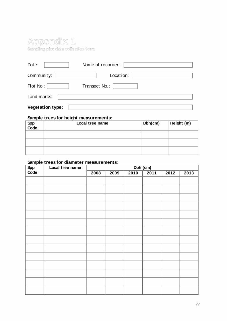
77
Appendix 1 Sampling plot data collection form
Date: Name of recorder: Community: Location: Plot No.: Transect No.: Land marks: Vegetation type: Sample trees for height measurements: Spp Code
Local tree name Dbh(cm) Height (m)
Sample trees for diameter measurements: Spp Code
Local tree name Dbh (cm) 2008 2009 2010 2011 2012 2013

78

79
Appendix 2
The calculation of the coefficient of variation of tree basal area
1. Calculate the mean and the standard deviation of the plot basal areas.
• Basal area of a tree (g) is its cross-sectional area at breast height (1.3m). g = πd2/4
• Plot basal area (Gi m2/ha) is calculated by summing up individual tree basal area in each plot divided by the plot area in hectares. Gi = Σ(g/a)
• Mean plot basal area (G) is then given by G = Σ (Gi/n)
Where d = dbh of the tree in the plot, (cm) g = cross sectional area of tree, m2 a = area in hectares of plot, ha Gi = basal area of plot i, m2/ha G = basal area of plot m2/ha n = number of sample plots
• Standard deviation of plot basal area • CV = Coefficient of variation = standard deviation/mean

80
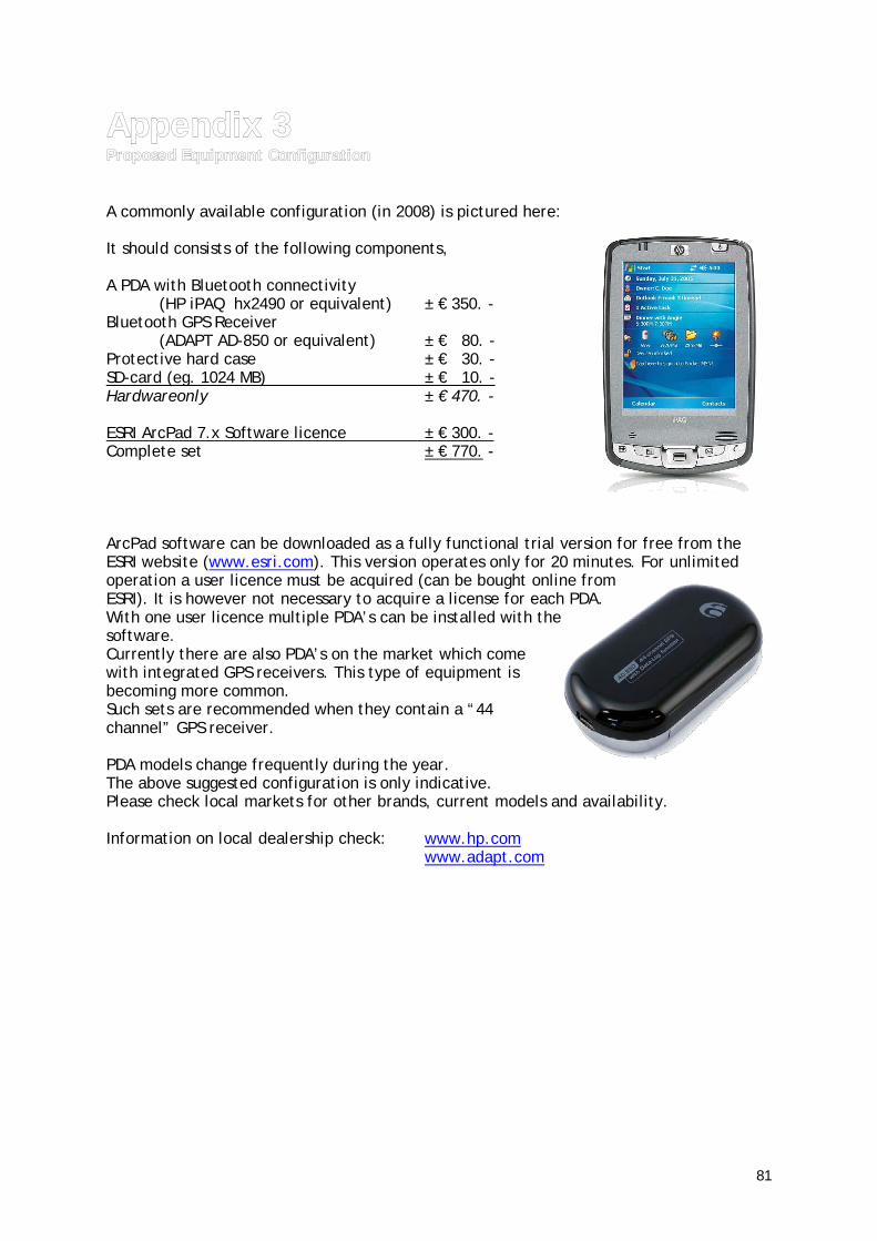
81
Appendix 3 Proposed Equipment Configuration
A commonly available configuration (in 2008) is pictured here: It should consists of the following components, A PDA with Bluetooth connectivity
(HP iPAQ hx2490 or equivalent) ± € 350. - Bluetooth GPS Receiver
(ADAPT AD-850 or equivalent) ± € 80. - Protective hard case ± € 30. - SD-card (eg. 1024 MB) ± € 10. - Hardwareonly ± € 470. - ESRI ArcPad 7.x Software licence ± € 300. - Complete set ± € 770. - ArcPad software can be downloaded as a fully functional trial version for free from the ESRI website (www.esri.com). This version operates only for 20 minutes. For unlimited operation a user licence must be acquired (can be bought online from ESRI). It is however not necessary to acquire a license for each PDA. With one user licence multiple PDA’s can be installed with the software. Currently there are also PDA’s on the market which come with integrated GPS receivers. This type of equipment is becoming more common. Such sets are recommended when they contain a “44 channel” GPS receiver. PDA models change frequently during the year. The above suggested configuration is only indicative. Please check local markets for other brands, current models and availability. Information on local dealership check: www.hp.com www.adapt.com

82
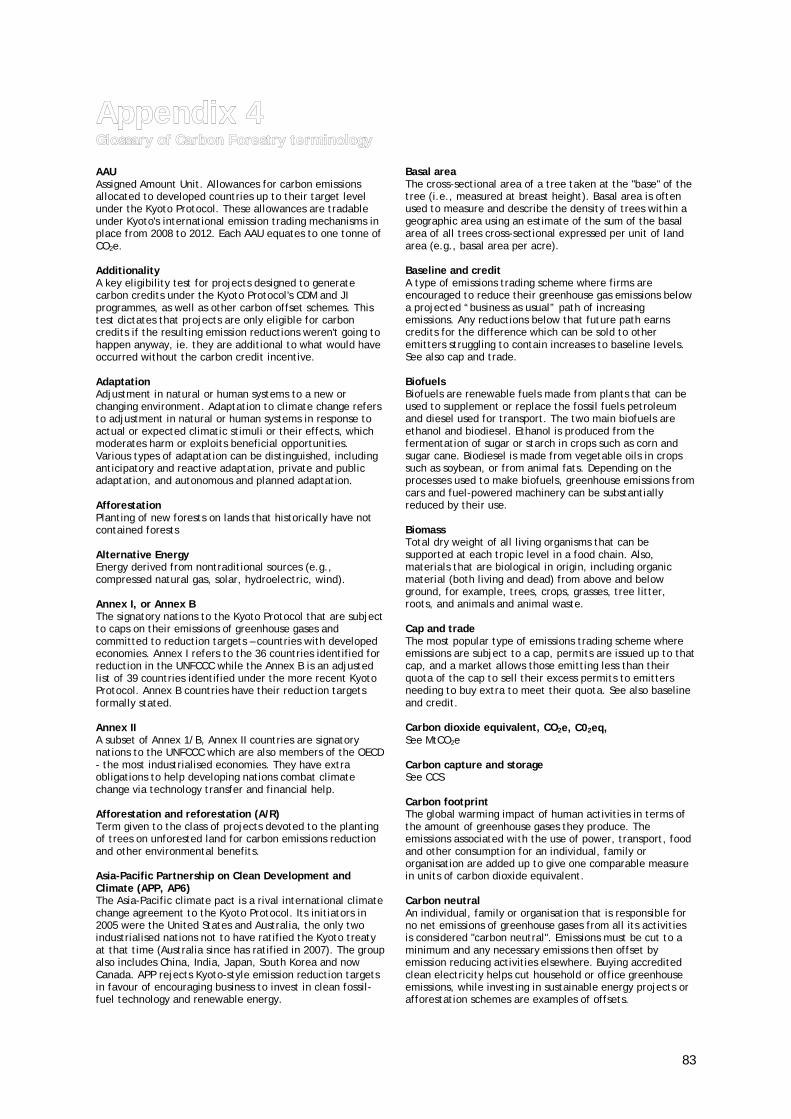
83
Appendix 4 Glossary of Carbon Forestry terminology
AAU Assigned Amount Unit. Allowances for carbon emissions allocated to developed countries up to their target level under the Kyoto Protocol. These allowances are tradable under Kyoto's international emission trading mechanisms in place from 2008 to 2012. Each AAU equates to one tonne of CO2e. Additionality A key eligibility test for projects designed to generate carbon credits under the Kyoto Protocol's CDM and JI programmes, as well as other carbon offset schemes. This test dictates that projects are only eligible for carbon credits if the resulting emission reductions weren't going to happen anyway, ie. they are additional to what would have occurred without the carbon credit incentive. Adaptation Adjustment in natural or human systems to a new or changing environment. Adaptation to climate change refers to adjustment in natural or human systems in response to actual or expected climatic stimuli or their effects, which moderates harm or exploits beneficial opportunities. Various types of adaptation can be distinguished, including anticipatory and reactive adaptation, private and public adaptation, and autonomous and planned adaptation. Afforestation Planting of new forests on lands that historically have not contained forests Alternative Energy Energy derived from nontraditional sources (e.g., compressed natural gas, solar, hydroelectric, wind). Annex I, or Annex B The signatory nations to the Kyoto Protocol that are subject to caps on their emissions of greenhouse gases and committed to reduction targets – countries with developed economies. Annex I refers to the 36 countries identified for reduction in the UNFCCC while the Annex B is an adjusted list of 39 countries identified under the more recent Kyoto Protocol. Annex B countries have their reduction targets formally stated. Annex II A subset of Annex 1/B, Annex II countries are signatory nations to the UNFCCC which are also members of the OECD - the most industrialised economies. They have extra obligations to help developing nations combat climate change via technology transfer and financial help. Afforestation and reforestation (A/R) Term given to the class of projects devoted to the planting of trees on unforested land for carbon emissions reduction and other environmental benefits. Asia-Pacific Partnership on Clean Development and Climate (APP, AP6) The Asia-Pacific climate pact is a rival international climate change agreement to the Kyoto Protocol. Its initiators in 2005 were the United States and Australia, the only two industrialised nations not to have ratified the Kyoto treaty at that time (Australia since has ratified in 2007). The group also includes China, India, Japan, South Korea and now Canada. APP rejects Kyoto-style emission reduction targets in favour of encouraging business to invest in clean fossil-fuel technology and renewable energy.
Basal area The cross-sectional area of a tree taken at the "base" of the tree (i.e., measured at breast height). Basal area is often used to measure and describe the density of trees within a geographic area using an estimate of the sum of the basal area of all trees cross-sectional expressed per unit of land area (e.g., basal area per acre). Baseline and credit A type of emissions trading scheme where firms are encouraged to reduce their greenhouse gas emissions below a projected “business as usual” path of increasing emissions. Any reductions below that future path earns credits for the difference which can be sold to other emitters struggling to contain increases to baseline levels. See also cap and trade. Biofuels Biofuels are renewable fuels made from plants that can be used to supplement or replace the fossil fuels petroleum and diesel used for transport. The two main biofuels are ethanol and biodiesel. Ethanol is produced from the fermentation of sugar or starch in crops such as corn and sugar cane. Biodiesel is made from vegetable oils in crops such as soybean, or from animal fats. Depending on the processes used to make biofuels, greenhouse emissions from cars and fuel-powered machinery can be substantially reduced by their use. Biomass Total dry weight of all living organisms that can be supported at each tropic level in a food chain. Also, materials that are biological in origin, including organic material (both living and dead) from above and below ground, for example, trees, crops, grasses, tree litter, roots, and animals and animal waste. Cap and trade The most popular type of emissions trading scheme where emissions are subject to a cap, permits are issued up to that cap, and a market allows those emitting less than their quota of the cap to sell their excess permits to emitters needing to buy extra to meet their quota. See also baseline and credit. Carbon dioxide equivalent, CO2e, C02eq, See MtCO2e Carbon capture and storage See CCS Carbon footprint The global warming impact of human activities in terms of the amount of greenhouse gases they produce. The emissions associated with the use of power, transport, food and other consumption for an individual, family or organisation are added up to give one comparable measure in units of carbon dioxide equivalent. Carbon neutral An individual, family or organisation that is responsible for no net emissions of greenhouse gases from all its activities is considered "carbon neutral". Emissions must be cut to a minimum and any necessary emissions then offset by emission reducing activities elsewhere. Buying accredited clean electricity helps cut household or office greenhouse emissions, while investing in sustainable energy projects or afforestation schemes are examples of offsets.

84
Carbon price An economic value placed on the emission of greenhouse gases into the atmosphere from human activity. This price is designed to create a disincentive for emissions and incentive to avoid them. A carbon price takes the form of either a carbon tax or an emissions trading scheme. Carbon sink Natural and potentially man-made features on the Earth's surface where carbon dioxide is removed from the atmosphere. The major natural sinks are forests and oceans which have processes that absorb CO2. Carbon sinks are vital to fighting global warming because they counteract sources of carbon emissions, such as industry and transport. Carbon Sequestration The uptake and storage of carbon. Trees and plants, for example, absorb carbon dioxide, release the oxygen and store the carbon. Fossil fuels were at one time biomass and continue to store the carbon until burned. Carbon tax One form of carbon price on greenhouse gas emissions. Set by governments, a price on emissions is fixed and emitters are allowed to emit whatever they want at that price. Emissions trading prices carbon in the reverse approach; fixing emissions, with price varying. CCS Carbon capture and storage. A two-step measure to prevent carbon dioxide being emitted to the atmosphere, particularly from power generation and industrial processes. Instead of venting CO2, it is contained and pumped underground under pressure and sealed off, where it cannot contribute to global warming. This technology is still in its infancy with results largely unproven. CDM Clean Development Mechanism. A Kyoto Protocol initiative under which projects set up in developing countries to reduce greenhouse gas emissions generate tradable credits called CERs, the first step towards a global carbon market. These credits can be used by industrialised nations to offset carbon emissions at home and meet their Kyoto reduction targets. The projects include renewable energy generation, reforestation and clean fuels switching. CER Certified Emission Reduction. A credit generated under Kyoto’s Clean Development Mechanism (CDM) for the reduction of emissions of greenhouse gases equal to one tonne of CO2-equivalent. They are designed to be used by industrialised countries to count toward their Kyoto targets but can also be used by EU companies and governments as offsets against their emissions under the EU Emissions Trading Scheme. See also Offsets. CFI Carbon Financial Instrument. The name of the futures contract through which parcels of emission permits are traded on the European Climate Exchange and the Chicago Climate Exchange. Each CFI consists of 100 permits (mandatory EUAs in Europe and voluntary allowances and offsets on the Chicago market) covering the emission of 100 tonnes of CO2. CO2e Carbon dioxide equivalent. See MtCO2e Cost of carry Generally, the costs associated with holding an investment over time - opportunity costs, fees and other expenses. In carbon markets, where the bulk of trade in emission allowances and credits is in forward contracts for their future delivery, it's largely the time value of money, or the interest rate. Here, 'cost of carry' represents the investment return foregone by the seller (who does not receive the sale
proceeds until delivery) over the contract period, and is reflected in a premium built into forward carbon prices over spot prices. Conference of the Parties (CoP) The supreme body of the United Nations Framework Convention on Climate Change (UNFCCC). It comprises more than 180 nations that have ratified the Convention. Its first session was held in Berlin, Germany, in 1995 and it is expected to continue meeting on a yearly basis. The COP's role is to promote and review the implementation of the Convention. It will periodically review existing commitments in light of the Convention's objective, new scientific findings, and the effectiveness of national climate change programs. Cover Type Expressed as the tree species having the greatest presence (i.e., in terms of volume for older stands or number of trees for younger stands) in a forest stand. Deforestation Those practices or processes that result in the conversion of forested lands for non-forest uses. This is often cited as one of the major causes of the enhanced greenhouse effect for two reasons: 1) the burning or decomposition of the wood releases carbon dioxide; and 2) trees that once removed carbon dioxide from the atmosphere in the process of photosynthesis are no longer present Economies In Transition (EITs) Those nations in Annex I of the Kyoto Protocol considered developed but currently in transition to a market economy. Generally the nations and former republics of the old Soviet bloc. Emissions trading One form of carbon price creating a market-based system for regulating the emission of greenhouse gases. The quantity of emissions is controlled and the price allowed to vary by the issuing of tradable emission permits. These rights to emit can be traded in a commercial market under an emissions trading scheme. ERPA Emissions Reduction Purchase Agreement. Contracts governing the sale of CER carbon credits from UN CDM and JI projects. Heavily used for forward sales of CERs not yet issued, in projects under development, as a means of project financing. The price of such primary CERs is discounted in ERPAs to reflect the risks of non-delivery. ERU Emission Reduction Unit. Tradable credits generated from activities to reduce greenhouse emissions in in industrialised countries, particularly those of the former Soviet-bloc, under the Kyoto Protocol’s Joint Implementation (JI) mechanism. ETS Emissions Trading Scheme. EU ETS European Union Emissions Trading Scheme. EUA European Union Allowances. Tradable emission credits from the EU Emissions Trading Scheme. Each allowance carries the right to emit one tonne of carbon dioxide. Food miles Refers to the distance foodstuffs travel through the various stages of production and processing to the point at which they reach the consumer. A measure of both distance traveled and mode of transportation allows comparisons of the energy use and the contribution to greenhouse

85
emissions associated with various food products and their origin. Forest Stand A group of trees occupying a given area and sufficiently uniform in species composition, age, structure, site quality, and condition so as to be distinguishable from the forest on adjoining areas. Fugitive emissions Unintended leaks of gases into the atmosphere from the extraction, processing or transportation of fossil fuels. For example, gas emissions from leaking pipelines or methane escaping from the ground during the mining of coal. Greenhouse gas (GHG) The three most important greenhouse gases are: o carbon dioxide (CO2), the biggest contributor to global
warming o methane (CH4), eg. from decomposing landfill and
flatulent cattle o nitrous oxide (N20), eg. from vehicle exhaust fumes Greenhouse intensity Refers to the ratio of a nation’s greenhouse gas emissions to its GDP, or the volume of emissions per unit of economic output. A country’s greenhouse intensity may often be falling yet overall emissions are rising due to an expanding economy. Greenhouse intensity measures are also used at a company, plant or industry sector level. Green investment scheme. An arrangement whereby Western industrialised countries buy the surplus Kyoto carbon emissions credits, AAUs, of eastern European countries on the condition they invest the proceeds in low-emissions technology. GISs came about due to pressure on former Soviet bloc countries to use these surpluses, known as "hot air", responsibly, ie. to build environmentally-sustainable industry. GWP Global warming potential. This refers to the potency of greenhouse gases, that is, their ability to trap heat in the atmosphere. The GWP is a numerical measure relative to carbon dioxide, the most abundant greenhouse gas. So carbon dioxide itself has a GWP of 1. For the GWPs of all greenhouse gases. IPCC Intergovernmental Panel on Climate Change. An international scientific panel charged with informing the UNFCCC with the latest scientific evidence on climate change. With representatives from 130 nations it is the world's pre-eminent scientific advisory body on global warming. ITL International Transaction Log. The means by which carbon allowances and credits generated under the mechanisms of the Kyoto Protocol - AAUs, CERs and ERUs - are traded between countries. An online IT platform that connects UN and national greenhouse emissions registries, facilitating the emerging global carbon market. Joint Implementation (JI) A Kyoto Protocol mechanism which allows developed countries, particularly those in transition to a market economy, to host carbon-reducing projects funded by another developed country. The arrangement sees the credits generated, called ERUs, go to the investor country while the emission allowances (AAUs) of the host country are reduced by the same anount. Kyoto Protocol This agreement, which came into force in 2005, commits developed nations collectively to cut their greenhouse gas emissions to 5.2 per cent of 1990 levels by 2012. By 2007,
175 countries had ratified the agreement, including most of the world's developed nations. The Kyoto Protocol was struck in 1997 in Kyoto, Japan, when member nations of the United Nations Framework Convention on Climate Change (UNFCCC) agreed that developed countries must reduce their emissions of six greenhouse gases to meet the overall target, with specific targets varying from country to country. The Protocol came into force in February 2005 and includes 35 developed countries that account for 61.6 per cent of total world carbon dioxide emissions. Leakage, carbon leakage Occurs when laws or activities designed to cut greenhouse gas emissions implemented in one jurisdiction or project area lead to the shifting of the targeted emitting activities elsewhere, thus undermining the attempt to reduce emissions. LULUCF Land use, land use change and forestry. The term given to the sector covering reforestation & afforestation, land clearing and agriculture. Each of these activities can make significant contributions to atmospheric carbon emissions and/or removals. NAPs National Allocation Plans. These set out the overall emissions cap for countries in phases I and II of the EU Emissions Trading Scheme up to 2012, and the emissions allowances that each sector and individual installation within each country receives. Offsets Carbon offsets, offset credits. Credits issued in return for a reduction of atmospheric carbon emissions through projects such as the provision of renewable energy to replace fossil fuel energy, or reforesting cleared land to create a carbon sink. By paying for such emission reducing activities, individuals and organisations can use the resulting credits to offset their own emissions, either voluntarily or under the rules of most emissions trading schemes. One offset credit equates to an emission reduction of one tonne of CO2. See also CER. PDD Project Design Document. The official application drawn up by an entity applying for project approval under the Clean Development Mechanism (CDM). PDDs must be validated by an independent third party, then approved and registered by the CDM Executive Board before a project qualifies as a CER carbon credit earner. REDD Reduced Emissions from Deforestation and Degradation. An initiative to cut greenhouse gas emissions associated with forest clearing by the inclusion of “avoided deforestation” in carbon market mechanisms. More simply, payment in return for the active preservation of existing forests. Reforestation Planting of forests on lands that have previously contained forests but that have been converted to some other use RMUs Removal Units. Credits earned from land use, land-use change and forestry projects (LULUCF) in industrialised countries, including such projects under the Kyoto Protocol’s JI mechanism. Rotation Age The period of years between when a forest stand (i.e., primarily even-aged) is established (i.e., regeneration) and when it receives its final harvest. This time period is an administrative decision based on economics, site condition, growth rates, and other factors.

86
Silviculture The theory and practice of controlling the establishment, composition, growth, and quality of forest stands to achieve certain desired conditions or management objectives. Sink Any process, activity or mechanism which removes a greenhouse gas, an aerosol or a precursor of a greenhouse gas or aerosol from the atmosphere. Soil Carbon A major component of the terrestrial biosphere pool in the carbon cycle. The amount of carbon in the soil is a function of the historical vegetative cover and productivity, which in turn is dependent in part upon climatic variables tCO2e, MtCO2e Tonnes of carbon dioxide equivalent, and millions of tonnes of carbon dioxide equivalent. This is the metric measurement unit for greenhouse emissions. The global warming impact of all greenhouse gases is measured in terms of equivalency to the impact of carbon dioxide (CO2). For example, one million tonnes of emitted methane, a far more potent greenhouse gas than carbon dioxide, is measured as 23 million tonnes of CO2-equivalent, or 23 MtCO2e.
UNFCCC United Nations Framework Convention on Climate Change. Also referred to informally as the UN climate change convention. It is the international agreement for action on climate change and was drawn up in 1992. A framework was agreed for action aimed at stabilising atmospheric concentrations of greenhouse gases. The UNFCCC entered into force on March 1994 and currently has 189 signatory parties. The UNFCCC in turn agreed the Kyoto Protocol in 1997 to implement emission reductions in industrialised countries. VCU Voluntary Carbon Unit. The name of carbon offset credits specifically verified to the Voluntary Carbon Standard, one of the leading independent standards established to demonstrate integrity in project-based emission reductions in the unregulated voluntary carbon market. VERs Verified Emission Reductions. The general name given to carbon offset credits in the voluntary carbon market. These are tradable credits for greenhouse emission reductions generated to meet voluntary demand for carbon credits by organisations and individuals wanting to offset their own emissions.
Sources: www.carbonpositive.net and the online glossaries of IPCC and UNFCCC.

87
Appendix 5 Glossary of Mobile GIS terminology
2D Mode A two-dimensional global positioning system (GPS) position that includes only horizontal coordinates. It requires a minimum of three visible satellites. 3D Mode A three-dimensional GPS position that includes horizontal coordinates plus elevation. It requires a minimum of four visible satellites. .apm file See ArcPad Map file. acquisition time The time it takes for a GPS receiver to acquire a lock onto sufficient satellites—three for 2D mode and four for 3D mode—to calculate a position fix. aerial photograph A photograph of the earth’s surface taken with a camera mounted in an airplane or balloon. Used in cartography to provide geographical information for basemaps. almanac File transmitted from GPS satellites to GPS receivers that contains information about the satellites’ orbits. The receivers use the almanac to decide which satellites to track. altitude 1. The elevation above a reference datum, usually sea level, of any point on the earth’s surface or in the atmosphere. 2. The z-value in a three-dimensional coordinate system. ArcPad Map (.apm) file An ArcPad Map file contains information about the ArcPad Map including the layers in the map, map extent, and settings specific to the map. area 1. Also polygon. A closed, two-dimensional shape defined by its boundary. 2. The size of a geographic feature measured in square units. attribute 1. A piece of information describing a map feature. The attributes of a river, for example, might include its name, length, and average depth. See attribute table. 2. Cartographic information that specifies how features are displayed and labeled on a map; the cartographic attributes of the river in (1) above might include line thickness, line length, color, and font. attribute table A table containing descriptive attributes for a set of geographic features, usually arranged so that each row represents a feature and each column represents one attribute. Each cell in a column stores the value of that column’s attribute for that row’s feature. background image A satellite image or aerial photograph over which vector data is displayed. Although the image can be used to align coordinates, it is not linked to attribute information and is not part of the spatial analysis in a geographic information system (GIS).
bar scale Also scalebar, graphic scale, linear scale. A line used to measure distance on a map, marked like a ruler in units proportional to the map’s scale. bearing (BRG) Also bearing angle. The direction of a fixed point from a point of observation on the earth, expressed as an angle from a known direction, usually north, and usually measured from 0 degrees at the reference direction clockwise through 360 degrees. The terms bearing and azimuth are sometimes interchanged, but in navigation the former usually applies to objects on the earth while the latter applies to the direction of a point on the celestial sphere from a point on the earth. In the ArcPad GPS Position Window, BRG is the compass direction from your current GPS position to the selected destination. column Also field, item. The vertical dimension of a table. Each column stores the values of one type of attribute for all of the records, or rows, in the table. All of the values in a given column are of the same data type (e.g., number, string, blob, date). See attribute table. CompactFlash (CF) Available in Type I or Type II, this is a specific form factor of accessory cards that fit into a respective CF slot. Examples of CF accessory cards include flash memory, mini hard drives, modems, network cards, and GPS receivers. coordinates A set of numbers that designate location in a given reference system such as x,y in a planar coordinate system or x,y,z in a three-dimensional coordinate system. Coordinates represent locations on the earth’s surface relative to other locations. coordinate system 1. A reference system used to measure horizontal and vertical distances on a planimetric map. A coordinate system is usually defined by a map projection; a spheroid of reference; a datum; one or more standard parallels; a central meridian; and possible shifts in the x- and y-directions to locate x,y positions of point, line, and polygon features. 2. In ArcPad, a system with units and characteristics defined by a map projection. A common coordinate system is used to spatially register geographic data for the same area. Course Over Ground (COG) The direction the GPS receiver is moving. COG can be reported in true or magnetic north values. data type The characteristics of columns and variables that define what types of data values they can store. Examples include character, floating point, and integer. datum A set of parameters and control points used to accurately define the three-dimensional shape for the earth—for example, as a spheroid. The datum defines a geographic coordinate system that is the basis for a planar coordinate system. For example, the North American Datum for 1983 (NAD83) is the datum for map projections and coordinates within the United States and throughout North America.

88
decimal degrees (DD) Degrees of latitude and longitude expressed as a decimal rather than in degrees, minutes, and seconds. degree A unit of angular measure represented by the symbol . The circumference of a circle contains 360 degrees. degrees/minutes/seconds (DMS) A measurement of degrees of latitude and longitude in which each degree is divided into 60 minutes, and each minute is divided into 60 seconds. desktop GIS Mapping software that runs on a personal computer and can display, query, update, and analyze geographic locations and the information linked to those locations. Dilution of Precision (DOP) Also Geometric Dilution of Precision (GDOP). An indicator of satellite geometry for a constellation of satellites used to determine a position. Positions with a higher DOP value generally constitute poorer measurement results than those with lower DOP. Factors determining the total GDOP for a set of satellites include, to name a few, Positional DOP (PDOP), Horizontal DOP (HDOP), Vertical DOP (VDOP), and Time DOP (TDOP). directory Also folder. An area of a computer disk that holds a set of data files and/or other directories. Directories are arranged in a tree structure in which each branch is a subdirectory of its parent branch. The location of a directory is specified with a pathname—for example, C:\gisprojects\shrinkinglemurhabitat\grids. display units The units—for example, metric (meters, kilometers), statute (feet, miles), or nautical (knots)—ArcPad uses to report measurements, dimensions of shapes, and navigational speed and distance. distance The amount of space between two things that may or may not be connected, such as two points. Differentiated from length, which always implies a physical connection. See also DST. DST The distance from your current GPS position to the selected destination. DST is displayed in the ArcPad GPS Position Window. See also distance. elevation Also altitude, height. The vertical distance of a point or object above or below a reference surface or datum (generally mean sea level). ephemeris A list of the predicted positions of a GPS satellite for each day of the year or for other regular intervals. Estimated Position Error (EPE) A measurement of horizontal and vertical position error, in feet or meters, based on a variety of factors including DOP and satellite signal quality. feature 1. An object in a landscape or on a map. 2. A shape in a spatial data layer, such as a point, line, or polygon, that represents a geographic object. feature class In a shapefile, coverage, or geodatabase, a collection of spatial data with the same shape type (e.g., point, line, or polygon).
field 1. Also item. A vertical column in a table that represents some characteristic for all of the records in the table, given in numbers or words. 2. The place in a database record, or in a graphical user interface, where data can be entered. file Information stored on disk or tape. A file may be a collection of data, a document (text file), or a program (executable file). It generally resides within a directory and always has a unique name. filename The name that distinguishes a file from all other files in a particular directory. It can refer to the name of the file by itself (harold), the name plus the file extension (harold.shp), or the whole path of a file up to and including the filename extension (C:\mygisdata\shapefiles\harold.shp). filename extension Also file extension. The abbreviation following the final period in a filename that indicates the file’s format—for example, cities.shp, soils.zip, and pigeons.tif. It is usually one to three letters long. geographic coordinates Locations on the surface of the earth expressed in degrees of latitude and longitude. See projected coordinates. georeference To assign coordinates from a known reference system, such as latitude–longitude, Universal Transverse Mercator, or State Plane, to the page coordinates of an image or a planimetric map. global positioning system (GPS) A constellation of 24 satellites, developed by the U.S. Department of Defense, that orbit the earth at an altitude of 20,200 kilometers. These satellites transmit signals that allow a GPS receiver anywhere on earth to calculate its own location. The global positioning system is used in navigation, mapping, surveying, and other applications where precise positioning is necessary. heading The direction of a moving object from a point of observation, expressed as an angle from a known direction, usually north. Bearing and heading differ in that bearing refers to a fixed position, whereas heading refers to the direction in which an object is moving. hyperlink A link that connects a geographic feature to an external image, text, or executable file. When the feature is clicked, the file runs or is displayed onscreen. initialization The first time a GPS receiver orients itself to its current location. After initialization has occurred, the receiver remembers its location and acquires a position more quickly because it does not need to receive a large amount of information from the GPS satellites. label Text placed next to a feature on a map to describe or identify it. latitude The angular distance along a meridian north or south of the equator, usually measured in degrees. Lines of latitude are also called parallels. latitude–longitude Also lat/long, lat/lon. The most commonly used spherical reference system for locating positions on the earth.

89
Latitude and longitude are angles measured from the equator and the prime meridian to locations on the earth’s surface. Latitude measures angles in a north–south direction; longitude measures angles in an east–west direction. layer 1. A set of vector data organized by subject matter, such as roads, rivers, or political boundaries. Vector layers act as digital transparencies that can be laid atop one another for viewing or spatial analysis. 2. A set of raster data representing a particular geographic area, such as an aerial photograph or a remotely sensed image. In both (1) and (2), layers covering the same geographical space are registered to one another by means of a common coordinate system. 3. A file that stores symbology and displays information for a given vector or raster dataset. The layer does not actually contain the data but stores the path to its physical location. line Also linear feature. A shape having length and direction but no area, connecting at least two x,y coordinates. Lines represent geographic features too narrow to be displayed as an area at a given scale, such as contours, street centerlines, or streams, or linear features with no area, such as state and county boundary lines. locale A locale reflects the local conventions and language for a particular geographical region. A given language may be spoken in more than one country; for example, Portuguese is spoken in Brazil as well as in Portugal. Conversely, a country may have more than one official language. For example, Canada has two: English and French. Thus, Canada has two distinct locales: Canadian–English and Canadian–French. Some locale-dependent categories include the formatting of dates and the display format for monetary values. The language determines the text and data formatting conventions, while the country determines the national conventions. Every language has a unique mapping, represented by codepages, which includes characters other than those in the alphabet, such as punctuation marks and numbers. A codepage is a character set and is related to the current locale and language. As such, a locale is a unique combination of language, country, and codepage. location Also position. A point on the earth’s surface or in geographical space described by x,y,z coordinates or by other precise information such as a street address. longitude The angular distance, expressed in degrees, minutes, and seconds, of a point on the earth’s surface east or west of a prime meridian—usually, the Greenwich meridian. All lines of longitude are great circles that intersect the equator and pass through the north and south poles. map 1. A graphical presentation of geographic or spatial information. 2. The document used in ArcPad that lets you display and work with geographic data. A map contains one or more layers of geographic data and various supporting elements such as scalebars. A map has properties, such as scale, projection, and extent. map document In ArcGIS Desktop, the disk-based representation of a map. Map documents can be printed or embedded into other documents. Map documents have an .mxd file extension. map projection A mathematical model that transforms the locations of features on the earth’s curved surface to locations on a
two-dimensional surface. It can be visualized as a transparent globe with a lightbulb at its center casting lines of latitude and longitude onto a sheet of paper. Generally, the paper is either flat and placed tangent to the globe—a planar or azimuthal projection—or formed into a cone or cylinder and placed over the globe—cylindrical and conical projections. Every map projection distorts distance, area, shape, direction, or some combination thereof. map units The units—for example, Metric (meters, kilometers), or Statute (feet, miles)—in which the coordinates of spatial data are stored. menu A command that arranges other commands into a list. multichannel receiver A GPS receiver that tracks several satellites at a time using one channel for each satellite. multipath Also multipath error. Errors caused when a GPS satellite signal reaches the GPS receiver from two or more paths, one directly from the satellite and the others reflected from nearby buildings or other surfaces. Signals from satellites low on the horizon will produce more error; many receivers can mask satellite signals coming from an angle that is too low. NMEA 0183 A standard data communication protocol used by GPS receivers and other types of navigation and marine electronics. offset An offset combines the use of distance, bearing (or angle), and/or inclination (or slope) to determine the location of features. In ArcPad, there are two types of offsets: simple and complex. pan To move an onscreen display window up, down, or sideways over a map or image without changing the viewing scale. path Also pathname. The location of a file or a directory on a disk, given as the drive, directories, subdirectories, and filename, in that order. The path is always specific to the computer operating system. Pocket PC Windows Powered devices running the Windows CE 3 operating system. point Also point feature. A single x,y coordinate that represents a geographic feature such as a telephone pole. polygon A two-dimensional closed feature representing an area such as a state or county. polyline A sequence of points, each pair of which can be connected with a straight line, a circular arc, an elliptical arc, or a Bezier curve. A polyline with a pair of points that is not connected is called a multipart polyline. position Also location. The latitude, longitude, and altitude (x,y,z) of a point, often accompanied by an estimate of error. It may also refer to an object’s orientation—facing east, for example—without referring to its location.

90
project 1. To display a three-dimensional surface, such as the earth, in two dimensions. See projection. 2. In ArcView GIS 3.x, a file that organizes the views, tables, charts, layouts, and scripts used for geographic analysis and mapmaking. A project is similar to a map document in ArcView 8.x. projected coordinate system A reference system that defines the locations of points on a planar surface. projected coordinates A measurement of locations on the earth’s surface expressed in a two-dimensional system that locates features based on their distance from an origin (0,0) along two axes—a horizontal x-axis representing east–west and a vertical y-axis representing north–south. A map projection transforms latitude and longitude to x,y coordinates in a projected coordinate system. See also geographic coordinates. projection file Also PRJ file. A text file that stores the parameters for the map projection and coordinate system of a geographic dataset. raster A spatial data model made of rows and columns of cells. Each cell contains an attribute value and location coordinates; the coordinates are contained in the ordering of the matrix, unlike a vector structure, which stores coordinates explicitly. Groups of cells that share the same value represent geographic features. See also image; compare vector. record A row in a database or in an attribute table that contains all of the attribute values for a single entity. remote sensing Collecting and interpreting information about the environment and the surface of the earth from a distance, primarily by sensing radiation that is naturally emitted or reflected by the earth’s surface or from the atmosphere or by sensing signals transmitted from a satellite and reflected back to it. Examples of remote sensing methods include aerial photography, radar, and satellite imaging. remote sensing imagery Imagery acquired from satellites and aircraft. Examples include panchromatic, infrared black and white, and infrared color photographs and thermal infrared, radar, and microwave imagery. satellite constellation 1. The arrangement in space of a set of GPS satellites. 2. All the satellites visible to a GPS receiver at one time. 3. The set of satellites that a GPS receiver uses to calculate positions. scale The relationship between the dimension of the features on a map and the geographic objects they represent on the earth, commonly expressed as a fraction or a ratio. A map scale of 1/100,000 or 1:100,000 means that one unit of measure on the map equals 100,000 of the same unit on the earth. segment A line that connects vertices. shape The visible form of a geographic object. Most geographic objects can be represented on a map using one of three basic shapes: points, lines, or polygons.
shapefile A vector file format for storing the location, shape, and attributes of geographic features. It is stored in a set of related files and contains one feature class. skyplot The skyplot graphically shows which GPS satellites are visible to the GPS receiver and whether or not they are being used by the GPS to calculate a position. See also satellite constellation. Speed Over Ground (SOG) The actual speed the GPS receiver is moving over the ground. spheroid 1. A three-dimensional shape obtained by rotating an ellipse about its minor axis, resulting in an oblate spheroid, or about its major axis, resulting in a prolate spheroid. 2. When used to represent the earth, a spheroid as defined in (1), but with dimensions that either approximate the earth as a whole or with a part that approximates the corresponding portion of the geoid. symbol A graphic pattern used to represent a geographic feature on a map. Symbols can look like what they represent (trees, railroads, houses), or they can be abstract shapes (points, lines, polygons). Many characteristics define symbols, including color, size, angle, and pattern. symbology The criteria used to determine symbols for features in a layer. A characteristic, or attribute, of a feature may influence the size, color, and shape of the symbol used. table Data arranged horizontally in rows and vertically in columns in a relational database system. A table has a specified number of columns but can have any number of rows. Rows stored in a table are structurally equivalent to records from flat files in that they must not contain repeating fields. toolbar A set of commands, or buttons, that let you carry out related tasks. Universal Time Coordinated (UTC) A universal time standard referencing the time in Greenwich, England. Also referred to as GMT. Universal Transverse Mercator (UTM) A commonly used projected coordinate system that divides the globe into 60 zones, starting at -180 degrees longitude. Each zone extends north–south from 84 degrees north to 80 degrees south, spans 6 degrees of longitude, and has its own central meridian. vector 1. A data structure used to represent linear geographic features. Features are made of ordered lists of x,y coordinates and represented by points, lines, or polygons; points connect to become lines, and lines connect to become polygons. Attributes are associated with each feature—as opposed to a raster data structure, which associates attributes with grid cells. Compare raster. 2. Any quantity that has both magnitude and direction. vertex One of a set of ordered x,y coordinates that constitutes a line or polygon feature. waypoint A GPS term for a permanently stored and named position in the GPS receiver’s memory. In ArcPad, any selected feature is essentially a waypoint, which can be used for GPS navigation.

91
Windows CE A 32-bit operating system from Microsoft, built to run on embedded devices such as Personal Digital Assistants, tablet PCs, and Auto PCs. World Geodetic System of 1984 (WGS84) The most widely used geocentric datum and geographic coordinate system today, designed by the U.S. Department of Defense. GPS measurements are based on wgs84. x,y coordinates A pair of numbers expressing a point’s horizontal and vertical distance along two orthogonal axes, from the origin (0,0) where the axes cross. Usually, the x-coordinate is
measured along the east–west axis, and the y-coordinate is measured along the north–south axis. x,y,z coordinates In a planar coordinate system, three coordinates that locate a point by its distance from an origin (0,0,0) where three orthogonal axes cross. Usually, the x coordinate is measured along the east–west axis, the y coordinate is measured along the north–south axis, and the z coordinate measures height or elevation. zoom To display a larger or smaller region of an on-screen map or image.
Source: Adapted from the ESRI, ArPad 7.0.1 user guide.

92

93
For more information:
www.communitycarbonforestry.org