A Finite Difference Approach to the Valuation of Path Dependent Life Insurance Liabilities*

Bjarke Jensen+ Peter LGchte Jorgensent

Anders Groseng

First version: May 5, 1999 Current version: December 29, 1999

Abstract

This paper sets up a model for the financial valuation of traditional participating life insurance policies. These claims are characterized by their explicit interest rate guarantees and by various embedded option elements, such as bonus and surrender options. Owing to the structure of these contracts, the theory of contingent claims pricing is a particularly well-suited framework for the analysis of their valuation.

The eventual pay-offs from the contracts considered crucially depend on the history of returns on the insurance company’s assets during the contract period. This path- dependence prohibits the derivation of closed-form valuation formulas but we demonstrate that the dimensionality of the problem can be reduced to allow for the development and implementation of a finite difference algorithm for fast and accurate numerical evaluation of the contracts.

*We are grateful for the comments of Yacine Au-Sahalia, Bent Jesper Christensen, and Carsten Sorensen. The usual disclaimer applies. Peter Lochte Jorgensen (the corresponding author) gratefully acknowledges financial support from the Danish Natural and Soctal Science Research Councils. Document typeset m DT&X.

tBRFkredit A/S, Klampenborgvej 20.5, DK-2800 Lyngby, Denmark, Tel. + 45 45 93 45 93, Fax. + 45 45 87 56 49, email: bjj@brf.dk.

iDepartment of Management, University of Aarhus, Bldg. 350, DK-8000 Aarhus C, Denmark, Tel. + 45 89 42 15 44, Fax. + 45 86 13 51 32. ematl: ecolochte@econ.au.dk.

SDepartment of Finance, Aarhus School of Busmess, DK-8210 Aarhus V, Denmark, Tel. + 45 89 48 64 27, Tel. + 45 86 15 19 43, email: gro@hha.dk

279

1 Introduction

Life insurance contracts and pension plans are complex financial securities that come in many

variations. For example, contracts which offer a guaranteed return each year until maturity are

common throughout the EU, the United States, as well as in Japan. The embedded interest rate

guarantee is reminiscent of a financial option, but it is typically not the only option element

that is revealed in a careful study of the details of traditional life insurance products. The

typical contract also entails a more or less specified claim to a fraction of any excess return

(surplus) generated by the investments - i.e. a bonus option. In addition to this, the contracts

are sometimes equipped with a right to terminate the contract prior to maturity. When this

applies the contract is said to contain a surrender option as well.

The presence of one or more option elements in life insurance and pension products presents

a significant challenge to analysts interested in the valuation and optimal management of these

products. However, it is not the options alone that complicate matters. The way in which

returns on assets are calculated, reported, and distributed to policyholders by the issuing

company needs to be carefully considered when evaluating these products. In particular, the

well-established practice of smoothing returns through time’ and that of using book values on

the liability side of the balance sheet induce severe path-dependencies into the contract pay-offs.

Such contract characteristics have not been explicitly considered in previous, related literature.

For example, a large body of literature exists on the valuation of options embedded in unit-

linked (equity-linked) life insurance products (see e.g. Boyle and Schwartz (1977), Brennan and

Schwartz (1976), Brennan and Schwartz (1979), Nielsen and Sandmann (1995) and Grosen

and Jorgensen (1997)). In unit-linked life insurance the contract pay-off is typically linked

directly to the market value of a reference portfolio - the unit - and the embedded guarantee

is almost always a maturity guarantee with some specified absolute amount guaranteed to be

paid at maturity. Defined in this way, unit-linked life insurance contracts can usually be priced

by some adapted version of Black-Scholes option pricing formula (Black and Scholes (1973)).

The situation is fundamentally different when contracts are participating’ (as opposed to

unit-linked) and the embedded options take the form of annual rate of return guarantees and

280

possibly also American-style sell-back (surrender) features. Here matters are considerably

more involved.

The present paper proposes a model in which the above-mentioned contract complexities

are explicitly dealt with, still using the powerful framework of contingent claims analysis as

our valuation tool. The earlier mentioned path-dependencies will be carefully described and

it will become clear that due to their presence, closed formulas for the contract values are

unattainable. In fact, calculating the contract values by the use of numerical methods will also

seem problematic at first glance, but a key observation which reduces the dimensionality of

the problem will prove helpful, and the second core part of the paper explains how a fast and

accurate numerical routine can be applied to the problems at hand.

The outline of the paper is as follows. Section 2 describes the contracts and the dynamic

model in full detail. In section 3, different variants of the contracts are discussed and the gen-

eral valuation approach is introduced. The numerical valuation framework and the associated

finite difference algorithm are described in section 4. Section 5 presents and discusses results

from a wide range of numerical experiments. Finally, section 6 concludes.

2 The Contract and the Dynamic Model

In this section we describe the characteristics of the financial contract which is arranged

between the insurance or pension company and the investor.

A contract of nominal value PO is issued by the company at time zero. The contract is

immediately acquired by an investor for a single premium of Vo. There are no further payments

from or to the contract prior to maturity at time T where the contract is settled by a single

payment from the company to the investor. In general we shall treat PO as exogenously given

whereas V. is to be determined by our model. V. will also be referred to as the fair value of

the contract.

The contract is a contingent claim and we will determine its value process using methods

from the well-developed theory of contingent claims valuation, see for example Duffie (1996).

The pay-off from the contract at the maturity date is denoted P(T) and we shall generally

281

refer to {P(t)} O<t<~ as the account balance process of the contract. _ _

The evolution of P(.) between successive time points in the set T zz { 1,2,. , T} is

determined by the policy interest rate process, {TP(~)}~~T. Specifically, we have

(1) P(t) = (1 + Tp(t)) P(t - l), t E T,

which implies

(2) P(t) = Pa. fi(l + Tp(i)), t E T. El

Time is measured in years, P(.) is updated annually, and the TP(.)S are annualized rates as in

real life contracts. Now, the way in which rp(.) is determined is of course of vital importance.

The modeling of this interest rate crediting mechanism takes the following simplified time t

balance sheet as its point of departure

Exhibit 1

Assets Liabilities

-A(t) P(t)

B(t)

C = A(t) C = A(t)

This balance sheet is not the company balance sheet but rather a snap-shot of the asset and

liability situation in relation to a given contract.

We use the notation A(t) to denote the market value of the asset base backing the contract.

The policy account balance, P(t), which was introduced above, is a book value. Alternatively,

we can think of P(t) as the funds set aside to cover the contract liability - a distributed resewe.

B(t) denotes the undistributed reserve or simply the buffer. Briefly, the point in keeping an

entry such as B(t) is to partly protect the policy reserve, P(t), (and thus in some sense

company solvency) from unfavorable fluctuations in the asset base.

Before we can explain how the policy interest rate is set, we must model the dynamics of

the asset side. For this purpose we specify the following stochastic differential equation

(3) dA(t) = pA(t) dt + gA(t) dW(t), A(0) = Ao.

282

Here, p, 0, and A0 are positive constants and W(t) is a standard Brownian motion defined on

the filtered probability space (C2, 3, P) on the finite time interval [O; T] The asset base thus

evolves through time according to the familiar geometric Brownian motion (GBM).

For the remaining part of the paper it will be convenient to work under the risk-neutral

probability measure, Q, the existence of which is equivalent to the absence of arbitrage op-

portunities, cf. Harrison and Kreps (1979). The distinguishing feature of Q is that under this

measure all prices discounted by the constant risk free rate of interest, r’, will be Q-martingales.

In particular we have

(4) dA(t) = ~/l(t) dt + aA dWQ(t), A(O) = Ao,

where WQ(t) denotes a standard Brownian motion under Q. This stochastic process is the

sole generator of uncertainty in this model.

Turning to the liability side of the balance sheet, the interest rate crediting mechanism is

modeled by specifying the policy interest rate as follows

B(t - 1) ~ - P(t-1) y )> ’

where TG, cy, and y are positive constants to be introduced shortly. Note first that rp(.) is a

discretely updated process and that rp(t) is fixed for the year beginning at time t - 1. This

construction is again motivated by the way in which real life contracts are set up. Further,

it should be realized that (5) is a rule for the dynamic distribution of funds to the investor’s

account. An obvious consequence of (5) is that the investor is always guaranteed a policy

interest rate of at least TC, Hence, TG is the guaranteed interest rate of the contract. Since TG

is assumed to be positive, P(t) will be a strictly increasing process.

As seen from the second term in the max-expression, the interest rate applied to the

investors account balance may, however, exceed TG if the buffer (the undistributed reserve)

is sufficiently large compared to the policy reserve (the distributed reserve). Denoting y as

the target buffer ratio and 0: as the distribution ratio (5) makes sense intuitively: If the

actual/observed buffer relative to the policy account balance exceeds the desired level, y, of

that ratio, the company will attempt to distribute a fraction, cy, of the surplus. To make this

283

perfectly clear, observe that when the buffer is sufficiently large, i.e. when rG < cy

we can write

P(t) = P(t- 1) l,@($+ -7)) (

= qt - 1) + c+qt - 1) - yP(t - 1))

(6) P(t - 1) + +?jt - 1) - B*(t - 1))

where B*(t - 1) = yP(2 - 1) denotes the optimal buffer at time t - 1. From expression

(6) it is immediate that a fixed fraction of the excessive buffer is distributed to the investor’s

account given the condition discussed above.

More generally, by combining (1) and (5) we have the following relation between successive

account balances

(7) =

P(t) = P(t-1) (l+max{rG.cr(H-7)))

P(t-1) A(t - 1) - P(t - 1) _ -,

P(t - 1)

There are a number of important observations to be made from (7). First, note that the

guaranteed interest rate implies a floor under the final payment from the contract of PFTIoo,, E

PO (1 + rG)*. Hence, there is a risk free bond element built into the contract. Second, it

is observed that there is an interest rate option element to the contract. As discussed above

this option element will generally pay off in situations where favorable returns on the assets

have led to a sufficiently large buffer. In the pension and life insurance industry interest in

excess of promised (guaranteed) returns are commonly labeled as ‘bonus’. Hence, we refer to

this option element as the bonus option. 3 Third, it is seen that P(.) is highly dependent on

the path followed by A(t). In other words, there is no easy way of obtaining the probabilistic

distribution of P(T) from recursive substitution of the P(t) s in relation (l), and hence there

is no simple way of establishing the fair present value, V,, of the future pay-off, P(T), and

we must then resort to numerical methods. This will be the subject of the remaining part of

the paper.

284

3 Contract ljpes and Valuation

We will discuss two versions of the contracts introduced above - the European-style and the

American-style contracts, respectively. The European-style contract is defined as the contract

which pays off simply P(T) at the expiration date. From the martingale property of the

discounted value process we can represent the time s value of the contract, VE(s), as

or alternatively as

(9) V”(s) = EQ {e-‘(T-“)P(T)jS,} , v’s E [O,T]

The time s value of the bond element of the contract, D(s), is given as

D(s) = e -r(T-s) . PT FlOO?

(10) = e-‘(T-s) PO (1 + TG)‘,

and the non-negative time s value of the bonus option, I’(s), is therefore residually determined

as

(11) T(s) = P(s) - D(s)

The American-style contract has an extra feature compared to the European type contract in

that it can be terminated at the investor’s discretion at any point in time, 7, prior to time T for

a pay-off of P(T).” This early exercise feature represents an option of separate non-negative

value and it is commonly known as a surrender oprion in the life insurance business.5 In this

case the contract value at time s E [0, T] can be represented as

(12) VA(s) = -ape EQ { e-‘(‘-s)P(7)jC?;,} , s.

where Is,~ denotes the class of S,-stopping times taking values in [sl T]. See e.g. Duffie (1996)

or Karatzas (1988) for details on American option valuation.

If we denote the time s value of the surrender option by O(s) we have

(13) O(s) = VA(s) - D(s) - I-(s),

285

where VA(s), D(s), and r(s) are defined as in (12), (lo), and (11).

Unfortunately, due to the path-dependence of P(.) and our lack of knowledge of the

precise distribution of P(.), the expectations in (9) and (12) cannot be evaluated analytically.

As regards the European-style contract, an obvious possibility is to evaluate the expectation

in (9) by Monte Carlo simulation. This was done in Grosen and Jorgensen (1999) and led to

very accurate results. However, as regards the American-style contract and the valuation of

(12) standard Monte Carlo simulation is no longer a possibility.” Grosen and Jorgensen (1999)

priced the American-style contract by the use of a rather coarse binomial lattice. They analyzed

20-year contracts in a 20-step lattice which presumably is not very accurate.

In the following we establish an alternative unifying valuation framework in which both

contract types can be accurately handled. We shall develop and implement a finite difference

scheme in which the path-dependent variable is conveniently treated as a parameter and in

which the valuation of European vs. American-style contracts is merely a matter of ‘flipping

a switch’ in our algorithm. Note also that whereas the simple Monte Carlo approach used

in Grosen and Jorgensen (1999) requires that the exact solution to the GBM process (3) is

known, the finite difference approach developed below will not be specific to this choice of

process for the evolution in the asset base.

4 The Numerical Valuation Approach

As stated in valuation expressions (9) and (12) at any particular point in time, s, the contract

value is contingent on S,, i.e. the state of the world at time s. However, as a consequence of

the structure of the specific contracts we are studying, all relevant information about the state of

the world at time s will be summarized by the triplet (A(t), P(t). A(s)) where t E TU{O} and

t 5 s < t + 1 < T. This must be true since the process (4) is the sole generator of uncertainty

in this model and since A(t) and P(t) jointly determine the next value of the account balance,

P(t + l), via relation (5). Hence we can substitute the above mentioned triplet with the pair

(A(s), P(t + l)), which is observed at time s (remember that t < s < t + 1). The variable

P(t + 1) can thus be said to summarize relevant information about the path followed by A(.)

286

up to time t and the pair (-4(s), P(t + 1)) is a sufficient statistic for the state of the world at

time s.

The observations above boil down to the fact that we have a two-state-variable problem

on our hands (not counting ‘time’ as a separate state-variable). We can therefore write the

time s value of the path-dependent contingent claim as

(14) v, = V(s, A(s), P(t + l)), t I s < t + 1 < T, t t Y u (0).

At this point we aim at adopting the ‘original’ no arbitrage valuation approach of Black-

Scholes-Merton (Black and Scholes (1973) and Merton (1973)) extended to incorporate an

additional state-variable. We expect that an application of Ito’s lemma to V along with

the familiar hedging argument of Black-Scholes-Merton can establish a partial differential

equation that must be fulfilled by V. A similar idea is exploited for example by Wilmott,

Howison, and Dewynne (1995), who study path-dependent derivative contracts (such as various

types of Asian options) where the second state-variable, say P, is a time integral of the

first state-variable, A. This is an obvious parallel to our situation. Wilmott, Howison, and

Dewynne (1995) show that their valuation functions must satisfy

(15)

where f(A,t) denotes the drift of the P-process. This equation must be solved subject to

contract specific boundary conditions.

A representation of the solution to the valuation problem such as (15) may provide im-

portant insight but there is still a long way to obtaining actual prices. It is unlikely that an

analytical solution to (15) can be established and due to the high dimension of the partial

differential equation, numerical solution will also be a formidable task.

Fortunately the structure of the particular problem studied in this paper allows for con-

siderable simplification. Recall namely that P(.) is updated only discretely and consequently

that it does not change outside the set of time points, r. Between these ‘sampling dates’ the

contract value will change only as a result of changes in time, s, and the state variable, A(s),

and the problematic equation (15) simplifies to the usual Black-Scholes partial differential

287

equatron

(16) g + ;02A2~ + TAG - TV = 0; s EjO, T]\Y.

This is an important observation since numerical solution of a partial differential equation such

as (16) is significantly less involved than numerical solution of the high-dimensional equation

(15). We note that for the European-style claim we have the single terminal condition

(17) r+ = P(T),

whereas for the American-style contract we add the condition

(18) v, 2 P(s), O<s<T,

which reflects the fact that with this kind of contract the account balance is always available

on demand. Note that since the value of P(t + 1) is determined at time t, it will never be

optimal to exercise the contract between two updates of rp(.). Exercising the contract at e.g.

time s, t < s < t + 1, will result in a loss of interest amounting to (eT(S--t) - l)P(t) > 0,

compared to exercising at time t. Hence we only need to check if V, 2 Pt for t in ‘Y U (0).

We move on to consider what happens at the sampling dates t E Y. Along the lines of

Wilmott, Howison, and Dewynne (1995) we first argue that as a consequence of the absence

of arbitrage the contract value cannot change discontinuously across the sampling date. This

is not to say that the function cannot jump for fixed A and P as s varies, but that any joint

realization of (s, A,, PS) will necessarily change V in a continuous manner. The importance

of this argument is that we can connect contract values just before (t-) and just after (t+)

sampling date t by the following continuity condition. We have

v,- = v,+

a V(t-, A(t-),P(t)) = V(t+, A(t+), P(t + 1))

h

(19) V(t, A(t), J’(t)) = V(t, A(t), J’(t + 1))

288

Equation (19) is the continuity or no-jump condition that must be applied at any sampling

date t e ‘T. With this established we can provide the following brief overview of the practical

valuation approach:

1. Start at time T and apply the terminal condition, (17), on a suitable grid in (A, P)-space.

2. For every value of P, solve the Black-Scholes partial differential equation, (16), via a

finite difference scheme applied to the corresponding vector of contract values. This

first step will determine lir-i)+ everywhere in the grid.

3. Apply the no-jump condition to obtain !+/(T-~)- everywhere in the grid.

4. Repeat steps 2 and 3 to obtain Vi- from VC,+~)- everywhere in the grid working back-

wards from t = T - 1 to t = 0.

4.1 Discretization Analysis and the Finite Difference Method

The algorithm described above constitutes merely a rough sketch for a numerical evaluation of

the contracts. As always one must be careful with the detailed implementation of the individual

steps. A number of questions arise, for example, regarding the choice of the mesh size of

the grid in (A, P)-space, which finite difference scheme to use, how to impose boundary

conditions, how to implement the no-jump condition etc. In the following we provide a fairly

detailed description of our implementation of the valuation algorithm outlined above.

As discussed earlier and formalized in (14) the contract value, V, is a function of three

variables, s, A, and P, and we must therefore discretize this value function in three dimensions.

We use as to denote the step length between two updates of V in the time dimension. Similarly,

AA and LIP denote the step size between grid points in the A- and P-dimensions respectively.

289

Since neither A nor P can become negative, the relevant range of the three state-variables

is taken to be

(s.A,P) E 0 = ([O,T] x [o>X] x [O,P]),

where 2 and 7 are large constants such that realizations of the state-variables outside 0 occur

with negligible probability.7 Furthermore, in order to simplify the construction of the grid on

0, in choosing the various parameters, we make sure that I s &, J E &, and K E &

are all positive integers. In this way I is of course the number of equally spaced steps in the

il-direction, J is the number of steps in the P-direction, and K is the number of steps per

year in the time dimension.

Now, since the partial differential equation (16) needs to be solved between any two

successive years, t - 1 and t, t E T, before the no-jump condition is applied cf. earlier, we

introduce the following notation for the value of the contract, V, at a grid point

V$ E V ((t + 1) - I&T, ihA,gLW) ,

wheretE{O ,..., ‘1’-l},O<k~K,O~i~I,andO~~<J.

Having thus introduced the necessary notation we are ready to consider the approximation

of the partial differential equation (16) by some finite difference scheme. The usual first

choice of the financial analyst would be the Crank-Nicolson method, which supposedly has

good convergence properties, see e.g. Duffie (1996). However, our experience with applying

this method to the valuation problem considered in this paper has not been convincing and we

have seen some highly unstable results.

We consequently shifted our attention to the fully implicit method (see e.g. Brennan and

Schwartz (1978), Hull (1997) or Wilmott, Howison, and Dewynne (1995)), with which we ex-

perienced no convergence problems and obtained stable results for even “very dis-continuous”

intermediate conditions, Vc,+ll-. Using the fully implicit method and the notation described

above the discretized version of (16) takes the following form

290

which can be further simplified to the following implicit relation

where

r (i4A) as E” = ~_- CT2 (iAA)2 as 2 AA 2 (AA)“’

H’ = AS

1 + r-as + c2 (~LIA)~ - (3A)2’

r (iLA) as G’=-2ail-

CT’ (dlA)* as 2 (aA)2

In order to solve this finite difference scheme two boundary conditions must be imposed.

These are established as follows. At the boundary A = 0 (i.e. i = 0) equation (16) simplifies

considerably and becomes merely

dV -- dS

7-v = 0.

The corresponding finite difference relation can be written as

(21) V ty+l = (1 - ?-As) v,y.

On the other boundary, i.e. for A = 2 or equivalently i = I, we use the fact that the value of

the contract is approximately linear, i.e.

(22) !f! = 0 for A dA2

---i 0.

Again, rewriting (22) using finite differences yields the relation

(23)

291

Combining now (20), (21) and (23) results in the following convenient matrix representation

of the problem

H’ @ 0 . 0

E2 H2 G2 0

0 E3 H3 G3 . .

: . . . . . . . 0 0 El-2 HI-2 (3-2

0 . . 0 (E’-’ - G’-1) (HI-1 + ‘JG’-1)

vL3 ’ t&+1

V 2-3 t,k+l

VI-“3 t&+1

Note that in order to solve the equation system (24), inversion of the left-hand side matrix

is not required due to its special tri-diagonal form. Instead we can use the special, efficient

procedures which take this &i-diagonal form into account and which are described in e.g. Press

et al. (1989). Note furthermore that once the values Vt$$l, , VtrFiiJ have been calculated

using (24) and once the values VtTi+l and Vtf&l have been obtained by using (21) and (23),

there is no need to keep track of the numbers V$, , V,ft and they can be discarded. This

obviously reduces the computer storage requirements significantly.

We finally consider the implementation of the no-jump condition, (19). To understand how

this can be done, suppose the finite difference method has produced values \;I:,, ‘J&j, which

correspond to the finite computer representation of Vt+ Since the finite computer representation

of V,- corresponds to the values Vtli'l,,, we simply need to code the relationship between Vtz$

and Vt?l,o according to the no-jump condition, (19). This is done in the following way:

292

1. For each i and J in the grid compute

jLlP + max { (jLlP) rG, a ((~LIA - @lP) - (jnP) y)}

Denote the integer part of 3 as j. -

2. If j + 1 < J, compute V,?i,O by using the linear interpolation -

3. If j + 1 > J and hence lies outside the grid then (25) cannot be used. Instead, since for -

large values of P the contract value, V, is approximately linear in P, we can apply the

linear extrapolation

The typical situation where j + 1 5 J is illustrated graphically in Exhibit 2 below. -

Exhibit 2

293

The implementation of the no-jump condition outlined above will perform the transfor-

mation of Vt+ to V,-, and the finite difference scheme can be iterated for another year. This

concludes the discussion of the discretization analysis and the finite difference scheme.

5 Numerical Results and Analysis

In this section we provide - mainly in graphical form - a variety of numerical results from the

implementation of our finite difference algorithm. We choose model parameters from a set

of realistic values and analyze how changes herein affect the value of the contracts and their

implicit elements, i.e. the bond element, the bonus option, and the possible surrender option.

As explained in the previous section, there are also a number of technical constants to

be specified before running the algorithm. We shall not dwell on the considerations made in

this respect but merely note that a large number of experiments have resulted in the values

shown in Table 1 being used globally in the implementations. The finite difference scheme

was coded in Pascal and run on an HP-9000 Unix machine. A complete calculation for a

contract with 20 years to maturity took about 790 seconds on average.

Table 1

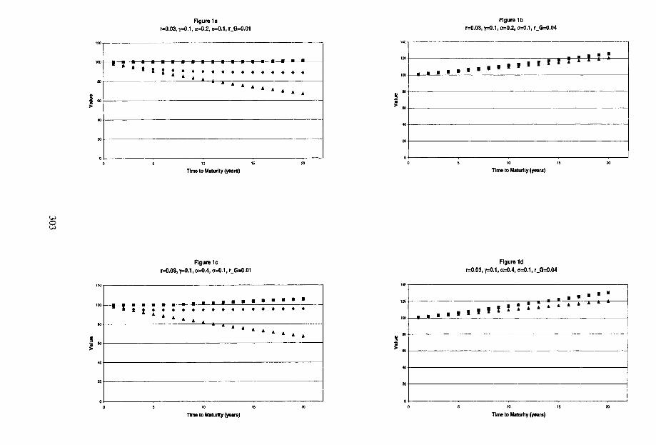
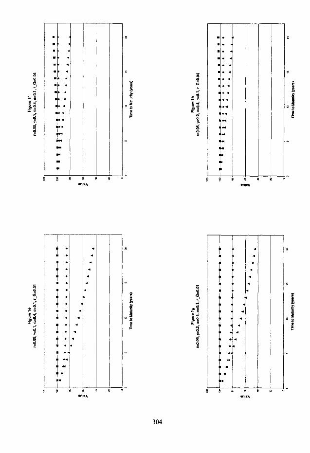
Our numerical results are presented in three different sets of figures (Figures l(a-h), Figures

2(a-d) and Figures 3(a-h)). Throughout the figures we have indexed the initial value of the

asset base and the policy reserve at 100, i.e. A0 = PO = 100.

294

In all figures, a triangle (A) marks the value of the bond element of the contract, a diamond

(4) marks the value of the European contract, and a square (m) marks the value of the American

contract. Generally, the figures confirm that the American type of contract is always at least

as valuable as the otherwise equivalent European contract, which is again more valuable than

the simple bond element implied by the guarantee. Of course, the vertical difference between

a diamond and a triangle in any figure represents the value of the bonus option and similarly,

the vertical difference between a square and a diamond in a figure corresponds to the value of

the surrender option of the contract. The figures are otherwise intended to be self-explanatory

as regards parameters and variables. Below we offer a brief discussion of each of the three

sets of figures:

Figures l(a-h): These figures illustrate the effects of varying the time to maturity, T, of

the contracts. The general picture is that the value of the option elements increases as

the time to maturity increases. More specifically, by comparing Figures la and lc with

Figures lb and Id, the effect of changing the guaranteed interest rate, rG, can be studied.

With the present choice of parameters, the guaranteed interest rate is raised from being

smaller than the market interest rate, T, to being larger than r’. In a sense this means

that the interest rate guarantee has moved from being out-of-the-money to being in-the-

money, and consequently the figures show quite different pictures. Note in particular

that in the case where rG > T (the interest rate guarantee is in-the-money), the surrender

option has virtually no value (i.e. the option to terminate the contract prematurely is

unattractive). Similarly, the bonus option has dropped in value and the contract value

mainly consists of the bond element.

The effect of raising TG can also be studied via a comparison of Figures le and Ig

with Figures If and lh. However, this time rG is not allowed to rise above the market

interest rate. In the more exotic terminology, this means that the interest rate guarantee

remains slightly out-of-the-money and less dramatic effects from the change in TG are

therefore observed. Note again, however, that the values of the option elements decrease

295

with the narrowing of the spread between r and rG. As regards the American type

contracts, Figures le and lg lead us to conclude that the combination of contract terms

and market conditions can be such that the optimal strategy is to exercise the contract

immediately.

Comparing Figures i(a-b) with Figures l(c-d) we see the effect of changing the distri-

bution ratio, cy. As expected, there is a positive relation between cv and the contract

values although the effect of marginal changes in CY is negligible for short maturities.

More interestingly, note that a substitution effect from the surrender option to the bonus

option seemingly exists when a is increased (compare Figures la and lc), but that the

rise in the value of the bonus option more than outweighs the decline in the value of

the surrender option.

If Figures l(e-f) are compared with Figures l(g-h) the effect of raising the target buffer

ratio, y can be studied. For the present choice of parameters the effect is marginal.

However, for large maturities a small decrease in the contract values due to a decline in

the bonus option value is observed. A special situation arises in Figure If where oppo-

site effects in the bonus option and the bond element make the values of the European

contract form a downward hump-shaped curve. The European contract value is thus not

always monotonically increasing/decreasing in the time to maturity.

[See Figures l(a-h) ]

Figures 2(a-d): The effect on contract values of varying the riskless interest rate, r, can be

studied using these figures. The general message is that a larger interest rate implies

larger values of the bonus and surrender options whereas the value of the bond element

declines. It can also be seen that there is always a critical interest rate above which

American contracts should be immediately exercised. This, of course, reflects the fact

that at sufficiently high market interest rates the funds are better invested in riskless

bonds (the interest guarantee is deep out-of-the-money).

296

A direct comparison of Figures 2(a-b) with Figures 2(c-d) shows that raising T-G implies

smaller values of the bonus and surrender options when T is sufficiently large. Further-

more, it is seen that the value of the bonus option is only significant when T is larger

than TG, which reflects the fact that when the interest rate guarantee is in-the-money the

contract values are dominated by the bond element. Conversely, when the guarantee is

out-of-the-money, the option elements become relatively important. This observation is

also confirmed by a direct comparison of Figures la and lc with Figures lb and Id as

described above.

An increase in T yields a larger bonus option value whereas the surrender option remains

largely unaffected for large values of T as can be seen by comparing Figures 2a and 2c

with Figures 2b and 2d.

[See Figures 2(a-d) 1

Figures 3(a-h): In this set of figures the contract values are plotted against the level of

volatility of the assets. It should first be observed that the value of the bond element is

unaffected by this parameter and that the corresponding curves are therefore horizontal.

A second general observation is that the values of both European and American con-

tracts rise with the level of volatility. This is as expected since particularly the bonus

option pays off only when the asset value, ;I,, has been sufficiently high during the

option’s lifetime and since a larger volatility implies a larger probability of high asset

values during the option’s lifetime. This observation is thus in complete accordance

with standard option pricing results and intuition.

Another intriguing observation is that 0 = 0 is not sufficient to make the values of

the option elements equal zero! The reason for this is that when T < rG (and Ba = 0 as

everywhere in the Figures) and cr = 0, the issuing company will clearly never be able

to build reserves for bonus payments and the contracts are in effect above par riskless

297

bonds. Conversely, when rG < r (or even rG < r) and ~7 = 0, the company will surely

be able to build bonus reserves and from some deterministic point in time and onwards

be forced to distribute part of this in the form of bonus. Hence, when T is sufficiently

large, rG < r, and 0 = 0, the value of the bonus option will be strictly positive.

A more specific comparison of Figures 3(a-d) with Figures 3(e-h) reveals the effect

of increasing the riskless interest rate, r. Generally this leads to larger bonus and sur-

render option values.

A comparison of Figures 3(a-b) with Figures 3(c-d) (or Figures 3(e-f) with Figures

3(g-h)) shows the effects of increasing rG. The most striking effect is the decrease in

the value of the surrender option. In fact, the surrender option has effectively vanished

in 3(c-d).

Figures 3a and 3c compared with Figures 3b and 3d (or Figures 3e and 3g compared

with Figures 3f and 3h) show the effects of increasing the time to maturity. As expected,

both the bonus and the surrender option values increase. Note finally how the value of

the bond element also changes in the expected direction as a consequence of the change

in time to maturity.

[See Figures 3(a-h) ]

6 Conclusions

In the present paper we have presented a dynamic model for use in the valuation of the

common family of life insurance products known as participating policies. While the basic

structure of the model was rather simple, it turned out that the attempt to model the interest rate

crediting mechanism in a realistic manner induced a degree of complexity in the model in the

form of path-dependent contract pay-offs which precluded the derivation of explicit valuation

formulas. However, we were able to ‘control’ the path-dependence via the introduction of a

separate state variable, and this observation allowed us to develop a particularly convenient

finite difference scheme for fast and accurate evaluation of the contracts.

It was shown that the typical policy can be decomposed into a riskless bond, a bonus option,

and, if early exercise is allowed, a surrender option. The numerical pricing algorithm developed

was able to calculate the value of each of these contract elements separately. This again allowed

some interesting conclusions to be drawn from the pricing examples in the numerical section

of the paper. Some of the main findings were that values of the participating policies can

be highly sensitive to changes in the time to maturity, changes in the spread between the

guaranteed interest rate and the market interest rate, and to changes in the investment policy

(volatility). In practice, particular attention should be paid to the option elements of these

contracts. They can become quite valuable and can quickly jeopardize the solvency of the

issuer, for example in situations where bonus reserves are low and promised returns are high.

299

Notes

‘See the discussion of the average interest principle in Grosen and Jorgensen (1999).

‘In participating contracts interest is generally credited to the policy account balance ac-

cording to some smoothing surplus distribution mechanism, cf. also later.

3Accordingly, B( .) is often also referred to as the bonus reserve.

4Generally, r can be any date including the off samplin g dates for the American-style

contract. However, it can be shown that the only relevant exercise dates are in fact the

sampling dates, i.e. T E ?” U {0}, cf. also later.

‘For more on surrender options see for example Albizzati and Geman (1994) and Grosen

and Jorgensen (1997).

“There is, however, recent progress in the area of valuing American-style derivatives by

simulation. See e.g. Longstaff and Schwartz (1998).

71n the numerical examples considered in section 5 we have set 3 = 1000 and P = 2000.

300

References

Albizzati, M.-O. and H. Geman (1994): “Interest Rate Risk Management and Valuation of the

Surrender Option in Life Insurance Policies,” Joumul of Risk und Insurance, 61(4):616-637.

Black, F. and M. Scholes (1973): “The Pricing of Options and Corporate Liabilities,” Journal

of Political Economy, 81(3):637654.

Boyle, P. P. and E. S. Schwartz (1977): “Equilibrium Prices of Guarantees under Equity-

Linked Contracts,” Journal of Risk and Insurunce, 44:639-660.

Brennan, M. J. and E. S. Schwartz (1976): “The Pricing of Equity-Linked Life Insurance

Policies with an Asset Value Guarantee,” Journal of Financial Economics, 3:195-213.

(1978): “Finite Difference Methods and Jump Processes Arising in the Pric-

ing of Contingent Claims: A Synthesis,” Journal of Financial and Quantitative Analysis,

13(3):461474.

(1979): “A Continuous Time Approach to the Pricing of Bonds,” Journal of

Banking and Finance, 3: 133-155.

Duffie, D. (1996): Dynamic Asset Pricing Theory, Princeton University Press, Princeton,

New Jersey.

Grosen, A. and P. L. Jorgensen (1997): “Valuation of Early Exercisable Interest Rate Guar-

antees,” Journal of Risk and Insurance, 64(3):481-503.

(1999): “Fair Valuation of Life Insurance Liabilities: The Impact of Interest

Rate Guarantees, Surrender Options, and Bonus Policies,” Working Paper, Department of

Management, University of Aarhus. Forthcoming in Insurance: Mathematics und Economics.

Harrison, M. J. and D. M. Kreps (1979): “Martingales and Arbitrage in Multiperiod Securities

Markets,” Journal of Economic Theory, 20:38 l-408.

Hull, J. C. (1997): Options, Futures, and other Derivatives, Prentice-Hall, Inc., 3rd edition.

301

Karatzas, I. (1988): “On the Pricing of the American Option,” Applied Mathematics und

Optimization, 17:37-60.

Longstaff, F. A. and E. S. Schwartz (1998): “Valuing American Options by Simulation: A

Simple Least-Squares Approach,” Working Paper, The Anderson School at UCLA.

Merton, R. C. (1973): “Theory of Rational Option Pricing,” Bell Journal of Economics and

Management Science, 4:141-183. Reprinted in Merton (1990, Chapter 8).

(1990): Continuous-Time Finance, Basil Blackwell Inc., Padstow, Great Britain.

Nielsen, J. A. and K. Sandmann (1995): “Equity-Linked Life Insurance: A Model with

Stochastic Interest Rates,” Insurance: Mathematics and Economics, 16:225-253.

Press, W. H., B. P. Flannery, S. A. Teukolsky, and W. T. Vetterling (1989): Numerical

Recipes in Pascal, Cambridge University Press.

Wilmott, P., S. Howison, and J. Dewynne (1995): The Mathematics of Financial Derivatives

- A Student Introduction, Cambridge University Press.

302

Flgurela r=O.03,y=O.l, ~0.2, u=O.l, r-G=O.Ol

Figure lc rc0.03,~0.1,oA.4,0=0.1,r~0=0.01

Figure lb r=0.03,yz0.1,as0.2, ~0.1, r-G&04

Flgureld r=O.O3,y=O.1,ci=C~.4, u=O.1,r~G=O.o4

l-7-T-r I : l

! /

/ l :

. .

. .

. . .

. ,, . . II . . I, . .

I :: : : II . . II .

j ,I :. I II

I ‘j-

r-l -a

. .

.

/

9

w

.

.

.

s a a a a o”

304

Flgure2a T~10,y=0.1,a.0.3,0=0.1,LG~0.01

IYI----- __.___ ____--__ _.___._-- ---.-.---- ----7

Figum2c T.1O,yzO.1,a=O.3,o=o.1,r~G=O.O4

Figure2b T=20,y=0.1,a=0.3,0=0.1, r-G=O.Ol

Figure26 T=20,y=O.1,a=0.3,a=O.1, r-G=O.O4

.*, * . . . . l .

. 0 .

. , .

. . .

I . .

. . .

. . .

. l .

I . .

. .

. . .

. . 4

. . .

. , .

. 0 .

. . .

I . .

. . .

. . .

. . .

I . .

I , . .

. .

. .

. .

. .

. .

. .

- I.. . . . . . . 4 . . . . . . . . . . . . . . . . . . . . . . . . .a . .a* . . . . . . . . . . . . . ,. . I. .

. . . . . . . . . . . . . . . . ee w -

! 3 s x

306

I

c P

. 7 . . I . I, . I . . . . . . . I . . . . . . . . . . . I . . . . . . . II .

. . <.

.

.

. * .

5 B a

-4

.

.

.

.

.

.

.

.

.

.

.

.

.

.

.

.

.

.

.

.

.

.

.

.

.

.

.

.

.

+

. . . . . . . . . . . . . . . . . . . . . . . . . . . . .

I a 0

-

I .

. .

I .

. .

. .

. .

I . )

. .

. *

. .

I I .

I , l

. .

. .

. .

. .

. .

.

.

.

. .

.

.

.

.

.

.

.

307

308