JOURNAL OF COMPUTATIONAL PHYSICS 123, 402–414 (1996)ARTICLE NO. 0033

A Finite-Difference Scheme for Three-Dimensional IncompressibleFlows in Cylindrical Coordinates

R. VERZICCO AND P. ORLANDI

Dipartimento di Meccanica e Aeronautica Universita di Roma ‘‘La Sapienza,’’ Via Eudossiana 18, 00184 Rome, Italia

Received January 31, 1995; revised July 6, 1995

that 128 3 128 modes required a memory larger thanthe in-core memory of a CRAY-XMP48. Leonard et al.A finite-difference scheme for the direct simulation of the incom-

pressible time-dependent three-dimensional Navier-Stokes equa- [6] proposed an accurate method for three-dimensionaltions in cylindrical coordinates is presented. The equations in primi- pipe flows with Jacobi polynomials for the radial direction.tive variables (vr , vu , vz and p) are solved by a fractional-step method These polynomials were introduced to minimize thetogether with an approximate-factorization technique. Cylindrical

coupling of the momentum equations, nevertheless thecoordinates are singular at the axis; the introduction of the radialdiscretization produced large nondiagonal sparse matricesflux qr 5 r ? vr on a staggered grid simplifies the treatment of the

region at r 5 0. The method is tested by comparing the evolution to be inverted. Buell et al. [7] developed a Galerkinof a free vortex ring and its collision with a wall with the theory, method to simulate the natural convection in a circularexperiments, and other numerical results. The formation of a tripolar

enclosure. In the radial direction Bessel functions werevortex, where the highest vorticity is at r 5 0, is also considered.used and the condition of finiteness of the solution wasFinally to emphasize the accurate treatment near the axis, the mo-

tion of a Lamb dipole crossing the origin is simulated. Q 1996 Aca- applied at r 5 0. However, the Galerkin method wasdemic Press, Inc. used to reduce the linearized perturbation equations to

an eigenvalue problem and no information was providedabout the extension of the method to the full Navier–

1. INTRODUCTION Stokes equations.A finite volume method was employed by Eggels [8] forIn recent years, thanks largely to direct simulation,

LES in a turbulent pipe. The radial momentum equationgreat advances have been made in the comprehensionrequired an extended gridvolume at the axis to avoid theof transitional and turbulent wall-bounded and free-shearevaluation of quantities at r 5 0. For the same reason,flows. The studies have been limited mainly to planarextrapolations and first-order-accurate differences wereboundaries due to the ease afforded by Cartesian coordi-used at the axis with a reduction of the overall accuracy.nates. Transitional boundary layers [1], turbulent channelNevertheless, in the pipe the decreased accuracy was as-flows [2], and plane mixing layers [3] are examples ofsumed to be not significant due to the smooth behavior ofsuch flows.the flow near the centerline.Many interesting flows, however, require cylindrical co-

Finite-differences are generally less accurate than spec-ordinates even if some of them can be solved in Cartesiantral methods but, on the other hand, they have thecoordinates but to the detriment of accuracy. For example,advantage of being very flexible for complex geometriesMelander et al. [4] performed the simulation of a three-and boundary conditions. Due to this property it hasdimensional round jet in Cartesian coordinates with rea-recently been shown that finite-differences are goodsonable results, but the periodic boundary conditions intro-candidates for direct simulation of complex flows, espe-duced an unphysical perturbation with n 5 4 azimuthalcially when global conservation properties are maintained.wavenumber.Rai et al. [9] and Choi et al. [10] performed this checkIn Cartesian coordinates, within simple boundary con-for the direct simulation of the channel flow, showingditions, very efficient and accurate spectral methods havethat low order statistics are adequately described bybeen developed. The development of an efficient spectralsecond-order schemes while higher accuracies (fourth ormethod in cylindrical coordinates requires a large effortfifth order) are required for high-order statistics. Forto approximate the radial derivatives and to treat thelaminar flows, in particular, second-order accuracy issingularity at r 5 0. Stanaway et al. [5] used spectralsatisfactory (see [11]) and many interesting problemsmethods for axisymmetric flows by introducing special

functions for the radial derivatives. The complexity of requiring cylindrical coordinates, such as round jets [12]and swirling flows can be properly studied. For Cartesianthe scheme is illustrated by the statement of the authors

4020021-9991/96 $18.00Copyright 1996 by Academic Press, Inc.All rights of reproduction in any form reserved.

3D INCOMPRESSIBLE FLOWS 403

coordinates many examples of second-order finite-differ- 2. GOVERNING EQUATIONSence schemes are available in literature; in contrast,

The incompressible Navier–Stokes and continuity equa-presumably due to the singularity at r 5 0 almost notions are rewritten with the quantities qu 5 vu , qr 5 r ? vr ,examples are found for cylindrical coordinates. Schumannand qz 5 vz . In this way the continuity equation assumes[13] developed a finite-difference scheme in cylindrical co-a form similar to that in Cartesian coordinates:ordinates for the simulation of turbulent flows in annuli,

but in that case the flow was confined between two cylin-ders and the singularity at r 5 0 was not encountered. ­qr

­r1

­qu

­u1 r

­qz

­z5 0. (1a)

In this paper a finite-difference scheme for three-dimen-sional incompressible time-dependent flows in cylindricalcoordinates is presented. The scheme, based on a frac- In terms of the qi the momentum equations in conservativetional-step and approximate-factorization technique, is form becomesecond-order accurate in space and time. The major diffi-culty arises from the singularity of the Navier–Stokes equa- Dqu

Dt5 2

1r

­p­u

11

Re F1r S ­

­rr

­qu

­r D2qu

r2 11r2

­2 qu

­u2tions at r 5 0. The introduction of the quantity qr 5 r vr ,on a staggered grid simplifies the discretization of thisregion since qr ; 0 at r 5 0. The scheme is designed to

1­2 qu

­z2 12r3

­qr

­uG,solve wall-bounded as well as free-shear flows with only

minor changes in the procedure, and an example will begiven in Section 5. Dqr

Dt5 2r

­p­r

11

Re Fr­

­r S1r

­qr

­r D11r2

­2 qr

­u2 (1b)The stability and accuracy of the method has been vali-dated by comparing the evolution of an axisymmetric vor-tex ring with that obtained by a vorticity–streamfunction

1­2 qr

­z2 22r

­qu

­uG,

scheme valid for axisymmetric flows. The functional rela-tionship characteristic of the steady translating solutionhas been calculated. When azimuthal perturbations are Dqz

Dt5 2

­p­z

11

Re F1r

­

­r Sr­qz

­r D11r2

­2 qz

­u2 1­2 qz

­z2 G,introduced, these are amplified, at sufficiently high Reyn-olds number, by the self-induced mean strain as describedby Widnall et al. [14]. The numerical results correctly pre- withdicted the most unstable wavenumber (n*) obtained bythe linear stability theory [14], as well as the growth of a Dqu

Dt;

­qu

­t1

1r2

­rquqr

­r1

1r

­q2u

­u1

­quqz

­z,band of modes around n* [15]. The accuracy of the method

was shown by the good agreement between the growth rateof n* and that of the linear theory. To test the feasibility of Dqr

Dt;

­qr

­t1

­

­r Sq2r

r D1­

­uSquqr

r D1­qr qz

­z2 q2

u , (1c)the method to solve flows in presence of walls, we simulatedthe collision of a vortex ring with a wall and the samefeatures as in the experiment of Walker et al. [16] were Dqz

Dt;

­qz

­t1

1r

­qr qz

­r1

1r

­qu qz

­u1

­q2z

­z,

observed. In particular, the trajectories of the centers ofprimary, secondary, and tertiary vortices agreed very well

where in the qu equation the following identities havewith those measured.been used:The vortex ring has a very small amount of vorticity near

the axis; hence, as a severe test of the treatment of the regionaround r 5 0, the case of a tripole formation is considered. 1

r S ­

­rr

­qu

­r D2qu

r2 5­

­r S1r

­rqu

­r D, (1d)This flow has been solved in the r 2 u plane and comparedwith that obtained in Cartesian coordinates [17]. In this flowan accurate discretization near the origin is required since 1

r2

­rqu qr

­r5

1r

­qu qr

­r1

qu qr

r2 . (1e)the peak vorticity is located at r 5 0. A more extreme testof the treatment at the axis is given by the crossing of a Lambdipole through the origin. This flow is not axisymmetric and A characteristic length r0 and a circulation G give the veloc-

ity scale (G/r0) and the pressure scale (r G2/r20 ). The Reyn-with the largest velocities occurring at r 5 0, where there are

also the smallest computational cells. Even if this is one of olds number is Re 5 G/n, with n being the kinematic vis-cosity.the worst applications for polar coordinates, the present

method maintains stability and retains the second-order ac- The advantages of the conservative form for the nonlin-ear terms were emphasized, for two-dimensional flows,curacy for all the velocity components.

404 VERZICCO AND ORLANDI

in the precursor paper by Arakawa [18] for the c 2g (1 2 bl Aiu)(1 2 bl Aiz)(1 2 bl Air) Dqi

formulation, and successively extended to the primitive 5 Dt [cl Hl 1 rl Hl21 2 al Gi pl (3)variables by Grammelwedt [19]. Horiuti [20] also showed 1 al (Aiu 1 Air 1 Aiz) ql

i],that the conservative form minimizes, especially near thewall, the truncation errors associated with central second-

with bl 5 al Dt/2. The solution requires boundary condi-order finite differences. This is a very important require-tions for q and a procedure similar to that suggested inment in wall-bounded flows.[21] yields for the nonsolenoidal field qi 5 q l11

i 1 O(Dt2)The scheme can be applied to flows radially bounded(see Appendix A1).by free-slip or no-slip walls. In the z direction both periodic

The intermediate velocity field q must be globally free-or wall-bounded flows can be considered with only minordivergent, but not locally. The continuity equation is thenchanges in the numerical procedure. Due to the use ofenforced on each cell bytrigonometric expansions in the pressure correction solver

(see Section 3) the method at the moment is limited touniform grids in u and z while a nonuniform grid can be ql11

i 2 qi 5 2al DtGiFl11, (4)

used in the radial direction. This limitation forces the useof a large number of gridpoints in u and z to have a fine

where F is a scalar calculated frommesh instead of allowing clustering only in certain regions.However, the extension to nonuniform grids in all threedirections is now feasible since very efficient multigrid algo-

L Fl11 5 11

al DtD q, (5)rithms to solve elliptic equations in complex regions are

available [10].

In Eq. (5) D and L 5 DG indicate the discrete differen-3. NUMERICAL METHODtial relations

The time-advancement of Eq. (1) employs a fractional-step method extensively described in [21, 9]. However,since by introducing the pressure at the old time step, the D ? 5

1r

d?

du1

1r

d?

dr1

d?

dz, L? 5

1r2

d2?

du2 11r

ddr

rd?

dr1

d2?

dz2 .boundary conditions for the intermediate velocity field qare simplified (N. N. Mansour, personal communication) (6)we wish to shortly summarize the equations to show thesmall differences. The third-order low-storage Runge–

On one side we can note that the dimensions of the termsKutta in combination with the Crank–Nicolson scheme,of D are not the same; however, since it is applied to q (withdescribed in Ref. [9] is used to evaluate the nonsolenoidalqr 5 rvr), the quantity D q has dimensionally correct terms.velocity field q:

We wish to point out that, differently from [9, 21] theintroduction of the pressure pl in Eq. (2) simplifies theqi 2 ql

i

Dt5 Fcl Hl

i 1 rlHl21i 2 alGi pl

(2)boundary conditions for q but, on the other hand, it re-quires the explicit calculation of the pressure gradientsthrough G pl11 5 G pl 1 G Fl11 2 (al Dt/2Re) L G Fl11.

1 al(Aiu 1 Air 1 Aiz)(qi 1 ql

i)2 G. The features of the third-order Runge–Kutta are well

described in [23]; here we only stress that since r1 5 0,each time step is self-starting and a variable Dt can be usedHi contains the convective terms and those viscous termswithout introducing interpolating procedures.with a single velocity derivative, Gi , Aiu , and Aiz denote

discrete differential relations for the pressure and viscousterms, respectively, whose explicit expressions are easily 4. TREATMENT OF THE AXISobtained by straightforward central second-order finite dif-ferences. al , cl , and rl are the coefficients of the time The discretization of the region around r 5 0 is the

most important feature of the present scheme and, in ouradvancement scheme and the same values as [9] have beenused. The implicit treatment of the viscous terms of Eq. opinion, the difficulties in its accurate representation are

the reason for the few simulations in literature. It might(2) would require for the solution the inversion of largesparse matrices, these are reduced to three tridiagonal seem that in Eqs. (1) there are lots of singularities, how-

ever, the most are only apparent. In fact the advantage ofmatrices by a factorization procedure with error O(D t3)[22]. By using the increment Dqi 5 qi 2 q l

i Eq. (2) can be using a staggered grid is that only the component qr isevaluated at the grid point j 5 1 (r 5 0), and there qr 5written in delta form, giving

3D INCOMPRESSIBLE FLOWS 405

5 21

(r3/2)2 F(qu)5/2 1 (qu)3/2

2Drr2G (8a)

11

r3/2F(r qu)5/2 2 (r qu)3/2

Dr2

(r qu)3/2 2Dr G 1

Dr.

The evaluation of (drqu/dr)uj51 by a forward first-order accu-rate expression reduces the overall accuracy of the scheme.The reduced accuracy is not relevant in flows with negligi-ble qu at the axis (vortex rings) but it is important whenqu is present, even when it has a smooth profile.

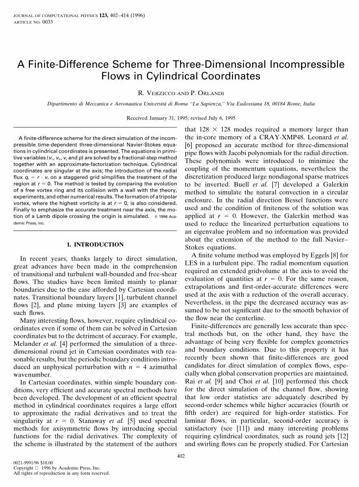
The second expression is

FIG. 1. Sketch of the computational cells: (a) cell at the axis; (b) cellin the domain. 1

rddr

rdqu

dr2

qu

r2 Uj53/2 (8b)

0 by definition (Fig. 1). The equation for qr can be then5

1r3/2

Fr2(qu)5/2 2 (qu)3/2

Dr G 1Dr

2(qu)3/2

(r3/2)2 .discretized for all j $ 2 straightforwardly. A further advan-tage of using a staggered grid is that when qu is not zeroat r 5 0 (see, for example, Section 5.4), it switches signs

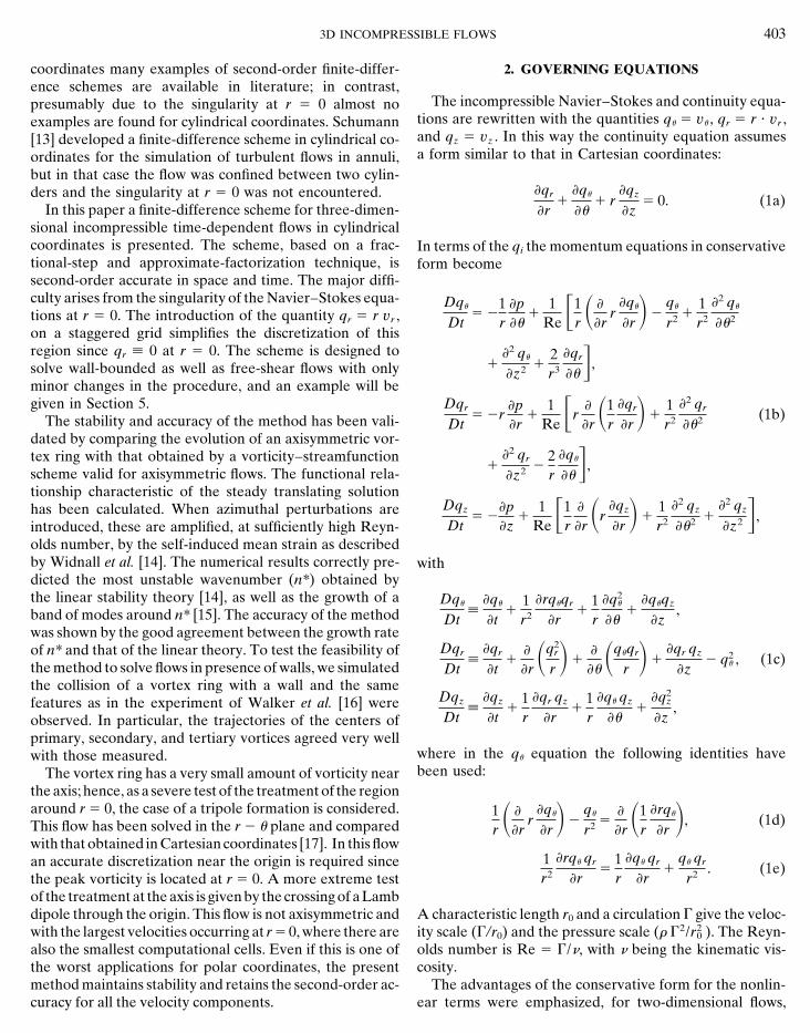
Since in this case r1 ; 0 no approximations have beenat the origin; however, this singularity is automatically han-done and the derivative maintains its second-order accu-dled by this grid since the qu-equation is evolved onlyracy at the axis.1 As a check for Eq. (8a) and Eq. (8b) westarting from the radial location j 5 Ds.considered the axisymmetric vorticity distribution of anThe equations for qz and qu at j 5 Ds require the evaluationisolated monopole, given in [17], whose instability leadsof radial derivatives in the region around r 5 0. The factto the tripole formation (see Section 5.3)that qr ; 0 at j 5 1 avoids the evaluation of qu and qz at

j 5 1 and the radial derivatives of the convective termscan be discretized without any approximation.

gz(r) 5 F1 212

a S r%DaG e2(r/%)a

, (9)On the other hand, the viscous radial derivative for qz

is (only the radial indices are indicated):

where a controls the steepness of the vorticity gradientsand % controls the size of the monopole. From the defini-1

rddr

rdqz

dr Uj53/2

51

r3/2Fr2

(qz)5/2 2 (qz)3/2

Dr2 G, (7)tion of gz at the axis (gz 5 (1/r)(­rqu/­r)) the viscousradial derivative for qu has been analytically computed andthe results compared with those obtained by Eqs. (8a) andand the opportunity to have r1 ; 0 avoids the approxima-(8b). For r @ 0 both expressions give identical results; ontion of dqz/druj51 with a reduced accuracy. However, in thethe contrary at r 5 0 and in its neighbor large differencescase of flows within annuli it results that r1 5/ 0 and the

radial derivative is discretized by first-order approxima-tions as usually done in Cartesian coordinates [9].

1 A third possible expression isThe viscous derivative for qu can be written in two ways.The form on the right-hand side of Eq. (1d), usually foundin textbooks, can be discretized only when it is expanded as 1

r2

ddr

r3 ddr

qu

r Uj53/2

51

(r3/2)2 F(r2)3(qu /r)5/2 2 (qu /r)3/2

Dr G 1Dr

. (8c)

In this case the only assumption is r3 (d/dr)(qu /r) u j51 5 0 and this is not­

­r1r

­rqu

­r5 2

1r2

­rqu

­r1

1r

­2 rqu

­r2 ,true if (d/dr)(qu /r) u j51 R y as r23. However, it is not difficult to showthat r3 ­uu /­r vanishes at the axis for a Cy velocity field. This is becauseas r R 0, uu p rimi21 for the mth azimuthal Fourier mode provided m 5/giving the discretized form0 while for m 5 0 we have uu p r. This expression seems to be accurateas expression (8b) (see Fig. 2), and, in fact, for all cases simulated in the(r 2 x)-plane the same results have been obtained. For nonaxisymmetric

21r2

drqu

dr1

1r

d2 rqu

dr2 Uj53/2

cases, however, like that in Section 5.4 the expression (8b) gives the mostaccurate results and has to be used for full three-dimensional simulations.

406 VERZICCO AND ORLANDI

further changes in the Navier–Stokes equations withoutleading to any improvement of the results.

5. NUMERICAL RESULTS

In this section we present some applications of thescheme to different flows. Comparison with theoretical,experimental, and numerical results obtained by differentmethods are also shown to prove the qualities of themethod.

5.1. Free Vortex Ring

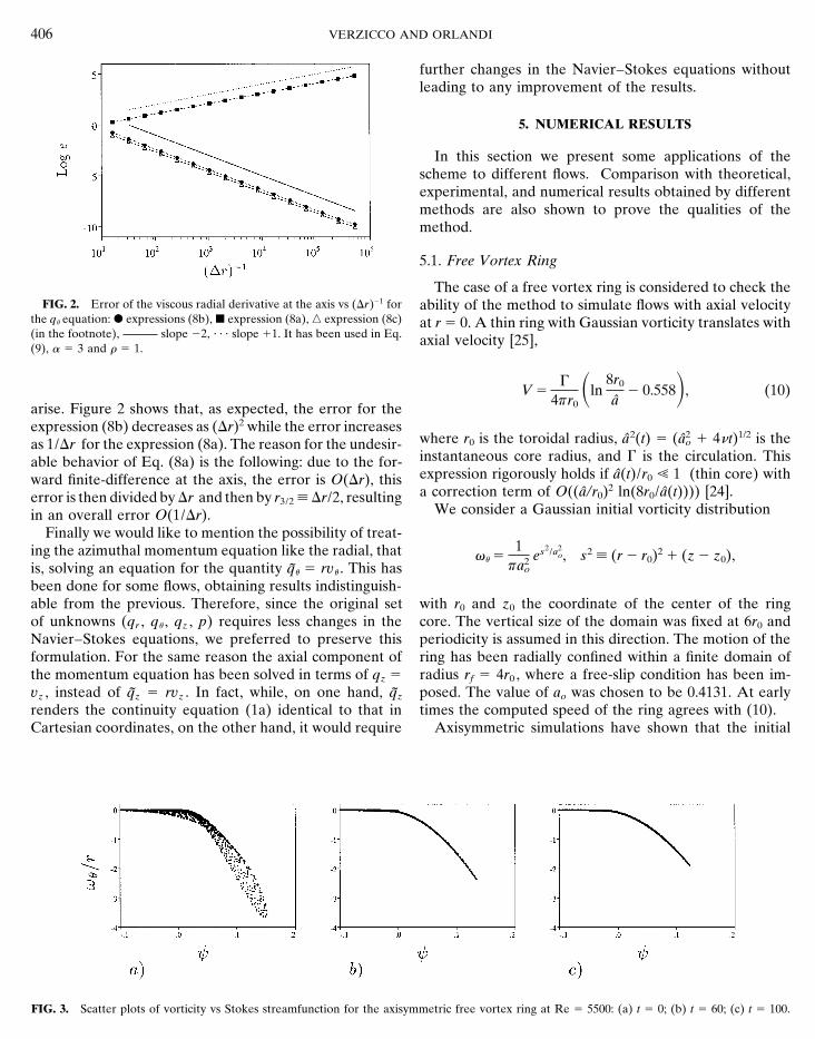
The case of a free vortex ring is considered to check theFIG. 2. Error of the viscous radial derivative at the axis vs (Dr)21 for ability of the method to simulate flows with axial velocity

the qu equation: d expressions (8b), j expression (8a), n expression (8c) at r 5 0. A thin ring with Gaussian vorticity translates with(in the footnote), slope 22, ? ? ? slope 11. It has been used in Eq. axial velocity [25],(9), a 5 3 and r 5 1.

V 5G

4fr0Sln

8r0

a2 0.558D, (10)

arise. Figure 2 shows that, as expected, the error for theexpression (8b) decreases as (Dr)2 while the error increases

where r0 is the toroidal radius, a2(t) 5 (a2o 1 4nt)1/2 is theas 1/Dr for the expression (8a). The reason for the undesir-

instantaneous core radius, and G is the circulation. Thisable behavior of Eq. (8a) is the following: due to the for-expression rigorously holds if a(t)/r0 ! 1 (thin core) withward finite-difference at the axis, the error is O(Dr), thisa correction term of O((a/r0)2 ln(8r0/a(t)))) [24].error is then divided by Dr and then by r3/2 ; Dr/2, resulting

We consider a Gaussian initial vorticity distributionin an overall error O(1/Dr).Finally we would like to mention the possibility of treat-

ing the azimuthal momentum equation like the radial, that gu 51

fa2o

es2/a2o, s2 ; (r 2 r0)2 1 (z 2 z0),

is, solving an equation for the quantity qu 5 rvu . This hasbeen done for some flows, obtaining results indistinguish-able from the previous. Therefore, since the original set with r0 and z0 the coordinate of the center of the ring

core. The vertical size of the domain was fixed at 6r0 andof unknowns (qr , qu , qz , p) requires less changes in theNavier–Stokes equations, we preferred to preserve this periodicity is assumed in this direction. The motion of the

ring has been radially confined within a finite domain offormulation. For the same reason the axial component ofthe momentum equation has been solved in terms of qz 5 radius rf 5 4r0 , where a free-slip condition has been im-

posed. The value of ao was chosen to be 0.4131. At earlyvz , instead of qz 5 rvz . In fact, while, on one hand, qz

renders the continuity equation (1a) identical to that in times the computed speed of the ring agrees with (10).Axisymmetric simulations have shown that the initialCartesian coordinates, on the other hand, it would require

FIG. 3. Scatter plots of vorticity vs Stokes streamfunction for the axisymmetric free vortex ring at Re 5 5500: (a) t 5 0; (b) t 5 60; (c) t 5 100.

3D INCOMPRESSIBLE FLOWS 407

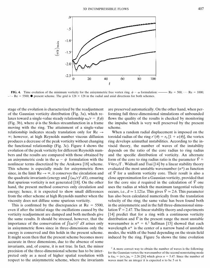
FIG. 4. Time evolution of the minimum vorticity for the axisymmetric free vortex ring. c 2 g formulation: Re 5 500; ? ? ? Re 5 1000;– ? – Re 5 5500; d present scheme. The grid is 128 3 128 in the radial and axial directions for both schemes.

stage of the evolution is characterized by the readjustment are preserved automatically. On the other hand, when per-forming full three-dimensional simulations of unboundedof the Gaussian vorticity distribution (Fig. 3a), which re-

laxes toward a single-value steady relationship gu/r 5 f(c) flows the quality of the results is checked by monitoringthe impulse which is very well preserved by the present(Fig. 3b), where c is the Stokes streamfunction in a frame

moving with the ring. The attainment of a single-value scheme.When a random radial displacement is imposed on therelationship indicates steady translation only for Re R

y; however, at high Reynolds number viscous diffusion toroidal radius of the ring r9(u) 5 r0 [1 1 «(u)], the vortexring develops azimuthal instabilities. According to the in-produces a decrease of the peak vorticity without changing

the functional relationship (Fig. 3c). Figure 4 shows the viscid theory, the number of waves of the instabilitydepends on the ratio of the core radius to ring radiusevolution of the peak vorticity for different Reynolds num-

bers and the results are compared with those obtained by and the specific distribution of vorticity. An alternateform of the core to ring radius ratio is the parameter V 5

.an axisymmetric code in the g 2 c formulation with thenonlinear terms discretized by the Arakawa [18] scheme. V4fr0/G . Widnall and Tsai [14] by a linear stability theory

evaluated the most unstable wavenumber (n*) as functionThis scheme is especially made for axisymmetric flowssince, in the limit Re R y, it conserves the circulation and of V for a uniform vorticity core. Their result is also a

close approximation for a Gaussian vorticity, provided thatthe quadratic invariants (energy and e(gu/r)2 dS), ensuringthat spurious vorticity is not generated [18]. On the other for the core size a required in the calculation of V one

uses the radius at which the maximum tangential velocityhand, the present method conserves only circulation andenergy; hence, it is expected to show small differences occurs, i.e., a Q 1.121a. This gives V Q 2.6. This parameter

has also been calculated numerically from the translationfrom the other scheme at high Reynolds number when theviscosity does not diffuse some spurious vorticity. velocity of the ring; the same value has been found both

in the axisymmetric and in the full three-dimensional simu-This is confirmed by the discrepancies at Re 5 5500,even if after the initial stage the oscillations caused by the lation V 5 2.47. The linear stability theory and experiments

[14] predict that for a ring with a continuous vorticityvorticity readjustment are damped and both methods givethe same results. It should be stressed, however, that the distribution and V in the present range the most unstable

wavenumber is n* 5 6.2 Saffman [15] showed that eachimportance of the conservation of e(g/r)2 dS arises onlyin axisymmetric flows since in three-dimensions only the wavelength n* is the center of a narrow band of unstable

modes, the width of the band depending on the strain fieldenergy is conserved and this holds in the present scheme.It might seem then that the present scheme becomes more induced by the ring. Figure 5a shows the time evolutionaccurate in three dimensions, due to the absence of someinvariants, and, of course, it is not true. In fact, the minor

2 A more correct way to obtain the number of waves is the following:precision of the three-dimensional scheme has to be inter- for the Gaussian vortex the wavenumber of the second nonrotating modepreted only as a need of higher spatial resolution with is ka0 5 (n/ro)a0 5 2.26 [26] which gives n 5 5.47. Since the number of

waves must be an integer it is expected n to be 5 or 6.respect to the axisymmetric scheme, where the invariants

408 VERZICCO AND ORLANDI

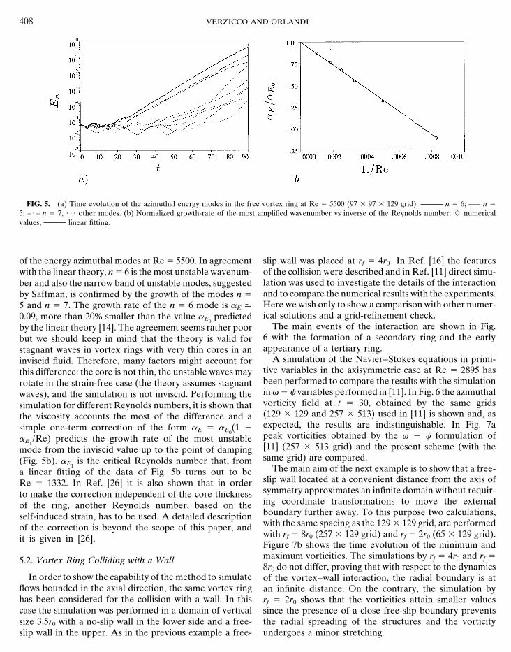
FIG. 5. (a) Time evolution of the azimuthal energy modes in the free vortex ring at Re 5 5500 (97 3 97 3 129 grid): n 5 6; ––– n 5

5; – ? – n 5 7, ? ? ? other modes. (b) Normalized growth-rate of the most amplified wavenumber vs inverse of the Reynolds number: L numericalvalues; linear fitting.

of the energy azimuthal modes at Re 5 5500. In agreement slip wall was placed at rf 5 4r0 . In Ref. [16] the featuresof the collision were described and in Ref. [11] direct simu-with the linear theory, n 5 6 is the most unstable wavenum-lation was used to investigate the details of the interactionber and also the narrow band of unstable modes, suggestedand to compare the numerical results with the experiments.by Saffman, is confirmed by the growth of the modes n 5Here we wish only to show a comparison with other numer-5 and n 5 7. The growth rate of the n 5 6 mode is aE Qical solutions and a grid-refinement check.0.09, more than 20% smaller than the value aE0

predictedThe main events of the interaction are shown in Fig.by the linear theory [14]. The agreement seems rather poor

6 with the formation of a secondary ring and the earlybut we should keep in mind that the theory is valid forappearance of a tertiary ring.stagnant waves in vortex rings with very thin cores in an

A simulation of the Navier–Stokes equations in primi-inviscid fluid. Therefore, many factors might account fortive variables in the axisymmetric case at Re 5 2895 hasthis difference: the core is not thin, the unstable waves maybeen performed to compare the results with the simulationrotate in the strain-free case (the theory assumes stagnantin g 2 c variables performed in [11]. In Fig. 6 the azimuthalwaves), and the simulation is not inviscid. Performing thevorticity field at t 5 30, obtained by the same gridssimulation for different Reynolds numbers, it is shown that(129 3 129 and 257 3 513) used in [11] is shown and, asthe viscosity accounts the most of the difference and aexpected, the results are indistinguishable. In Fig. 7asimple one-term correction of the form aE 5 aE0

(1 2peak vorticities obtained by the g 2 c formulation ofaE1

/Re) predicts the growth rate of the most unstable[11] (257 3 513 grid) and the present scheme (with themode from the inviscid value up to the point of dampingsame grid) are compared.(Fig. 5b). aE1

is the critical Reynolds number that, fromThe main aim of the next example is to show that a free-a linear fitting of the data of Fig. 5b turns out to be

slip wall located at a convenient distance from the axis ofRe 5 1332. In Ref. [26] it is also shown that in ordersymmetry approximates an infinite domain without requir-to make the correction independent of the core thicknessing coordinate transformations to move the externalof the ring, another Reynolds number, based on theboundary further away. To this purpose two calculations,self-induced strain, has to be used. A detailed descriptionwith the same spacing as the 129 3 129 grid, are performedof the correction is beyond the scope of this paper, andwith rf 5 8r0 (257 3 129 grid) and rf 5 2r0 (65 3 129 grid).it is given in [26].Figure 7b shows the time evolution of the minimum andmaximum vorticities. The simulations by rf 5 4r0 and rf 55.2. Vortex Ring Colliding with a Wall8r0 do not differ, proving that with respect to the dynamics

In order to show the capability of the method to simulate of the vortex–wall interaction, the radial boundary is atflows bounded in the axial direction, the same vortex ring an infinite distance. On the contrary, the simulation byhas been considered for the collision with a wall. In this rf 5 2r0 shows that the vorticities attain smaller valuescase the simulation was performed in a domain of vertical since the presence of a close free-slip boundary prevents

the radial spreading of the structures and the vorticitysize 3.5r0 with a no-slip wall in the lower side and a free-slip wall in the upper. As in the previous example a free- undergoes a minor stretching.

3D INCOMPRESSIBLE FLOWS 409

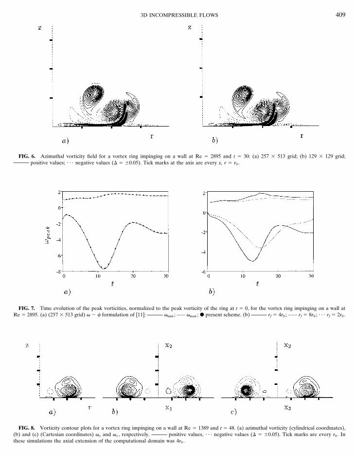
FIG. 6. Azimuthal vorticity field for a vortex ring impinging on a wall at Re 5 2895 and t 5 30: (a) 257 3 513 grid; (b) 129 3 129 grid;positive values; ? ? ? negative values (D 5 60.05). Tick marks at the axis are every x, r 5 r0 .

FIG. 7. Time evolution of the peak vorticities, normalized to the peak vorticity of the ring at t 5 0, for the vortex ring impinging on a wall atRe 5 2895. (a) (257 3 513 grid) g 2 c formulation of [11]: gmin ; ––– gmax ; d present scheme. (b) rf 5 4r0 ; ––– rf 5 8r0 ; ? ? ? rf 5 2r0 .

FIG. 8. Vorticity contour plots for a vortex ring impinging on a wall at Re 5 1389 and t 5 48. (a) azimuthal vorticity (cylindrical coordinates),(b) and (c) (Cartesian coordinates) gx and gz , respectively. positive values, ? ? ? negative values (D 5 60.05). Tick marks are every r0 . Inthese simulations the axial extension of the computational domain was 4r0 .

410 VERZICCO AND ORLANDI

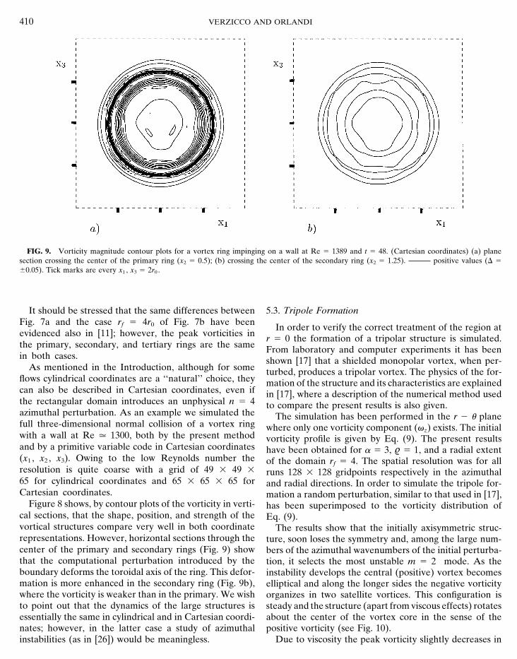
FIG. 9. Vorticity magnitude contour plots for a vortex ring impinging on a wall at Re 5 1389 and t 5 48. (Cartesian coordinates) (a) planesection crossing the center of the primary ring (x2 5 0.5); (b) crossing the center of the secondary ring (x2 5 1.25). positive values (D 5

60.05). Tick marks are every x1 , x3 5 2r0 .

It should be stressed that the same differences between 5.3. Tripole FormationFig. 7a and the case rf 5 4r0 of Fig. 7b have been In order to verify the correct treatment of the region atevidenced also in [11]; however, the peak vorticities in r 5 0 the formation of a tripolar structure is simulated.the primary, secondary, and tertiary rings are the same From laboratory and computer experiments it has beenin both cases. shown [17] that a shielded monopolar vortex, when per-

As mentioned in the Introduction, although for some turbed, produces a tripolar vortex. The physics of the for-flows cylindrical coordinates are a ‘‘natural’’ choice, they mation of the structure and its characteristics are explainedcan also be described in Cartesian coordinates, even if in [17], where a description of the numerical method usedthe rectangular domain introduces an unphysical n 5 4 to compare the present results is also given.azimuthal perturbation. As an example we simulated the The simulation has been performed in the r 2 u planefull three-dimensional normal collision of a vortex ring where only one vorticity component (gz) exists. The initialwith a wall at Re Q 1300, both by the present method vorticity profile is given by Eq. (9). The present resultsand by a primitive variable code in Cartesian coordinates have been obtained for a 5 3, % 5 1, and a radial extent(x1 , x2 , x3). Owing to the low Reynolds number the of the domain rf 5 4. The spatial resolution was for allresolution is quite coarse with a grid of 49 3 49 3 runs 128 3 128 gridpoints respectively in the azimuthal65 for cylindrical coordinates and 65 3 65 3 65 for and radial directions. In order to simulate the tripole for-Cartesian coordinates. mation a random perturbation, similar to that used in [17],

Figure 8 shows, by contour plots of the vorticity in verti- has been superimposed to the vorticity distribution ofcal sections, that the shape, position, and strength of the Eq. (9).vortical structures compare very well in both coordinate The results show that the initially axisymmetric struc-representations. However, horizontal sections through the ture, soon loses the symmetry and, among the large num-center of the primary and secondary rings (Fig. 9) show bers of the azimuthal wavenumbers of the initial perturba-that the computational perturbation introduced by the tion, it selects the most unstable m 5 2 mode. As theboundary deforms the toroidal axis of the ring. This defor- instability develops the central (positive) vortex becomesmation is more enhanced in the secondary ring (Fig. 9b), elliptical and along the longer sides the negative vorticitywhere the vorticity is weaker than in the primary. We wish organizes in two satellite vortices. This configuration isto point out that the dynamics of the large structures is steady and the structure (apart from viscous effects) rotatesessentially the same in cylindrical and in Cartesian coordi- about the center of the vortex core in the sense of the

positive vorticity (see Fig. 10).nates; however, in the latter case a study of azimuthalinstabilities (as in [26]) would be meaningless. Due to viscosity the peak vorticity slightly decreases in

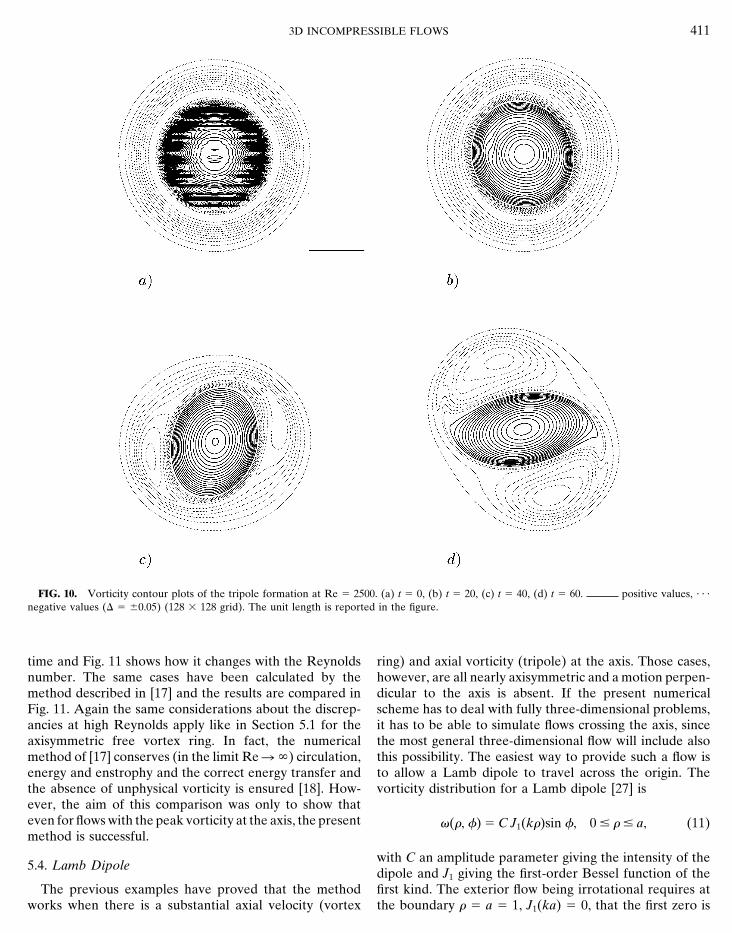
3D INCOMPRESSIBLE FLOWS 411

FIG. 10. Vorticity contour plots of the tripole formation at Re 5 2500. (a) t 5 0, (b) t 5 20, (c) t 5 40, (d) t 5 60. positive values, ? ? ?

negative values (D 5 60.05) (128 3 128 grid). The unit length is reported in the figure.

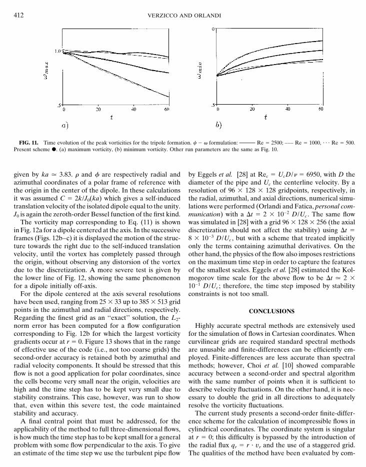
time and Fig. 11 shows how it changes with the Reynolds ring) and axial vorticity (tripole) at the axis. Those cases,however, are all nearly axisymmetric and a motion perpen-number. The same cases have been calculated by the

method described in [17] and the results are compared in dicular to the axis is absent. If the present numericalscheme has to deal with fully three-dimensional problems,Fig. 11. Again the same considerations about the discrep-

ancies at high Reynolds apply like in Section 5.1 for the it has to be able to simulate flows crossing the axis, sincethe most general three-dimensional flow will include alsoaxisymmetric free vortex ring. In fact, the numerical

method of [17] conserves (in the limit Re R y) circulation, this possibility. The easiest way to provide such a flow isto allow a Lamb dipole to travel across the origin. Theenergy and enstrophy and the correct energy transfer and

the absence of unphysical vorticity is ensured [18]. How- vorticity distribution for a Lamb dipole [27] isever, the aim of this comparison was only to show thateven for flows with the peak vorticity at the axis, the present g(r, f) 5 C J1(kr)sin f, 0 # r # a, (11)method is successful.

with C an amplitude parameter giving the intensity of the5.4. Lamb Dipole

dipole and J1 giving the first-order Bessel function of thefirst kind. The exterior flow being irrotational requires atThe previous examples have proved that the method

works when there is a substantial axial velocity (vortex the boundary r 5 a 5 1, J1(ka) 5 0, that the first zero is

412 VERZICCO AND ORLANDI

FIG. 11. Time evolution of the peak vorticities for the tripole formation. c 2 g formulation: Re 5 2500; ––– Re 5 1000, ? ? ? Re 5 500.Present scheme d. (a) maximum vorticity, (b) minimum vorticity. Other run parameters are the same as Fig. 10.

given by ka Q 3.83. r and f are respectively radial and by Eggels et al. [28] at Rec 5 UcD/n 5 6950, with D thediameter of the pipe and Uc the centerline velocity. By aazimuthal coordinates of a polar frame of reference with

the origin in the center of the dipole. In these calculations resolution of 96 3 128 3 128 gridpoints, respectively, inthe radial, azimuthal, and axial directions, numerical simu-it was assumed C 5 2k/J0(ka) which gives a self-induced

translation velocity of the isolated dipole equal to the unity. lations were performed (Orlandi and Fatica, personal com-munication) with a Dt 5 2 3 1022 D/Uc . The same flowJ0 is again the zeroth-order Bessel function of the first kind.

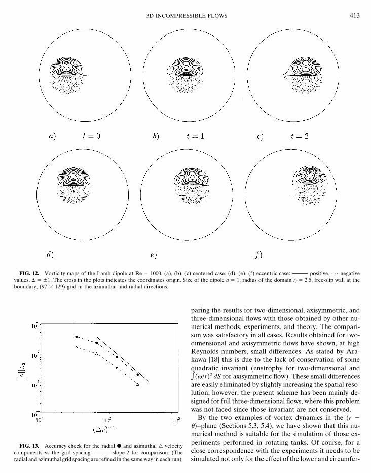
The vorticity map corresponding to Eq. (11) is shown was simulated in [28] with a grid 96 3 128 3 256 (the axialdiscretization should not affect the stability) using Dt 5in Fig. 12a for a dipole centered at the axis. In the successive

frames (Figs. 12b–c) it is displayed the motion of the struc- 8 3 1023 D/Uc , but with a scheme that treated implicitlyonly the terms containing azimuthal derivatives. On theture towards the right due to the self-induced translation

velocity, until the vortex has completely passed through other hand, the physics of the flow also imposes restrictionson the maximum time step in order to capture the featuresthe origin, without observing any distorsion of the vortex

due to the discretization. A more severe test is given by of the smallest scales. Eggels et al. [28] estimated the Kol-mogorov time scale for the above flow to be Dt Q 2 3the lower line of Fig. 12, showing the same phenomenon

for a dipole initially off-axis. 1021 D/Uc ; therefore, the time step imposed by stabilityconstraints is not too small.For the dipole centered at the axis several resolutions

have been used, ranging from 25 3 33 up to 385 3 513 gridpoints in the azimuthal and radial directions, respectively. CONCLUSIONSRegarding the finest grid as an ‘‘exact’’ solution, the L2-norm error has been computed for a flow configuration Highly accurate spectral methods are extensively used

for the simulation of flows in Cartesian coordinates. Whencorresponding to Fig. 12b for which the largest vorticitygradients occur at r 5 0. Figure 13 shows that in the range curvilinear grids are required standard spectral methods

are unusable and finite-differences can be efficiently em-of effective use of the code (i.e., not too coarse grids) thesecond-order accuracy is retained both by azimuthal and ployed. Finite-differences are less accurate than spectral

methods; however, Choi et al. [10] showed comparableradial velocity components. It should be stressed that thisflow is not a good application for polar coordinates, since accuracy between a second-order and spectral algorithm

with the same number of points when it is sufficient tothe cells become very small near the origin, velocities arehigh and the time step has to be kept very small due to describe velocity fluctuations. On the other hand, it is nec-

essary to double the grid in all directions to adequatelystability constrains. This case, however, was run to showthat, even within this severe test, the code maintained resolve the vorticity fluctuations.

The current study presents a second-order finite-differ-stability and accuracy.A final central point that must be addressed, for the ence scheme for the calculation of incompressible flows in

cylindrical coordinates. The coordinate system is singularapplicability of the method to full three-dimensional flows,is how much the time step has to be kept small for a general at r 5 0; this difficulty is bypassed by the introduction of

the radial flux qr 5 r ? vr and the use of a staggered grid.problem with some flow perpendicular to the axis. To givean estimate of the time step we use the turbulent pipe flow The qualities of the method have been evaluated by com-

3D INCOMPRESSIBLE FLOWS 413

FIG. 12. Vorticity maps of the Lamb dipole at Re 5 1000. (a), (b), (c) centered case, (d), (e), (f) eccentric case: positive, ? ? ? negativevalues, D 5 61. The cross in the plots indicates the coordinates origin. Size of the dipole a 5 1, radius of the domain rf 5 2.5, free-slip wall at theboundary, (97 3 129) grid in the azimuthal and radial directions.

paring the results for two-dimensional, axisymmetric, andthree-dimensional flows with those obtained by other nu-merical methods, experiments, and theory. The compari-son was satisfactory in all cases. Results obtained for two-dimensional and axisymmetric flows have shown, at highReynolds numbers, small differences. As stated by Ara-kawa [18] this is due to the lack of conservation of somequadratic invariant (enstrophy for two-dimensional ande(g/r)2 dS for axisymmetric flow). These small differencesare easily eliminated by slightly increasing the spatial reso-lution; however, the present scheme has been mainly de-signed for full three-dimensional flows, where this problemwas not faced since those invariant are not conserved.

By the two examples of vortex dynamics in the (r 2u)–plane (Sections 5.3, 5.4), we have shown that this nu-merical method is suitable for the simulation of those ex-periments performed in rotating tanks. Of course, for aFIG. 13. Accuracy check for the radial d and azimuthal n velocityclose correspondence with the experiments it needs to becomponents vs the grid spacing. slope-2 for comparison. (The

radial and azimuthal grid spacing are refined in the same way in each run). simulated not only for the effect of the lower and circumfer-

414 VERZICCO AND ORLANDI

Spaziale Italiana’’ under Contract ASI92RS27/141ATD. The preliminaryential solid boundaries (already possible by the presentresults of this work were presented at the ICOSAHOM 1992, Montpelier,scheme), but also for the upper free surface. For low rota-France. Finally, the authors thank the referee III for suggesting the

tion rates of the tank the free surface can be easily approxi- simulation of the Lamb dipole.mated by a rigid free-slip wall. On the contrary, for highrotation rates the deformations of the surface become im-portant and these would require much more work.

REFERENCES

APPENDIX 1. A. Wray and Y. Hussaini, AIAA Paper 80-0275, Pasadena, CA,1980 (unpublished).

A1. Boundary Conditions 2. P. Moin and J. Kim, J. Fluid Mech. 118, 159 (1982).

3. M. M. Rogers, and R. D. Moser, J. Fluid Mech. 243, 183 (1992).In Section 3 it has been mentioned that ql11i 5 qi 1

4. V. M. Melander, F. Hussain, and A. Basu, ‘‘Breakdown of a CircularO(Dt2). To prove this statement we follow the procedureJet into Turbulence,’’ in Proceedings, 8th Symp. on Turb. Shear Flows,

described in [21]. Regarding qi as an approximation to the Munich, 1991 (unpublished).quantity q*i , continuous in time, it is required that q*i satisfy 5. S. K. Stanaway, B. J. Cantwell, and P. R. Spalart, Ph.D. thesis, NASAthe conditions TM 101041, 1988 (unpublished).

6. A. Leonard and A. Wray, ‘‘A New Numerical Method for theSimulation of Three-Dimensional Flow in a Pipe,’’ in Fourth Int.Conf. on Numer. Methods in Fluid Dyn., Colorado, Lecture Notes

­q*i­t

5 2Gi p* 1 H*i 11

ReAiq*i ,

in Physics, Vol. 135, p. 335 (Springer-Verlag, New York, 1975).

7. J. C. Buell and I. Catton, J. Heat Transfer 105, 255 (1983).q l11

i 5 q*i (tl11), p l11 5 p*(tl11),8. J. G. M. Eggels, Ph.D. thesis, Delft University of Tech., 1994 (unpub-

lished).where for brevity it has been indicated by Ai , the operator 9. M. M. Rai, and P. Moin, J. Comput. Phys. 96, 15 (1991).for the viscous terms (Ai 5 Aiu 1 Air 1 Aiz) of Eq. (1a). 10. H. Choi, P. Moin, and J. Kim, Ph.D. thesis TF-55, Stanford University,For the generic time step we can write 1992 (unpublished).

11. P. Orlandi and R. Verzicco, J. Fluid Mech. 256, 615 (1993).

12. R. Verzicco and P. Orlandi, Phys. Fluids 6, 751 (1994).qi P q*i (tl11) 5 q*i (tl) 1

­q*i­t U

tl

Dt 1 O((Dt)2) 13. U. Schumann, J. Comput. Phys. 18, 376 (1975).

14. S. E. Widnall and C. Y. Tsai, Phil. Trans. R. Soc. London A 287,273 (1977).

15. P. G. Saffman, J. Fluid Mech. 84, 625 (1978).5 q*i (tl) 1 S2Gip* 1 H*i 11R

Aiq*i D Utl

Dt 1 O((Dt)2).16. J. D. A. Walker, C. R. Smith, A. W. Cerra, and J. L. Doligaski,

J. Fluid Mech. 181, 99 (1987).

17. P. Orlandi and G. J. F. van Heijst, Fluid Dyn. Res. 9, 179 (1992).Since ql11i 5 q*i (tl11) and pl11 5 p*(tl11) it follows that

18. A. Arakawa, J. Comput. Phys. 1, 119 (1966).

19. A. Grammelvedt, Mon. Weather Rev. 97(5), 384 (1969).qi 5 ql

i 1 S2Gipl 1 Hli 1

1Re

AiqliD Dt 1 O((Dt)2) 20. K. Horiuti, J. Comput. Phys. 71, 343 (1987).

21. J. Kim and P. Moin, J. Comput. Phys. 59, 308 (1985).

22. R. M. Beam and R. F. Warming, J. Comput. Phys. 22, 875 ql

i 1­qi

­t Utl

Dt 1 O((Dt)2), (1976).

23. P. R. Spalart, R. D. Moser, and M. M. Rogers, J. Comput. Phys. 96,297 (1991).

24. L. E. Fraenkel, J. Fluid Mech. 51, 119 (1972).so that25. P. G. Saffman, Stud. Appl. Math. 49(4), 371 (1970).

26. K. Shariff, R. Verzicco, and P. Orlandi, J. Fluid Mech. 279, 351qi 5 ql11i 1 O((Dt)2).

(1994).

27. Sir H. Lamb, Hydrodynamics (Dover, New York, 1932).ACKNOWLEDGMENTS28. J. G. M. Eggels, F. Unger, M. H. Weiss, J. Westerweel, R. T.

Adrian, R. Friedrich, and F. T. M. Nieuwstadt, J. Fluid Mech. 268,The authors express their gratitude to Dr. M. Fatica and Dr. K. Shariff175 (1994).for useful discussions. The research was supported by a grant ‘‘Agenzia