HAL Id: hal-02997074https://hal.archives-ouvertes.fr/hal-02997074

Submitted on 9 Nov 2020

HAL is a multi-disciplinary open accessarchive for the deposit and dissemination of sci-entific research documents, whether they are pub-lished or not. The documents may come fromteaching and research institutions in France orabroad, or from public or private research centers.

L’archive ouverte pluridisciplinaire HAL, estdestinée au dépôt et à la diffusion de documentsscientifiques de niveau recherche, publiés ou non,émanant des établissements d’enseignement et derecherche français ou étrangers, des laboratoirespublics ou privés.

A finite-element algorithm for Stokes flow through oiland gas production tubing of uniform diameter

Lateef T. Akanji, Joao Chidamoio

To cite this version:Lateef T. Akanji, Joao Chidamoio. A finite-element algorithm for Stokes flow through oil and gasproduction tubing of uniform diameter. Oil & Gas Science and Technology - Revue d’IFP Energiesnouvelles, Institut Français du Pétrole, 2020, 75, pp.79. �10.2516/ogst/2020067�. �hal-02997074�

A finite-element algorithm for Stokes flow through oil and gasproduction tubing of uniform diameterLateef T. Akanji1,* and Joao Chidamoio2

1 School of Engineering, University of Aberdeen, AB24 3FX Aberdeen, UK2Department of Chemical Engineering, Faculty of Engineering, Eduardo Mondlane University, 257 Maputo, Mozambique

Received: 16 February 2020 / Accepted: 28 August 2020

Abstract. Stokes flow of a Newtonian fluid through oil and gas production tubing of uniform diameter isstudied. Using a direct simulation on computer-aided design of discretised conduits, velocity profiles withgravitational effect and pressure fields are obtained for production tubing of different inner but uniformdiameter. The results obtained with this new technique are compared with the integrated form of the Hagen–Poiseuille equation (i.e., lubrication approximation) and data obtained from experimental and numerical studiesfor flow in vertical pipes. Good agreement is found in the creeping flow regime between the computed and mea-sured pressure fields with a coefficient of correlation of 0.97. Further, computed velocity field was benchmarkedagainstANSYS Fluent; a finite element commercial software package, in a single-phase flow simulation using theaxial velocity profile computed at predefined locations along the geometric domains. This method offers animproved solution approach over other existing methods both in terms of computational speed and accuracy.

Nomenclature

V Volume, m3

F Right-hand termN Interpolation functionP Pressure, PaW Weighting functionl Fluid viscosity, Pa sw Parabolic functionq Density, kg/m3

x Domain boundaryn̂ Unit normal to the boundaryg Acceleration due to gravity, m/s2

U Fluid velocity, m/sh Maximum width of geometry, mL Length of geometry, mD Diameter of geometry, me Flow field mismatch

Subscript

x, y, z Directions

Superscript

T Matrix transposee Element

1 Introduction

Fluid flow through pipes has attracted a great deal of scien-tific and engineering discipline interests due to their preva-lence in biological systems such as blood flow in humanbody and multi-phase in flow in oil and gas producing wells.Flow in porous media is often modelled as periodicallyassembled tubes (e.g., Galdi and Robertson [1], Lahbabiand Chang [2], Bernabé and Olson [3], Payatakes et al.[4, 5]). In this case, the total pore-space can be representedby a network of tubes with each tube being assigned ahydraulic conductance C, defined by analogy with the elec-trical conductance [6]. In oilfield applications, severalauthors have studied the effect of production tubingdiameter on oil production and vertical lift performance(e.g., Chidamoio et al. [7]). Hernandez [8] reported thatlarge production tubing found in old oil fields where reser-voir pressure has declined to very low values may bereplaced by small diameter tubing in order to produce ata stable rate.

Several solutions exist for creeping flow of a Newtonianfluid through vertical pipes. Approximate solutions havebeen obtained using the Hagen–Poiseuille (i.e., lubricationapproximation) for flow in pipes by integrating theequation at each axial location along the pipe to obtainthe overall pressure drop (e.g., Al-Atabi et al. [9]). Thishas allowed for modelling and simulation of Newtonianand non-Newtonian fluid flow in networks of interconnectedpipes for oil transportation, production tubing design or a* Corresponding author: l.akanji@abdn.ac.uk

This is an Open Access article distributed under the terms of the Creative Commons Attribution License (https://creativecommons.org/licenses/by/4.0),which permits unrestricted use, distribution, and reproduction in any medium, provided the original work is properly cited.

Oil & Gas Science and Technology – Rev. IFP Energies nouvelles 75, 79 (2020) Available online at:�L.T. Akanji & J. Chidamoio, published by IFP Energies nouvelles, 2020 ogst.ifpenergiesnouvelles.fr

https://doi.org/10.2516/ogst/2020067

REGULAR ARTICLEREGULAR ARTICLE

simplified model of porous media (e.g., Al-Atabi et al. [10],Sochi [11], Sabooniha et al. [12]). Navier–Stokes equationhas also been applied using analytical methods such asasymptotic series solution (e.g., Sisavath et al. [13]) andnumerical methods such as the collocation method (e.g.,Tilton and Payatakes [14]), geometric iteration method(e.g., Deiber and Schowalter [15]) and the boundary inte-gral method (e.g., Hemmat and Borhan [16]).

Although, results obtained from analytical solutions tothe Navier–Stokes equation generally offer improvementover the lubrication approximation with regard to thedetails of the flow field, numerical approaches are preferablein cases where detailed flow structure is desired [13]. Numer-ical methods are usually in good agreement with experimen-tal data and have generally produced very good results.However, computational costs may be prohibitively high.

The Direct Numerical Simulation (DNS) methods havebeen used to obtain accurate turbulent flow field in a pipe(e.g. Sirisup et al. [17] Ge and Xu [18], Ould-Rouiss et al.[19], Tamano et al. [20], Zhu et al. [21], Li et al. [22, 23]).Ge and Xu [18] developed a numerical scheme capable ofextending the scope of the spectral method without solvingthe covariant and contravariant forms of the Navier–Stokesequations in the curvilinear coordinates. They representedthe primitive variables by the Fourier series and theChebyshev polynomials in the computational space.Li et al. [22] used an explicit coupling scheme betweenparticles and the fluid, which considers two-way couplingbetween the particle and the fluid for the investigation ofparticle-laden turbulent flows in low Reynolds numberaxisymmetric jet. Zhu et al. [21] concluded that the sub-gridscale model may be neglected at a spatial resolution of about106 and a duct flow at the particular friction Reynoldsnumber of 600 will be appropriate. Laboratory experimentsusually give a detailed structural behaviour of flow in pro-duction tubing, but, numerical approaches are cheaperand preferable in preliminary investigation and analysis.

These aforementioned DNS methods have focussedmainly on the modelling of flow structure and less on theactual engineering of the physical problem particularly inthe numerical evaluation of the velocity fields within realis-tic geometries. Further, numerical computation on realisticrepresentation of geometric entities is still a challenge.Commercial software packages (such as ANSYS Fluent)and some other open-source applications are used in numer-ical simulation of Stokes flow in pipes. However, there aresignificant limitations in such computation on representa-tive oil and gas production tubing discretised with millionsof finite-elements. Such investigations are important giventhat production tubing is usually completed in productioncasing or liner perforated for oil and gas production fromhydrocarbon reservoirs where inflow performance is evalu-ated. Such production tubing systems may also have gas-liftmandrels which have to be incorporated in the numericalmodel design and computation. The workflow developedherein aims to proffer solution to this problem. The work-flow allows for detailed flow structure; a caveat in theanalytical solutions approach, to be captured whilst provid-ing an opportunity to simulate flow directly on physical rep-resentation of long production tubing where computational

speed is desirable. In this work, flow simulation is conductedon physical geometric models of production tubing ofvarying diameters using Computer-Aided Design (CAD)models. The CAD models are constructed with Non-Uniform Rational B-Spline (NURBS) curves and surfacesof order 3, capable of capturing curvatures with tolerance-based level of detail. Geometries are meshed using unstruc-tured spatially variable adaptive grid, tracking free-formentities such as NURBS. Stokes flow simulation are thenconducted on production tubing of different diameters tocompute pressure and associated velocity fields respectively.Computation is implemented in complex systems mod-elling platform (CSMP++); an application programmerinterface engineered in ANSI/ISOC++. The developedmodel is verified against analytical solution and thenvalidated against experimental and numerical results.

2 Methodology

A FEM-based algorithm for Stokes flow in productiontubing is formulated by solving the discretised equationusing an Algebraic MultiGrid Solver (SAMG); an efficientlinear solver library based on algebraic multigrid system[24]. The workflow involves: (i) building the geometricmodel with CAD in 2D and 3D domains, (ii) meshing thegeometric samples using unstructured mesh consisting ofline, triangle and tetrahedron elements, (iii) assigningboundary and initial conditions, (iv) discretising the flowequations, (v) solving equations using algebraic multigridsolver and, (vi) post-processing and model visualisation.A flowchart for the computational approach developed inthis work is shown in Figure 1.

2.1 Governing equations

The flow of fluid in a pipe can be described by the generalform of the momentum equation, constrained by the massconservation equation. The momentum equation can bewritten as:

oot

qUð Þ|fflfflfflffl{zfflfflfflffl}a

þr: qUUð Þ|fflfflfflfflfflffl{zfflfflfflfflfflffl}b

¼ � rp|{z}c

þ r � s|ffl{zffl}d

þ qg|{z}e

; ð1Þ

where, q and U are the density and velocity respectively.In equation (1), the term a represents the rate of incre-ment in momentum per unit volume; b is the change inmomentum due to convection; c is the pressure gradient;d represents the viscous and turbulent contributions; e isthe gravitational forces. The mass conservation equationcan be expressed as:

oqot

þr � qUð Þ ¼ 0: ð2ÞIn this investigation, the pipe fluid pressure is computedand compared with analytical solutions and data obtainedfrom laboratory measurements. Furthermore, flow isassumed incompressible and Newtonian, thus:

qoUot

þ qU � rU ¼ �rpþ qg~eþ lr2U: ð3Þ

L.T. Akanji and J. Chidamoio: Oil & Gas Science and Technology – Rev. IFP Energies nouvelles 75, 79 (2020)2

The fully developed flow is assumed to be achieved when theinertia term is small compared to the viscous term; lowReynolds number Re ¼ qUL

d (e.g., Guet et al. [25], Batchelor[26], Akanji andMatthai [27]), hence, the inertia term can beignored and equation (3) can be rewritten as:

qoUot

¼ �rP þ lr2U; ð4Þ

where,

rP ¼ rp� qg~e; ð5Þis the reduced pressure gradient. We consider a steady-state flow in the production tubing where at any fixed

point in space, the velocity does not vary with time; henceignoring transient effects and assuming that the fluiddensity is constant, equation (4) reduces to the Stokesequation. Thus the momentum and mass conservationequations can be written as:

lr2U ¼ rP; ð6Þr �U ¼ 0: ð7Þ

In computational fluid mechanics, the correct choice of theshape functions for velocity and pressure can be adjusted inthe case of an isothermal and incompressible flow throughthe inf-sup compatibility condition of the Ladyzhenskaya–Babuska–Brezzi (LBB condition) [28]. The equivalence of

Fig. 1. Flowchart for model construction, FEM meshing and numerical computation of fluid pressure and velocity fields in geometricconduits. Geometric models are constructed in Computer Aided Design (CAD) package and meshed using unstructured finiteelements. Meshed samples are input into CSMP++ where SuperGroup objects representing aggregates of physical entities in thegeometric models are formed. Material properties and initial conditions are then assigned with Interrelations subclass being used incomputing variable coefficients. Integral forms of the Partial Differential Equations (PDEs) arising from the FEM are assembled term-by-term using numerical PDE operator classes (e.g., NumIntegral dNT op dN dV). Computed fluid pressure and Stokes velocity aredisplayed and output to VTK for visualisation.

L.T. Akanji and J. Chidamoio: Oil & Gas Science and Technology – Rev. IFP Energies nouvelles 75, 79 (2020) 3

LBB for all shape functions involving velocity, pressure,temperature and electromagnetic fields is not known forthe cases of temperature deviation and electromagnetism.The focus of this work is to adopt a robust FEM-basedcomputational technique for practical field applicationsinvolving oil, gas and/or water flow in production tubingwithout exploiting the LBB condition.

2.2 Discretisation of the momentum equation

In the FEM technique, the continuous variables, velocity Uand pressure P are approximated by the variables ~U and ~Prespectively. Here, nodal fluid pressure Pi is computedthrough simple functions of spatial variable known asshape functions Nj and velocity fields are approximated atthe barycentre of each finite element. Computationalsteps involve: multiplication of the residual of the PartialDifferential Equations (PDE) by a weighting function;integration by parts; representation of the approximatesolution as a linear combination of polynomial basis func-tions defined on a given mesh; substitution of the functionsin the weak formulation; solving the resulting algebraicsystem for the nodal variables (see for instance Smithet al. [29]). In this Bubnov–Galerkin FEM, the weightingfunctions are taken as the same interpolation functions.

We adopt a two-step segregated solution method (orpressure correction type method) in solving the Stokesequations (6) and (7). Basically, a Poisson-like equation:

r2w ¼ 1; ð8Þis solved for a function w and mapped on the discretisedgeometric model. The obtained function w is used in solv-ing the pressure-correction equation:

r � wlrP

� �¼ r �UðzÞ; ð9Þ

to obtain the pressure field along the production tubing.The velocity field is then obtained thus:

UðzÞ ¼ wlrP: ð10Þ

Flow in the vertical direction along the z-axis is consideredand the numerical integration equivalent to the discretisedform of the PDEs (6) and (7) can be written thus:Z

Xe

lqowozi

owT

ozjU i

� �dz �

ZXe

1qowozi

wTP� �

dz ¼I

CewYids;

ð11Þand,

�ZXe

wowT

oziU

� �dz ¼ 0: ð12Þ

Similar numerical integration expressions written for equa-tions (8)–(10) and adopted in this work are shown inFigure 1. Where, the index i is the coordinate in physicalspace and a summation convention applies and,

U ¼Xme¼1

NeUi ¼ wTUi; ð13Þ

and,

P zð Þ ¼XLl¼1

vlðzÞPl ¼ wTP: ð14Þ

Equations (11) and (12) can be written in matrix form as:

A½ � Uf g �WP ¼ Ff g�WTU ¼ 0

: ð15Þ

Further details on discretisation of the above PDEs can befound in [27]. The matrix expressed by the discretisation ofthe above PDEs (Eqs. (8)–(10)) is conditioned in PDEoperator as described in Matthäi et al. [30] and highlightedin Figure 1.

2.3 Numerical solution and code set-up

The piecewise finite-element integrals that resulted fromthe governing equations combine into systems of linearalgebraic equations of the form A�x = b. The discretisationof the geometries will often require millions of finite-elementnodes and the matrix A will contain millions of equations.This therefore means that an efficient matrix solver will berequired if details of the flow behaviour are to be adequatelycaptured in a computationally effective manner. In order tomeet this requirement, Matthai and Roberts [31], Garciaet al. [32] and Akanji and Matthai [27] have demonstratedthat the FEM form of the fluid pressure equation can besolved rapidly by Algebraic Multigrid Methods (AMG)because A is sparse, symmetrical and positive definite. Inthis solution approach, vector x is initialised with a trialsolution ~x. A�x = b is then restricted to coarser gridsand the trial solution is smoothened until A�x = b can besolved directly using LU matrix decomposition. Theobtained solution is then interpolated back onto finer gridsto obtain an improved and accurate trial solution ~x throughrepeated smoothening, coarsening and interpolation. A keyfeature of AMG is the ability to reduce the error compo-nents on both the low and high part of the eigenspectrum ofmatrix A efficiently. Further, it leads to a convergence ratewhich is independent of the mesh size thereby allowing foroptimal execution times for systems of linear problems withbillions of unknowns. In this work, the pressure field in theStokes equation is computed using the state-of-the-artAlgebraic MultiGrid Solver (SAMG) [24].

2.4 SAMG set-up parameters

SAMG’s initial dimensioning is configured by setting somedefault primary parameters (see [24]). The secondaryparameters are usually accessed by using the variable iswtchwith the sub-parameter ndefault (i.e. default switch).Table 1 displays typical values which are assigned to thesecondary parameters by default to all the numerical com-putation set-up. A default value of 10–13 (e.g. ndefault=10)is used if there are no “critical” positive off-diagonal entries.Interpolation is carried-out in the simplest manner. Thelarger the second digit of ndefault the more aggressivecoarsening becomes. Aggressive coarsening basicallyreduces the memory requirements but at the expense of a

L.T. Akanji and J. Chidamoio: Oil & Gas Science and Technology – Rev. IFP Energies nouvelles 75, 79 (2020)4

slower convergence. The set-up time (ts), per-cycle time (tc)and total time (tt) are typically indicative of the computingtime associated with the models A–D (described in Sect. 2.5below).

2.5 Geometric model construction

Four cylindrical pipe geometries of varying diameters wereconstructed using a Computer-Aided-Design (CAD) pack-age tool. The CAD tool allows for Non-Uniform RationalB-spline (NURBS) curves and surfaces of order 3 to be usedin order to accurately capture the curvatures with toler-ance-based level of detail, at the edges bottom and top ofthe production tubing [27, 33]. Absolute tolerance of1� 10�9 m; relative tolerance of 1� 10�7 percent and angletolerance of 1� 10�3 degrees were applied in order to differ-entiate all the discernible features in the models. Thedimensions of the cylindrical pipes geometries of varyingdiameter are presented in Table 2.

Figure 2 shows the CAD models constructed for thepurpose of this investigation. The height of the models is3.2 m and inner diameters are (a) 0.04 m (b) 0.06 m (c)0.075 m and (d) 0.09 m. S1, S2, S3 and S4 are the axial posi-tions of the reference slits corresponding to the location ofthe actual pressure sensors placed on the physical experi-mental rig developed as part of a complementary pilot scaleresearch project (see Chidamoio [34]). It is important tonote that one of the advantages of this developed techniqueis in the ability to adequately resolve geometric entities withadequate degree of realism.

2.6 FEM discretisation of geometric models – meshing

The geometric models are discretised using unstructuredmesh consisting of lines, triangles or quadrilaterals for thesurface section and tetrahedral or hexahedra for thevolumetric inner space. The unstructured grids can fitfree-form geometrical entities, such as NURBS, withspatially variable refinement and they can also be generatedautomatically. For realistic meshes of free-form geometry,the quality of the resulting mesh can be evaluated by usingthe element-to-node ratio. A value close to 2 can beobtained for hybrid meshes when compared with 5–6 forpure tetrahedral meshes, [33]. The number of nodes andelements in each part of the meshed geometric models areshown in Table 3 and a zoom into the lower part of thegeometries is shown in Figure 3.

The mesh quality is characterised by the orthogonalquality and corresponding aspect ratios. Mesh qualitiesare improved by using high-level diagnostic smootheningand modification algorithm in Integrated ComputerEngineering and Manufacturing (ICEM) meshing tool.Typical problems that may be associated with low meshquality include single, multiples edges, triangle boxes, over-lapping elements, non-manifold and unconnected vertices.The sample mesh quality indicators for the models shownin Figures 2 and 3 are presented in Table 4 and thecorresponding histogram of sample mesh quality is shownin Figures 4 and 5. Values closer to 1 are of the highest meshquality.

3 Numerical simulation

The numerical simulation workflow developed in this workis shown in Figure 1. Samples of 2D and 3D geometricmodels were constructed and used as part of the verificationprocess in both 2D channels and 3D cylindrical geometries.In all cases geometric models are built with CAD, meshedand fluid flow computation carried out based on imposedboundary and initial conditions assignment. The flowcomputation is carried-out based on imposed boundaryand initial conditions assignment in CSMP++ platformwhere material properties and initial conditions are assignedwith Interrelations subclass and used in computing variablecoefficients. Obtained results are then post-processed andevaluated. Computed fluid pressure and velocity fields aredisplayed and output to VTK for visualisation.

3.1 Verification of the single-phase flow modelin 2D vertical pipes

In order to verify the degree of accuracy of the solutionapproach developed in this work, numerical computationsare carried out on increasingly refined grid cells in vertical

Table 1. Typical SAMG computational data for solving the Stokes equation using the default switch ndefault setting.The system solved corresponds to one particular time-step taken from a normal production run to solve the equations ongeometries A–D described in Section 2.5 below.

Sample Defaultswitch nd

Average residualreduction Rs

No. ofcycles Cs

Set-uptime (s) ts

Per cycletime (s) tc

Totaltime (s) tt

A 10 0.27 11 0.18 0.03 0.52B 0.17 8 0.25 0.04 0.58C 0.41 12 0.33 0.05 1.02D 0.75 15 0.28 0.04 0.94

Table 2. The models dimensions.

Samples A B C D

Diameter, m 0.04 0.06 0.075 0.09Length, m 3.2

L.T. Akanji and J. Chidamoio: Oil & Gas Science and Technology – Rev. IFP Energies nouvelles 75, 79 (2020) 5

pipes. Numerical computations involving discretisation ofgeometric and mathematical models are approximationswith errors which generally decrease as the grid is refined.The order of the approximation is a measure of the degreeof accuracy of the numerical computation; therefore, evalu-ation of the mesh quality is an important aspect of thisprocess [35]. In order to verify the code developed for thissingle-phase flow model, verification exercise is carried outusing 2D cylindrical geometries shown in Figure 6. Thisverification is constrained by the imposed boundary andinitial conditions.

3.1.1 Boundary and initial conditions in 2D geometries

A typical 2D geometric model sample constructed usingCAD models with Dirichlet boundary conditions appliedto the bottom and top boundaries is presented in Figure 6a.In this case, the bottom boundary is the inlet and the topboundary is the outlet and no flow boundary conditionsare assigned to the left and right sides of the geometry.Several geometries are constructed and meshed with, forinstance, 8380 elements and 4189 nodes (see Fig. 6b). Thefluid used for this test is water with physical properties of(q = 998 kg/m3; l = 1.0e�3 Pa s) [36]. The computednumerical solution of the pressure and velocity fields arepresented in Figures 6c and 6d respectively.

3.1.2 Comparison with analytical solution

The number of elements required to obtain realisticparabolic velocity profile is tested. In this case, five numer-ical experiments are carried out using a 2D geometry of0.06 m � 1 m flow model presented in Figure 6 for steadystate single phase flow. The numerical solution of equations(6) and (7) with density assumed equal to 1 and fluid viscos-ity kept equal to 0.001 Pa s is compared with the analyticalsolution of the velocity represented by equation:

U yð Þ ¼ � 12h2

ldPdx

1� yh

� �2� �

; ð16Þ

where, y denotes the width of the 2D geometry, h is themaximum width of the geometry, dP/dx is the pres-sure drop along the pipe length. For the purpose of this

Fig. 2. A typical CAD construction of the proposed pipe models of height 3.2 m and inner diameters (a) 0.04 m, (b) 0.06 m,(c) 0.075 m and (d) 0.09 m. S1, S2, S3 and S4 are the axial positions of the reference slits corresponding to location of the actualpressure sensors placed on the physical experimental rig.

Table 3. Number of elements in each part of thediscretised CAD model.

Geometry A B C D

Component Number of elementsBottom 431 473 1001 653Top 436 473 1027 662Hollow 272 241 771 644 1 249 044 1 352 530Pipe wall 44 910 108 184 157 150 182 514S1 57 56 81 71S2 59 55 91 76S3 57 62 87 77S4 60 57 89 65Total elements 318 251 880 932 1 408 570 1 536 648Total nodes 58 166 159 658 254 365 279 517

L.T. Akanji and J. Chidamoio: Oil & Gas Science and Technology – Rev. IFP Energies nouvelles 75, 79 (2020)6

Fig. 3. A zoom into the lower section of the FEM meshes of the geometric samples of diameter (A) d = 0.04 m, (B) d = 0.06 m,(C) d = 0.075 m, and (D) d = 0.09 m.

Table 4. Mesh quality indicators.

ID Orthogonal quality Aspect ratio

Minimum Maximum Average Minimum Maximum Average

A 0.42 0.99 0.86 0.44 0.99 0.74B 0.39 0.99 0.74 0.24 0.99 0.74C 0.39 0.99 0.86 0.36 0.99 0.74D 0.36 1.00 0.87 0.26 0.99 0.72

Fig. 4. Typical histograms of mesh quality for pipe geometriesof diameter (A) d = 0.04 m and (B) d = 0.06 m.

Fig. 5. Typical histograms of mesh quality for pipe geometriesof diameter (C) d = 0.075 m and (D) d = 0.09 m.

L.T. Akanji and J. Chidamoio: Oil & Gas Science and Technology – Rev. IFP Energies nouvelles 75, 79 (2020) 7

analysis, five (5) sensitivities on mesh refinement along areference slit placed at a designated point on a geometricpipe of L/D = 16.7 (see Fig. 7) were carried out. Thenumber of elements at the reference slit varies from5, 10, 16, 20 and 32 with an inlet and outlet pressures of2.5 and 1.01 Pa respectively. Numerical computation ofaxial velocities on each linear element along the slit is thenevaluated and compared with equivalent analyticallycomputed velocities.

The computed velocities using linear finite elements arepiece-wisely constant within each element and they show astair-step parabolic profiles in contrast to the smoothanalytical solution. An adequate resolution can be achievedbased on how well the numerical flow velocity profilematches the analytical solution. Radial profile of the axialvelocity and the corresponding pressure fields for each meshsensitivity are presented in Figure 8.

The flow field mismatch between the analytical andnumerical methods is estimated thus:

e ¼ Ua � Unj jUa

� 100; ð17Þ

where, Ua is the flow field from the analytical solution toequation (16) and Un is the flow field from the numericalsolution to equations (6) and (7) in 2-dimensions.

As observed from Figure 9, the velocity field mismatchdecreases with increasing mesh refinement with an expo-nential decay rate which can be expressed as:

e ¼ a � e �b�xð Þ; ð18Þwhere, x is the number of elements along the reference slit,a and b are constants; determined for this analysis asa = 27.638 and b = �0.071. Figure 9 shows the represen-tation of this fitting with a correlation coefficient ofR2 = 0.9613. This trend is in agreement with the studyof [27] where a maximum and minimum velocitymismatch of �22% and �1% were observed with 7 and

Fig. 6. A typical geometric model constructed in this work showing (a) 2D CAD configuration of 0.06 m � 1 m and (b) correspondingFEM mesh with imposed boundary conditions. The mesh is composed of triangular elements and nodes. Flow is specified from inlet tooutlet directions with no-flow on either sides boundaries. (c) numerical simulation results of pressure field and (d) velocity field alongthe 2D geometry.

Fig. 7. 2D geometric mesh of L/D = 16.7 with 5 elements along the reference slit with flow directions and boundary conditionsindicated. Note that the orientation of the pipe is in the vertical direction.

L.T. Akanji and J. Chidamoio: Oil & Gas Science and Technology – Rev. IFP Energies nouvelles 75, 79 (2020)8

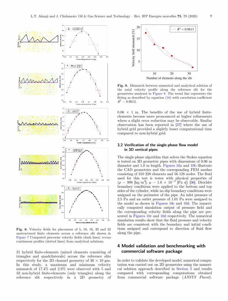
21 hybrid finite-elements (mixed elements consisting oftriangles and quadrilaterals) across the reference slitsrespectively for the 2D channel geometry of 30 � 10 lm.In this study, a maximum and minimum velocitymismatch of 17.4% and 2.9% were observed with 5 and32 non-hybrid finite-elements (only triangles) along thereference slit respectively in a 2D geometry of

0.06 � 1 m. The benefits of the use of hybrid finite-elements become more pronounced at higher refinementswhere a slight error reduction may be observable. Similarobservation has been reported in [37] where the use ofhybrid grid provided a slightly lesser computational timecompared to non-hybrid grid.

3.2 Verification of the single-phase flow modelin 3D vertical pipes

The single-phase algorithm that solves the Stokes equationis tested on 3D geometric pipes with dimensions of 0.06 mdiameter and 1.0 m length. Figures 10a and 10b illustratethe CAD geometries and the corresponding FEM meshesconsisting of 310 228 elements and 56 128 nodes. The fluidused for this test is water with physical properties of(q = 998 [kg/m3]; l = 1.0 � 10�3 [Pa s]) [36]. Dirichletboundary conditions were applied to the bottom and topsides of the cylinder, while no slip boundary conditions wereassigned on the perimeter of the pipe. An inlet pressure of2.5 Pa and an outlet pressure of 1.01 Pa were assigned tothe model as shown in Figures 10c and 10d. The numeri-cally computed simulation output of pressure field andthe corresponding velocity fields along the pipe are pre-sented in Figures 10c and 10d respectively. The numericalsimulation results show that the fluid pressure and velocityfields are consistent with the boundary and initial condi-tions assigned and correspond to direction of fluid flowalong the pipe.

4 Model validation and benchmarking withcommercial software package

In order to validate the developed model, numerical compu-tation was carried out on 2D geometries using the numeri-cal solution approach described in Section 2 and resultscompared with corresponding computations obtainedfrom commercial software package (ANSYS Fluent).

Fig. 8. Velocity fields for placement of 5, 10, 16, 20 and 32unstructured finite elements across a reference slit shown inFigure 7 Computed piecewise velocity fields (dash lines) versuscontinuous profiles (dotted lines) from analytical solutions.

Fig. 9. Mismatch between numerical and analytical solution ofthe axial velocity profile along the reference slit for thegeometries analysed in Figure 8. The trend line represents thefitting as described by equation (18) with correlation coefficientR2 = 0.9613.

L.T. Akanji and J. Chidamoio: Oil & Gas Science and Technology – Rev. IFP Energies nouvelles 75, 79 (2020) 9

Two comparisons with commercial simulator involving(i) computation of axial velocity field profiles along the pipelength and (ii) computation of parabolic velocity field

profiles at predefined reference slits along the pipe length,were carried out. Further, validation was conducted bycomparing computed results with experimentally measureddata. The laboratory measured data were obtained as partof a complementary investigation on flow in pipe researchproject (see Chidamoio [34]).

4.1 Benchmarking of CSMP++ simulation withANSYS Fluent simulations – axial velocity profiles

In this case, fluid pressure has been assigned as Dirichletboundaries at both the inlet and outlet sections of the pipe.The 2D model shown in Figure 6 is used for the purpose ofthis analysis. The model is a 0.06 m width and 1.0 m lengthpipe where the inlet is located at the bottom and the outletat the top. In ANSYS Fluent, a Dirichlet boundary condi-tion is applied by assigning n̂ �~v ¼ U 0 at the inlet whilethe outlet boundary is placed at the top of the tubing wherea Neumann pressure boundary condition is applied on theoutlet. The outlet pressure is set equal to one bar, meaningthat the outlet is open to the environment and the onlypressure acting at the outlet is atmospheric pressure [38].The outer surfaces of the tubing are treated as wall withno slip and no penetration ~u � t̂ ¼ 0;~u � n̂ ¼ 0, where t̂and n̂ denote the unit tangent on the boundary and unitnormal to the boundary respectively. Figures 11a and 11bshow the results of the velocity field computed fromANSYSFluent simulations and from this work respectively. Thetwo results are in very good agreement and within an aver-age relative error of 0.9%.

Fig. 10. (a) Cylindrical geometry model and (b) corresponding volume mesh consisting of 310 228 elements and 56 128 nodes.(c) Pressure profile along the 3D vertical pipe with the maximum test inlet pressure of 2.5 Pa and outlet pressure of 1.01 Pa.In-between the inlet and outlet pressure is a gradient that is consistent with imposed values and the physical geometry investigated.(d) Velocity profile along the 3D vertical pipe with the imposed no slip boundary conditions on the surface of the pipe and maximumvelocity profile at the middle of the pipe corresponding to the parabolic flow profile.

Fig. 11. Velocity profile for the numerical simulation obtainedfrom ANSYS Fluent package is shown in (a), while (b) shows theresult obtained from this numerical computation approach(CSMP++).

L.T. Akanji and J. Chidamoio: Oil & Gas Science and Technology – Rev. IFP Energies nouvelles 75, 79 (2020)10

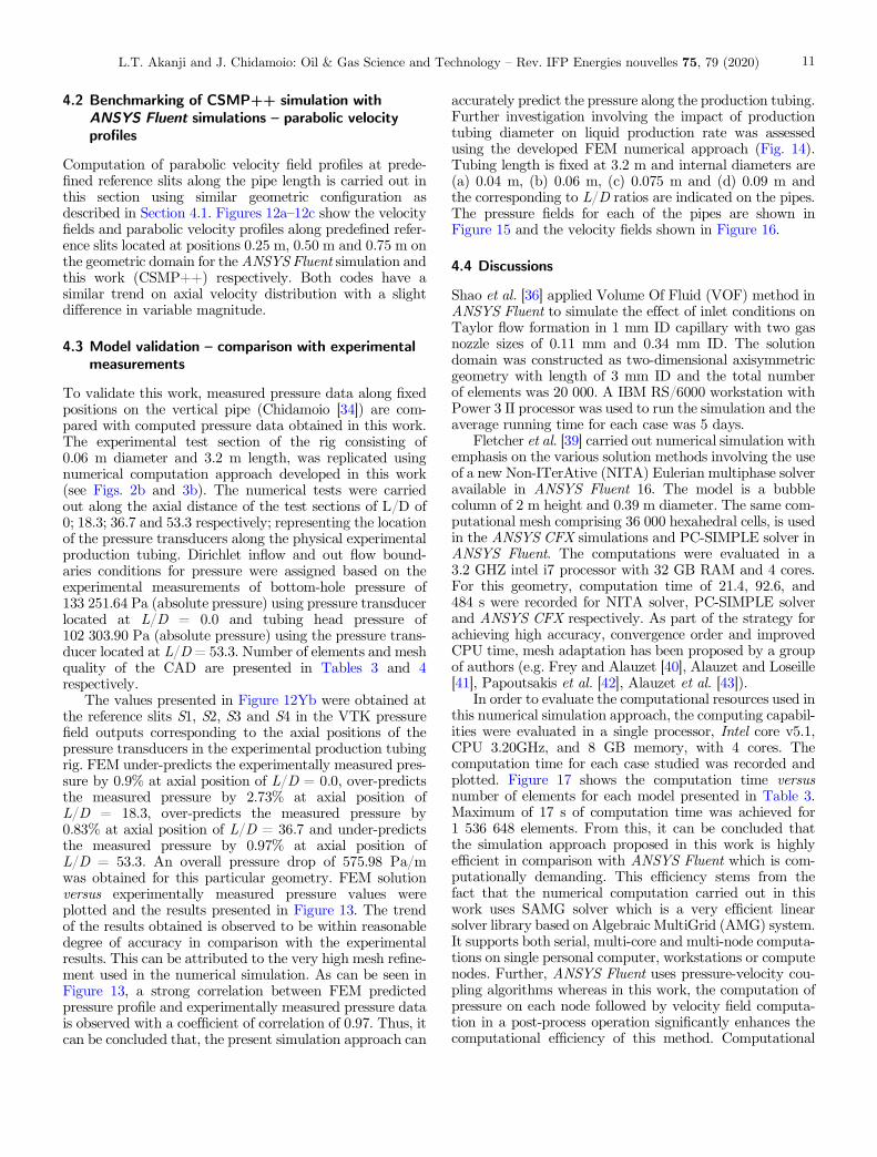
4.2 Benchmarking of CSMP++ simulation withANSYS Fluent simulations – parabolic velocityprofiles

Computation of parabolic velocity field profiles at prede-fined reference slits along the pipe length is carried out inthis section using similar geometric configuration asdescribed in Section 4.1. Figures 12a–12c show the velocityfields and parabolic velocity profiles along predefined refer-ence slits located at positions 0.25 m, 0.50 m and 0.75 m onthe geometric domain for the ANSYS Fluent simulation andthis work (CSMP++) respectively. Both codes have asimilar trend on axial velocity distribution with a slightdifference in variable magnitude.

4.3 Model validation – comparison with experimentalmeasurements

To validate this work, measured pressure data along fixedpositions on the vertical pipe (Chidamoio [34]) are com-pared with computed pressure data obtained in this work.The experimental test section of the rig consisting of0.06 m diameter and 3.2 m length, was replicated usingnumerical computation approach developed in this work(see Figs. 2b and 3b). The numerical tests were carriedout along the axial distance of the test sections of L/D of0; 18.3; 36.7 and 53.3 respectively; representing the locationof the pressure transducers along the physical experimentalproduction tubing. Dirichlet inflow and out flow bound-aries conditions for pressure were assigned based on theexperimental measurements of bottom-hole pressure of133 251.64 Pa (absolute pressure) using pressure transducerlocated at L/D = 0.0 and tubing head pressure of102 303.90 Pa (absolute pressure) using the pressure trans-ducer located at L/D = 53.3. Number of elements and meshquality of the CAD are presented in Tables 3 and 4respectively.

The values presented in Figure 12Yb were obtained atthe reference slits S1, S2, S3 and S4 in the VTK pressurefield outputs corresponding to the axial positions of thepressure transducers in the experimental production tubingrig. FEM under-predicts the experimentally measured pres-sure by 0.9% at axial position of L/D = 0.0, over-predictsthe measured pressure by 2.73% at axial position ofL/D = 18.3, over-predicts the measured pressure by0.83% at axial position of L/D = 36.7 and under-predictsthe measured pressure by 0.97% at axial position ofL/D = 53.3. An overall pressure drop of 575.98 Pa/mwas obtained for this particular geometry. FEM solutionversus experimentally measured pressure values wereplotted and the results presented in Figure 13. The trendof the results obtained is observed to be within reasonabledegree of accuracy in comparison with the experimentalresults. This can be attributed to the very high mesh refine-ment used in the numerical simulation. As can be seen inFigure 13, a strong correlation between FEM predictedpressure profile and experimentally measured pressure datais observed with a coefficient of correlation of 0.97. Thus, itcan be concluded that, the present simulation approach can

accurately predict the pressure along the production tubing.Further investigation involving the impact of productiontubing diameter on liquid production rate was assessedusing the developed FEM numerical approach (Fig. 14).Tubing length is fixed at 3.2 m and internal diameters are(a) 0.04 m, (b) 0.06 m, (c) 0.075 m and (d) 0.09 m andthe corresponding to L/D ratios are indicated on the pipes.The pressure fields for each of the pipes are shown inFigure 15 and the velocity fields shown in Figure 16.

4.4 Discussions

Shao et al. [36] applied Volume Of Fluid (VOF) method inANSYS Fluent to simulate the effect of inlet conditions onTaylor flow formation in 1 mm ID capillary with two gasnozzle sizes of 0.11 mm and 0.34 mm ID. The solutiondomain was constructed as two-dimensional axisymmetricgeometry with length of 3 mm ID and the total numberof elements was 20 000. A IBM RS/6000 workstation withPower 3 II processor was used to run the simulation and theaverage running time for each case was 5 days.

Fletcher et al. [39] carried out numerical simulation withemphasis on the various solution methods involving the useof a new Non-ITerAtive (NITA) Eulerian multiphase solveravailable in ANSYS Fluent 16. The model is a bubblecolumn of 2 m height and 0.39 m diameter. The same com-putational mesh comprising 36 000 hexahedral cells, is usedin the ANSYS CFX simulations and PC-SIMPLE solver inANSYS Fluent. The computations were evaluated in a3.2 GHZ intel i7 processor with 32 GB RAM and 4 cores.For this geometry, computation time of 21.4, 92.6, and484 s were recorded for NITA solver, PC-SIMPLE solverand ANSYS CFX respectively. As part of the strategy forachieving high accuracy, convergence order and improvedCPU time, mesh adaptation has been proposed by a groupof authors (e.g. Frey and Alauzet [40], Alauzet and Loseille[41], Papoutsakis et al. [42], Alauzet et al. [43]).

In order to evaluate the computational resources used inthis numerical simulation approach, the computing capabil-ities were evaluated in a single processor, Intel core v5.1,CPU 3.20GHz, and 8 GB memory, with 4 cores. Thecomputation time for each case studied was recorded andplotted. Figure 17 shows the computation time versusnumber of elements for each model presented in Table 3.Maximum of 17 s of computation time was achieved for1 536 648 elements. From this, it can be concluded thatthe simulation approach proposed in this work is highlyefficient in comparison with ANSYS Fluent which is com-putationally demanding. This efficiency stems from thefact that the numerical computation carried out in thiswork uses SAMG solver which is a very efficient linearsolver library based on Algebraic MultiGrid (AMG) system.It supports both serial, multi-core and multi-node computa-tions on single personal computer, workstations or computenodes. Further, ANSYS Fluent uses pressure-velocity cou-pling algorithms whereas in this work, the computation ofpressure on each node followed by velocity field computa-tion in a post-process operation significantly enhances thecomputational efficiency of this method. Computational

L.T. Akanji and J. Chidamoio: Oil & Gas Science and Technology – Rev. IFP Energies nouvelles 75, 79 (2020) 11

Fig. 12. Axial velocity distribution along the geometric domain for (a) ANSYS Fluent simulation and (b) CSMP++ simulation. Inboth cases, (c1)–(c3) represent the axial velocity profile at positions 0.25 m, 0.5 m and 0.75 m along the production tubing.

Fig. 13. FEM predicted and experimentally measured pressureat 4 measurement points S1, S2, S3 and S4 along the productiontubing.

Fig. 14. Experimentally measured versus FEM predicted (M/P)pressure at 4 points S1, S2, S3 and S4 along the productiontubing.

Fig. 15. Pressure field along vertical production tubing. Modelheight is fixed at 3.2 m but inner diameters D are: (a) 0.04 m, (b)0.06 m, (c) 0.075 m and (d) 0.09 m respectively. In each of (a–d)the referenced positions along the pipe correspond to thelocation of the actual pressure sensors (S1, S2, S3, S4) placedon the physical experimental rig. The length-to-diameter L/Dratios along the pipes are as indicated on the geometric models.

L.T. Akanji and J. Chidamoio: Oil & Gas Science and Technology – Rev. IFP Energies nouvelles 75, 79 (2020)12

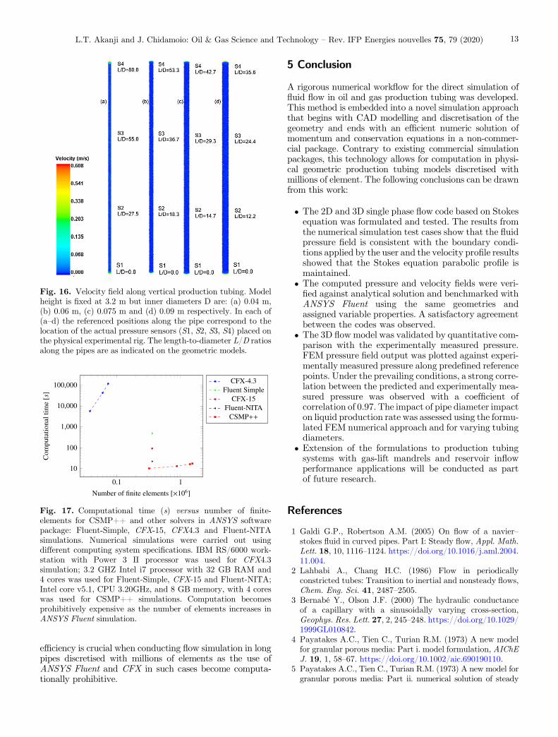
efficiency is crucial when conducting flow simulation in longpipes discretised with millions of elements as the use ofANSYS Fluent and CFX in such cases become computa-tionally prohibitive.

5 Conclusion

A rigorous numerical workflow for the direct simulation offluid flow in oil and gas production tubing was developed.This method is embedded into a novel simulation approachthat begins with CAD modelling and discretisation of thegeometry and ends with an efficient numeric solution ofmomentum and conservation equations in a non-commer-cial package. Contrary to existing commercial simulationpackages, this technology allows for computation in physi-cal geometric production tubing models discretised withmillions of element. The following conclusions can be drawnfrom this work:

� The 2D and 3D single phase flow code based on Stokesequation was formulated and tested. The results fromthe numerical simulation test cases show that the fluidpressure field is consistent with the boundary condi-tions applied by the user and the velocity profile resultsshowed that the Stokes equation parabolic profile ismaintained.

� The computed pressure and velocity fields were veri-fied against analytical solution and benchmarked withANSYS Fluent using the same geometries andassigned variable properties. A satisfactory agreementbetween the codes was observed.

� The 3D flow model was validated by quantitative com-parison with the experimentally measured pressure.FEM pressure field output was plotted against experi-mentally measured pressure along predefined referencepoints. Under the prevailing conditions, a strong corre-lation between the predicted and experimentally mea-sured pressure was observed with a coefficient ofcorrelation of 0.97. The impact of pipe diameter impacton liquid production rate was assessed using the formu-lated FEM numerical approach and for varying tubingdiameters.

� Extension of the formulations to production tubingsystems with gas-lift mandrels and reservoir inflowperformance applications will be conducted as partof future research.

References

1 Galdi G.P., Robertson A.M. (2005) On flow of a navier–stokes fluid in curved pipes. Part I: Steady flow, Appl. Math.Lett. 18, 10, 1116–1124. https://doi.org/10.1016/j.aml.2004.11.004.

2 Lahbabi A., Chang H.C. (1986) Flow in periodicallyconstricted tubes: Transition to inertial and nonsteady flows,Chem. Eng. Sci. 41, 2487–2505.

3 Bernabé Y., Olson J.F. (2000) The hydraulic conductanceof a capillary with a sinusoidally varying cross-section,Geophys. Res. Lett. 27, 2, 245–248. https://doi.org/10.1029/1999GL010842.

4 Payatakes A.C., Tien C., Turian R.M. (1973) A new modelfor granular porous media: Part i. model formulation, AIChEJ. 19, 1, 58–67. https://doi.org/10.1002/aic.690190110.

5 Payatakes A.C., Tien C., Turian R.M. (1973) A new model forgranular porous media: Part ii. numerical solution of steady

Fig. 16. Velocity field along vertical production tubing. Modelheight is fixed at 3.2 m but inner diameters D are: (a) 0.04 m,(b) 0.06 m, (c) 0.075 m and (d) 0.09 m respectively. In each of(a–d) the referenced positions along the pipe correspond to thelocation of the actual pressure sensors (S1, S2, S3, S4) placed onthe physical experimental rig. The length-to-diameter L/D ratiosalong the pipes are as indicated on the geometric models.

Fig. 17. Computational time (s) versus number of finite-elements for CSMP++ and other solvers in ANSYS softwarepackage: Fluent-Simple, CFX-15, CFX4.3 and Fluent-NITAsimulations. Numerical simulations were carried out usingdifferent computing system specifications. IBM RS/6000 work-station with Power 3 II processor was used for CFX4.3simulation; 3.2 GHZ Intel i7 processor with 32 GB RAM and4 cores was used for Fluent-Simple, CFX-15 and Fluent-NITA;Intel core v5.1, CPU 3.20GHz, and 8 GB memory, with 4 coreswas used for CSMP++ simulations. Computation becomesprohibitively expensive as the number of elements increases inANSYS Fluent simulation.

L.T. Akanji and J. Chidamoio: Oil & Gas Science and Technology – Rev. IFP Energies nouvelles 75, 79 (2020) 13

state incompressible newtonian flow through periodicallyconstricted tubes, AIChE J. 19, 1, 67–76. https://doi.org/10.1002/aic.690190111.

6 Koplik J. (1982) Creeping flow in two-dimensional networks,J. Fluid Mech. 119, 219–247. https://doi.org/10.1017/S0022112082001323.

7 Chidamoio J., Akanji L., Rafati R. (2017) Prediction ofoptimum length to diameter ratio for two-phase fluid flowdevelopment in vertical pipes, Adv. Pet. Explor. Develop. 14,1, 1–17.

8 Hernandez A. (2016) Fundamentals of gas lift engineering:Well design and troubleshooting, Elsevier.

9 Al-Atabi M., Al-Zuhair S., Chin S.B., Luo X.Y. (2006)Pressure drop in laminar and turbulent flows in circular pipewith baffles – an experimental and analytical study, Int. J.Fluid Mech. Res. 33, 4, 303–319. https://doi.org/10.1615/InterJFluidMechRes.v33.i4.10.

10 Al-Atabi M., Al-Zuhair S., Chin S.B., Luo X.Y. (2010) Flowof non-newtonian fluids in porous media, J. Polym. Sci. 48,23, 2437–2467.

11 Sochi T. (2015) Flow of navier-stokes fluids in cylindricalelastic tubes, J. Appl. Fluid Mech. 8, 2, 181–188.

12 Sabooniha E., Rokhforouz M.R., Ayatollahi S. (2019) Pore-scale investigation of selective plugging mechanism inimmiscible two-phase flow using phase-field method, OilGas Sci. Technol. - Rev. IFP Energies nouvelles 74, 78.10.2516/ogst/2019050.

13 Sisavath S., Jing X., Zimmerman R.W. (2001) Creeping flowthrough a pipe of varying radius, Phys. Fluids 13, 10, 2762–2772. https://doi.org/10.1063/1.1399289.

14 Tilton J.N., Payatakes A.C. (1984) Collocation solution ofcreeping newtonian flow through sinusoidal tubes: A correc-tion, AIChE J. 30, 6, 1016–1021. https://doi.org/10.1002/aic.690300628.

15 Deiber J.A., Schowalter W.R. (1979) Flow through tubeswith sinusoidal axial variations in diameter, AIChE J. 25, 4,638–645. https://doi.org/10.1002/aic.690250410.

16 Hemmat M., Borhan A. (1995) Creeping flow throughsinusoidally constricted capillaries, Phys. Fluids 7, 9, 2111–2121. https://doi.org/10.1063/1.868462.

17 Sirisup S., Karniadakis G.E., Saelim N., Rockwell D. (2004)Dns and experiments of flow past a wired cylinder at lowreynolds number, Eur. J. Mech. – B/Fluids 23, 1, 181–188.https://doi.org/10.1016/j.euromechflu.2003.04.003.

18 Ge M., Xu C. (2010) Direct numerical simulation of flow inchannel with time-dependent wall geometry, Appl. Math.Mech. 31, 1, 97–108. https://doi.org/10.1007/s10483-010-0110-x.

19 Ould-Rouiss M., Redjem-Saad L., Lauriat G. (2009) Directnumerical simulation of turbulent heat transfer in annuli:Effect of heat flux ratio, Int. J. Heat Fluid Flow 30, 4, 579–589. https://doi.org/10.1016/j.ijheatfluidflow.2009.02.018.

20 Tamano S., Itoh M., Hoshizaki K., Yokota K. (2007)Direct numerical simulation of the drag-reducing turbulentboundary layer of viscoelastic fluid, Phys. Fluids 19, 7,75–106. doi:https://doi.org/10.1063/1.2749816.

21 Zhu Z., Yang H., Chen T. (2009) Direct numerical simulationof turbulent flow in a straight square duct at reynoldsnumber 600, J. Hydrodyn. Ser. B 21, 5, 600–607. https://doi.org/10.1016/S1001-6058(08)60190-0.

22 Li D., Fan J., Luo K., Cen K. (2011) Direct numericalsimulation of a particle-laden low reynolds number turbulent

round jet, Int. J. Multiph. Flow 37, 6, 539–554. https://doi.org/10.1016/j.ijmultiphaseflow.2011.03.013.

23 Li B., Liu N., Lu X. (2006) Direct numerical simulation ofwall-normal rotating turbulent channel flow with heattransfer, Int. J. Heat Mass Trans. 49, 5, 1162–1175.https://doi.org/10.1016/j.ijheatmasstransfer.2005.08.030.

24 Stüben K. (2001) A review of algebraic multigrid, J. Comput.Appl. Math. 128, 1, 281–309. https://doi.org/10.1016/S0377-0427(00)00516-1. ID: 271610.

25 Guet S., Ooms G., Oliemans R.V.A., Mudde R.F. (2003)Bubble injector effect on the gaslift efficiency, AIChE J. 49,9, 2242–2252.

26 Batchelor G.K. (1967) An introduction to fluid dynamics,Cambridge University Press.

27 Akanji L.T., Matthai S.K. (2010) Finite element-basedcharacterization of pore-scale geometry and its impact onfluid flow, Transp. Porous Media 81, 2, 241–259. https://doi.org/10.1007/s11242-009-9400-7.

28 Babuvška I., Rheinboldt W.C. (1978) Error estimates foradaptive finite element computations, SIAM J. Numer. Anal.15, 4, 736–754. https://doi.org/10.1137/071504.

29 Smith I.M., Griffiths D.V., Margetts L. (2013) Programmingthe finite element method, John Wiley & Sons.

30 Matthäi S.K., Geiger S., Roberts S.G. (2001) ComplexSystems Platform: CSP3D3.0 user’s guide, ETH ZurichResearch Collection.

31 Matthai S.K., Roberts S.G. (1996) The influence of faultpermeability on single-phase fluid flow near fault-sandintersections: Results from steady-state high-resolutionmodels of pressure-driven fluid flow, Assoc. Pet. Geol. Bull.80, 11, 1763–1779.

32 Garcia X., Akanji L.T., Blunt M.J., Matthai S.K., LathamJ.P. (2009) Numerical study of the effects of particle shapeand polydispersity on permeability, Phys. Rev. E 80, 021304.https://doi.org/10.1103/PhysRevE.80.021304.

33 Akanji L.T., Nasr G., Matthai S.K. (2013) Estimation ofhydraulic anisotropy of unconsolidated granular packs usingfinite element methods, Int. J. Multiphys. 7, 2, 153–166.

34 Chidamoio J.F. (2018) Experimental and numerical mod-elling of gaslift cavitation and instabilities in oil producingwells, PhD Thesis, Petroleum Engineering Division, Univer-sity of Aberdeen.

35 Anderson A.E., Ellis B.J., Weiss J.A. (2007) Verification,validation and sensitivity studies in computational biomechan-ics, Comput. Meth. Biomech. Biomed. Eng. 10, 3, 171–184.

36 Shao N., Salman W., Gavriilidis A., Angeli P. (2008) Cfdsimulations of the effect of inlet conditions on taylor flowformation, Int. J. Heat Fluid Flow 296, 1603–1611.

37 Kroll N., Gerhold Th., Melber S., Heinrich R., Schwarz Th.,Schöning B. (2002) Parallel large scale computations foraerodynamic aircraft design with the German CFD systemmegaflow, in Wilders P., Ecer A., Satofuka N., Periaux J.,Fox P. (eds), Parallel Computational Fluid Dynamics 2001,North-Holland, Amsterdam, pp. 227–236. https://doi.org/10.1016/B978-044450672-6/50080-3.

38 Inc ANSYS (2013) ANSYS FLUENT 12.0 user’s guide,ANSYS, Canonsburg, Pennsylvania, United States.

39 Fletcher D.F., McClure D.D., Kavanagh J.M., Barton G.W.(2017) Cfd simulation of industrial bubble columns: Numer-ical challenges and model validation successes, Appl. Math.Model. 44, 25–42. https://doi.org/10.1016/j.apm.2016.08.033.

L.T. Akanji and J. Chidamoio: Oil & Gas Science and Technology – Rev. IFP Energies nouvelles 75, 79 (2020)14

40 Frey P.-J., Alauzet F. (2005) Anisotropic mesh adaptationfor cfd computations, Comput. Meth. Appl. Mech. Eng. 194,48–49, 5068–5082.

41 Alauzet F., Loseille A. (2016) A decade of progress onanisotropic mesh adaptation for computational fluid dynamics,Comput.-Aid. Design 72, 13–39. https://doi.org/10.1016/j.cad.2015. 09.005.

42 Papoutsakis A., Sazhin S.S., Begg S., Danaila I., Luddens F.(2018) An efficient adaptive mesh refinement (amr) algorithm

for the discontinuous galerkin method: Applications for thecomputation of compressible two-phase flows, J. Comput.Phys. 363, 399–427. https://doi.org/10.1016/j.jcp.2018.02.048.

43 Alauzet F., Loseille A., Olivier G. (2018) Time-accuratemulti-scale anisotropic mesh adaptation for unsteady flows inCFD, J. Comput. Phys. 373, 28–63. https://doi.org/10.1016/j.jcp.2018.06.043.

L.T. Akanji and J. Chidamoio: Oil & Gas Science and Technology – Rev. IFP Energies nouvelles 75, 79 (2020) 15