a first-principles approach to protein–ligand interaction ... related to ligand binding, drug...
TRANSCRIPT
LUND UNIVERSITY
PO Box 117221 00 Lund+46 46-222 00 00
A first-principles approach to protein–ligand interaction
Söderhjelm, Pär
Published: 2009-01-01
Link to publication
Citation for published version (APA):Söderhjelm, P. (2009). A first-principles approach to protein–ligand interaction Department of TheoreticalChemistry, Lund University
General rightsCopyright and moral rights for the publications made accessible in the public portal are retained by the authorsand/or other copyright owners and it is a condition of accessing publications that users recognise and abide by thelegal requirements associated with these rights.
• Users may download and print one copy of any publication from the public portal for the purpose of privatestudy or research. • You may not further distribute the material or use it for any profit-making activity or commercial gain • You may freely distribute the URL identifying the publication in the public portalTake down policyIf you believe that this document breaches copyright please contact us providing details, and we will removeaccess to the work immediately and investigate your claim.

Download date: 23. Jun. 2018

A first-principles approach toprotein–ligand interaction
Thesis submitted for the degree of
Doctor of Philosophy by
Pär Söderhjelm
Department of Theoretical Chemistry
AKADEMISK AVHANDLING för avläggande av filosofie doktorsexamen vid
naturvetenskapliga fakulteten, Lunds Universitet, kommer att offentligen försvaras
i
Hörsal B, Kemicentrum, fredagen den 6 Februari 2009, kl 10.15
Fakultetens opponent är
Dr. Jean-Philip Piquemal
Laboratoire de Chimie Théorique, Université Pierre et Marie Curie, Paris, Frankrike

c© Pär Söderhjelm, 2009
Lund University, SwedenDoctoral dissertation in Theoretical Chemistry
ISBN 978-91-628-7665-4
Printed by Media Tryck, Lund

Contents
Preface v
Populärvetenskaplig sammanfattning vii
List of papers xi
Acknowledgements xiii
1 Chemistry from a theoretical perspective 11.1 The electronic problem: Quantum chemistry . . . . . . . . . . . 2
1.1.1 The basis set problem . . . . . . . . . . . . . . . . . . . . 41.1.2 The electron-correlation problem . . . . . . . . . . . . . . 5
1.2 The nuclear problem: Statistical mechanics . . . . . . . . . . . . 71.2.1 Physical description . . . . . . . . . . . . . . . . . . . . . 71.2.2 Computation . . . . . . . . . . . . . . . . . . . . . . . . . 9
2 Intermolecular interactions 112.1 The supermolecular approach . . . . . . . . . . . . . . . . . . . . 11
2.1.1 Electron correlation . . . . . . . . . . . . . . . . . . . . . 112.1.2 Basis set . . . . . . . . . . . . . . . . . . . . . . . . . . . . 13
2.2 Perturbative approach . . . . . . . . . . . . . . . . . . . . . . . . 142.2.1 Qualitative picture . . . . . . . . . . . . . . . . . . . . . . 152.2.2 Quantum-chemical perturbation theory . . . . . . . . . . 162.2.3 Molecular mechanics . . . . . . . . . . . . . . . . . . . . . 19
2.3 Molecular mechanics based on quantum chemistry . . . . . . . . 202.3.1 Electrostatic interaction energy . . . . . . . . . . . . . . . 212.3.2 Polarization . . . . . . . . . . . . . . . . . . . . . . . . . . 222.3.3 Dispersion . . . . . . . . . . . . . . . . . . . . . . . . . . . 292.3.4 Repulsion . . . . . . . . . . . . . . . . . . . . . . . . . . . 302.3.5 Charge transfer . . . . . . . . . . . . . . . . . . . . . . . . 34
iii

iv CONTENTS
3 Protein–ligand affinities 353.1 Theory . . . . . . . . . . . . . . . . . . . . . . . . . . . . . . . . . 363.2 Path-based methods . . . . . . . . . . . . . . . . . . . . . . . . . 37
3.2.1 Relative affinities . . . . . . . . . . . . . . . . . . . . . . . 373.2.2 Absolute affinities . . . . . . . . . . . . . . . . . . . . . . 373.2.3 Potential of mean force . . . . . . . . . . . . . . . . . . . 38
3.3 End-point methods . . . . . . . . . . . . . . . . . . . . . . . . . . 393.3.1 Perturbations from single simulations . . . . . . . . . . . 393.3.2 Linear interaction energy (LIE) . . . . . . . . . . . . . . . 403.3.3 MM/PBSA . . . . . . . . . . . . . . . . . . . . . . . . . . 40
3.4 Solvation . . . . . . . . . . . . . . . . . . . . . . . . . . . . . . . 423.4.1 Polar solvation . . . . . . . . . . . . . . . . . . . . . . . . 433.4.2 Non-polar solvation . . . . . . . . . . . . . . . . . . . . . 44
3.5 Potential energy . . . . . . . . . . . . . . . . . . . . . . . . . . . 44
4 Summary of the papers 474.1 Paper I: Exchange-repulsion energy . . . . . . . . . . . . . . . . . 474.2 Paper II: Multipoles and polarizabilities . . . . . . . . . . . . . . 484.3 Papers III and IV: Polarization models . . . . . . . . . . . . . . . 49
4.3.1 Densities . . . . . . . . . . . . . . . . . . . . . . . . . . . 494.3.2 Energies . . . . . . . . . . . . . . . . . . . . . . . . . . . . 51
4.4 Paper V, VI, and VII: The PMISP method . . . . . . . . . . . . 524.4.1 Methods . . . . . . . . . . . . . . . . . . . . . . . . . . . . 534.4.2 Results . . . . . . . . . . . . . . . . . . . . . . . . . . . . 53
4.5 Conclusions and outlook . . . . . . . . . . . . . . . . . . . . . . . 55
Bibliography 57

Preface
When the subject of force fields for protein simulations was reviewed some yearsago by Ponder and Case [1], the authors noted that “without further researchinto the accuracy of force-field potentials, future macromolecular modeling maywell be limited more by validity of the energy functions, particularly electrostaticterms, than by technical ability to perform the computations. For many calcu-lations related to ligand binding, drug design, and protein structure prediction,accuracy of the underlying potential functions is critical.”
The current work is my contribution to this problem. The thesis describessome basic attempts to get a grip of how accurate force fields are, how accuratethey can become, and where to put in the effort to improve them, all in thecontext of using them for predicting interaction energies in biological systems.
The physical laws underlying chemistry have been known for about 80 years [2].What prevents us from calculating e.g. protein–ligand affinities directly fromthese laws, i.e. from first principles, is essentially that they lead to equationsthat cannot be solved exactly. Therefore, this thesis explores an approach, inwhich the intermolecular potentials are purely based on quantum chemistry,but approximated in several ways. In principle, the accuracy of each approx-imation can be thoroughly tested, so that the quantum-chemical value can beapproached. In contrast, most approaches to binding affinities are empirical,using experimental data on at least some level. A drawback of such approachesare that they are not systematically improvable.
The structure of the thesis is as follows. The first chapter introduces theconstitution of matter as it appears to a computational chemist like me. Thesecond chapter deals with calculating interaction energies, focusing on how touse quantum chemistry to derive simpler methods that can be used for largersystems. The third chapter addresses the protein–ligand binding problem, whichin addition to interaction energies encompasses several difficult problems, suchas sampling and solvation. The fourth chapter gives a summary of the papersincluded in the thesis and the conclusions I have drawn from them. The papersare attached at the end of the thesis.
The purpose of the first three chapters is to give an overview of the theoryand computational approaches that underlie my own work. My goal has beento present a non-mathematical description, giving a personal (and far from
v

vi Chapter 0: Preface
exhaustive) selection of references that can provide details to the interestedreader. There are indeed many formulas, but that does not mean you haveto understand them to read the thesis. They are there simply because I likeformulas. Knowing that there is a formula and seeing what quantities are in itis a great comfort to me, even if I do not have a clue how to evaluate it.
Lund, December 2008
Pär Söderhjelm

Populärvetenskaplig
sammanfattning
Många biologiska processer på molekylär nivå börjar med att två molekylerbinder till varandra på ett speciellt sätt. Exempelvis måste ett enzym, d.v.s.ett protein som är designat för att utföra en viss kemisk reaktion, binda tilljust den molekylen som ska reagera. Ett annat exempel är vårt luktsinne, därdoftämnet måste binda till en receptor, som också är ett protein, för att utlösaen nervsignal till hjärnan. Den mindre molekylen som binder till proteinet kallasofta ligand.
Denna bindingsprocess brukar kallas molekylär igenkänning, men har natur-ligtvis ingenting med en intelligent process att göra. Molekylerna följer en banasom bestäms av fysikens lagar där de flyter runt i en trög soppa av vatten-molekyler, joner och andra små och stora molekyler. På sin väg innan de träffar“den rätte” hinner de stöta ihop med tusentals andra tänkbara partners, men ombindningsstyrkan är för liten fastnar de inte alls eller bara kanske en kort stund.Om bindningsstyrkan däremot är stor sitter molekylerna ihop länge. Den häravhandlingen handlar om att teoretiskt beräkna bindningsstyrkan mellan ettprotein och en annan molekyl.
sådana beräkningar är bl.a. av stort intresse för läkemedelsindustrin. Omman kan hitta en molekyl som binder starkare till ett enzym än den naturligamolekyl som enzymet egentligen ska binda till, så kommer den att blockeraenzymet så att den naurliga molekylen inte får plats och ingen reaktion kan ske,vilket ibland kan vara ett sätt att behandla en sjukdom. Förutsättningen föratt en sådan molekyl ska fungera som läkemedel är förstås också att man lyckasfå in den i cellen och att den inte binder till andra proteiner och på så vis ställertill oreda.
Trots att proteiner är jättestora för att vara molekyler är de små med våramått mätt, bara några nanometer (milliondels millimeter). Vi kan därför inteens med mikroskop se hur det ser ut när en ligand binder till ett protein. Meddatorns hjälp kan vi däremot göra oss en konstgjord bild av det hela (Fig. 1).Datorn är också det redskap vi behöver för att uppskatta bindningsstyrkan.
Som en första approximation brukar man kunna anta att för att ligandenska binda starkt, så ska den “passa in” i proteinet, som en nyckel i ett lås.
vii

viii Chapter 0: Populärvetenskaplig sammanfattning
Figure 1: En ögonblicksbild av ett protein (avidin) som bundit in en ligand (biotin),färgad lila på bilden. Proteinets atomer har förminskats för att man ska se ligandensom egentliger ligger helt inbäddad. Varje färg motsvarar en sorts atom: vit=väte,röd=syre, ljusblå=kol, blå=kväve och gul=svavel. Allt tomrum är i verkligheten fylltav vattenmolekyler.

ix
Ligandens yta ska alltså vara som en avgjutning av proteinets yta, så att de kanligga intill varandra utan att det blir några hål. Detta beror på att de flestasorters molekyler attraherar varandra när man kommer tillräckligt nära. Det ärt.ex. sådana krafter som gör att en ödla kan gå uppför en lodrät vägg.
För att få någorlunda bra resultat krävs mer noggranna beräkningsmodellersom också tar hänsyn till den kemiska strukturen på både proteinet och liganden.Det räcker alltså inte att ytorna ligger intill varandra, det måste också varaytor som passar ihop, t.ex. en positivt och en negativt laddad yta. Detta kanbeskrivas med hjälp av ett kraftfält.
Ett kraftfält kan ses som en topografisk karta över t.ex. ett bergslandskap.Det talar om hur fördelaktigt det är för varje par av atomer att befinna signära varandra, eller rättare sagt hur energin varierar beroende på avståndetmellan dem. Enligt en grundläggande fysikalisk princip strävar systemet efteratt ha så låg energi som möjligt, d.v.s. komma så långt ner i dalgångarna sommöjligt. Atomerna är dock aldrig stilla utan kan snarare betraktas som ett gängdagisbarn som när de springer ner för backarna får sådan fart att de fortsätteruppför nästa backe med oförtröttlig energi. Denna dynamik måste man normaltockså ta hänsyn till i sina beräkningar. Endast om man kyler ner alltihop tillabsoluta nollpunkten (−273C) börjar atomerna lugna ner sig.
Den rätta kartan, den som motsvarar verkligheten, är tyvärr omöjlig attfinna eftersom vi inte kan se hur atomerna rör sig. Normalt nöjer man sigmed en karta som ger hyfsade resultat i genomsnitt. Detta är bekvämt, för närresultatet blir fel kan man alltid skylla på att kartan var dålig just där.
Det finns dock en annan utgångspunkt, och det är det som denna avhan-dling handlar om. Om vi tränger under skinnet på atomerna så ser vi att deegentligen består av en positivt laddad kärna samt ett antal negativa elektronersom snurrar runt kärnan. Vidare är elektronerna inte tvungna att stanna runt“sin” kärna utan snurrar fritt runt alla kärnor i molekylen och till och med mel-lan molekylerna. Lyckligtvis finns det en fysikalisk teori, kvantmekaniken, sombeskriver hur elektronerna fördelar sig och hur molekylerna därmed växelverkarmed varandra. Vi kan alltså räkna ut hur kartan ser ut!
Tyvärr är kvantmekanik praktiskt tillämpbar endast på små molekyler. Atträkna ut energin noggrant i en punkt på vår protein–ligand-karta skulle ta fleramiljarder år med dagens datorer. Och en miljondels miljondels sekund senarehar alla dagisbarnen flyttat sig och man får räkna om alltihop igen.
En lösning på detta är att i huvudsak använda den förenklade bilden medatomer, men att utnyttja den komplicerade bilden med elektroner för att för-bättra kartan lite i taget. Olika varianter på detta tema behandlas i de olikaartiklarna i denna avhandling. Exempelvis handlar den första artikeln om hurrepulsionen mellan molekylerna kan uppskattas utifrån hur mycket elektronernatillhörande vardera molekylen överlappar med varandra, medan den andra hand-lar om hur noggrant man kan uppskatta den elektriska växelverkan mellan t.ex.positiva och negativa molekylytor med hjälp av noggranna räkningar på varderaytan. De sista artiklarna handlar om hur man kan använda den komplicerade

x Chapter 0: Populärvetenskaplig sammanfattning
bilden för att räkna ut växelverkan mellan liganden och små bitar av proteinet,en i taget, medan effekter som beror på hela proteinet beräknas med den enklabilden.
Resultatet av dessa ansträngningar skulle kunna bli ett kraftfält för protein–ligand-interaktionsenergier som är helt byggt på fysikaliska principer (first prin-ciples), därav titeln på denna avhandling. Tyvärr är vi inte där ännu, men minförhoppning är att dessa små steg kan hjälpa till att så småningom uppnå dettamål.

List of papers
I. Comparison of overlap-based models for approximating the exchange-repulsion energyP. Söderhjelm, G. Karlström, and U. Ryde,Journal of Chemical Physics, 104, 244101 (2006)
II. Accuracy of distributed multipoles and polarizabilities: Com-parison between the LoProp and MpProp modelsP. Söderhjelm, J. W. Krogh, G. Karlström, U. Ryde, and R. Lindh,Journal of Computational Chemistry, 28, 1083 (2007)
III. Accuracy of typical approximations in classical models of inter-molecular polarizationP. Söderhjelm, A. Öhrn, U. Ryde, and G. Karlström,Journal of Chemical Physics, 128, 014102 (2008)
IV. On the coupling of intermolecular polarization and repulsionthrough pseudo-potentialsP. Söderhjelm and A. Öhrn,Chemical Physics Letters, DOI:10.1016/j.cplett.2008.11.074 (2008)
V. How accurate may a force field become? - A polarizable mul-tipole model combined with fragment-wise quantum-mechanicalcalculationsP. Söderhjelm and U. Ryde,Journal of Physical Chemistry A, in press
VI. Calculation of protein–ligand interaction energies by a fragmen-tation approach combining high-level quantum chemistry withclassical many-body effectsP. Söderhjelm, F. Aquilante, and U. Ryde,Submitted to Journal of Physical Chemistry B
VII. Ligand affinities estimated by quantum chemical calculationsP. Söderhjelm, J. Kongsted, and U. Ryde,Manuscript
xi

xii Chapter 0: List of papers
Other papers, not included in the thesis.
• Ligand affinities predicted with the MM/PBSA method: depen-dence on the simulation method and the force fieldA. Weis, K. Katebzadeh, P. Söderhjelm, I. Nilsson, and U. Ryde,Journal of Medicinal Chemistry, 49, 6596 (2006)
• Conformational dependence of charges in protein simulationsP. Söderhjelm and U. Ryde,Journal of Computational Chemistry, DOI: 10.1002/jcc.21097
• Proton transfer at metal sites in proteins studied by quantummechanical free-energy perturbationsM. Kaukonen, P. Söderhjelm, J. Heimdal, and U. Ryde,Journal of Chemical Theory and Computation, 4, 985 (2008)
• A QM/MM-PBSA method to estimate free energies for reac-tions in proteinsM. Kaukonen, P. Söderhjelm, J. Heimdal, and U. Ryde,Journal of Physical Chemistry B , 112, 12537 (2008)
• On the performance of quantum chemical methods to predictsolvatochromic effects. The case of acrolein in aqueous solutionK. Aidas, A. Mogelhoj, E. Nilsson, M. S. Johnson, K. V. Mikkelsen, O.Christiansen, P. Söderhjelm, and J. Kongsted,Journal of Chemical Physics, 128, 194503 (2008)
• Protein influence on electronic spectra modelled by multipolesand polarisabilitiesP. Söderhjelm, C. Husberg, A. Strambi, M. Olivucci, and U. Ryde,Journal of Chemical Theory and Computation, in press
• The ozone ring closure as a test for multi-state multi-configurationalsecond order perturbation theory (MS-CASPT2)L. De Vico, L. Pegado, J. Heimdal, P. Söderhjelm, and B. O. Roos,Chemical Physics Letters, 461, 136 (2008)
• Combined computational and crystallographic study of the oxi-dised states of [NiFe] hydrogenaseP. Söderhjelm and U. Ryde,Journal of Molecular Structure: THEOCHEM, 770, 199 (2006)
• How accurate are really continuum solvation models for drug-like molecules?J. Kongsted, P. Söderhjelm, and U. Ryde,Submitted to Journal of Chemical Theory and Computation
Acknowledgements
Först vill jag tacka Ulf för ditt varma ledarskap. Din dörr har alltid varit öppen,både bildligt och bokstavligt, och inget har varit för smått eller stort för att taupp med dig. När jag drivit iväg åt mitt håll har du inte hållit mig tillbaka, utantvärtom själv följt efter för att kunna vara det stöd som jag själv inte alltid harförstått att jag behövt. Du representerar även en nästan ofattbar effektivitet,som ändå lämnar plats för eftertanke när det behövs. Jag tror också att dittpragmatiska synsätt på den akademiska världen och på “livspusslet” samt allakonkreta tips kommer att vara till stor nytta för mig.
Ett stort tack också till Gunnar för dina många goda idéer och för att dualltid haft tid att svara på mina dumma frågor. Jag har väl varit lite envis ochgjort saker på mitt sätt, men å andra sidan, det är du också...
Anders för alla givande samtal. Jag tror och hoppas att lite av din “preci-sion” i arbetet har smittat av sig, även om ditt ordningssinne aldrig gjorde det.Vi lärde oss en del den hårda vägen, men jag gillade verkligen att arbeta meddig och hoppas vi någon gång kan återta samarbetet.
Biogruppen: Jacob för gott samarbete, synd att vi inte hade mer överlapp.Markus för att du tog tag i hydrogenas-tråden och verkligen fick något gjort.Jimmy för samarbeten och allt möjligt annat, inte minst alla goda skratt.Lubos för att du tog hand om mig när jag kom till Lund och delade med dig avdin syn på vetenskap – du spred verkligen värme. Kasper för din härliga humoroch dina goda råd. Kristina för att du ofta lättade upp stämningen. Patrikför din sköna stil och dina försök att lära mig dansa. Yawen och Magnusför trevlig samvaro. Thomas för all hjälp – önskar bara att jag hade lyssnatmer på dig. Aaron och Kambiz för gott samarbete. Torben för god hjälp ibörjan. Samuel i slutet.
Francesco för hjälp med Molcas och för allt roligt genom åren, för sällskapsena jobbkvällar och tennismatcher som det gärna kunde blivit fler av. Luca föratt du mot alla odds fick igenom ozonarbetet och naturligtvis för alla trevligafester, äventyr på Sicilien och härliga skratt. Asbjørn för din avslappnadeattityd. Det blev inte så mycket konkret samarbete, men mycket småsaker harklarnat med din hjälp och Norge var kul. Daniel för att du hjälpte mig igångmed NEMO.
Per-Åke och Björn för alla utomordentliga kurser, både hemma och i Torre
xiii

xiv Chapter 0: Acknowledgements
Normana. Roland för Molcas-insikter och för att du vågade släppa mig lös ikoden. Valera och Per-Olof för all möjlig hjälp med Molcas. Jesper för gottsamarbete. Bo för att du säger vad du tycker, Mikael och Martin för Mac-hjälp, och hela statmek-folket för många intressanta seminarier. Luis för fintsamarbete. Roland Kjellander & co. för en inspirerande kurs.
Matlaget för alla härliga middagar och för att ni lät mig utveckla minexperimentella sida. Och för diskussioner om allt från vetenskapliga principer tillget-relaterade frågor. OMM Journal club för att ni vidgade mina horisonter.
All other people that have been around and made this department to such anice place, especially Juraj, Ajitha, Sasha, Thomas B., Takashi, Claudio,Giovanni, Tomas, Dorota, and Sergey.
Alla på BPC för givande kafferaster. Särskilt Houman, Stina, Olga, Inge-mar, Erik, Mikael och Carl för allehanda trevligt, Wei-Feng och Torbjörnför att ni försökte lära mig spela badminton och Sara för att du drog med migtill orienteringen.
Ett särskilt tack till Eva och Bodil för all hjälp med pappersarbetet, isynnerhet allt krångel i samband med pappaledigheten. Ni är problemlösare avsällan skådat slag och har också stor del i den mysiga stämningen vi haft påavdelningarna.
Jag vill också tacka er på AstraZeneca, särskilt Ingemar för din helhetssynoch ärliga intresse, Lars för att du fått mig att börja förstå solvation, Ola förgoda idéer och användbara litteraturtips och Anders för din expertkunskap. Nihar alla bidragit till detta arbete och också fått mig att inse att vetenskapligaprinciper också gäller på ett stort företag. Jag hoppas att ni får ut något avmitt arbete, trots att det inte blev så läkemedelsinriktat som vi alla avsåg frånbörjan.
Henning för att du gav mig något helt annat än avhandlingen att tänka på,och Lotta och Staffan för allt barnvaktande som lät mig tänka på avhandlingenigen. Överhuvudtaget min familj och svärfamilj för allt stöd jag fått genomdessa år. Och alla vänner som genom er nyfikenhet ständigt fått mig attreflektera över vad jag gör. Slutligen, tack Emma att du stått ut med att mitthumör beror på svaren på beräkningarna och kötiden på datorklustren. Tackför att du får mig att behålla helhetssynen på livet genom att få alla stunderatt bli betydelsefulla.

Chapter 1
Chemistry from a theoretical
perspective
From a chemist’s point of view, matter consists of atomic nuclei and electrons.As these particles are quite small, they obey the laws of quantum mechanics.Thus, instead of describing a system by the coordinates and velocity of eachparticle (as in classical mechanics), we must use a wave function, i.e. a functionof the positions of all particles
Ψ = Ψ(r1, r2, ...rn,R1,R2, ...RN ), (1.1)
where ri and Ri are electronic and nuclear positions, respectively, and we haveassumed that we are dealing with an isolated, unperturbed system so that thewave function is time-independent (apart from an ignored phase factor).
The connection to the classical picture is provided through the Born inter-pretation, stating that the probability of finding each particle i in a volumeelement dVi at position ri is equal to |Ψ|2dV1dV2...dVn+N .
One of the postulates of quantum mechanics states that the wave functionmust satisfy the Schrödinger equation:
HΨ = EΨ, (1.2)
where H is the Hamiltonian operator describing the system and the eigenvalueE is the particular energy corresponding to Ψ. For our system of nuclei andelectrons, the Hamiltonian is given by
H = −1
2
n∑
i=1
∇2i −
1
2
N∑
A=1
1
MA∇2
A −
n∑
i=1
N∑
A=1
ZA
|ri − RA|
+∑
i
∑
j>i
1
|ri − rj |+
∑
A
∑
B>A
ZAZB
|RA − RB |,
(1.3)
1

2 Chapter 1: Chemistry from a theoretical perspective
where i, j count over electrons, A,B count over nuclei, and MA and ZA arenuclear masses and charges, respectively (atomic units are used in this and thefollowing equations).
As the nuclei are much heavier than the electrons (MA = 1854 for hydrogen),it is usually possible to assume that the electrons move independently of thenuclear motion, and thus the total wave function can be separated into a productof nuclear and electronic wave functions,
Ψ = Ψnuc(R1,R2, ...RN )Ψele(r1, r2, ...rn; RA), (1.4)
where the nuclear coordinates have been included as a collective argument toΨele as a reminder that the electronic Hamiltonian determining Ψele depends onthe nuclear positions through their electric potential. This separation, knownas the Born–Oppenheimer approximation, turns out to be extremely practical.The nuclear and electronic problems can now be treated separately, with theHamiltonian for the nuclear problem reducing to
Hnuc = −1
2
N∑
A=1
1
MA∇2
A + Epot(R1,R2, ...RN ), (1.5)
where Epot is the sum of the nuclear repulsion and the eigenvalue of the elec-tronic Hamiltonian formed with these particular nuclear coordinates. In thefollowing two sections, the electronic and nuclear problems are treated sepa-rately. The nuclear problem will lead us into statistical mechanics.
1.1 The electronic problem: Quantum chemistry
The electronic Hamiltonian is given by
Hele = −1
2
n∑
i=1
∇2i −
∑
i
N∑
A
ZA
|ri − RA|+
n∑
i=1
n∑
j>i
1
|ri − rj |(1.6)
Unfortunately, it is impossible to find exact solutions to the Schrödinger equa-tion with this Hamiltonian for anything more complicated than the H+
2 ion(n = 1, N = 2), so we are left with doing approximations. A very usefultheorem in this context is the variational principle, which states that for anyapproximate wave function, the expectation value of Hele will be larger thanthat obtained with the correct wave function. This reduces the problem to de-vising a set of trial wave functions and using the one with lowest energy as thebest approximation to the real wave function.
The most common starting point for such procedure is to assume that eachelectron has its own one-electron wave function, called an orbital. Because theelectrons are indistinguishable fermions, the antisymmetry principle must beobeyed, and thus a direct product of such orbitals is not a valid wave function.

1.1 The electronic problem: Quantum chemistry 3
Instead, the simplest allowed wave function is an anti-symmetrized product,also called a Slater determinant:
Ψele(r1, r2, ...rn) ∝ A [ψ1(r1)ψ1(r2)...ψn(rn)] (1.7)
where the antisymmetrizer A is defined by
A =1
n!
∑
P∈Sn
(−1)πP (1.8)
where the sum goes over all n! permutations of electron labels 1...n and the oper-ator P changes the labels accordingly, with π being the number of transpositionsin the permutation. For example,
A [ψ1(r1)ψ2(r2)] =1
2(ψ1(r1)ψ2(r2) − ψ1(r2)ψ2(r1)) (1.9)
Inserting Eq. 1.7 into the Schrödinger equation, applying the variationalprinciple, and integrating over spin (assuming an even number of electrons)gives the closed-shell Hartree–Fock equations
−1
2∇2ψj(r) −
N∑
A
ZAψj(r)
|r − RA|
+
n/2∑
i=1
[2
∫|ψi(r
′)|2ψj(r)
|r′ − r|dr′ −
∫ψ∗
i (r′)ψj(r′)ψi(r)
|r′ − r|dr′
]= ǫjψj(r)
(1.10)
which is an eigenvalue equation that can be solved to obtain a (in principleinfinite) set of ǫj, ψj pairs, where the ψj corresponding to the n/2 smallesteigenvalues are the occupied orbitals that builds up the wave function and therest are called virtual orbitals. Note that the occupied orbitals occur in theequations, so the equations must be solved iteratively.
To make the physical interpretation of Hartree–Fock theory more apparent,Eq. 1.10 can be written in terms of two one-electron operators
hψj + vHFψj = ǫjψj (1.11)
where h takes care of the two first terms of Eq. 1.10, i.e. is the sum of kinetic en-ergy operator and nuclear attraction operator, and vHF is an effective operatorrepresenting the mean field of the other electrons. It consists of the remainingtwo terms of Eq. 1.10: an intuitive Coulomb term, as well as an exchange termthat arises from the anti-symmetry principle. Note that the inclusion of theelectron’s interaction with itself is only apparent because it cancels between theCoulomb and exchange terms.

4 Chapter 1: Chemistry from a theoretical perspective
After finding self-consistent orbitals, the Hartree–Fock energy is given by
EHF = 2
n/2∑
i=1
⟨ψi|h|ψi
⟩+
n/2∑
i=1
n/2∑
j=1
(2 〈ij|ij〉 − 〈ij|ji〉) , (1.12)
where we have introduced the standard Dirac notation for integrals
⟨ψa|h|ψb
⟩=
∫ψ∗
a(r)hψb(r)dr (1.13)
and used the physicist’s notation for two-electron repulsion integrals:
〈ab|cd〉 =
∫ ∫ψ∗
a(r1)ψ∗b (r2)ψc(r1)ψd(r2)
|r1 − r2|dr1dr2 (1.14)
The electron density is simply given by
ρ(r) = 2
n/2∑
i
|ψi(r)|2 (1.15)
The importance of the Hartree–Fock method cannot be overestimated, be-cause it provides the very useful picture of molecular orbitals and usually givesgood qualitative results for many molecules and their interactions. Moreover, itis the basis for more advanced treatments, post-Hartree–Fock methods.
1.1.1 The basis set problem
Exact solutions to Eq. 1.10 can only be found for atoms, so in practice onesolves Eq. 1.10 by expanding the orbitals in a set of basis functions, i.e.
ψi =K∑
µ=1
Cµiφµ (1.16)
Insertion of this expansion into the Hartree–Fock equations gives a matrix eigen-value problem to solve in each iteration [3]. This is very suitable for computa-tion. As expected, in this finite basis, only K orbitals are obtained.
Clearly, the number of basis functions and their specific form determinesthe quality of the obtained orbitals and thereby the results. Most calculationsutilize atomic orbital basis sets, which are inspired by the eigenfunctions of thehydrogen atom. Although basis functions of Slater type (exp[−ar]) describethe orbitals better, most quantum-chemical software use linear contractions ofGaussian functions (exp[−ar2]) instead, because the integrals become signifi-cantly easier to compute.
It is important that the basis set describes the valence orbitals well (prefer-ably by at least three basis functions each, triple valence) and that it includes
1.1 The electronic problem: Quantum chemistry 5
functions with higher angular momentum (polarization functions). For prop-erties and interaction energies, which are the main interest in this thesis, it isalso important that the outer region (tail) of the electron density is well de-scribed. This is normally done by including some functions with much slowerdecay (diffuse functions), giving an augmented basis set.
1.1.2 The electron-correlation problem
In Hartree–Fock theory, the electron repulsion is only treated in an average man-ner, so the instantaneous electron correlation is missing. For example, when ahydrogen molecule is stretched out, the two electrons (which by antisymmetryare forbidden to simply “choose” one nucleus each) cannot lower their energyby avoiding to spend time at the same nucleus, because in the mean-field ap-proach the repulsion is the same whichever nucleus they choose to be near.There are several methods to include electron correlation in quantum-chemicalcalculations, but only the two employed in this thesis will be described.
Perturbation theory
Perturbation theory is a general approximation method in quantum mechanics.In its simplest form, it involves partitioning the Hamiltonian into an “easy” part(H0) that we already know the solution to, and a “tricky” part (the perturba-tion V ) that we want to approximate by exploiting the solutions to H0. Theadvantage of this approach is that if the perturbation is turned on gradually,i.e.
H = H(0) + λV , (1.17)
where λ goes from 0 to 1, the ground-state energy will vary as
E0 = E(0)0 + λE
(1)0 + λ2E
(2)0 .... (1.18)
(i.e. a normal Taylor expansion) and if the perturbation is small enough, eachE(n) will be smaller in magnitude than the preceding one. By inserting Eq. 1.17into the Schrödinger equation and collecting terms of the same order (i.e. withthe same λ-dependence), we can obtain expressions for the various energy cor-rections [4]. The results for the first- and second-order corrections are
E(1)0 =
⟨Ψ0|V |Ψ0
⟩
E(2)0 =
∑
n6=0
⟨Ψ0|V |Ψn
⟩⟨Ψn|V |Ψ0
⟩
E0 − En,
(1.19)
where Ψ0,Ψ1,Ψ2, ... are all eigenfunctions to H(0) and E0, E1, E2, ... are thecorresponding eigenvalues (energies).

6 Chapter 1: Chemistry from a theoretical perspective
In the perturbational treatment of electron correlation, usually called Møller–Plesset perturbation theory, the perturbation represents the difference betweenthe real electron repulsion and the mean-field electron repulsion, i.e.
V =
n∑
i=1
n∑
j>i
1
|ri − rj |−
n∑
i=1
vHFi , (1.20)
where vHFi acts on the ith electron. At first order, one simply removes the
double-counting of electron interactions in the second term of Eq. 1.20 and thusrecovers the Hartree–Fock energy. At second order, one obtains
E(2)0 =
∑
i,j
∑
a,b
2| 〈ij|ab〉 |2 − 〈ij|ab〉 〈ab|ji〉
ǫi + ǫj − ǫa − ǫb, (1.21)
where i, j count over occupied orbitals, a, b count over virtual orbitals, and ǫiis the orbital energy of orbital ψi. The sum of the uncorrelated (Hartree–Fock)energy and the approximate correlation energy in Eq. 1.21 is usually called theMP2 energy, and will be used as a reference level in most of this thesis.
Although MP2 recovers most of the correlation energy, the remaining dif-ference is still rather large, as can be expected because the orbitals are stilloptimized for the mean-field situation. However, it turns out that for relativeenergies, which are the only important energies in chemistry, MP2 is usuallya good approximation. For more accurate results, the perturbation series canbe continued (MP3, MP4, etc.), but in general it is better to include a varia-tional optimization of the correlated wave function and only use perturbationtheory as a small correction, as in the coupled cluster singles and doubles withperturbative triples (CCSD(T)) method.
Density functional theory
A more empirical approach to quantum chemistry starts from the Hohenberg–Kohn theorem [5], which states that the ground-state energy (and all ground-state electronic properties) is uniquely determined by the electron density ρ(r),so that, for practical purposes, the much more complicated many-electron wavefunction Ψele(r1, r2, ...rn) is not needed. Exactly how the energy depends onρ(r), i.e. the density functional E[ρ(r)] is unfortunately unknown.
To exploit the good treatment of e.g. the kinetic energy in wave-functiontheory, most practical implementations of density functional theory still followsa Hartree–Fock like approach called the Kohn–Sham method [6]. It simply re-places the one-electron operator vHF by an empirical operator vKS that dependsonly on the electron density, i.e. not on the individual orbitals. As the Coulombpart of vHF already fulfils this requirement, only the exchange part is usuallychanged, so that
vKS =
∫ρ(r′)
|r′ − r|dr′ + vXC [ρ(r)], (1.22)

1.2 The nuclear problem: Statistical mechanics 7
where ˆvXC is usually called the exchange–correlation functional. As the namesuggests, it contains not only an approximate exchange contribution but alsoan approximate correlation contribution. In the simplest case, the local den-sity approximation, it is a simple function of the density and relates to theexchange–correlation energy of the uniform electron gas. However, the mostcommonly used functionals depend also on the gradient of the density. A largevariety of exchange–correlation functionals have been developed, and the ex-plicit parameterization of these may build on comparisons with either high-levelwave-function methods or experimental information. In this thesis, density func-tional theory is used only to generate an electron density that includes electroncorrelation, and thus most available functionals will give similar results.
1.2 The nuclear problem: Statistical mechanics
1.2.1 Physical description
In the previous section, we saw how to (approximately) compute the potentialenergy surface that determines the motion of the atomic nuclei. A curious con-sequence of the mathematical properties of the Schrödinger equation combinedwith the anti-symmetry principle for electrons is the formation of aggregates ofseveral nuclei, which we normally call molecules. Molecules are characterizedby covalent bonds between the nuclei. These bonds are strong, i.e. the forceconstants for the energy wells are large. In contrast, the non-covalent bonds,which form the intermolecular interactions of special interest in this thesis, areusually weaker with more shallow and diffuse energy wells.
As seen from Eqs. 1.4 and 1.5, the nuclear motion should be described by awave function Ψnuc(R1,R2, ...RN ). Such treatment is necessary for e.g. deter-mining the vibrational energy levels of a molecule. For a small molecule, solvingthe nuclear Schrödinger equation gives the result that the nuclei oscillate aroundan equilibrium geometry, which is the global minimum of the potential energysurface and can be found by geometry-optimization techniques [7] normally inte-grated in the quantum-chemical softwares. Except for this zero-point vibration,most systems actually behave rather classically, i.e. the nuclei moves on thepotential energy surface like a couple of balls on a curved (multi-dimensional)surface. Whenever nuclear quantum effects (e.g. tunneling) are important, theycan normally be treated as corrections to this picture.
When we consider a macroscopic system, the notion of eigenstates Ψnuc be-comes completely meaningless, because the energy levels are so densely spacedthat the system changes state forth and back in a rather chaotic manner. Thebehavior of such systems is therefore governed by the laws of statistical me-chanics. A basic postulate is that all microscopic states with the same energyare equally probable. For an isolated system, only states with a given energyare allowed (by the law of energy conservation) so they all occur with sameprobability. On the other hand, for a system that can transfer heat with the

8 Chapter 1: Chemistry from a theoretical perspective
surroundings (at constant temperature), the probability depends on the energy.This is not because states with lower energy are “better” but simply becauseif the energy of the system is smaller, that implies that the energy of the sur-roundings is larger (again by the law of energy conservation) and thus a greaternumber of microstates of the surroundings are available. The probability forthe system to be in one particular state i is therefore given by the Boltzmanndistribution:
pi =exp
(− Ei
kBT
)
∑j exp
(−
Ej
kBT
) , (1.23)
where Ei is the energy of state i, kB is the Boltzmann constant, and T is thetemperature. The denominator of Eq. 1.23 is called the partition function, Q.Thus, the average energy of the system is a competition between the number ofstates that have this energy (favoring high energies) and the Boltzmann factor(favoring low energies).
A process for which Q increases is known as a spontaneous process. Forhistorical reasons, it is customary to convert Q to a free energy (Helmholtz incase of constant volume or Gibbs in case of constant pressure; for condensedsystems they are roughly the same so we will not make a distinction) by theformula
G = −kBT lnQ (1.24)
As seen from Eq. 1.23, the value of Q can be increased in two principal ways:Either the number of states at each energy can be increased or the energy levelsthemselves can be decreased. The first option roughly corresponds to an increasein entropy whereas the second option corresponds to a decrease in enthalpy, i.e.the two driving forces for spontaneous transitions that we are used to fromclassical thermodynamics.
If the system is treated fully classically, the sum over states Q can be re-placed by an integral and further partitioned into one part that depends only onthe momenta of the nuclei and another that depends only on the coordinates.Moreover, the momentum part can be integrated out to obtain the followingclassical probability density:
P (R1, ...RN ) =exp
(−
Epot(R1,...RN )kBT
)
∫ ∞
−∞...
∫ ∞
−∞exp
(−
Epot(R′
1,...R′
N)
kBT
)dR′
1...dR′N
=exp
(−
Epot
kBT
)
Z,
(1.25)where Z is sometimes called the configuration integral and is related to Q bya multiplicative constant (depending on e.g. the nuclear masses) and thus givesidentical free energy differences.
By mere statistics, the probability distribution over the energy is morepeaked the more degrees of freedom there are in the system (except for quantumeffects such as electronic states). Obviously, for a macroscopic system at room

1.2 The nuclear problem: Statistical mechanics 9
temperature, the global energy minimum is of no interest, because there will beonly one or a few such microstates. All occurring microstates will have almostthe same energy, given by a sum of the kinetic energy 3NkBT/2 and a system-dependent potential energy. On the other hand, for a microscopic system, e.g.a single protein molecule (of the size 10–100 Å), there is a finite number ofavailable conformations and the energy fluctuates.
1.2.2 Computation
The microstates with highest probability contribute most to the observed prop-erties of the system. Thus, for assessing such properties theoretically, we need amethod to generate a representative collection of microstates, usually called anensemble. The best statistics is obtained if the probability for a microstate tooccur in the ensemble is given by Eq. 1.23, because then a macroscopic propertycan be computed as a simple average over the members of the ensemble. Thetwo most common methods for generating ensembles are molecular dynamics(MD) and Metropolis Monte Carlo (MC) simulations. In the MD approach,the system is propagated in time by stepwise integrating Newton’s equationsof motion (a small modification is needed to allow for heat exchange with thesurroundings). In the MC approach, a random change is done at each step andthe change is accepted or rejected by an energy criterion designed to guaranteea Boltzmann-weighted ensemble. From the ergodic hypothesis follows that the(infinite) ensembles generated by these methods are equivalent.
Statistical properties, such as free energies or entropies, are not possible toexpress as such averages [8]. However, relative free energies are in principleobtainable from a single simulation. One just counts the number of ensemblemembers that can be classified as being of type A and type B, respectively, andthen compute the free energy difference as
∆G(A→ B) = −kBT lnNB
NA(1.26)
Unfortunately, this procedure is seldom applicable in practice because it mayrequire too much sampling before the ratio converges. Usually, one is interestedin two macroscopic states that are separated by an energy barrier, and if thebarrier is significantly higher than kBT , the simulation will mainly stay on thesame side of the barrier. Several solutions to this problem have been suggested,e.g. artificially suppressing the barrier (umbrella sampling) [8] or running thesimulation at several temperatures (replica exchange) [9].
If the two states of interest have different Hamiltonians, e.g. being chemi-cally different, the simple counting approach will not work. A possible solutionis thermodynamic integration (TI), in which the Hamiltonian is written as acontinuous function of a coupling parameter λ taking values from 0 to 1:
H(λ) = (1 − λ)mHA + λmHB, (1.27)

10 Chapter 1: Chemistry from a theoretical perspective
where one normally uses m = 1. The exact free energy difference is then givenby
∆G(A→ B) =
∫ 1
0
⟨∂H(λ)
∂λ
⟩
λ
dλ (1.28)
where 〈...〉λ denotes an average over the ensemble generated with H(λ).A related method is free energy perturbation (FEP) [10], in which the same
difference is computed by
∆G(A→ B) = −kBT ln
⟨exp
(EB − EA
kBT
)⟩
A
. (1.29)
Although this technique does not directly solve the problem with overcomingbarriers, it is often possible to divide the perturbation into several small partsand evaluate each part separately, making it similar to the thermodynamicintegration approach. In fact, if one takes the average over the two “perturbationdirections” and Taylor-expands the exponential function, one obtains [11]
∆G(A→ B) ≈1
2(〈EB − EA〉A + 〈EB − EA〉B) , (1.30)
which is in fact equivalent to using the one-interval trapezoid rule when evalu-ating the integral in Eq. 1.28. This limiting approximation common to both TIand FEP is sometimes called the linear response approximation (see section 3.3).

Chapter 2
Intermolecular interactions
In this chapter, we are interested in the potential energy as a function of theintermolecular degrees of freedom, whereas we assume that the intramoleculardegrees of freedom, i.e. bond lengths, bond angles, and dihedral angles, arefixed. For simplicity, we consider a dimer of two molecules, which we denote Aand B.
The A–B dimer can be treated as any other system of nuclei and electrons,i.e. as a supermolecule. As a result, the two monomers are no longer distin-guishable, as illustrated in the right part of Fig. 2.1. On the other hand, theweak character of the intermolecular interactions sometimes allows us to focuson the actual interaction. The latter, perturbative approach, is illustrated inthe left part of Fig. 2.1. We will see that it opens up immense possibilities forapproximations.
2.1 The supermolecular approach
In Section 1.1, we saw how to compute the energy of an arbitrary configurationof nuclei with a number of electrons around them. Although it must be donein an approximate way, the accuracy is systematically improvable. The moststraight-forward way to calculate the interaction energy is therefore to calculatethe energy of the AB dimer and subtract the A and B monomer energies. Thisgives the supermolecular interaction energy.
2.1.1 Electron correlation
The supermolecular approach is applicable to any (size-consistent) level of the-ory, but of course the quality of the results depends on the applied theory. Forinteraction energies, electron correlation is usually important, giving rise to e.g.the dispersion attraction (see Section 2.2.1). Thus, to obtain quantitative re-sults, Hartree–Fock theory is inadequate: at least second-order perturbation
11

12 Chapter 2: Intermolecular interactions
Perturbative
Non−interacting system
Supermolecular calculationcalculation
Figure 2.1: Illustration of the supermolecular and perturbative approaches to interac-tion energies
theory (MP2) must be applied. In fact, the interaction energy converges slowlywith respect to the included level of electron correlation and current benchmarkstudies typically involve CCSD(T) theory. However, this limits the applicabilityto clusters with 20–30 atoms, so much effort has been spent on determining theaccuracy of MP2 and other methods in relation to the CCSD(T) method.
Such studies have shown that MP2 (at the complete basis set limit) of-ten overestimates the correlation contribution to the interaction energy [12].The spin-component-scaled MP2 (SCS-MP2) method [13] is a partly empiricalmethod to improve the MP2 method with no extra cost. It is based on a separatescaling of the correlation-energy contributions from electron pairs with paralleland antiparallel spin, respectively. Although SCS-MP2 seems to improve theinteraction energy of complexes involving aromatic stacking, the description ofhydrogen bonding becomes worse than with standard MP2 [14].
A computationally very attractive solution would be to use density func-tional theory (DFT). However, using exchange–correlation functionals that in-volve only the local density and its gradient, it is impossible to model the long-range electron correlation responsible for the dispersion. In many cases, e.g.hydrogen bonding, this deficiency is partly cancelled by the overestimation ofcharge transfer and other non-additive effects [15], so that the full interactionpotential is reasonable. However, for e.g. aromatic interactions, the result ispoor. Various solutions to this problem have been proposed [16], includingmethods based on perturbation theory, new exchange–correlation functionals,and empirical methods treating dispersion as in force fields (see Section 2.3.3).Although promising results have been obtained, supermolecular DFT energieswill not be further discussed in this thesis.
There are in fact completely different approaches to electronic structure cal-culation that intrinsically include electron correlation. In particular, the Diffu-

2.1 The supermolecular approach 13
sion Monte Carlo (DMC) method has been applied to the calculation of inter-action energies with high accuracy [17]. This method treats the time-dependentSchrödinger equation as a diffusion equation and propagates the wave functionby Monte Carlo integration methods towards the exact solution. Interestingly,the only systematic error in DMC, the fixed-node approximation, effectively can-cels out when computing interaction energies by the supermolecular approach.
2.1.2 Basis set
Unfortunately, supermolecular interaction energies computed at a post-Hartree–Fock level also converge very slowly with basis set. A particular difficulty is thebasis set superposition error (BSSE), which originates from the fact that thebasis set of the dimer can describe the monomer charge density better than themonomer basis set, simply because it is larger. By the variational principle, theBSSE contribution to the interaction energy is always negative. Although thecontribution vanishes at the complete basis limit, it is substantial for all normalbasis sets [18].
The most common way to address the BSSE is the counterpoise proce-dure [19], in which all energies are calculated in the same basis set, the dimerbasis set:
EsupAB = EA+B − EA+(B) − EB+(A) (2.1)
where EX+(Y ) denotes the energy of monomer X when including the basisfunctions of monomer Y (ghost orbitals) without the nuclear charges. There hasbeen significant debate whether the counterpoise procedure is the best way toeliminate the BSSE [18]. A common argument against it is that the electrons are“too free” in the monomer calculations, because they can occupy also the spacethat, in the dimer, is occupied by the other monomer and therefore forbiddenby the antisymmetry principle. For this reason, it has been suggested to useonly the virtual orbitals of the other monomer as ghost orbitals. However, it hasbeen shown that the counterpoise-corrected result is indeed a pure interactionenergy [18]; the restriction of the available space is a real (repulsive) effect thatshould be included.
A remaining concern is the higher-order BSSE [20], which refers to the mod-ified properties of the monomers in the dimer calculation due to the (asym-metrically) extended basis set. However, when computing interaction energies,one can in fact benefit from this effect (for example, the polarizabilities becomebetter), provided that the static density is sufficiently well described in themonomer basis set [20]. On the other hand, when computing the effect of inter-actions on various molecular properties, one should correct for the higher-errorBSSE by also computing the monomer properties in the dimer basis set [21] (seepaper III).
Even when the counterpoise procedure is applied, very large basis sets arerequired before interaction energies are converged. For example, with the aug-cc-pVTZ basis set, an underestimation of the correlation energy contribution

14 Chapter 2: Intermolecular interactions
by 5–10% is typical [22]. A solution to this problem is complete basis set (CBS)extrapolation, in which the complete basis set value is estimated from a seriesof calculations with affordable basis sets. This has been shown to significantlyimprove the results [23]. Several extrapolation schemes have been devised, butthe most common one fits the correlation energies En obtained at two or moredifferent basis set levels (e.g. aug-cc-pVTZ, n = 3; and aug-cc-pVQZ, n = 4) tothe simple expression [24]:
En = ECBS +An−3 (2.2)
where ECBS and A are fitting parameters, ECBS being the sought correlationenergy at the CBS limit.
The basis-set convergence can be somewhat improved by supplementingthe conventional dimer-centered basis set with functions located between themonomers [25]. A more rigorous way, directly addressing the correlation en-ergy, is to include terms into the wave-function that depend explicitly on theinter-electronic distances, as in the MP2-R12 method [26]. Although such treat-ments formally leads to a large number of 3- and 4-electron integrals, the com-putation of these can be avoided by resolution-of-identity approaches. It hasbeen shown that interaction energies obtained with the MP2-R12 method withan augmented double-zeta basis set are already closer to the CBS limit thanthe conventional MP2/aug-cc-pV5Z energies [22]. Similar methods have beendevised at the CCSD(T) level [27, 28].
A more pragmatic approach, which is widely used, is to rely on error cancel-lation between the inadequate treatment of electron correlation and the limitedbasis set. For example, it has been suggested to use a smaller basis set (e.g.cc-pVTZ) together with MP2 to compensate for the overestimated correlationenergy [29], but the situation is complicated by the fact that for hydrogen-bonded complexes, the inclusion of diffuse functions give better results [12].Extrapolations to both the CBS and to the CCSD(T) level (with a modestbasis set) therefore seems to be a more reliable approach [16].
In conclusion, the counterpoise-corrected supermolecular approach is wellestablished as a reliable method for calculating interaction energies. As long asthe system of interest is small enough to allow for a large basis set and a goodtreatment of electron correlation, it is the preferred method for most types ofinteractions. Moreover, for evaluating the accuracy of simpler methods, thesituation is even better. Within a given theory and basis set, the counterpoise-corrected supermolecular result can often be regarded as exact. It will thereforebe used as a reference for several of the methods discussed in this thesis.
2.2 Perturbative approach
A completely different picture is obtained if one directly calculates the inter-actions between molecules. In most such descriptions, one obtains the total

2.2 Perturbative approach 15
−60
−40
−20
0
20
40
60
1.5 2 2.5 3 3.5
Ene
rgy
(kJ/
mol
)
H ··· O distance (Å)
eleind
disprep
total
Figure 2.2: Decomposed interaction energy for the hydrogen bond between water andthe oxygen atom of propionamide as a function of the intermolecular separation.
interaction energy as a sum of terms, each with a distinct physical meaning.This can be useful for interpreting which physical effects are dominant in thestudied complex and, most importantly, it can be used to derive simplified, com-putationally cheaper methods. Nevertheless, it should be remembered that onlythe total interaction energy is an observable, so any decomposition is ambiguous.
2.2.1 Qualitative picture
There are four main contributions to the total interaction energy [30]: elec-trostatic energy, induction energy, dispersion energy, and exchange-repulsionenergy, i.e.
Etot = Eele + Eind + Edisp + Erep (2.3)
The typical magnitude and distance-dependence of each of these terms is illus-trated in Fig. 2.2.
The electrostatic energy is easily understandable in terms of Coulomb’s law:a negatively charged part of one monomer attracts a positively charged part ofthe other, whereas two like charges repel each other. In cases where molecules(or interacting functional groups) are charged or polar, the electrostatic energytends to dominate the interaction and thus for the most probable configurations,the electrostatic energy is attractive.
The induction energy (or polarization energy) is the energy change (alwaysnegative) obtained by polarizing each monomer wave function in response tothe electric field from the other monomer. The induction is usually the domi-nant attractive contributions if one molecule is polar (or charged) and the othernon-polar, but its important role in e.g. hydrogen bonding has also been demon-strated [31]. It is the major contributor to many-body (non-additive) effects,i.e. the fact that the interaction energy of a cluster does not equal the sum of

16 Chapter 2: Intermolecular interactions
pairwise interaction energies. The role of induction in this context depends onthat each monomer responds to the total electric field from the other monomers.If, for example, the fields from two neighboring monomers cancel each other, thetotal induction energy vanishes, whereas the attractive induction contributionto each of the two pairwise interaction energies may be substantial.
The dispersion is usually the dominant attractive contribution if both mole-cules are non-polar. It arises from the coupling of instantaneous fluctuations inthe monomer charge distributions [4]. If an instantaneous dipole arises in onemonomer, it will induce a dipole in the other monomer giving an instantaneous“energy kick”. Clearly, this is an electron-correlation effect: if the fluctuationson one monomer are averaged they vanish and can not give any interaction.
The exchange-repulsion term has no classical counterpart. Nevertheless,it is extremely important for the constitution of matter, as it balances theattractive forces and prevents the electron clouds of closed-shell molecules tooverlap, effectively causing the shape of the molecules. The reason for thisbehavior of molecules is the Pauli principle, stating that two electrons cannotoccupy the same quantum state. This gives rise to an effective repulsive forcebetween electrons of the same spin. The Pauli principle, in turn, is a directconsequence of the anti-symmetry principle for fermions.
2.2.2 Quantum-chemical perturbation theory
The formal description of interaction energies is most conveniently obtained byperturbation theory. The interaction part of the total Hamiltonian is given by
V = H − HA − HB (2.4)
or, explicitly
V =∑
I∈A
∑
J∈B
ZIZJ
rIJ−
∑
I∈A
∑
j∈B
ZI
rIj−
∑
i∈A
∑
J∈B
ZJ
riJ−
∑
i∈A
∑
j∈B
1
rij(2.5)
where I, J denote nuclei, i, j denote electrons, Z is the nuclear charge, and rthe interparticle distance.
Polarization approximation
If one applies regular Rayleigh–Schrödinger (RS) perturbation theory (Eq. 1.19),using H0 = HA + HB and Ψ0 = ψA
0 ψB0 , i.e. the direct product of unperturbed
monomer wave functions, one obtains at first order
E(1) =⟨ψA
0 ψB0 |V |ψA
0 ψB0
⟩=
∑
I∈A
∑
J∈B
ZIZJ
rIJ
−∑
I∈A
∫ZIρB(r)
|r − rI |dr −
∑
J∈B
∫ZJρA(r)
|r − rJ |dr +
∫ρA(r1)ρB(r2)
|r1 − r2|dr1dr2
(2.6)

2.2 Perturbative approach 17
which is easily recognized as the classical electrostatic interaction energy. Atsecond order, one obtains
E(2) = −∑
a>0
|⟨ψA
0 ψB0 |V |ψA
a ψB0
⟩|2
EAa − EA
0
−∑
b>0
|⟨ψA
0 ψB0 |V |ψA
0 ψBb
⟩|2
EBb − EB
0
−∑
a>0
∑
b>0
|⟨ψA
0 ψB0 |V |ψA
a ψBb
⟩|2
EAa − EA
0 + EBb − EB
0
,
(2.7)
where ψAa and ψB
b are the wave functions of the excited states of monomers A andB, respectively, and EA
a and EBb are the corresponding eigenvalues (energies).
The three terms arise from a convenient classification of the excitations of thedimer into three classes. The first term, involving excitations of monomer A,can be recognized as the polarization of A by the static charge distribution ofB and the second term analogously as the polarization of B by A. The thirdterm, involving simultaneous excitations of monomer A and B, is the dispersionenergy. At higher orders, one obtains e.g. terms corresponding to the couplingof polarization in monomers A and B.
The RS treatment neglects exchange effects, i.e. the Pauli principle is notimposed between the molecules. This approximation is usually called the polar-ization approximation and its consequences for force field development will bediscussed in paper III. Obviously, the polarization approximation is only validin the long-range limit of intermolecular interactions.
Symmetry-adapted perturbation theory
Several perturbative treatments that include exchange effects have been de-vised [32, 33]. Observing that the direct product Ψ0 is normally very differentfrom the "true" dimer wave function [33], it is clear that V cannot be consideredas a small perturbation. A more reasonable choice of ground-state function isthe antisymmetrized product AΨ0, where A is the antisymmetrizer, defined inEq. 1.8.
However, as AΨ0 is not an eigenfunction of H0, one must either modify thepartitioning of the total Hamiltonian so that AΨ0 becomes an eigenfunction ofthe new H0, or modify the actual RS perturbation scheme. The first optionis used in intermolecular perturbation theory (IMPT) [34], whereas the secondoption leads to the more used symmetry-adapted perturbation theories (SAPT).
Several SAPT theories have been developed [33,35]. The simplest and mostused variant is the symmetrized Rayleigh-Schrödinger (SRS) theory. It usesweak symmetry forcing, which means that the antisymmetrizer is only used inthe energy expressions. Thus, the perturbed wave functions obtained with SRSwill be identical to these obtained within the polarization approximation. The
18 Chapter 2: Intermolecular interactions
first- and second-order contributions to the energy are given by
E(1)SAPT = N0
⟨Ψ0|AV |Ψ0
⟩
E(2)SAPT = −
∑
m>0
N0
⟨Ψ0|AV |Ψm
⟩⟨Ψm|V |Ψ0
⟩
Em − E0− ESAPT
1
(2.8)
where N0 = 〈Ψ0|AΨ0〉. By a decomposition of the antisymmetrizer into inter-and intramonomer parts, the energy at each order can be divided into oneterm that is identical to the energy from polarization theory and one term thatrepresents the exchange contribution. Moreover, a decomposition of ESAPT
2
similar to that done in Eq. 2.7 can be performed. Thus, the SAPT interactionenergy can be written as
ESAPT = E(1)ele +E
(1)exch +E
(2)ind +E
(2)disp +E
(2)exch−ind +E
(2)exch−disp +Ehigher. (2.9)
This expression clearly resembles Eq. 2.3, although the terms do not need to beequally defined, as will be discussed in Section 2.3.
In principle, the monomer wave functions inserted into perturbation theoryshould be the exact monomer wave functions. In practice, however, they arealways approximate. The most common type of monomer wave functions areHartree–Fock wave functions. In this case, E(1)
SAPT becomes almost identicalto the Heitler–London interaction energy, which is the energy obtained in asupermolecular HF calculation if the unperturbed monomer orbitals are usedwithout any subsequent iterations. In principle, the equality requires a completebasis, but in fact it holds for any basis set if the dimer-centered basis set is usedwhen computing the monomer wave functions [36]. Such procedure is often usedin SAPT, although more effective basis sets have been proposed [37].
Contributions to the interaction energy from the intramonomer electron cor-relation can be calculated by a double perturbation approach [33], with one per-turbation being of the type in Eq. 1.20 and the other as in Eq. 2.5. SAPT canbe used as a stand-alone method to compute interaction energies, but is oftenused together with a supermolecular calculation at a lower level of theory, be-cause the latter includes all higher-order terms, some of which are cumbersometo compute in SAPT.
Supermolecular decomposition schemes
Interaction energies can also be decomposed within the supermolecular ap-proach. The advantage of this is that all higher-order terms are included. Nu-merous decomposition schemes have been developed over the years, but in thisthesis only the Kitaura–Morokuma (KM) scheme [38] and the restricted virtualspace (RVS) scheme [39, 40] will be considered. Both give the Heitler–Londonenergy, i.e. the sum of electrostatic and exchange-repulsion terms, but they

2.2 Perturbative approach 19
differ in the decomposition of the remaining term, sometimes called the defor-mation energy. The main difference between the KM and RVS schemes [41] isthat the polarization energy in the KMD scheme is computed without accountof the Pauli effects, and thus the model breaks down as the intermoleculardistance becomes short or as the basis set becomes more complete [42]. TheRVS method includes Pauli effects by letting each monomer be polarized underthe anti-symmetry constraints imposed by the frozen molecular orbitals of theother monomer. Thus, the polarization term is more physical and has betterconvergence properties. However, the use of frozen orbitals prohibits the self-consistent treatment of the polarization of both molecules (see paper III for avalidation). In this respect, the RVS model resembles the SAPT methods inthat higher-order polarization terms are ignored.
2.2.3 Molecular mechanics
A molecular mechanics force field is a simplified description of molecules, whereone has eliminated the electronic degrees of freedom and only consider the inter-actions and movements of atomic nuclei. If the force field allows the moleculesto be flexible, the energy expression contains bonded terms in addition to thenon-bonded terms that are always present. A typical functional form [11] of thebonded terms is
Ebonded =bonds∑
i
ki
2(li−li,0)
2+
angles∑
i
ki
2(θi−θi,0)
2+torsions∑
i
Vi
2(1+cos(niωi−γi)),
(2.10)where li and θi are bond lengths and angles, respectively, li,0 and thetai,0 arethe corresponding reference values, ki is the force constant, ωi is the torsionalangle, and Vi, ni, and γi are constants.
The non-bonded contribution normally follows the decomposition in Eq. 2.3(a polarizable force field), or omits the induction term (a non-polarizable forcefield). We will frequently refer to a standard molecular-mechanics force field,by which we imply the following functional form for the non-bonded terms:
Enon−bonded =
atoms∑
i
atoms∑
j>i
[qiqjrij
−Aij
r6ij+Bij
r12ij
], (2.11)
where rij is the distance between atoms i and j, qi is the partial charge of atomi, and Aij and Bij are fitted parameters. The first term is the electrostaticterm, whereas the other two together constitutes a Lennard-Jones interaction,roughly corresponding to the dispersion and repulsion terms. This is the mostcommon functional form used in force fields for biomolecular systems, e.g. Am-ber, CHARMM, OPLS, and GROMOS.
When going beyond standard force fields, a multitude of variants exist. Thespecific functional forms that can be used for each non-bonded term, as well as

20 Chapter 2: Intermolecular interactions
how to extract the needed parameters from quantum-chemical calculations, willbe discussed in the next section.
A force field can be based on quantum chemistry (see section 2.3), experi-mental results, or (most commonly) a combination of both. In this thesis, wewill focus on methods purely based on quantum chemistry. Such approach hasan important philosophical value: If we reproduce a wide range of experimentalquantities with a purely theoretical model, we can deduce that the model isreasonably correct and base our physical theories upon the model. The sameis not true if we have included experimental knowledge into the force field: themodel then simply becomes a predictive tool, regardless of how much physics itcontains.
On the other hand, the inclusion of experimental data when constructing theforce fields has one clear advantage: If one accepts that the underlying physicsis too complex to be studied in detail, one can hope to capture some of themissing effects by including experimental data. This applies in particular tothe approximations done in quantum chemistry (i.e. insufficient basis set andtreatment of electron correlation), but with similar reasoning one can also try toinclude other effects (e.g. from solvent or entropy) so that the potential energysurface becomes an effective potential (potential of mean force).
Most molecular-mechanics studies are performed using non-polarizable forcefields, partly because of the reduced computational cost and partly becauseof the vast experience of non-polarizable force fields collected through variousapplications. The reason for the success of non-polarizable force fields is not thatthe induction energy is negligible in all these applications, but that only the totalinteraction energy matters. To reproduce experimental data in the condensedphase (e.g. in water solution, where polarization is known to be important),the charges must typically be enhanced to simulate an average polarization [43].Clearly, this limits the transferability of the force fields to other types of systems.
A polarizable force field, on the other hand, builds more solidly on physicalprinciples and each term can in principle be related to the corresponding termin a quantum-chemical perturbation treatment. Parameters of polarizable forcefields therefore have the prospect to be much more transferable [44]. However,the molecular-mechanics picture is still extremely simplified and only a fewstudies have explicitly demonstrated the greater transferability [45].
2.3 Molecular mechanics based on quantum chem-
istry
We are now ready to tackle one of the main themes of this thesis, namelyhow to extract molecular mechanics parameters from quantum chemistry, bothfrom monomer calculations, supermolecular calculations, and perturbation the-ory. We will frequently refer to the Sum of Interactions Between Fragments Abinitio computed (SIBFA) method [46], the effective fragment potential (EFP)

2.3 Molecular mechanics based on quantum chemistry 21
method [47], and the NEMO method [48, 49], three prominent examples ofmolecular mechanics force fields developed along these lines. Other examplesinclude the PFF [50] and QMPFF [51] methods. Out of the force fields that canbe directly applied for protein simulations, Amoeba [52] is probably the mosttheoretically founded, whereas the Amber [53] and CHARMM [54] polarizablevariants are more empirical. More detailed accounts of polarizable force fieldscan be found in recent reviews [55, 56].
2.3.1 Electrostatic interaction energy
A natural goal of an electrostatic model is to reproduce the exact electrostaticenergy, Eq. 2.6, accurately, but with less computational effort. This can be doneby replacing the continuous monomer charge density, ρ(r), with a set of discretecharges and possibly higher multipoles. The interaction energy between twosuch multicenter–multipole expansions is given by [57]:
Eele =A
X
i
BX
j
»
qiqj
|rij |+ (qiµj − qjµi) · ∇
„
1
rij
«
+ (qiΘj − µiµj + qjΘi) · ∇∇
„
1
rij
«
...
–
,
(2.12)
where rij is the distance vector from center i to center j, and qi, µi, and Θi arethe charge, dipole, and quadrupole in center i, respectively. In standard forcefields, only the first term is used.
Determining multipoles
There are two main approaches for extracting multipoles form a quantum-chemical calculation, viz. to fit the multipoles to reproduce the electrostaticpotential (ESP) around the molecule or to directly analyze the charge density.
In the former case, one typically selects a large number of points aroundthe molecule and minimizes the mean squared deviation between the quantum-chemical ESP and the ESP generated from atomic charges. Unfortunately, thecharges depend significantly on the way the points are selected [58] and especiallycharges of buried atoms are ill-defined. A way to reduce these problems isto fit the charges locally to the ESP from density-derived multipoles [59]. Inforce fields for flexible molecules, the ESP charges are typically restrained [60]or averaged over several conformations [61, 62] to reduce their conformationaldependence. The ESP method has also been used for higher multipoles [63].
Methods that analyze the charge density include the Mulliken [64] and theLöwdin [65] population analyses, the distributed multipole analysis (DMA) [66]and similar approaches [67, 68], and the natural atomic orbitals (NAO) anal-ysis [69]. These methods avoid the arbitrary selection of points, but insteadthey are quite sensitive to the basis set used in the quantum-chemical calcu-lation. Several solutions to this problem have been proposed, e.g. the atoms

22 Chapter 2: Intermolecular interactions
in molecules (AIM) scheme [70, 71] and other topological partitioning meth-ods [72–74], as well as improved population analysis methods [75, 76]. Theconvergence of distributed multipole expansions has been studied for both elec-trostatic energies [77] and the ESP (see paper II). It should be noted thatmultipoles obtained from the density are usually significantly worse than ESP-derived multipoles (of the same order) at reproducing electrostatic energies [78];therefore an “extra” multipole order must typically be used.
Beyond multipoles
Regardless of how multipoles are obtained, they cannot reproduce the electro-static energy when the overlap between the charge densities of the monomers issignificant. Unfortunately, this is the case for most interactions of interest, e.g.hydrogen bonds in their energy minimum. The difference between the true elec-trostatic energy and the multipolar interaction energy is usually called chargepenetration energy, and is attractive for most interactions (because the repul-sion between the electron clouds is the first contribution to be damped whenthe monomers start to overlap). In most force fields, this term is absorbed intothe repulsion energy, as it has a similar dependence on the overlap.
Electrostatic models that explicitly includes the charge penetration have ap-peared. Noting that (for Gaussian basis sets) the exact electron density is a sumof Gaussians distributed throughout the molecule, one solution is to reduce thenumber of Gaussians by a fitting procedure [79–81]. A similar approach is theGaussian Electrostatic Model (GEM) [82–85], which, inspired by the densityfitting method [86], first employed an analytical minimization of the Coulombmetric for the density deviation, but later changed to a numerical (grid-based)fitting [85]. GEM has been combined with the SIBFA force field [46]. Othergroups have used pure numerical integration [87,88] or combinations of numer-ical integration and multipole integration [89,90]. Within the EFP approach, areduction of the Coulomb integrals to orbital overlap integrals (which are mucheasier to compute) has been done for s-functions [91], as well as the more prag-matic approach to include damping functions for the multipoles [92]. A similarmethod [93] has also been used in SIBFA. The drawback with all these methods,except the last two, is the increased computational time taken for evaluatingthe electrostatic energy, compared to a pure multipole approach.
2.3.2 Polarization
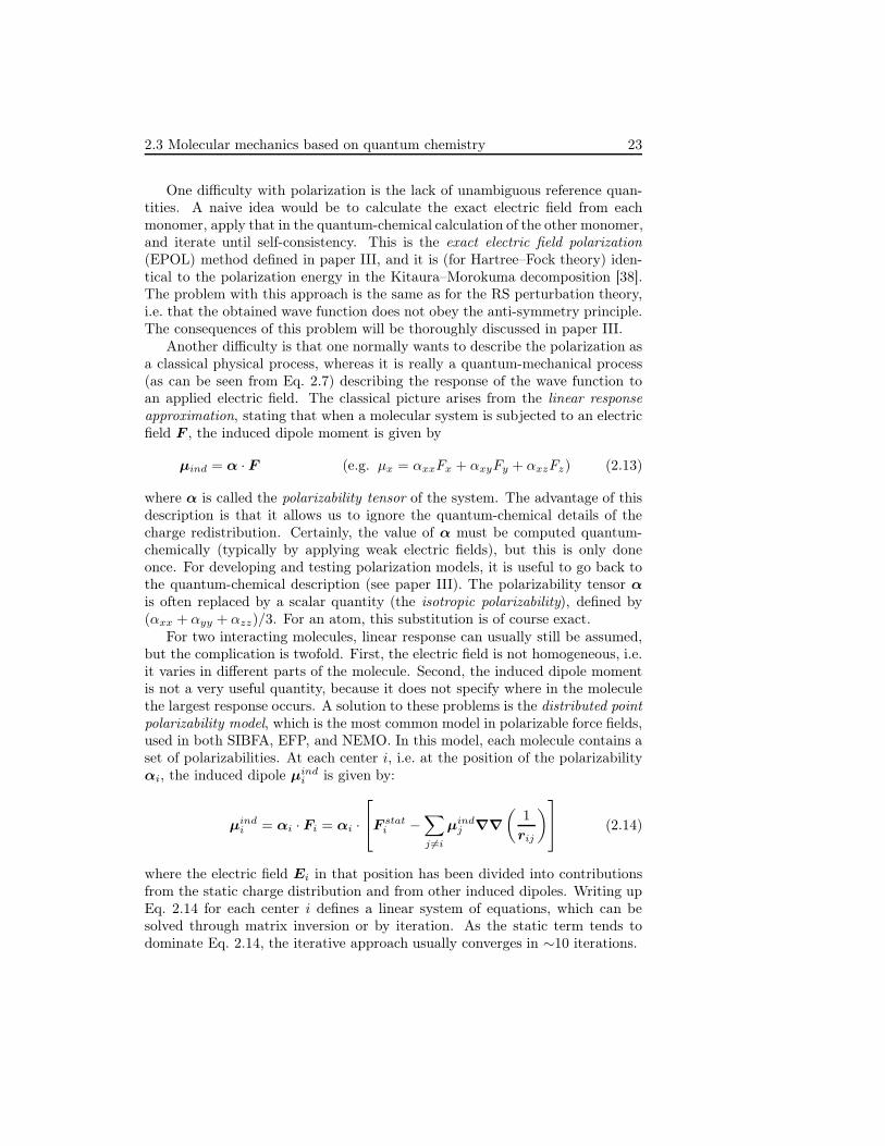
Polarization models [44] are a central theme in this thesis. The polarizationproblem is significantly more complex than the electrostatic interaction. Thereason that so much effort has been spent on improving the electrostatic interac-tion is not its complexity, but the fact that it is usually larger in magnitude andmore long-ranged and therefore more important to model accurately (anotherreason is of course the dominance of non-polarizable force fields).
2.3 Molecular mechanics based on quantum chemistry 23
One difficulty with polarization is the lack of unambiguous reference quan-tities. A naive idea would be to calculate the exact electric field from eachmonomer, apply that in the quantum-chemical calculation of the other monomer,and iterate until self-consistency. This is the exact electric field polarization(EPOL) method defined in paper III, and it is (for Hartree–Fock theory) iden-tical to the polarization energy in the Kitaura–Morokuma decomposition [38].The problem with this approach is the same as for the RS perturbation theory,i.e. that the obtained wave function does not obey the anti-symmetry principle.The consequences of this problem will be thoroughly discussed in paper III.
Another difficulty is that one normally wants to describe the polarization asa classical physical process, whereas it is really a quantum-mechanical process(as can be seen from Eq. 2.7) describing the response of the wave function toan applied electric field. The classical picture arises from the linear responseapproximation, stating that when a molecular system is subjected to an electricfield F , the induced dipole moment is given by
µind = α · F (e.g. µx = αxxFx + αxyFy + αxzFz) (2.13)
where α is called the polarizability tensor of the system. The advantage of thisdescription is that it allows us to ignore the quantum-chemical details of thecharge redistribution. Certainly, the value of α must be computed quantum-chemically (typically by applying weak electric fields), but this is only doneonce. For developing and testing polarization models, it is useful to go back tothe quantum-chemical description (see paper III). The polarizability tensor α
is often replaced by a scalar quantity (the isotropic polarizability), defined by(αxx + αyy + αzz)/3. For an atom, this substitution is of course exact.
For two interacting molecules, linear response can usually still be assumed,but the complication is twofold. First, the electric field is not homogeneous, i.e.it varies in different parts of the molecule. Second, the induced dipole momentis not a very useful quantity, because it does not specify where in the moleculethe largest response occurs. A solution to these problems is the distributed pointpolarizability model, which is the most common model in polarizable force fields,used in both SIBFA, EFP, and NEMO. In this model, each molecule contains aset of polarizabilities. At each center i, i.e. at the position of the polarizabilityαi, the induced dipole µind
i is given by:
µindi = αi · Fi = αi ·
F stati −
∑
j 6=i
µindj ∇∇
(1
rij
)
(2.14)
where the electric field Ei in that position has been divided into contributionsfrom the static charge distribution and from other induced dipoles. Writing upEq. 2.14 for each center i defines a linear system of equations, which can besolved through matrix inversion or by iteration. As the static term tends todominate Eq. 2.14, the iterative approach usually converges in ∼10 iterations.

24 Chapter 2: Intermolecular interactions
The induction energy is given by
Eind = −1
2
N∑
i=1
µi · Estati (2.15)
where the factor 1/2 comes from the fact that the (positive) work of polarizationcancels half of the energy of the dipoles in the field. Note that the energycontribution from a pair of induced dipoles is completely cancelled by the workof polarization, so Eq. 2.15 contains only the static field (but the coupling isanyway included through the values of µi).
The static field Estati may in principle come from the exact charge distribu-
tion (as in paper III), but is normally computed from the multipole expansion:
Estati = −
∑
j 6=i
[qj∇
(1
rij
)+ µj · ∇∇
(1
rij
)+ Θj · ∇∇∇
(1
rij
)...
](2.16)
where, in the simplest versions of polarizable force fields, only the first term isused.
In Eqs. 2.14 and 2.16, the contribution to the field from all surrounding cen-ters are treated equally. In practice, one often omits or damps contributionsfrom certain (typically close-lying) induced or static multipoles, but the reasonsfor doing so vary in the two cases. For the coupling between polarizabilities inEq. 2.14, the induced dipoles may become infinite at small distances (the “polar-ization catastrophe”), and the polarization can become unphysical even beforethat happens. Although it is possible to reproduce the molecular polarizabilityby a set of fully coupled atomic polarizabilities, significantly smaller values mustbe used than with an uncoupled set [94]. An alternative is to damp the dipoleinteraction tensor for overlapping charge distributions. The most used suchdamping is the one by Thole [95], sometimes reparameterized [96]. Other op-tions include omitting contributions from atoms that are directly bonded [97] orseparated by less than three bonds [53], for example. In most methods for deriv-ing polarizabilities that are based directly on quantum-chemical calculations (seebelow), the coupling is ignored between polarizabilities in the same molecule,because it is already implicitly included through the quantum-chemical calcula-tions. The explicit and implicit coupling schemes have been compared [98] andwill also be discussed in Paper V. To reduce the computational cost, it has beensuggested to omit all polarizability coupling (i.e. not only the intramolecularpart) and instead slightly enhance the charges [99] or to include the coupling tofirst order [100]. These approximations assume that the effect of the couplingis a minor part of the total effect of polarization.
On the other hand, for the response to the static field, which we will refer toas static polarization, the choice of which interactions to include in Eq. 2.16 (andpossible damping) is more a question of definition. Indeed, for a rigid molecule,it is simple to change between on one hand a representation where the static field

2.3 Molecular mechanics based on quantum chemistry 25
from multipoles in the same molecule are included in Eq. 2.16, and on the otherhand a representation where all such contributions are excluded and insteadmodeled by permanent dipoles, i.e. a “pre-polarized” molecule. Although theserepresentations give equal results, the latter can be preferable for qualitativeconclusions, as will be discussed in paper V. For a flexible molecule, the staticpolarization can be used as a way to model how the charge distribution (or themultipole representation of it) varies with changes in the molecular geometry [52,101–104].
Determining distributed point polarizabilities
The determination of distributed point polarizabilities from quantum-chemicalcalculations is more cumbersome than for multipole moments [44], mainly be-cause of two issues.
First, the response is a more complicated property. The electrostatic proper-ties are simply determined by the charge density ρ(r); and distributed multipolemoments are simply expectation values over local partitions of ρ(r). However,for fully describing the polarization of a system, we need to know the changein charge density for an arbitrary external potential. Assuming linear response,this can be expressed as
∆ρ(r) =
∫α(r, r′)V (r′)dr′, (2.17)
where V (r′) is the external potential and α(r, r′) is the charge density sus-ceptibility function, describing the change in density in one point caused by acertain electric potential in another point. A direct partitioning and “multipoleexpansion” of the charge density susceptibility function (using e.g. coupled per-turbed Hartree–Fock theory) therefore leads to both local and non-local pointpolarizabilities [105], the latter giving the induced dipole at one center causedby the electric field at another center. Such description is awkward in practice,because the number of polarizabilities varies as N2 with the number of centersN). However, if the partitioning is done properly, the non-local polarizabilitiescan be eliminated [106]. A simpler approach is to use homogeneous electricfields for the perturbation and assume from the outset that the charge densitysusceptibility function is local [76, 107].
Second, a direct analysis of ∆ρ(r) will give monopoles as well as dipoles(higher-order multipoles are normally discarded). This represents the “chargeflow” due to the polarization, which is a realistic process but cannot be modeledin a pure point-polarizability model. Therefore, they are normally convertedto point polarizabilities. As this process is of course approximate, it is advan-tageous for a partitioning scheme to give small monopole polarizabilities [108].In another context, monopole polarizabilities have been used to characterizechemical bonds [109].
The partitioning of the response can mainly be done by the same two ap-proaches as the density partitioning for multipoles. In the grid-based approach,

26 Chapter 2: Intermolecular interactions
one typically runs a large set of calculations each having a perturbing pointcharge at one grid point. The induced electric potential at that particular gridpoint [110] or at all grid points simultaneously [111, 112] is used to fit a set ofpolarizabilities up to an arbitrary multipole order. The main advantage of thisprocedure is that the set of dipole polarizabilities can be optimized to describeeffects related to higher-order polarizabilities as well. A drawback is that it isunable to assign polarizabilities reliably to “buried” atomic sites.
It was early recognized that basis-space partitioning of the response canlead to large charge flow and unphysical polarizabilities, especially for basissets containing diffuse functions [113]. The reason is the same that causes thebasis-set dependence of distributed multipoles, i.e. that when adding togetherbasis sets for each atom, the resulting basis set may be “overcomplete” (ill-conditioned). Thus, the application of even a very weak electric field can causesignificant changes in the MO coefficients without the total density being af-fected very much. As for multipoles, one solution to this problem is to use areal-space (topological) partitioning [114,115]. More computationally appealingmethods include a density fitting approach [108], a localized molecular orbitalsapproach [107], and the LoProp approach [76] (see papers II and III), in whicha more physical partitioning reduces the numerical problems and the chargeflow terms are minimized by a Lagrange multiplier approach. A quite differentapproach is to express the polarizability in terms of force operators that can bedecomposed into nuclear contributions without reference to any basis set [116].
The numerical problems can also be avoided by not performing the perturbedcalculations explicitly, as in the uncoupled Hartree–Fock approximation [117],which is also much faster. Although the molecular polarizability is not repro-duced exactly in such approaches, they may still be useful in practice, becausehigher-order molecular polarizabilities (which crucially depend on the distribu-tion method) may be important as well. Moreover, a simple scaling is oftenpossible (see paper II).
All the methods considered above are “method-consistent”, i.e. the polariz-abilities obtained at a certain quantum-chemical level (and a certain basis set)give interaction energies comparable to supermolecular results at the same level.However, it may sometimes be possible to cure deficiencies in the interactionmodel by employing polarizabilities computed at another level. For example,it has been suggested to avoid diffuse functions when computing polarizabil-ities, in order to capture some of the Pauli effects present in the condensedstate [50, 118].
Beyond point polarizabilities
As has already been mentioned, non-local (two-site) polarizabilities, monopole(charge flow) polarizabilities, and higher-order polarizabilities can be derived bysimilar methods. In fact, dipole–quadrupole polarizabilities have been found toimprove the description of the response [119]. Explicit inclusion of charge flow

2.3 Molecular mechanics based on quantum chemistry 27
does not seem to give a significant effect for most systems, as will be demon-strated in paper III. An illustrative example is given in Figure 2.3, which showsthe response of a formamide molecule with two different polarization modelswhen interacting strongly. Although the response looks quite different for themodel including charge flow, the induced electric potential around the moleculeis similar (see paper III). On the other hand, monopole polarizabilities are ex-pected to be advantageous for describing conjugated π-systems, for example.
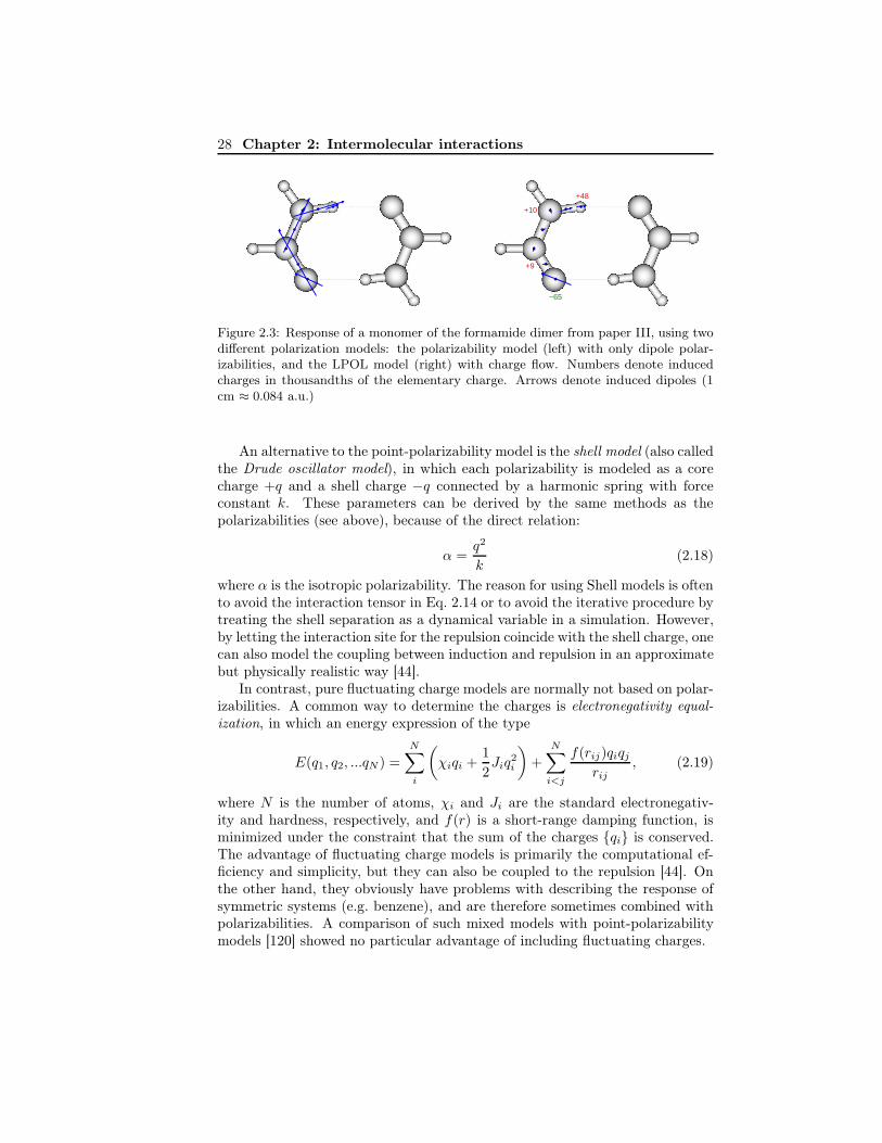
28 Chapter 2: Intermolecular interactions
+9
+10
+48
−65
Figure 2.3: Response of a monomer of the formamide dimer from paper III, using twodifferent polarization models: the polarizability model (left) with only dipole polar-izabilities, and the LPOL model (right) with charge flow. Numbers denote inducedcharges in thousandths of the elementary charge. Arrows denote induced dipoles (1cm ≈ 0.084 a.u.)
An alternative to the point-polarizability model is the shell model (also calledthe Drude oscillator model), in which each polarizability is modeled as a corecharge +q and a shell charge −q connected by a harmonic spring with forceconstant k. These parameters can be derived by the same methods as thepolarizabilities (see above), because of the direct relation:
α =q2
k(2.18)
where α is the isotropic polarizability. The reason for using Shell models is oftento avoid the interaction tensor in Eq. 2.14 or to avoid the iterative procedure bytreating the shell separation as a dynamical variable in a simulation. However,by letting the interaction site for the repulsion coincide with the shell charge, onecan also model the coupling between induction and repulsion in an approximatebut physically realistic way [44].
In contrast, pure fluctuating charge models are normally not based on polar-izabilities. A common way to determine the charges is electronegativity equal-ization, in which an energy expression of the type
E(q1, q2, ...qN ) =N∑
i
(χiqi +
1
2Jiq
2i
)+
N∑
i<j
f(rij)qiqjrij
, (2.19)
where N is the number of atoms, χi and Ji are the standard electronegativ-ity and hardness, respectively, and f(r) is a short-range damping function, isminimized under the constraint that the sum of the charges qi is conserved.The advantage of fluctuating charge models is primarily the computational ef-ficiency and simplicity, but they can also be coupled to the repulsion [44]. Onthe other hand, they obviously have problems with describing the response ofsymmetric systems (e.g. benzene), and are therefore sometimes combined withpolarizabilities. A comparison of such mixed models with point-polarizabilitymodels [120] showed no particular advantage of including fluctuating charges.
2.3 Molecular mechanics based on quantum chemistry 29
2.3.3 Dispersion
A multipole expansion of the interaction operator in the third term of Eq. 2.7leads to the following asymptotic series for the dispersion energy between twoatoms A and B:
Edisp = −C6
R6−C8
R8−C10
R10... (2.20)
where R is the interatomic distance and Cn are known as dispersion coefficients.In the well-known London formula, the series is truncated after the first termand the dispersion coefficient is estimated [4] by
C6 =3
2αAαB
(IAIBIA + IB
)(2.21)
where αX and IX are the polarizability and ionization potential of monomerX , respectively. This approach can be directly extended to molecules by usinga sum over atom–atom pairs and either treating the dispersion coefficients asadjustable parameters (as in standard force fields) or calculating them by aLondon-like formula [49].
To account for the effects of overlapping charge distributions, each term inEq. 2.20 can be damped, e.g. by the much used Tang–Toennies model [121] orby models fitted to symmetry-adapted perturbation theory [122].
Determining dispersion coefficients
A direct calculation of the distributed dispersion coefficients from quantumchemistry usually proceeds via the frequent-dependent polarizabilities α(iν).In EFP, the dispersion is described using a sum over LMO (local molecularorbital) pairs involving anisotropic polarizabilities [123]:
Edisp =∑
j∈A
∑
k∈B
∑
αβγδ
T jkαβT
jkγδ
∫ ∞
0
αjαγ(iν)αk
βδ(iν)dν, (2.22)
where T jkxx , T
jkxy , ... are elements of the dipole interaction tensor for the distance
between LMO centers j and k, and αjxx, α
jxy, ... are elements of the anisotropic
frequency-dependent polarizability tensor located at center j. For practicalreasons, one normally uses isotropic polarizabilities in the EFP dispersion, sothat Eq. 2.22 reduces to a simple sum of R−6
jk terms. Similar expressions havebeen used by others and augmented with R−8 and R−10 terms arising from thecorresponding treatment of higher-order polarizabilities [124]. Analogously, thecharge-flow polarizabilities give rise to lower-order terms (down to R−2) thatcancel at long range, but including such terms may give numerical errors [124]. Anon-expanded treatment of the dispersion, including higher-order terms as wellas overlap effects, can be formulated in terms of frequency-dependent densitysusceptibilities [125], but to a significantly higher computational cost.

30 Chapter 2: Intermolecular interactions
The calculation of frequency-dependent polarizabilities (or susceptibilities)requires at least time-dependent Hartree–Fock (TDHF) or density functionaltheory (TDDFT). Distributing the polarizabilities over the molecule can beperformed by the same type of methods as for static polarizabilities (see Sec-tion 2.3.2). A computationally simpler approach to distributed dispersion coef-ficients exploits a connection to the dipole moment of the exchange hole [126],which can also be localized using standard methods [127,128].
2.3.4 Repulsion
Similar to the case of polarization, there is no unambiguous definition of repul-sion. One possible definition is the Hartree–Fock exchange–repulsion energy.This approach is taken by the EFP and SIBFA force fields and allows for asystematic improvement of each term based on physics. Another common ap-proach, used in NEMO, is to use the repulsion as a rest term [49], defined e.g.as
Erep = Etot − Eele − Eind − Edisp. (2.23)
It is then fitted to supermolecular energies for a set of interacting dimers [129].With this definition, the repulsion will also contain overlap corrections to theinduction, dispersion, and electrostatic energies, as well as charge transfer (seebelow). The advantages of this approach are that simpler expressions can beused for all terms and that errors inherent in each term can be effectively cor-rected for, but on the other hand the transferability is not guaranteed.
The Hartree–Fock exchange–repulsion energy can be obtained by subtractingthe electrostatic energy from the Heitler–London interaction energy (or equiva-lently, by the Kitaura–Morokuma decomposition [38] scheme). It is often dividedinto an exchange contribution and a repulsion contribution [130]. The former isalways attractive and is simply the sum of exchange contributions (second termin the i, j-sum of Eq. 1.12) from orbitals on different monomers. The latter isrepulsive and always larger in absolute value, thus causing a net repulsion. Itsorigin can be qualitatively understood in terms of a depletion of electron densityin the overlap region due to the antisymmetrization [131].
The common modeling of the repulsion by a term proportional to R−12 ismainly due to computational convenience; an R−9 or R−10 dependence has alsobeen used [11]. A more realistic repulsion potential decays exponentially, as inthe Born–Mayer model:
Erep =∑
i∈A
∑
j∈B
κij exp (−αijRij) , (2.24)
where αij and κij are atom–atom parameters and Rij is the interatomic dis-tance. If needed, the potential can be modified to include the anisotropy of eachatom–atom term [132], e.g. by
Erep =∑
i∈A
∑
j∈B
exp (−αij(ωij) [Rij − ρij(ωij)]) , (2.25)

2.3 Molecular mechanics based on quantum chemistry 31
where ωij is the relative orientation of the local axes of atoms i and j, and αij
and ρij are functions of ωij . Thus, the main problem lies in determining theparameters.
Determining repulsive parameters
Asymptotically, the exchange repulsion is proportional to S2, where S is theoverlap integral of the monomer wave functions [133]. For Hartree–Fock monomerwave functions, S2 is given by
S2 =
A∑
i
B∑
j
〈ψi|ψj〉2 (2.26)
where ψi and ψj are occupied molecular orbitals (MOs) of the isolated monomersA and B.
For further analysis, it is practical to start from the perturbative defini-tion of exchange repulsion (i.e. the E(1)
exch term of Eq. 2.9), which differs fromthe Hartree–Fock exchange repulsion only at order S4 [134]. An exact expres-sion for E(1)
exch has been given [134], but more computationally feasible formulasare usually based on an (infinite) expansion in terms of overlap integrals. Fora dimer, only even powers of S occurs in the expansion and expressions forthe S2 and S4 orders have been given. By approximating the S2 expressionin various ways (e.g. the spherical Gaussian overlap approximation [135]), aparameter-free exchange-repulsion model [136] has been included in the EFPmethod. More approximate models are based directly on the squared orbitaloverlap of Eq. 2.26 [137, 138], sometimes modified by introducing an explicitdistance dependence [139,140].
Because the exact computation of S2 requires the wave functions of themonomers, it is rather impractical to use in a force field. Therefore, manymodels are instead related to the density overlap:
Ω =
∫ρA(r)ρB(r)dr (2.27)
where ρA and ρB are the electron densities of the isolated monomers. Approxi-mate proportionality between the exchange repulsion and Ω was found for bothatomic [141] and molecular dimers [87,142]. The comparison of repulsion mod-els based on orbital overlap (S2) and density overlap (Ω) is the subject of paperI.
The gain of relating the repulsion to the density overlap instead of the or-bital overlap might not be immediately apparent. However, the density overlapis significantly easier to approximate. As in the charge-penetration case, thenumber of Gaussians used to represent the molecular density can be signifi-cantly reduced [80]. The density overlap model can also be used together withdensity-fitting techniques [83]. Moreover, the integral in Eq. 2.27 is amenable to

32 Chapter 2: Intermolecular interactions
numerical integration [87]. If one divides the monomer density into atomic con-tributions, each approximated by a spherical exponentially decaying function,the overlap model provides a way to directly calculate the repulsion parame-ters in simple potentials, e.g. Eq. 2.24 (see paper I). A related approach is usedin NEMO to derive atom-wise parameters from the trace of the distributedquadrupole moments [129].
Another way of determining parameters is to place a probe atom at manydifferent positions around the molecule and fit atomic parameters (possiblyanisotropic) to the resulting exchange-repulsion energy [143]. This method maycapture some system-specific effects while still only performing monomer calcu-lations. As for the decomposed density overlap approach, accurate combinationrules are required to obtain the atom–atom properties of Eqs. 2.24 or 2.25.
Beyond additive repulsion
Perturbation theory has shown that the true exchange repulsion, in contrast tothe models above, is non-additive [144], and moreover that it couples with theinduction. This is not surprising, considering that the repulsion, like the polar-ization, influences the charge density. As an example, the charge redistributionin the water dimer caused by the mere antisymmetrization of the dimer wavefunction is shown in the left part of Fig. 2.4, with the lighter surface represent-ing a decreased and the darker an increased electron density. For comparison,the fully polarized redistribution is shown in the right part of Fig. 2.4. As canbe seen, the antisymmetrization gives a significant contribution.

2.3 Molecular mechanics based on quantum chemistry 33
Figure 2.4: Isodensity surfaces (light for negative and dark for positive) for the changein density upon formation of the water dimer. The left part shows the antisymmetrizedbut unpolarized wave function whereas the right part shows the fully polarized wavefunction.
For these reasons, one would ideally like to model the repulsion on a sim-ilar level as the polarization, that is, one would need a way to “polarize” themolecule by repulsion. However, because the repulsion is a non-classical effect,there is nothing corresponding to point-polarizabilities. One solution, whichwas recently applied in a non-additive force field [145], is to model the densitydepletion as an exchange-quadrupole. Another solution is to directly computethe coupling from orbital overlap expressions [146].
A possible approach to develop this type of models is to start from a de-scription in which one of the monomers is treated by quantum chemistry andthe other monomer (B) by a simpler model. This description is also directlyuseful for treating the influence from the environment on a quantum-chemicalcalculation [147–150], e.g. for calculating solvent effects on spectra- [151]. Theapproach is analogous to conventional QM/MM methods [152], in which electro-static (but usually not repulsive) effects are captured by embedding the systemof interest in point charges.
The repulsive effect can be modeled as a pseudopotential, which is added tothe Hamiltonian of the quantum-chemical system. Pseudopotentials were firstintroduced in studies of atoms as a way to remove the explicit treatment of thecore electrons. A common choice (for monomer A) is
VA =∑
i
di |ψBi
⟩ ⟨ψB
i | (2.28)
where the sum runs over the occupied orbitals |ψBi 〉 of monomer B and di is
a parameter which often depends on the orbital energy. For determining theparameters di, theoretical analyses exist for the pure repulsion in simple systems,but normally a fitting or qualitative arguments are applied. In this way, onecan also account for the attractive exchange (which is costly to add separately),or even the effective repulsion in Eq. 2.23. A more advanced pseudopotentialhas been derived from the variational derivative of the EFP repulsion [146].
Pseudopotentials based on the density overlap have also been developed [153,

34 Chapter 2: Intermolecular interactions
154]. The effect can also be modeled by standard density functionals [155].
2.3.5 Charge transfer
The charge-transfer term is usually described as the energy lowering due to ex-citation of electrons from the occupied orbitals of one monomer into the virtualorbitals of the other [156], in contrast to the induction energy, which involvesexcitations to the virtual orbitals of the same molecule. Obviously, as the basisset is enlarged and approaches completeness, the two virtual spaces will practi-cally coincide and the charge transfer will either vanish [39,40] or double-countthe induction energy [38] depending on the exact definition employed. Thus,the charge-transfer energy can be seen as an ill-defined part of the induction en-ergy [157], or simply be defined as the part of the interaction energy that cannotbe described when each monomer uses its own basis set. A similar definitionhas been used to compute the charge-transfer within intermolecular perturba-tion theory [157], as the standard definitions suffer from contamination fromBSSE.
It has been shown that the charge-transfer energy has an exponential de-cay with intermolecular distance (like the exchange repulsion) and that it issignificant for normal hydrogen bonds using typical basis sets [157]. Althoughone can argue that it is a mathematical artifact and could be lumped togetherwith other garbage terms, such treatment may interfere with the goal of trans-ferability. Therefore, explicit estimates of the charge-transfer energies basedon monomer properties are included in both the SIBFA and EFP methods, al-though the expressions used are remarkably different [140, 156]. Much simplerapproaches have also been devised, e.g. using a Born–Meyer term with negativesign [158].
Chapter 3
Protein–ligand affinities
Mutual molecular recognition is the starting point for almost all processes inbiological systems [159]. An enzyme must bind the correct substrate for areaction to take place, a receptor must bind the correct compound to trigger asignal, etc. From a computational point of view, this is a very difficult problem,because the protein is large, both molecules are flexible, and water (which isin itself a difficult liquid to model) plays an important role. At the same time,however, it is an intriguing problem, because it is one of the rare quantities thatare both well-defined at a microscopic level and at the same time possible tomeasure accurately experimentally.
Not surprisingly, this problem is of great interest to the pharmaceutical in-dustry, because many drugs are competitors with natural compounds in bindingto proteins. The prediction of the binding free energy of a ligand to a proteinhas been described as the Holy Grail of rational drug design [159]. For the cal-culation to be really useful in drug development, an accuracy of ∼4 kJ/mol isrequired. This can appear as an impossible wish, considering the complexity ofthe process, but in fact, several studies have reported such accuracies, althoughmethods that achieve this for an arbitrary protein–ligand complex are still faraway.
Depending on the development phase, one might have different startingpoints for the problem. Some methods, e.g. QSAR and pharmacophore model-ing, can be applied even if the structure of the protein has not been determined.Predicting the binding pose of the ligand to the protein, docking, requires thatthe structure is known. The subsequent prediction of the binding free energyis called scoring. Many types of scoring functions have been developed [159],including empirical, based on a weighted sum of simple structural properties,knowledge-based, based on a statistical analysis of known protein–ligand struc-tures, and physical, based on a potential-energy surface. Docking and scoring isnormally an interrelated process, but specific tests of scoring functions can e.g.be performed by using experimentally determined binding poses.
35

36 Chapter 3: Protein–ligand affinities
In the following, it is assumed that the binding pose is known. Moreover,to comply with the main thread of the thesis, only physical methods will bediscussed. A comparison of the accuracy of scoring functions [160] showed thata physical approach is not guaranteed to give the best results. Only if themodel includes all important effects in a balanced way and treated with as fewapproximations as possible, such distinction can be expected.
3.1 Theory
For the dissociation of a protein–ligand (PL) complex into the unbound protein(P) and ligand (L) in aqueous solution, the equilibrium constant Kd is given by
Kd =[P ][L]
[PL](3.1)
where [...] denotes the concentration. Experimentally, Kd is the concentrationof ligand necessary to make a half of the receptor sites occupied. The standardfree energy of binding (per molecule) is then defined as
∆GPL = −kBT ln(Kd/C
) (3.2)
where C is the standard concentration (1 M). The work associated with thevolume change of the process is usually negligible, so no differentiation betweenGibbs and Helmholtz free energies is done.
Based on the classical probability distribution defined in Eq. 1.25, the freeenergy is given [161] by
∆GPL = −kBT ln
(C
8π2
ZPL+SZS
ZP+SZL+S
). (3.3)
Here, each configuration integral is given by
ZX =
∫exp [−E(rX)/kBT ]drX (3.4)
where rX are the coordinates of the system X , for example all protein andsolvent coordinates in the case X = P + S. It is possible to integrate out theexplicit solvent coordinates by using the solvation free energy W (rX) for a givensolute configuration. Thus, Eq. 3.3 is equivalent to
∆GPL = −kBT ln
(C
8π2
ZPL
ZPZL
). (3.5)
where
ZX =
∫exp (− [E(rX) +W (rX)] /kBT )drX . (3.6)
This is the starting point for implicit-solvent approaches.

3.2 Path-based methods 37
For reasonably small complexes, it is possible to directly approximate theconfiguration integral in Eq. 3.6 by a sum of integrals of the predominantstates [162] found by a conformational search. Most other methods, however,rely on simulation techniques to find suitable ensembles from which the freeenergies can be extracted [163]. Usually, one distinguishes between path-basedmethods, which include sampling of various (usually unphysical) intermediatestates, and end-point methods, which only involve simulations of the free andbound states.
3.2 Path-based methods
3.2.1 Relative affinities
The most common approach to rigorously calculate the difference in binding freeenergy between two ligands is the double decoupling method [164]. It is based onthe thermodynamic cycle shown in Fig. 3.1. Instead of directly calculating thebinding affinities for the L and L′ ligands (∆GPL and ∆GPL′), one calculatesthe free energy of transforming L to L′ in the complex (∆G1) and in solution(∆G2) and uses the energy conservation to obtain
∆GPL′ − ∆GPL = ∆G1 − ∆G2 (3.7)
The connection with the partition function expressions is trivial. Using Eq. 3.3gives
∆GPL′−∆G
PL = −kBT lnZPL′+S
ZPL+S−
(−kBT ln(
ZL′+S
ZL+S
)= ∆G
1−∆G2 (3.8)
Each of the free energies ∆G1 and ∆G2 is usually calculated by free en-ergy perturbation (Eq. 1.29) or thermodynamic integration (Eq. 1.28), whereone gradually transforms one ligand into the other by Eq. 1.27. The doubledecoupling approach is a well established technique for obtaining free energydifferences between similar ligands. It has been found to give significantly bet-ter results than simple scoring functions [165]. Most applications have usedmolecular dynamics simulation [166], but Monte Carlo simulation have alsobeen used [167].
3.2.2 Absolute affinities
Calculating absolute binding affinities is a more challenging problem. It canbe addressed by a similar type of thermodynamic cycle, which is shown inFigure 3.2 [168]. Here, the dashed line indicates that the ligand does not interactwith the surroundings, i.e. it is in the gas phase. The upper right state wasintroduced later [161] as a convenient intermediate to account for the standardconcentration while still allowing for a straight-forward computation; in this
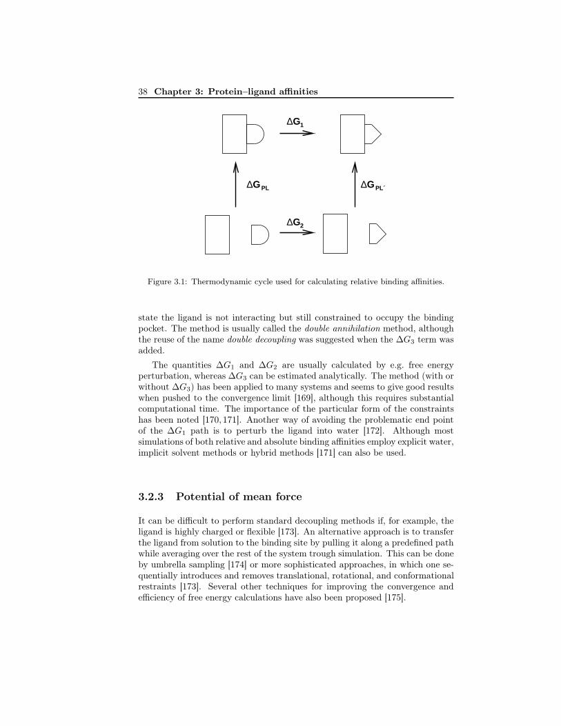
38 Chapter 3: Protein–ligand affinities
PL´∆
∆
∆
∆G G
G1
G2
PL
Figure 3.1: Thermodynamic cycle used for calculating relative binding affinities.
state the ligand is not interacting but still constrained to occupy the bindingpocket. The method is usually called the double annihilation method, althoughthe reuse of the name double decoupling was suggested when the ∆G3 term wasadded.
The quantities ∆G1 and ∆G2 are usually calculated by e.g. free energyperturbation, whereas ∆G3 can be estimated analytically. The method (with orwithout ∆G3) has been applied to many systems and seems to give good resultswhen pushed to the convergence limit [169], although this requires substantialcomputational time. The importance of the particular form of the constraintshas been noted [170, 171]. Another way of avoiding the problematic end pointof the ∆G1 path is to perturb the ligand into water [172]. Although mostsimulations of both relative and absolute binding affinities employ explicit water,implicit solvent methods or hybrid methods [171] can also be used.
3.2.3 Potential of mean force
It can be difficult to perform standard decoupling methods if, for example, theligand is highly charged or flexible [173]. An alternative approach is to transferthe ligand from solution to the binding site by pulling it along a predefined pathwhile averaging over the rest of the system trough simulation. This can be doneby umbrella sampling [174] or more sophisticated approaches, in which one se-quentially introduces and removes translational, rotational, and conformationalrestraints [173]. Several other techniques for improving the convergence andefficiency of free energy calculations have also been proposed [175].

3.3 End-point methods 39
PL ∆
∆
∆
∆G G
G1
G2
3
Figure 3.2: Thermodynamic cycle used for calculating absolute binding affinities.
3.3 End-point methods
3.3.1 Perturbations from single simulations
The procedure of performing several simulations for each ligand using various λvalues can be quite time-consuming in the double decoupling method. On theother hand, if the perturbations could be done in one step (λ = 0 → λ = 1),the relative free energies between all ligands could be computed from only onesimulation (with λ = 0). Typically, the largest problem with using one-stepperturbations is that the space needed for the addition of a new group of atomsis already occupied by the solvent or the protein. Therefore, attempts have beenmade to use an artificial reference compound containing “soft” atoms, so that theensemble generated with the reference compound is wide enough to have suffi-cient overlap with all the corresponding ensembles for the real ligands [176]. Thisapproach has been quite successful, even for structurally diverse ligands [177].Similar simplifications have also been reported [178].
Warshel et al. have also applied free-energy perturbation methods [179], buthave also found that the linear response approximation (LRA; Eq. 1.30) is agood approximation for the electrostatic contribution to the free energy [180].The neglect of the higher-order terms in Eq. 1.30 corresponds to the assumptionthat the free energy potentials with respect to an electric field are harmonic andhave equal curvature [181].

40 Chapter 3: Protein–ligand affinities
3.3.2 Linear interaction energy (LIE)
A more empirical approach to binding affinities based on LRA is the linearinteraction energy method [181]:
∆GPL = α(⟨Evdw
int
⟩PLS
−⟨Evdw
int
⟩LS
)+ β
(⟨Eele
int
⟩PLS
−⟨Eele
int
⟩LS
), (3.9)
where Evdwint and Eele
int are the Van der Waals and electrostatic parts of theinteraction energy between the ligand and the surroundings, the latter beingonly solvent in the LS ensembles but protein and solvent in the PLS ensemble.Based on the linear response approximation, the constant β was originally setto 1/2, but a direct FEP computation of the response for a wide range ofmolecules showed that β is system-dependent and deviates from 1/2 for non-ionic systems [182]. Thus a standard LIE model was devised that uses β = 0.43,0.37, and 0.33 for neutral ligands with zero, one, and two or more hydroxylgroups, respectively, and α = 0.18. This model has provided good results [183]for relative (and in some cases even absolute) binding affinities and has beenfound rather independent of the force field [184]. Nevertheless, many studiestreat both α and β as adjustable parameters. The LIE method has also beenused with implicit solvent models [185, 186].
3.3.3 MM/PBSA
In the MM/PBSA approach [187], the binding affinity is estimated by startingfrom the thermodynamic cycle in Figure 3.3 [188] and then approximating thegas-phase binding free energy by the sum of the average interaction energy andthe change in configurational entropy upon binding, i.e.
∆GPL =∆GgasPL +
(∆Gsolv
PL − ∆GsolvP − ∆Gsolv
L
)
≈⟨EMM
int
⟩PLS
− T 〈∆Sconfig〉PLS + 〈∆∆Gsolv〉PLS
(3.10)
where 〈...〉PLS indicates that the averaging is done using snapshots (typically20–100) from a simulation of the complex in solvent, usually explicit solvent.The interaction energy (EMM
int ) is computed with the water molecules removed,whereas the change in solvation energy upon binding (∆∆Gsolv) is calculatedusing an implicit solvation model. ∆S denotes the change in configurationalentropy upon binding and T is the temperature.
For the interaction energy, a standard MM force field is normally used. Apolarizable force field has also been tried [189], although without fully self-consistent treatment of the solvation. QM/MM interaction energies based onsemiempirical or density functional theory have also been used [190, 191]. Inpaper VII, an attempt to use a higher-level QM method is presented.
For the solvation energy, the most common choice is the PBSA method,i.e. the Poisson–Boltzmann (PB) method for the electrostatic part combinedwith an estimate based on the surface area for the non-polar part. Several

3.3 End-point methods 41
solv
∆GPsolv
∆
∆
∆G G
G
PL PLgas
PL
solvG∆+L
Figure 3.3: Thermodynamic cycle used in MM/PBSA.
studies have been performed with the Generalized Born method replacing PB,although these methods can sometimes give quite different results [189,192]. Inpaper VII, the polarizable continuum method (PCM) will be used, because ithas advantages in combination with a polarizable force field.
Estimating the change in configurational entropy is a very difficult problem.In fact, for computing relative affinities for similar ligands, it is probably betterto neglect this term [187], but for absolute affinities it is an essential term.It is normally computed by normal mode analysis or quasi-harmonic analysis.In the former case, one typically truncates and minimizes a small part of thecomplex and computes the vibrational, rotational, and translational entropychanges using this truncated model. For more stable results, a fixed bufferregion can be included [193]. The quasi-harmonic analysis, on the other hand,is done for the trajectories from the simulation. A problem with this approachis limited sampling and that degrees of freedom with several local minima aretreated as a single wide potential well. By using methods that treat the localminima separately, it has been found that the most important contribution tothe entropy loss comes from the energy wells becoming narrower, whereas thereduced number of conformations available is less important [194]. This is incontrast to the assumption in many simple scoring functions that the entropycan be estimated by counting the number of rotatable bonds.
The statistical-mechanical basis of the MM-PBSA method departing fromthe exact Eq. 3.5 has been described [161,195]. The most approximate assump-tion is probably that the energetic landscape of each species has an energy and

42 Chapter 3: Protein–ligand affinities
configurational volume that can be determined from a simulation, i.e.
ZX =
∫exp (− [E(rX) +W (rX)] /kBT ) drX . ≈ zint
X exp (−〈E +W 〉X/kBT ) ,
(3.11)where zX is the internal configuration integral (causing the T∆S term), and〈...〉X denotes that the average is computed for the particular species. Thismeans that the most rigorous way of computing the averages in Eq. 3.10 isby performing separate simulations of the complex, the protein and the ligand.However, as this approach usually gives severe convergence problems due to theintramolecular contributions from the protein [195], most applications have usedonly one simulation and thus have taken the protein and ligand configurationsfrom the simulation of the complex. On the other hand, separate simulationswere found to give significantly better results in at least one application [196].It has also been found that the choice of force field and solvent treatment inthe simulations have a significant effect on the results [189]. Interestingly, sim-ilar or even better results can sometimes be obtained using a single minimizedstructure [197].
3.4 Solvation
Water plays many important roles in the protein–ligand binding process. First,it acts as a dielectric continuum and screens the electrostatic interaction signifi-cantly. This is especially evident in the MM/PBSA method, where the vacuumelectrostatic energy can be over a thousand kJ/mol, but is almost completelycancelled by the solvation contribution (see paper VII). Water can also play amore direct role by forming specific hydrogen bonds with the ligand or proteinthat must be broken when the complex is formed. This is a much more diffi-cult problem to address. Unfortunately, the importance of solvation means thatthe treatment of solvation can introduce huge errors in calculations of bindingaffinities, regardless of whether an explicit or implicit solvent model is used.
There are mainly three problems with explicit water treatments. First, theyrely completely on molecular mechanics solute–water and water–water poten-tials, which can be quite different depending on the force field [198]. Second,due to the strong hydrogen-bond network in water, the sampling time (and thusthe computational load) required for adequately sampling the solvent degrees offreedom is substantial. Third, the treatment of long-range electrostatic effectsis non-trivial. Most studies employ a periodic boundary condition, for whichEwald summation seems to give rather accurate results, but this model has beenquestioned [180]. The last problem can in principle be solved by combining theexplicit model with a continuum treatment [199]. In spite of these problems,explicit models have been able to reproduce solvation energies of e.g. amino-acid models with remarkable accuracy (although differences of up to 6 kJ/moldepending on the force field were obtained) [200].

3.4 Solvation 43
Implicit water models, on the other hand, suffer from the lack of specificinteractions, e.g. hydrogen bonds. Moreover, they are usually not directly con-nected to a specific potential and are therefore dependent on other types ofparameters, typically charges and cavity radii. The advantages are the fastevaluation and the possibility of easily fitting the models directly to experi-mental solvation energies. A quantitative comparison of explicit and implicitsolvation reported good agreement in the context of binding affinities [201]. Adifferent approach to solvation is methods based on integral equation theory,e.g. the 3D-RISM method [202]. In contrast to standard implicit models, theyare based on a specific potential and can therefore incorporate some specificeffects.
Most implicit solvent models are based on the decomposition
∆Gsolv = ∆Gpolarsolv + ∆Gnon−polar
solv (3.12)
where ∆Gpolarsolv is based on roughly the same physics in the various models,
whereas ∆Gnon−polarsolv can involve quite different physical effects.
The physical motivation for Eq. 3.12 is that the solute–solvent potential en-ergy is usually based on separate electrostatic and non-electrostatic terms [203].Thus, the solvation can be described as a two-step process: first, the non-electrostatic terms of the potential are gradually turned on, creating a cavityin the solvent, and then the electrostatic term is gradually turned on. The firststep gives ∆Gnon−polar
solv and the second step gives ∆Gpolarsolv . These quantities can
be directly calculated by e.g. thermodynamic integration (Eq. 1.28), but the de-composition is ambiguous – for example, different (usually divergent) results areobtained if the steps are reversed [203]
3.4.1 Polar solvation
The polar part of the solvation is typically based on modeling the solvent as adielectric continuum, characterized by the macroscopic dielectric constant (i.e.ǫr = 80 for water). The simplest case is the solvation energy of a point chargeq in a spherical cavity with radius R. This is usually called the Born energy:
∆Gsolv =q2
2R
(1
ǫr− 1
)(3.13)
Any useful model must typically reproduce this energy. There are analogousmodels for higher multipoles, but they are typically not sufficiently accurate formodeling molecules, as these have both a complicated charge distribution anda non-spherical shape.
The basis for the continuum models is the Poisson equation:
∇ · [ǫ(r)∇φ(r)] = −4πρ(r) (3.14)
where φ(r) is the electrostatic potential at a point r, ρ(r) is the charge densityof the solute, and ǫ(r) is the position-dependent dielectric constant.
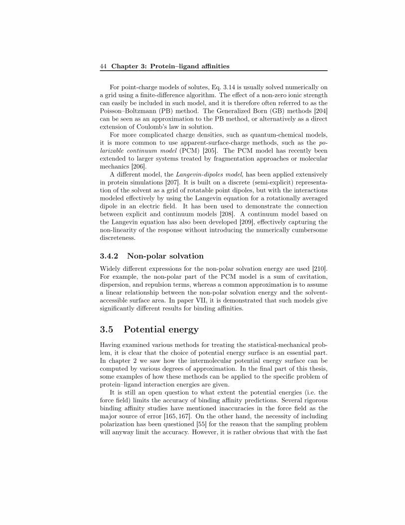
44 Chapter 3: Protein–ligand affinities
For point-charge models of solutes, Eq. 3.14 is usually solved numerically ona grid using a finite-difference algorithm. The effect of a non-zero ionic strengthcan easily be included in such model, and it is therefore often referred to as thePoisson–Boltzmann (PB) method. The Generalized Born (GB) methods [204]can be seen as an approximation to the PB method, or alternatively as a directextension of Coulomb’s law in solution.
For more complicated charge densities, such as quantum-chemical models,it is more common to use apparent-surface-charge methods, such as the po-larizable continuum model (PCM) [205]. The PCM model has recently beenextended to larger systems treated by fragmentation approaches or molecularmechanics [206].
A different model, the Langevin-dipoles model, has been applied extensivelyin protein simulations [207]. It is built on a discrete (semi-explicit) representa-tion of the solvent as a grid of rotatable point dipoles, but with the interactionsmodeled effectively by using the Langevin equation for a rotationally averageddipole in an electric field. It has been used to demonstrate the connectionbetween explicit and continuum models [208]. A continuum model based onthe Langevin equation has also been developed [209], effectively capturing thenon-linearity of the response without introducing the numerically cumbersomediscreteness.
3.4.2 Non-polar solvation
Widely different expressions for the non-polar solvation energy are used [210].For example, the non-polar part of the PCM model is a sum of cavitation,dispersion, and repulsion terms, whereas a common approximation is to assumea linear relationship between the non-polar solvation energy and the solvent-accessible surface area. In paper VII, it is demonstrated that such models givesignificantly different results for binding affinities.
3.5 Potential energy
Having examined various methods for treating the statistical-mechanical prob-lem, it is clear that the choice of potential energy surface is an essential part.In chapter 2 we saw how the intermolecular potential energy surface can becomputed by various degrees of approximation. In the final part of this thesis,some examples of how these methods can be applied to the specific problem ofprotein–ligand interaction energies are given.
It is still an open question to what extent the potential energies (i.e. theforce field) limits the accuracy of binding affinity predictions. Several rigorousbinding affinity studies have mentioned inaccuracies in the force field as themajor source of error [165, 167]. On the other hand, the necessity of includingpolarization has been questioned [55] for the reason that the sampling problemwill anyway limit the accuracy. However, it is rather obvious that with the fast

3.5 Potential energy 45
advance in computational power, the potential-energy problem will sooner orlater be dominant [1].
Most studies of protein–ligand interactions with a physical approach employstandard non-polarizable MM force fields [163, 211]. Among the polarizableforce fields with a careful treatment of each physical term, several have beenapplied to protein–ligand interactions, including the SIBFA [46, 140, 212, 213],AMOEBA [52,214], and PFF [50,215] models. Although several of these stud-ies reported a large effect of polarization on the binding affinities, it should benoted that this effect is not always attractive when the solvent is taken intoaccount [214]. Because the quantum-chemical calculations used to derive theparameters cannot be run for the full protein, the assembly of properties fromsmaller calculations (typically amino acids) is an important part of such calcu-lations [216–218] (see paper V).
A different approach to determine the potential energy is to directly exploitquantum-chemical calculations, as these are intrinsically transferable, and alsosystematically improvable [219]. Protein–ligand systems are in general too largefor a full quantum-chemical treatment. Attempts have been made to use stan-dard QM/MM methods [152] that treat only the ligand [190,220] or preferablyalso the closest residues [221] by quantum chemistry and the rest of the pro-tein by MM. However, the size of a quantum-chemical region containing theclosest residues is typically 300–800 atoms, whereas most methods that treatsdispersion interactions reasonably well (at least MP2 with a sufficiently largebasis set) are limited to ∼100 atoms. A more fruitful strategy is to decomposethe complex into smaller subsystems, which are treated more or less indepen-dently. Several such fragmentation methods have been applied to protein–ligandinteractions, including the divide-and-conquer method [222, 223], the fragmentmolecular orbital (FMO) method [224–227], the molecular fractionation withconjugate caps (MFCC) method [228–230] and related approaches [231, 232].However, only Ref. [232] has employed a reasonably accurate quantum-chemicalmethod.
A combination of the polarizable molecular mechanics and fragmentation ap-proaches will be presented in paper V, used to calculate a protein–ligand inter-action energy in paper VI, and combined with the MM/PBSA method in paperVII, providing the first protein–ligand free-energy calculations using quantum-chemical interaction energies at a reasonably high level of theory. However,an improvement of the treatment of solvation is probably necessary before animprovement in relation to experiment can be expected.

46 Chapter 3: Protein–ligand affinities

Chapter 4
Summary of the papers
4.1 Paper I: Exchange-repulsion energy
In paper I, we compare the ability of various repulsion models to reproducethe Hartree–Fock exchange-repulsion energy for a large set of molecular dimers.In particular, models based on orbital overlap, Eq. 2.26, and density overlap,Eq. 2.27, respectively, are considered.
The models contain 1 or 2 parameters, with the exception of the densityoverlap model with special scaling of certain element pairs (8 parameters) andthe parameter-free EFP method. For each model, the parameters are fitted tothe full set of dimers so that the average error is minimized.
The average error for each model is given in Table 4.1. The models assumingdirect proportionality to the orbital overlap, energy-weighted orbital overlap,and density overlap, have similar errors. Introducing another parameter tomodel the deviation from proportionality at shorter distances reduces the errorin both the orbital-overlap and density-overlap cases. However, the correctionshave different signs, because the exchange repulsion is steeper than the orbitaloverlap but less steep than the density overlap. The similar results for theSIBFA-type of correction shows that the exact functional form is not critical.
For the density overlap models, larger errors are obtained for the ethanethiol–water dimers than for the other dimers, whereas no such effect is seen for the or-bital overlap models. By comparing the contributions from each pair of molecu-lar orbitals to the orbital and density overlap, respectively, we show that aroundthe sulfur atom, destructive interference plays an important role, and this can-not be modeled by density overlap models. Therefore, it seems to be necessaryto introduce element-dependent parameters if density-overlap models should be-come as accurate as the orbital overlap models, . The EFP method performsworse than the other methods, but considering that no fitting is needed, it is auseful method for unknown systems.
47

48 Chapter 4: Summary of the papers
Table 4.1: Average error in kJ/mol for each considered model. The number of param-eters in each model is also given.
Method # param. Error
Orbital overlap:Proportional 1 1.21Proportional (energy-weighted) 1 1.10Distance-dependent 2 0.73SIBFA-type 2 0.74EFP 0 1.68Density overlap:Proportional 1 1.15Distance-dependent 2 0.97Distance- and element-dependent 8 0.60
4.2 Paper II: Multipoles and polarizabilities
In paper II, the accuracy of distributed multipoles and polarizabilities are eval-uated by comparing the static and induced electric potentials with those cal-culated from a quantum-chemical (DFT) calculation, for a set of 20 molecules.The comparison is done in 10,000 points chosen randomly in a suitable element-dependent distance range. For the evaluation of the induced potential, homo-geneous fields are applied in three orthogonal directions.
In particular, the multipoles and polarizabilities obtained by two differentapproaches are compared: the MpProp method, in which the multipoles arederived through a Mulliken-like approach [67] and the polarizabilities using theuncoupled Hartree–Fock method [117] (but scaled to give the correct molecu-lar polarizability), and the LoProp method [76], in which both the multipolesand polarizabilities are obtained using an orthogonal localized basis set andfinite-field perturbations are used for the polarizabilities. All calculations areperformed with three different basis sets.
The mean absolute error in the static and induced potentials for each moleculeis shown in Fig. 4.1. For the basis sets without diffuse functions, the MpPropmethod gives better multipole moments, regardless of the multipole level. Thereason for this is probably the better placement of the bond centers in the Mp-Prop method. On the other hand, with the basis set including diffuse functions(aug-cc-pVTZ), the LoProp method gives better results for L ≤ 3, which are themost interesting levels in practice. In particular, the MpProp method fails forlarge aromatic molecules. The LoProp method also gives better polarizabilitiesfor all basis sets, making it the preferred method for constructing intermolecularpotentials. In fact, all results become worse with the larger basis set, probablybecause the neglect of charge penetration becomes a more severe approximationas the density becomes more diffuse.
The dependence of the error on the distance from the molecular surface is

4.3 Papers III and IV: Polarization models 49
0.001
0.01
0.1
1
10M
ean
abso
lute
err
or (
kJ/m
ol)
L=1 L=2 L=3 L=4 L=5 Polar
LoProp aug−cc−pVTZMpProp aug−cc−pVTZ
LoProp cc−pVTZMpProp cc−pVTZ
LoProp 6−31G*MpProp 6−31G*
Figure 4.1: Errors in the static potential for various multipole levels L and in theinduced potential (using a field strength of 0.01 a.u.). Each point corresponds to onemolecule. A probe charge of 1 a.u. is assumed.
also tested. It is found that, for typical interaction distances, there is no gain inusing a higher multipole level than octupoles. In fact, the quadrupole level mightbe a more balanced choice when simultaneously considering the performance ofthe polarizabilities.
4.3 Papers III and IV: Polarization models
In paper III, the performance of the point-polarizability model is tested for alarge set of molecular dimers. To separately evaluate the various approximationsin the model, we use a hierarchy of models including various effects, as shownin Table 4.2. In paper IV, we introduce an additional model (ppEPOL) thatis tested partly for the same systems.
4.3.1 Densities
Because the induction energy is not an observable, we concentrate in paper IIIon the change in charge density due to the interaction. This is in itself aninteresting quantity, because it is responsible for the major part of the many-body effects – one of the reasons for using polarizable force fields at all. Variousways to analyze this induced density are used, with the most quantitative beingthe point-wise comparison of the induced electric potential used in paper II.

50 Chapter 4: Summary of the papers
Table 4.2: Summary of the considered models.
Non-expanded Intramol. Local field- Pauli Charge
Model induced density coupling inhomogeneity effects transfer
Supermolecular yes yes yes yes yes
RVS yes yes yes yes no
EPOL yes yes yes no no
LPOL yes yes no no no
Polarizabilities no no no no no
ppEPOL yes yes yes yes no
0
5
10
15
20
2 2.5 3 3.5 4 4.5
Rel
ativ
e m
ean
erro
r (%
)
H ··· O distance (Å)
EPOLLPOL
PolarizabilitiesRVS
LPOL expanded dipLPOL expanded quad
ppEPOL
Figure 4.2: Relative mean error in the induced electric potential around the waterdimer as a function of intermolecular separation.
The result for the water dimer is given in Fig. 4.2, which shows the relative er-ror compared to the supermolecular calculation for various models as a functionof the intermolecular separation. The most obvious feature is that the EPOLmodel, which uses the exact electric field as a perturbation in the quantum-chemical calculation, gives the largest error for all interesting distances. Acomparison with the RVS model shows that this is almost exclusively due tothe neglect of Pauli effects (cf. Section 2.2.2). Interestingly, the LPOL model,which also neglects Pauli effects, gives much better results. Because the onlydifference between the EPOL and LPOL is that the latter uses a locally ho-mogeneous (linearized) field, the results indicate that this approximation partlycancels the neglect of Pauli effects.
The difference between the results for the LPOL model (using quantum-chemical calculations) and the simple polarizability model is much smaller. Thisindicates that the most important approximations in the polarizability modelare not related to the actual response, but to the simplified potential that isapplied (linearized and neglecting the perturbing molecule). The curves with

4.3 Papers III and IV: Polarization models 51
the LPOL response expanded up to dipoles and quadrupoles, respectively, showthat the remaining discrepancy comes entirely from the use of only dipoles inthe polarizability model; in fact, dipole–quadrupole polarizabilities would besufficient to reproduce the LPOL result. Finally, the ppEPOL model, whichincludes Pauli effects in an approximate way, gives the best results, indicatingthat better results can be obtained without relying on the error cancellation.
A statistical analysis of the large data set shows that the water dimer israther typical for the considered systems. In general, the LPOL and polariz-ability models give lower errors (in average 9 and 10 %, respectively) than theEPOL model (16 %). However, the error cancellation between Pauli effectsand local inhomogeneity effects is not always effective. For example, in the for-mamide dimer, the error for the polarizability model is ∼90 % at the energyminimum, i.e. only slightly better than a non-polarizable model. The large dataset also confirms that the LPOL and polarizability models give similar results.In particular, the neglect of intramolecular coupling of the polarizabilities seemsto be a minor effect for the small molecules considered in this study.
4.3.2 Energies
With the introduction of the ppEPOL model in paper IV, we can also address thetotal interaction energy. In the ppEPOL model, Pauli effects are described by apseudopotential (see Section 2.3.4), which models both the exchange-repulsionenergy itself and its effect on the polarization in a consistent manner. As inthe EPOL model, the exact electric field is used. For reproducing results at anelectron-correlated level, the model must be augmented by a dispersion term(in paper IV taken as the exact expression from second-order perturbation the-ory), whereas the intramonomer correlation contributions are self-consistentlyincluded by using correlated monomer electron densities (MP2 response densi-ties).
As established in paper I, a model that is proportional to the squared overlap(S2) cannot reproduce the exchange repulsion over a large range of distances,and the same holds for standard pseudopotentials of the type in Eq. 2.28. There-fore, we introduce an S4-dependent term in the pseudopotential. Although theresulting two-parameter model could presumably be fitted in the same way asin paper I, we avoid uncertainties in the parameters by fitting the model to eachdimer separately, but still using only the zeroth-order Hartree–Fock exchange-repulsion energies. In practice, this means that we are mainly testing whetherthe polarization and its coupling to repulsion can be described by the ppEPOLmethod.
The results for the water dimer are shown in Fig. 4.3. The supermolecularcurve is well reproduced, both at the HF and MP2 level. In particular, theppEPOL model is significantly better than the uncoupled model that uses theEPOL model for the polarization and simply adds the exact Heitler–Londonenergy to account for the exchange repulsion. This shows that the coupling

52 Chapter 4: Summary of the papers
−18
−16
−14
−12
−10
−8
−6
1.8 2 2.2 2.4 2.6 2.8 3 3.2 3.4
Ene
rgy
(kJ/
mol
)
H ··· O distance (Å)
super (MP2)ppEPOL (MP2)
super (HF)ppEPOL (HF)
HLuncoupled
Figure 4.3: Intermolecular potential of the water dimer obtained with the ppEPOLmodel at the Hartree–Fock and MP2 levels and the corresponding supermolecularcurves. The results without polarization (Heitler–London; HL) and with the EPOLresult directly added to the HL energy (uncoupled) are also shown.
between polarization and repulsion is well described. The fact that this couplingin negative in sign for the minimum structures of the considered dimers suggeststhat it should rather be seen as a relaxation of the exchange-repulsion than as adamping of the polarization. However, at shorter distances the coupling becomespositive.
Encouragingly, the ppEPOL model gives good results also for the formamidedimer, which is a tough case for polarizability models. The water–chloride dimerappears slightly more difficult, but the agreement is still satisfactory. In all cases,a significant improvement of the induced density compared to the EPOL modelis also obtained. For example, the error in the induced potential decreases from128 to 6 % for the formamide dimer. Thus, the ppEPOLmodel appears as auseful model for developing and testing simpler polarization models includingcoupling between polarization and repulsion.
4.4 Paper V, VI, and VII: The PMISP method
In the last three papers, we explore a novel way of combining fragmentedquantum-chemical and molecular-mechanical calculations to compute higly ac-curate interaction energies for large systems. Paper V describes the PMISPmethod, addresses several technical details, and compares the results with fullsupermolecular calculations, as well as with other fragment approaches. PaperVI presents the first calculation of a protein–ligand interaction energy performedat a reasonably high level of theory (MP2/aug-cc-pVTZ) and investigates theaccuracy of various approximations. Paper VII combines the PMISP modelwith the polarizable continuum model (PCM) for treating solvation effects and

4.4 Paper V, VI, and VII: The PMISP method 53
R2
R1
H3
N
COON
O
H R1
H3
N CH3
N
O
H
R2
COOH3
C
O
H
N N
O
H
CH3
H3
C= +
A A1 A2 A3
Figure 4.4: Example illustrating the MFCC procedure for cutting molecule A acrossthe peptide bond and capping with –COCH3 and –NHCH3 groups. The result is twocapped fragments A1 and A2 and a concap fragment A3.
applies the resulting method in a MM/PBSA-like manner to a set of protein–ligand complexes for which the experimental binding free energies are known.
4.4.1 Methods
We try to approximate the quantum-chemical interaction energy (at a givenlevel of theory) between a large molecule A and a small molecule B. In the po-larizable multipole interaction with supermolecular pairs (PMISP) method, theinteraction energy is decomposed into classical and non-classical parts, wherethe classical part is the sum of electrostatic and induction energies given bya polarizable multipole method. Furthermore, the large molecule A is dividedinto a set of fragments Ai by the molecular fractionation with conjugate caps(MFCC) procedure [228], as illustrated in Fig. 4.4.
A previously proposed method (which we denote pairwise additive, PA) ap-proximates the total interaction energy by the sum of Ai–B interactions withthe concap interactions subtracted [228]. However, this approach neglects thenon-additivity (many-body effects) of the fragment interactions. Therefore, inthe PMISP method, the MFCC procedure is applied only for the non-classicalpart, whereas the classical part is evaluated for the whole complex, i.e. includ-ing non-additivity. The properties (multipoles and polarizabilities), on the otherhand, are assembled using the MFCC procedure.
When a full protein–ligand interaction energy is computed, the long-rangenon-classical contributions are estimated by a standard molecular mechanicsforce field, as described in paper VI. For the interaction energy in solvent (paperVII), it is assumed that only the classical part of the interaction energy isinfluenced by the solvent. A rescaling of the UAKS radii for the PCM methodis performed by fitting to experimental solvation energies for a small data set.
4.4.2 Results
In paper V, the PMISP model is tested against supermolecular calculations fora 216-atom model of avidin interacting with seven biotin analogues. Calcula-tions are performed at the HF and MP2 levels using the 6-31G* basis set. A
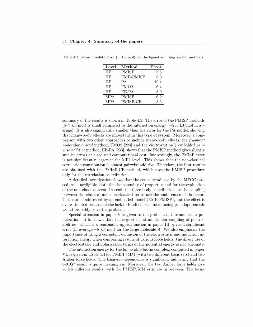
54 Chapter 4: Summary of the papers
Table 4.3: Mean absolute error (in kJ/mol) for the ligand set using several methods.
Level Method ErrorHF PMISP 5.8HF EMB-PMISP 5.0HF PA 19.4HF FMO2 6.4HF EE-PA 8.0MP2 PMISP 6.9MP2 PMISP-CE 3.3
summary of the results is shown in Table 4.3. The error of the PMISP methods(5–7 kJ/mol) is small compared to the interaction energy (−256 kJ/mol in av-erage). It is also significantly smaller than the error for the PA model, showingthat many-body effects are important in this type of system. Moreover, a com-parison with two other approaches to include many-body effects, the fragmentmolecular orbital method, FMO2 [224] and the electrostatically embedded pair-wise additive method, EE-PA [233], shows that the PMISP method gives slightlysmaller errors at a reduced computational cost. Interestingly, the PMISP erroris not significantly larger at the MP2 level. This shows that the non-classicalcorrelation contribution is almost pairwise additive. Therefore, the best resultsare obtained with the PMISP-CE method, which uses the PMISP procedureonly for the correlation contribution.
A detailed investigation shows that the error introduced by the MFCC pro-cedure is negligible, both for the assembly of properties and for the evaluationof the non-classical term. Instead, the three-body contributions to the couplingbetween the classical and non-classical terms are the main cause of the error.This can be addressed by an embedded model (EMB-PMISP), but the effect isoverestimated because of the lack of Pauli effects. Introducing pseudopotentialswould probably solve the problem.
Special attention in paper V is given to the problem of intramolecular po-larization. It is shown that the neglect of intramolecular coupling of polariz-abilities, which is a reasonable approximation in paper III, gives a significanterror (in average ∼8 kJ/mol) for the large molecule A. We also emphasize theimportance of using a consistent definition of the electrostatic and induction in-teraction energy when comparing results of various force fields: the direct use ofthe electrostatic and polarization terms of the potential energy is not adequate.
The interaction energy for the full avidin–biotin complex, computed in paperVI, is given in Table 4.4 for PMISP/MM (with two different basis sets) and twoAmber force fields. The basis-set dependence is significant, indicating that the6-31G* result is quite meaningless. Moreover, the two Amber force fields givewidely different results, with the PMISP/MM estimate in between. The term-

4.5 Conclusions and outlook 55
Table 4.4: Interaction energies (in kJ/mol) of the avidin–biotin complex with thePMISP/MM method using two different basis sets and with two Amber force fields,divided into electrostatic (Eele), induction (Eele), and non-classical (Enc) energy.
MP2/6-31G* MP2/aug-cc-pVTZ Amber ff94 Amber ff02Eele -1120 -1126 -1300 -1096Eind -190 -286 0 -113Enc 50 -8 -143 -143Etot -1261 -1419 -1443 -1353
wise comparison shows that the polarizable Amber ff02 force field significantlyunderestimates the induction energy, whereas this is partly cancelled by thenon-classical term.
The approximation to take the long-range non-classical contributions froma standard force field is evaluated by varying the cutoff distance for the PMISPtreatment. At 4 Å, this approximation gives an error of 16 kJ/mol, but this errorcan be reduced by including extra atoms for the strongest interacting groups. At7 Å, the error is negligible. Various approximations to the classical term are alsotested. It is found that MP2 properties can be replaced by B3LYP propertieswithout loss of accuracy. Octupoles and quadrupoles can be neglected outside adistance of 2 and 5 Å from the ligand, respectively, and polarizability couplingoutside of 15 Å. A significantly smaller basis set can also be used for the propertycalculations outside of 15 Å.
In the computation of binding free energies in paper VII, still for biotinanalogues binding to avidin, we encounter several problems. In particular, thedifference in non-polar solvation energies obtained with the PCM model devi-ates significantly from other estimates. Therefore, the solvent-accessible surfacearea (SASA) model is also tested. However, no matter which definition of non-polar solvation energy one uses, the results are disappointing when compared toexperimental binding affinities, giving a mean absolute deviation of ∼20 kJ/molfor relative affinities. The reason might be that the solvation model is not suffi-ciently accurate to enable the improved interaction energies to make a differencein the total results.
4.5 Conclusions and outlook
The papers presented above can be said to represent three different approachesto a common goal: the calculation of protein–ligand energies from first prin-ciples. Papers I and II represent the traditional molecular-mechanical picture,in which properties are computed separately for each monomer by quantum-chemical calculations, and then combined using simple expressions. The prop-erties in paper I are molecular orbitals or electron densities, which are somewhat

56 Chapter 4: Summary of the papers
awkward to handle in a molecular-mechanics force field, but there are alreadysuch examples [47, 83].
Papers III and especially paper IV develop a more sophisticated approach.Although it is shown that the polarizability model works well in most cases, thismodel is based on error cancellation, and thus there will always be systems forwhich it is inaccurate. Moreover, it cannot easily account for explicit couplingwith the repulsion. A solution to this is found to be a model (ppEPOL) inwhich the monomers are treated quantum-chemically but the interactions areincluded by simple expressions. Although the main purpose of this method isas a reference for models using a simpler description of the monomers (i.e. ofthe previous type), we also believe that it has a potential on its own.
Finally, the last three papers represent an approach (PMISP) in which ex-plicit quantum-chemical supermolecular calculations are performed, but onlyfor small subsystems. The many-body effects are instead modeled by a point-polarizability model. Partly, the same problem is seen here as in paper III, butas it enters only in the many-body effects, it is typically much smaller.
Which of these approaches is most suitable for achieving the goal? Surely thisdepends on the level of accuracy required and to what computational cost. Thefirst approach will always be the fastest. However, the accuracy may be limitedfor at least two reasons. First, the coupling between polarization and repulsionwill necessarily be rather approximate, and second, most such methods will haveto include some type of fitting, which may limit the transferability. The thirdapproach will always be the most accurate one, but to a higher computationalcost, allowing much fewer energy evaluations for a given problem. For the secondapproach to be computationally viable, it is essential to use simpler models forthe electric field and the dispersion energy. If this is done, such type of methodscould be a suitable compromise between the other two.
What is the accuracy needed? In my view, the best way to address thisquestion is to first use a potential-energy method that is as accurate as possibleand then, when agreement with experiment has been confirmed, gradually re-place it by computationally cheaper estimates. However, as the result of paperVII shows, this is not a trivial thing to do. Because we are currently limitedto methods that treat entropic and solvent effects at a much more approximatelevel, it is not guaranteed that an improvement is obtained. We are currentlyinvestigating the possibility of calculating a rigorous free energy with a stan-dard force field and using perturbations from the standard force field to thequantum-chemical level at the end-points [234], but the preliminary results aredisappointing: The geometries obtained with a standard force field are too dif-ferent from those that would be obtained by a quantum-chemical simulation,thus prohibiting a direct perturbational treatment. However, the use of a betterforce field for the simulations would possibly solve this problem.

Bibliography
[1] J. W. Ponder and D. A. Case, Adv. Protein Chem., 2003, 66, 27.
[2] P. A. M. Dirac, Proc. R. Soc. A, 1929, 123, 714.
[3] A. Szabo and N. S. Ostlund, Modern Quantum Chemistry, Dover Publi-cations, Mineola, 2nd ed., 1989.
[4] P. W. Atkins and R. S. Friedman, Molecular quantum mechanics, Oxforduniversity press, Oxford, 3rd ed., 1997.
[5] P. Hohenberg and W. Kohn, Phys. Rev. B, 1964, 136, 864.
[6] W. Kohn and L. J. Sham, Phys. Rev. A, 1965, 140, 1133.
[7] J. D. Head and M. C. Zerner, Adv. Quantum Chem., 1989, 20, 239.
[8] G. M. Torrie and J. P. Valleau, J. Chem. Phys., 1977, 23, 187.
[9] R. H. Swendsen and J. S. Wang, Phys. Rev. Lett., 1986, 57, 2607.
[10] R. W. Zwanzig, J. Chem. Phys., 1954, 22, 1420.
[11] A. R. Leach, Molecular Modelling: Principles and Applications, 2nd edi-tion, Pearson Education Limited, Harlow, 2001.
[12] P. Jurecka, J. Sponer, J. Cerny, and P. Hobza, Phys. Chem. Chem. Phys.,2006, 8, 1985.
[13] S. Grimme, J. Chem. Phys., 2003, 118, 9095.
[14] R. A. Bachorz, F. A. Bischoff, S. Höfener, W. Klopper, P. Ottiger, R. Leist,J. A. Frey, and S. Leutwyler, Phys. Chem. Chem. Phys., 2008, 10, 2758.
[15] J.-P. Piquemal, A. Marquez, O. Parisel, and C. Giessner-Prettre, J. Com-put. Chem., 2005, 26, 1052.
[16] J. Cerny and P. Hobza, Phys. Chem. Chem. Phys., 2007, 9, 5291.
57

58 BIBLIOGRAPHY
[17] C. Diedrich, A. Lüchow, and S. Grimme, J. Chem. Phys., 2005, 123,184106.
[18] F. B. van Duijneveldt, J. G. C. M. van Duijneveldt-van de Rijdt, and J. H.van Lenthe, Chem. Rev., 1994, 94, 1873.
[19] S. F. Boys and F. Bernardi, Molecular Physics, 1970, 19, 553.
[20] G. Karlström and A. Sadlej, Theor. Chim. Acta, 1982, 61, 1.
[21] F. B. van Duijneveldt in Molecular Interactions, ed. S. Scheiner; Wiley,Chichester, 1997; p. 81.
[22] O. Marchetti and H.-J. Werner, Phys. Chem. Chem. Phys., 2008, 10, 3400.
[23] A. Halkier, W. Klopper, T. Helgaker, P. Jorgensen, and P. R. Taylor, J.Chem. Phys., 1999, 111, 9157.
[24] A. Halkier, T. Helgaker, P. Jørgensen, W. Klopper, H. Koch, J. Olsen,and A. K. Wilson, Chem. Phys. Letters, 1998, 286, 243.
[25] F.-M. Tao and Y.-K. Pan, J. Chem. Phys., 1992, 97, 4989.
[26] W. Klopper and W. Kutzelnigg, Chem. Phys. Letters, 1987, 134, 17.
[27] H. Fliegl, W. Klopper, and C. Hättig, J. Chem. Phys., 2005, 122, 084107.
[28] T. B. Adler, G. Knizia, and H.-J. Werner, J. Chem. Phys., 2007, 127,221106.
[29] K. E. Riley and P. Hobza, J. Phys. Chem. A, 2007, 111, 8257.
[30] A. D. Buckingham, Adv. Chem. Phys., 1967, 12, 107.
[31] M. Ziólkowski, S. J. Grabowski, and J. Leszczynski, J. Phys. Chem. A,2006, 110, 6514.
[32] A. J. Stone, The Theory of Intermolecular Forces, Oxford UniversityPress, Oxford, 1st ed., 1996.
[33] B. Jeziorski, R. Moszynski, and K. Szalewicz, Chem. Rev., 1994, 94, 1887.
[34] I. C. Hayes and A. J. Stone, Mol. Phys., 1984, 53, 69.
[35] K. Szalewicz, K. Patkowski, and B. Jeziorski, Struct. Bond., 2005, 116,43.
[36] M. Gutowski, G. Chalasinski, and J. van Duijneveldt-van de Rijdt, Int.J. Quantum Chem., 1984, 26, 971.
[37] H. L. Williams, E. M. Mas, K. Szalewicz, and B. Jeziorski, J. Chem. Phys.,1995, 103, 7374.

BIBLIOGRAPHY 59
[38] K. Kitaura and K. Morokuma, Int. J. Quantum Chem., 1976, 10, 325.
[39] P. S. Bagus, K. Hermann, and C. W. J. Bauschlicher, J. Chem. Phys.,1984, 80, 4378.
[40] W. J. Stevens and W. H. Fink, Chem. Phys. Letters, 1987, 139, 15.
[41] W. Chen and M. S. Gordon, J. Phys. Chem., 1996, 100, 14316.
[42] R. F. Frey and E. R. Davidson, J. Chem. Phys., 1989, 90, 5555.
[43] W. Cornell, P. Cieplak, C. Bayly, I. Gould, K. M. Merz, D. Ferguson,D. Spellmeyer, T. Fox, J. Caldwell, and P. Kollman, J. Am. Chem. Soc.,1995, 117, 5179.
[44] S. W. Rick and S. J. Stuart in Reviews in Computational Chemistry, ed.K. B. Lipowitz and D. B. Boyd, Vol. 18; Wiley-VCH, New York, 2002;p. 89.
[45] D. P. Geerke and W. F. van Gunsteren, J. Phys. Chem. B, 2007, 111,6425.
[46] N. Gresh, G. A. Cisneros, T. A. Darden, and J.-P. Piquemal, J. Chem.Theory. Comput., 2007, 3, 1960.
[47] M. S. Gordon, M. A. Freitag, P. Bandyopadhyay, J. H. Jensen, V. Kairys,and W. J. Stevens, J. Phys. Chem. A, 2001, 105, 293.
[48] A. Wallqvist and G. Karlström, Chem. Scr. A., 1989, 29, 131.
[49] O. Engkvist, P.-O. Åstrand, and G. Karlström, Chem. Rev., 2000, 100,4087.
[50] G. A. Kaminski, H. A. Stern, B. J. Berne, and R. A. Friesner, J. Phys.Chem. A, 2004, 108, 621–627.
[51] A. G. Donchev, V. D. Ozrin, M. V. Subbotin, O. V. Tarasov, and V. I.Tarasov, Proc. Natl. Acad.. Sci., 2005, 102, 7829.
[52] P. Ren and J. W. Ponder, J. Comput. Chem., 2002, 23, 1497.
[53] P. Cieplak, J. Caldwell, and P. Kollman, J. Comput. Chem., 2001, 22,1048.
[54] S. Patel and C. L. Brooks III, J. Comput. Chem., 2004, 25, 1.
[55] A. Warshel, M. Kato, and A. V. Pisliakov, J. Chem. Theory. Comput.,2007, 3, 2034.
[56] T. A. Halgren and W. Damm, Curr. Opin. Struct. Biol., 2001, 11, 236.
60 BIBLIOGRAPHY
[57] C. J. F. Böttcher, O. C. van Belle, P. Bordewijk, and A. Rip, Theoryof Electric Polarization, vol. 1, Elsevier Scientific Publishing Company,Amsterdam, 2nd ed., 1973.
[58] E. Sigfridsson and U. Ryde, J. Comput. Chem., 1998, 19, 377.
[59] C. Chipot, J. G. Ángyán, G. G. Ferenczy, and H. A. Scheraga, J. Phys.Chem., 1993, 97, 6628.
[60] C. I. Bayly, P. Cieplak, W. D. Cornell, and P. A. Kollman, J. Phys. Chem.,1993, 97, 10269.
[61] R. C. A., J. W. Essex, and W. G. Richards, J. Am. Chem. Soc., 1992,114, 9075.
[62] P. Söderhjelm and U. Ryde, J. Comput. Chem., 2008, p. DOI:10.1002/jcc.21097.
[63] D. E. Williams, J. Comput. Chem., 1988, 9, 745.
[64] R. S. Mulliken, J. Chem. Phys., 1955, 23, 1833.
[65] P.-O. Löwdin, J. Chem. Phys., 1950, 18, 365.
[66] A. J. Stone and M. Alderton, Mol. Phys., 1985, 56, 1047.
[67] G. Karlström in Proceeding of fifth seminar on Computational Methodsin Quantum Chemistry, ed. P. T. van Duijnen and W. C. Nieuwpoort;Laboratory of Chemical Physics, University of Groningen, Groningen, TheNetherlands, 1981; p. 353.
[68] F. Vigné-Maeder and P. Claverie, J. Chem. Phys., 1988, 88, 4934.
[69] A. Reed, L. Curtiss, and F. Weinhold, Chem. Rev., 1988, 88, 899.
[70] R. F. W. Bader, Atoms in Molecules: A quantum theory, Oxford Press,Oxford, 1990.
[71] R. F. W. Bader, Chem. Rev., 1991, 91, 893.
[72] P. L. A. Popelier, Atoms in Molecules: An introduction, Pearson, London,2000.
[73] J. Pilmé and J.-P. Piquemal, J. Comput. Chem., 2008, 29, 1440.
[74] A. J. Stone and M. Alderton, J. Chem. Theory. Comput., 2005, 1, 1128.
[75] J. Cioslowski, J. Am. Chem. Soc., 1989, 111, 8333.
[76] L. Gagliardi, R. Lindh, and G. Karlström, J. Chem. Phys., 2004, 121,4494.

BIBLIOGRAPHY 61
[77] M. Rafat and P. L. A. Popelier, J. Comput. Chem., 2007, 28, 832.
[78] G. Náray-Szabó and G. G. Ferenczy, Chem. Rev., 1995, 95, 829.
[79] G. G. Hall and C. M. Smith, Int. J. Quantum Chem., 1984, 25, 881.
[80] R. J. Wheatley and J. B. O. Mitchell, J. Comput. Chem., 1994, 15, 1187.
[81] K. Strasburger, Computers Chem., 1998, 22, 7.
[82] G. A. Cisneros, J.-P. Piquemal, and T. A. Darden, J. Chem. Phys., 2005,123, 044109.
[83] J.-P. Piquemal, G. A. Cisneros, P. Reinhardt, N. Gresh, and T. A. Darden,J. Chem. Phys., 2006, 124, 104101.
[84] G. A. Cisneros, J.-P. Piquemal, and T. A. Darden, J. Chem. Phys., 2006,125, 184101.
[85] G. A. Cisneros, D. Elking, J.-P. Piquemal, and T. A. Darden, J. Phys.Chem. A, 2007, 111, 12049.
[86] B. I. Dunlap, J. W. D. Connolly, and J. R. Sabin, J. Chem. Phys., 1979,71, 4993.
[87] A. Gavezzotti, J. Phys. Chem. B, 2003, 107, 2344.
[88] Y. G. Ma and P. Politzer, J. Chem. Phys., 2004, 120, 8955.
[89] A. Volkov, T. S. Koritsanszky, and P. Coppens, Chem. Phys. Letters, 2004,391, 170.
[90] A. Volkov and P. Coppens, J. Comput. Chem., 2004, 25, 921.
[91] V. Kairys and J. H. Jensen, Chem. Phys. Letters, 1999, 315, 140.
[92] M. A. Freitag, M. S. Gordon, J. H. Jensen, and W. J. Stevens, J. Chem.Phys., 2000, 112, 7300.
[93] J.-P. Piquemal, N. Gresh, and C. Giessner-Prettre, J. Phys. Chem. A,2003, 107, 10353.
[94] J. Applequist, J. R. Carl, and K.-K. Fung, J. Am. Chem. Soc., 1972, 94,2952.
[95] B. T. Thole, Chem. Phys., 1981, 59, 341.
[96] M. Masia, M. Probst, and R. Rey, J. Chem. Phys., 2005, 123, 164505.
[97] A. Warshel and M. Levitt, J. Mol. Biol., 1976, 103, 227.

62 BIBLIOGRAPHY
[98] S. Nakagawa, P. Mark, and H. Ågren, J. Chem. Theory. Comput., 2007,3, 1947.
[99] T. Straatsma and J. McCammon, Molecular Simulation, 1990, 5, 181.
[100] G. A. Kaminski, R. A. Friesner, and R. Zhou, J. Comput. Chem., 2003,24, 267.
[101] O. Engkvist, P.-O. Åstrand, and G. Karlström, J. Phys. Chem., 1996,100, 6950.
[102] A. Holt and G. Karlström, J. Comput. Chem., 2008, 29, 1084.
[103] A. Holt and G. Karlström, J. Comput. Chem., 2008, 29, 1905.
[104] T. D. Rasmussen, P. Ren, J. W. Ponder, and F. Jensen, Int. J. QuantumChem., 2007, 107, 1390.
[105] A. J. Stone, Mol. Phys., 1985, 56, 1065.
[106] C. R. Le Sueur and A. J. Stone, Mol. Phys., 1994, 83, 293.
[107] D. R. Garmer and W. J. Stevens, J. Phys. Chem., 1989, 93, 8263.
[108] A. J. Misquitta and A. J. Stone, J. Chem. Phys., 2006, 124, 024111.
[109] A. Holt and G. Karlström, Chem. Phys. Letters, 2007, 436, 297.
[110] N. Celebi, J. G. Ángyán, F. Dehez, C. Millot, and C. Chipot, J. Chem.Phys., 2000, 112, 2709.
[111] S. Nakagawa and N. Kosugi, Chem. Phys. Letters, 1993, 210, 180.
[112] G. J. Williams and A. J. Stone, J. Chem. Phys., 2003, 119, 4620.
[113] C. R. Le Sueur and A. J. Stone, Mol. Phys., 1993, 78, 1267.
[114] J. G. Ángyán, G. Jansen, M. Loos, C. Hättig, and B. A. Heß, Chem. Phys.Letters, 1994, 219, 267.
[115] F. Dehez, C. Chipot, C. Millot, and J. G. Ángyán, Chem. Phys. Letters,2001, 338, 180.
[116] M. Ferraro, M. Caputo, and P. Lazzeretti, J. Chem. Phys., 1988, 109,2987.
[117] G. Karlström, Theor. Chim. Acta, 1982, 60, 535.
[118] A. Serr and R. R. Netz, Int. J. Quantum Chem., 2006, 106, 2960.
[119] A. Holt and G. Karlström, J. Comput. Chem., 2008, 29, 2033.

BIBLIOGRAPHY 63
[120] J.-P. Piquemal, R. Chelli, P. Procacci, and N. Gresh, J. Phys. Chem. A,2007, 111, 8170.
[121] K. T. Tang and Toennies, J. Chem. Phys., 1984, 80, 3726.
[122] M. P. Hodges and A. J. Stone, Mol. Phys., 2000, 98, 275.
[123] I. Adamovic and M. S. Gordon, Mol. Phys., 2005, 103, 379.
[124] G. J. Williams and A. J. Stone, J. Chem. Phys., 2003, 119, 4620.
[125] A. J. Misquitta, B. Jeziorski, and K. Szalewicz, Phys. Rev. Lett., 2003,91, 033201.
[126] A. D. Becke and E. R. Johnson, J. Chem. Phys., 2005, 122, 154104.
[127] E. R. Johnson and A. D. Becke, J. Chem. Phys., 2005, 123, 024101.
[128] A. Öhrn and G. Karlström, J. Phys. Chem. A, 2007, 111, 10468.
[129] S. Brdarski and G. Karlström, J. Phys. Chem. A, 1998, 102, 8182–8192.
[130] E. Fraschini and A. J. Stone, J. Comput. Chem., 1998, 19, 847.
[131] E. J. Baerends in Cluster Models for Surface and Bulk Phenomena, ed.G. Pacchione, P. S. Bagus, and F. Parmigiani; Plenum, New York, 1992.
[132] A. J. Stone and S. L. Price, J. Phys. Chem., 1988, 92, 3325.
[133] H. Margenau and N. R. Kestner, Theory of Intermolecular Forces, Perg-amon, Oxford, 1969.
[134] B. Jeziorski, M. Bulski, and L. Piela, Int. J. Quantum Chem., 1976, 10,281.
[135] J. H. Jensen, J. Chem. Phys., 1996, 104, 7795.
[136] J. Jensen and M. S. Gordon, Mol. Phys., 1996, 89, 1313.
[137] A. Wallqvist and G. Karlström, Chem. Scripta, 1989, 29A, 131.
[138] N. Gresh, P. Claverie, and A. Pullman, Int. J. Quantum Chem., 1986, 29,101.
[139] J. N. Murrell and J. J. N. Teixeiras-Dias, Mol. Phys., 1970, 19, 521.
[140] N. Gresh, J.-P. Piquemal, and M. Krauss, J. Comput. Chem., 2005, 26,1113.
[141] Y. S. Kim, S. K. Kim, and W. D. Lee, Chem. Phys. Letters, 1981, 80,574.
64 BIBLIOGRAPHY
[142] I. Nobeli, S. L. Price, and R. J. Wheatley, Mol. Phys., 1998, 95, 525.
[143] A. J. Stone and C.-S. Tong, J. Comput. Chem., 1994, 15, 1377.
[144] R. Moszynski, P. E. S. Wormer, B. Jeziorski, and A. van der Avoird, J.Chem. Phys., 1995, 103, 8058.
[145] E. M. Mas, R. Bukowski, and K. Szalewicz, J. Chem. Phys., 2003, 118,4386.
[146] J. H. Jensen, J. Chem. Phys., 2001, 114, 8775.
[147] M. Gutowski, M. Kakol, and L. Piela, Int. J. Quantum Chem., 1983, 23,1843–1853.
[148] Z. Barandiarán and L. Seijo, J. Chem. Phys., 1988, 89, 5739–5746.
[149] S. Huzinaga, J. Mol. Struc.(Theochem), 1991, 234, 51–73.
[150] I. Panas, Chem. Phys. Letters, 1993, 201, 255–260.
[151] A. Öhrn and G. Karlström, Mol. Phys., 2006, 104, 3087–3099.
[152] H. M. Senn and W. Thiel, Curr. Opin. Chem. Biol., 2007, 11, 182.
[153] E. Valderrama and R. J. Wheatley, J. Comput. Chem., 2003, 24, 2075.
[154] G. A. Cisneros, J.-P. Piquemal, and T. A. Darden, J. Chem. Phys., 2006,125, 184101.
[155] J. Neugebauer, M. J. Louwerse, E. J. Baerends, and T. A. Wesolowski, J.Chem. Phys., 2005, 122, 094115.
[156] H. Li, M. S. Gordon, and J. H. Jensen, J. Chem. Phys., 2006, 124, 214108.
[157] A. J. Stone, Chem. Phys. Letters, 1993, 211, 101.
[158] D. Hagberg, G. Karlström, B. O. Roos, and L. Gagliardi, J. Am. Chem.Soc., 2005, 127, 14250.
[159] H. Gohlke and G. Klebe, Angew. Chem. Int. Ed.., 2002, 41, 2644.
[160] P. Ferrara, H. Gohlke, D. J. Price, G. Klebe, and C. L. Brooks, III, J.Med. Chem., 2004, 47, 3032.
[161] M. K. Gilson, J. A. Given, B. L. Bush, and J. A. McCammon, Biophys.Jour., 1997, 72, 1047.
[162] C.-E. Chang and M. K. Gilson, J. Am. Chem. Soc., 2004, 126, 13156.
[163] M. K. Gilson and H.-X. Zhou, Annu. Rev. Biophys. Biomol. Struct., 2007,36, 21.
BIBLIOGRAPHY 65
[164] B. L. Tembe and J. A. McCammon, Comput. Chem., 1984, 8, 281.
[165] D. A. Pearlman and P. S. Charifson, J. Med. Chem., 2001, 44, 3417.
[166] C. Oostenbrink and W. F. van Gunsteren, Proteins: Struct. Funct. Bioin-formatics, 2004, 54, 237.
[167] J. W. Essex, D. L. Severance, J. Tirado-Rives, and W. L. Jorgensen, J.Phys. Chem. B, 1997, 101, 9663.
[168] W. L. Jorgensen, J. K. Buckner, S. Boudon, and J. Tirado-Rives, J. Chem.Phys., 1988, 89, 3742.
[169] H. Fujitani, Y. Tanida, M. Ito, G. Jayachandran, C. D. Snow, M. R.Shirts, E. J. Sorin, and V. S. Pande, J. Chem. Phys., 2005, 123, 084108.
[170] S. Boresch, F. Tettinger, M. Leitgeb, and M. Karplus, J. Phys. Chem. B,2003, 107, 9535.
[171] J. Wang, Y. Deng, and B. Roux, Biophys. Jour., 2006, 91, 2798.
[172] V. Helms and R. C. Wade, Proteins: Struct. Funct. Genet., 1998, 32, 381.
[173] W. Hyang-June and B. Roux, Proc. Natl. Acad.. Sci., 2005, 102, 6825.
[174] M. S. Lee and M. A. Olson, Biophys. Jour., 2006, 90, 864.
[175] T. Rodinger and R. Pomès, Curr. Opin. Struct. Biol., 2005, 15, 164.
[176] C. Oostenbrink and W. F. van Gunsteren, Proteins: Struct. Funct. Bioin-formatics, 2004, 54, 237.
[177] C. Oostenbrink and W. F. van Gunsteren, Proc. Natl. Acad.. Sci., 2005,102, 6750.
[178] R. J. Radmer and P. A. Kollman, J. Comput.-Aid. Mol. Design, 1998, 12,215.
[179] F. S. Lee, Z.-T. Chu, M. B. Bolger, and A. Warshel, Protein Engineering,1992, 5, 215.
[180] Y. Y. Sham, Z. T. Chu, H. Tao, and A. Warshel, Proteins: Struct. Funct.Genet., 2000, 39, 393.
[181] J. Åqvist, C. Medina, and J.-E. Samuelsson, Protein Engineering, 1994,7, 385.
[182] J. Åqvist and T. Hansson, J. Phys. Chem., 1996, 100, 9512.
[183] J. Åqvist, V. B. Luzhkov, and B. O. Brandsdal, Acc. Chem. Res., 2002,35, 358.

66 BIBLIOGRAPHY
[184] M. Almlöf, B. O. Brandsdal, and J. Åqvist, J. Comput. Chem., 2004, 25,1242.
[185] R. Zhou, R. A. Friesner, A. Ghosh, R. C. Rizzo, W. L. Jorgensen, andR. M. Levy, J. Phys. Chem. B, 2001, 105, 10388.
[186] M. N. J. Carlsson, M. Andér and J. Åqvist, J. Phys. Chem. B, 2006, 110,12034.
[187] P. A. Kollman, I. Massova, C. Reyes, B. Kuhn, S. Huo, L. Chong, M. Lee,T. Lee, Y. Duan, W. Wang, O. Donini, P. Cieplak, J. Srinivasan, D. A.Case, and T. E. Cheatham, Acc. Chem. Res., 2000, 33, 889.
[188] J. Wang, P. Morin, W. Wang, and P. A. Kollman, J. Am. Chem. Soc.,2001, 123, 5221.
[189] A. Weis, K. Katebzadeh, P. Söderhjelm, I. Nilsson, and U. Ryde, J. Med.Chem., 2006, 49, 6596.
[190] F. Gräter, S. M. Schwarzl, A. Dejaegere, S. Fischer, and J. C. Smith, J.Phys. Chem. B, 2005, 109, 10474.
[191] M. Wang and C. F. Wong, J. Chem. Phys., 2007, 126, 026101.
[192] M. Kaukonen, P. Söderhjelm, J. Heimdal, and U. Ryde, J. Phys. Chem.B, 2008, 112, 12537.
[193] J. Kongsted and U. Ryde, J. Comput.-Aid. Mol. Design, 2008, DOI:10.1007/s10822-008-9238-z.
[194] C. A. Chang, W. Chen, and M. K. Gilson, Proc. Natl. Acad.. Sci., 2007,104, 1534.
[195] J. M. J. Swanson, R. H. Henchman, and J. A. McCammon, Biophys.Jour., 2004, 86, 67.
[196] D. A. Pearlman, J. Med. Chem., 2005, 48, 7796.
[197] B. Kuhn, P. Gerber, T. Schulz-Gasch, and M. Stahl, J. Med. Chem., 2005,48, 4040.
[198] J. M. Hermida-Ramón, S. Brdarski, G. Karlström, and U. Berg, J. Com-put. Chem., 2002, 24, 161.
[199] M. S. Lee and M. A. Olson, J. Phys. Chem. B, 2005, 109, 5223.
[200] M. R. Shirts, J. W. Pitera, W. C. Swope, and V. S. Pande, J. Chem.Phys., 2003, 119, 5740.
[201] L. Y. Zhang, E. Gallicchio, and R. A. Friesner, J. Comput. Chem., 2001,22, 591.
BIBLIOGRAPHY 67
[202] D. Beglov and B. Roux, J. Phys. Chem. B, 1997, 101, 7821.
[203] B. Roux and T. Simonson, J. Chem. Phys., 2006, 124, 084905.
[204] D. Bashford and D. A. Case, Annu. Rev. Phys. Chem., 2000, 51, 129.
[205] S. Miertus, E. Scrocco, and J. Tomasi, Chem. Phys., 1981, 55, 117.
[206] H. Li, C. S. Pomelli, and J. H. Jensen, Theor. Chem. Acc., 2003, 109, 71.
[207] S. T. Russell and A. Warshel, J. Mol. Biol., 1985, 185, 389.
[208] A. Papazyan and A. Warshel, J. Phys. Chem. B, 1997, 101, 11254.
[209] L. Sandberg, R. Casemyr, and O. Edholm, J. Phys. Chem. B, 2002, 106,7889.
[210] F. J. Luque, C. Curutchet, J. Munoz-Muriedas, A. Bidon-Chanal,I. Soteras, A. Morreale, J. L. Gelpi, and M. Orozco, Phys. Chem. Chem.Phys., 2003, 5, 3827.
[211] N. Huang, C. Kalyanaraman, K. Bernacki, and M. P. Jacobson, Phys.Chem. Chem. Phys., 2006, 8, 5166.
[212] J. Antony, J.-P. Piquemal, and N. Gresh, J. Comput. Chem., 2005, 26,1131.
[213] C. Roux, N. Gresh, L. E. Perera, J.-P. Piquemal, and L. J. Salmon, J.Comput. Chem., 2007, 28, 938.
[214] D. Jiao, P. A. Golubkov, T. A. Darden, and P. Ren, Proc. Natl. Acad..Sci., 2008, 105, 6290.
[215] J. R. Maple, Y. Cao, W. Damm, T. A. Halgren, G. A. Kaminski, L. Y.Zhang, and R. A. Friesner, J. Chem. Theory. Comput., 2005, 1, 694.
[216] N. Gresh, A. Pullman, and P. Claverie, Theor. Chim. Acta, 1985, 67, 11.
[217] N. Gresh, P. Claverie, and A. Pullman, Theor. Chim. Acta, 1984, 66, 1.
[218] P. A. Molina, H. Li, and J. H. Jensen, J. Comput. Chem., 2003, 24, 1971.
[219] K. Raha, M. B. Peters, B. Wang, N. Yu, A. M. Wollacott, L. M. Wester-hoff, and K. M. Merz, Drug Discovery Today, 2007, 12, 731.
[220] A. E. Cho, V. Guallar, B. J. Berne, and R. Friesner, J. Comput. Chem.,2005, 26, 915.
[221] A. Khandelwal, V. Lukacova, D. Comez, D. M. Kroll, S. Raha, andS. Balaz, J. Med. Chem., 2005, 48, 5437.

68 BIBLIOGRAPHY
[222] W. Yang, Phys. Rev. Lett., 1991, 66, 1438.
[223] K. Raha and K. M. Merz, J. Am. Chem. Soc., 2004, 126, 1020.
[224] K. Kitaura, E. Ikeo, T. Asada, T. Nakano, and M. Uebayasi, Chem. Phys.Letters, 1999, 313, 701.
[225] K. Fukuzawa, Y. Mochizuki, S. Tanaka, K. Kitaura, and T. Nakano, J.Phys. Chem. B, 2006, 110, 16102.
[226] I. Nakanishi, D. G. Fedorov, and K. Kitaura, Proteins: Struct. Funct.Bioinformatics, 2007, 68, 145.
[227] D. G. Fedorov and K. Kitaura, J. Phys. Chem. A, 2007, 111, 6904.
[228] D. W. Zhang and J. Z. H. Zhang, J. Chem. Phys., 2003, 119, 3599.
[229] D. W. Zhang, Y. Xiang, M. Gao, and J. Z. H. Zhang, J. Chem. Phys.,2004, 120, 1145.
[230] D. W. Zhang, Y. Xiang, and J. Z. H. Zhang, J. Phys. Chem. B, 2003,107, 12039.
[231] R. P. A. Bettens and A. M. Lee, J. Phys. Chem. A, 2006, 110, 8777.
[232] R. P. A. Bettens and A. M. Lee, Chem. Phys. Letters, 2007, 449, 341.
[233] E. E. Dahlke and D. G. Truhlar, J. Chem. Theory. Comput., 2007, 3, 46.
[234] T. H. Rod and U. Ryde, Phys. Rev. Lett., 2005, 94, 138302.