a framework for the development of bus service reliability...

Australasian Transport Research Forum 2013 Proceedings 2-4 October 2013, Brisbane, Australia

1

A Framework for the Development of Bus Service Reliability Measures

Zhenliang Ma*, Luis Ferreira, Mahmoud Mesbah

School of Civil Engineering, The University of Queensland, Brisbane, QLD 4072, Australia

*Correspondence Author Email: [email protected]

Abstract

Reliability of transit service has been recognized as a significant determinant of quality of service. Numerous indicators have been proposed by individual operational organizations and the research community dependent on specific objectives and resource constraints. Buffer time based indicators are highly desirable since they enable evaluation of the reliability impacts on passengers from an operational approach. However, buffer time indicators can underestimate passengers perceived reliability performance and hide the sources of observed changes in reliability if the buffer time is based on the total travel time distribution. Large samples of disaggregated data, benefiting from Automatic Vehicle Location (AVL) system, provide great potential to measure reliability at very high levels of resolution. The paper proposes a buffer time concept based reliability measurement framework using AVL data, which can disaggregate service performance to a high level of detail. The framework working procedure is illustrated in the case of AVL data from Brisbane. Three example indicators for applications of reliability assessment (operators), journey planning (passenger) and value of time (agencies) are developed to fulfil different stakeholders’ requirements.

Keywords: bus service reliability; buffer time concepts; disaggregate service performance; reliability assessment; journey planning; value of reliability

1 Introduction

The reliability concept is interpreted and perceived diversely across groups of stakeholders and various studies have defined reliability from different aspects of bus service. While some past studies associated reliability with travel time (Hollander, 2006; Mazloumi et al., 2008), others related it to maintaining headway regularity (Janos & Furth, 2002; Yu et al., 2010), adherence to the timetable or on-time performance (Bates et al., 2001; Meyer, 2002), and passenger waiting time at stops (Fan & Machemehl, 2009; Furth et al., 2006).

It is clear that there is no common concept of what aspects of service performance are specially related to service reliability, and no agreement on which aspects should be included to effectively characterize bus service reliability performance. Two reasons could contribute to this phenomenon: service reliability itself and perceived service reliability. Firstly, the nature of the public transit service is determined by the local operating environment. Service reliability assessment is by no means identical in any two given areas (Pullen, 1993). Secondly, different groups will perceive reliability differently.

Although no consensus can be accomplished for specific reliability definitions, the general definition suggests that reliability is the invariability of service attributes which influence the decision of travellers and transportation providers (Abkowitz et al., 1978). It provides two key insights, consistency of the service attributes and distinction perspective between demand-side and supply-side. Ceder (2007) identified six time-related service attributes concerned by demand-side and supply-side, namely, on-time performance, headway regularity, travel time, waiting time, transfer time and buffer time.

This paper focuses on the development of bus service reliability measures using AVL data. Section 2 summarizes a general pool of indicators, from which a set of indicators can be selected for different objectives and operating constraints. Buffer time based measures are

2

recognized as effective approach to evaluate passengers’ perception using supply-side data. Section 3 develops the buffer-time concept based framework using AVL data. Section 4 uses case studies to illustrate how the framework works and example indicators for different applications are developed. Section 5 gave a summary of our research and useful future work.

2 Review of reliability indicators

It is almost impossible to cover all aspects of service reliability using a single measure, and formulating hybrid measures of different service attributes into single values seems to be of little appeal. Instead, it appears reasonable to select a set of indicators based on the needs of different stakeholders and the operating circumstances. However, there remains no consensus on a definite set of indicators for measuring bus service reliability. The feasible and effective way is to summarize a general pool of indicators (Pullen, 1993). In this section, Six categories indicators related to different service attributes are described in detail.

2.1 On-Time Performance

For routes characterized by low frequency services, schedule adherence plays the most significant role, since passengers are expected to plan their arrivals to coordinate with the scheduled departures to minimize waiting time at stops with a tolerance probability of missing the trips. On time performance is a commonly used schedule adherence measure in applied environments, defined as the percentage of trips that depart up to m minutes late and n minutes early from the scheduled departure time. The US Transportation Research Board (TRB) presented a service delivery measure survey where zero minutes was the most common earliness threshold and 5 minutes was the most common lateness threshold (Kittelson & Associates et al., 2003). Camus et al. (2005) have proposed a weighted delay index, which is an interesting extension of an on time performance measure. Henderson et al. (1991) and Nakanishi (1997) have given a detailed discussion and potential improvements of on time performance indicators.

2.2 Headway Regularity

For routes characterized by high frequency services, headway based measures become important (Currie et al., 2012). In these circumstances, passengers are prone to arrive at stops randomly, and the aggregate waiting time of passengers is minimized when services are evenly spaced (Osuna & Newell, 1972). Many indicators are proposed in this domain. Some indicators are defined by comparing with scheduled headway, such as service regularity, headway ratio (Strathman et al., 1999) and percentage regularity deviation mean (van Oort & van Nes, 2004), while others are defined based on headway distribution, such as standard deviation, coefficient of variance, average waiting time (Osuna & Newell, 1972) and probability-based headway regularity measure (Lin & Ruan, 2009). Additionally, two indicators are developed for specific purposes. The headway regularity index identifies the vehicle bunching problem (Henderson et al., 1991) while the irregularity index can effectively indicate long gaps between vehicles (Golshani, 1983).

On-time performance and headway regularity are schedule-based indicators. The problem is that no universal benchmarking threshold can be found to mark the difference between frequent and infrequent services and define the on-time tolerance interval. Moreover, they cannot reflect demand-side perception of reliability. By altering the on time tolerance interval from 5 minutes to 10 minutes, the measured service performance improves without any changes perceived by passengers. On-time distribution indicator recommended by Nakanishi (1997) is useful for the customer to gain a thorough understanding of the performance of particular routes, as well as providing operators with detailed causes of unreliability.

A framework for the development of bus service reliability measures

3

2.3 Travel Time

According to Kaparias et al. (2008), most travel time reliability indicators use various features of the travel time distribution. Lomax et al. (2003) categorized them in three groups, namely statistical range measures, buffer measures and tardy trip indicators. When dealing with people’s perceptions, it appears to be more appealing to separate physical from psychometric performance indicators (Pronello & Camusso, 2012). For travel time reliability, physical indicators describe it as ‘it is what it is’, while psychometric indicators reflect it as ‘it is what it is perceived to be’. The following discusses physical performance indicators.

Statistical Range Indicators: This type of measure typically serves as an approximate estimate of the range of trip situations experienced by passengers, calculated on standard deviation statistics. Standard deviation of travel time represents reliability in such way that small values are considered reliable. Percent variation of travel time, statistically known as the coefficient of variation, provides a clearer picture of the trends and performance characteristics than the standard deviation by eliminating route length from the calculation. Moreover, percent variation is dimensionless enabling a comparison between links and routes. The travel time window is defined as the average travel time plus or minus the standard deviation of travel time, and can provide the passenger with an idea of how much the travel time will vary (Lomax et al., 2003). The variability index is defined as a ratio of peak to off-peak variation in travel conditions, and is calculated as a ratio of the difference in the upper 95% and lower 95% confidence intervals between the peak period and the off-peak period.

Tardy Trip Indicators: Tardy trip measures are extreme values of travel time. The tardy trips are identified by setting unacceptable limit values in the form of additional minutes plus expected time or percentage over expectation. In most cases, these values are arbitrarily set. The Florida reliability measure (FRM) uses a percentage of the average travel time in the peak to estimate the limit of the tolerable travel time range. Travel time exceeding the expectations is termed a tardy trip (Shaw & McLeod, 1998). Extended FRM uses travel rate (travel time per unit distance) instead of travel time, so as to provide a length-neutral way of grading the service performance (Lomax et al., 2003). The misery index examines trip reliability by using the difference between the average travel rates of the worst trips and all trips.

Skew-Width Indicators: Skew and width of travel time distribution measures are based on percentiles (van Lint & van Zuylen, 2005). Skew of travel time distribution is defined as the ratio of the difference between the 90th and 50th percentile and the difference between the 50th and 10th percentile. Width of travel time distribution indicates the distribution compactness. The wider the distribution is, the lower the reliability will be.

2.4 Waiting Time

Waiting time at stop is, from the perspective of passengers, the most significant component of public transit travel and often cited as one of the most important factors hindering the usage of bus transit. Generally, waiting time indicators can be categorized into two groups, namely, mean-variance based and extreme-value based (van Oort & van Nes, 2004).

Mean-Variance based : Excess waiting time (EWT) is defined as the difference between the average waiting time (AWT) and the scheduled waiting time (SWT) (Trompet et al., 2011). For frequent services, the SWT is defined as the average time passengers would wait when the service operates exactly as scheduled (Liu & Sinha, 2007). For high frequency services, a commonly used AWT indicator is half the headway of successive buses, based on three assumptions: passenger arrives randomly, passenger catches the first bus that comes, and vehicles arrive regularly (Fan & Machemehl, 2009). Under irregular vehicle arrival condition,

the AWT is calculated as 2 2AWT 1 2s , where is mean headway and 2s is

4

headway variance (Osuna & Newell, 1972). Furthermore, under non-random passenger arrivals and irregular vehicle arrival conditions, empirical AWT models relate passenger waiting time with mean headway(Fan & Machemehl, 2009). Theoretical ones AWT models construct a relationship between “aware” passenger arrival patterns and service performance through an explicit behavioural mechanism.

Extreme-Value based: Passengers are more concerned about extreme values in their perception of service performance when budgeting their arrival at stops. Budget waiting time is defined as 95th percentile waiting time for frequent services. It serves as the total waiting time that a passenger should budget for a trip to avoid missing expected services at a stop under certain probabilities. Potential waiting time, defined as the difference between budgeted waiting time and mean waiting time, serves as the buffer time that a passenger should plan for their arrival at stops (Furth & Muller, 2006). The concept of extreme-value based indicators separates the impact on operations from the impact on passenger planning. Extreme-value based waiting time is far more sensitive to service reliability than mean-variance based AWT.

2.5 Transfer Time

Transfer time can be calculated from scheduled stops (Jang, 2010). Therefore, statistic indicators can be applied to measure transfer time reliability, such as the coefficient of variation of transfer delays (Turnquist & Bowman, 1980). However, day-to-day arrival time variations make the measurement rather difficult (Kittelson & Associates et al., 2003). Transfer waiting time usually serves as a transfer time reliability indicator (Ceder, 2007; Goverde, 1999). Goverde (1999) derived an expected transfer waiting time model, a function of arrival delays distribution, incorporating the risk and significance of missing connections.

2.6 Buffer Time

The buffer time indicates extra travel time required to allow the passengers’ on time arrival. Generally, it is defined as the difference between xx percentile and the average travel time.

The planning time is defined as the xx percentile travel time. It indicates the total time that a

passenger has to budget for the trip. Buffer time index is defined as the buffer time divided by the average travel time. These indicators associate closely with the way passengers make trip decisions (Lomax et al., 2003). Uniman (2009) proposed the general form of an initial set of reliability buffer time measures under the ‘percentile-based’ and ‘slack time’ approach. Reliability buffer time, defined as the difference between the upper percentile xx, and an intermediate or lower percentile yy, is the additional time that would be required to be xx-percent sure of arriving at the destination on time. Excess reliability buffer time (ERBT) is defined as the difference between the actual levels of reliability experienced by passengers and what they should have experienced had everything gone according to plan. The ERBT indicator can be used to capture the incident-caused additional unreliability above that was caused by recurrent factors.

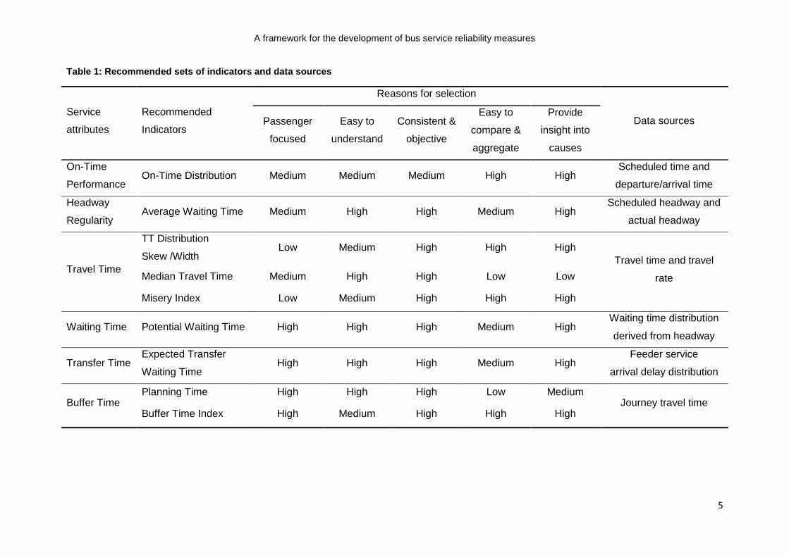
Abkowitz et al. (1978) evaluated the typical service reliability measures in an applied environment and selected several criteria, including explicitness of definition, controllability, expense and accurate measurability, and independenceCurrie et al. (2012) developed a framework to assess reliability indicators based on four criteria. Summarizing the evaluation criteria mentioned above, several key effective indicators are identified: (1) passenger focused; (2) easy to understand; (3) consistent and objective; (4) easy to compare and aggregate; and (5) insights into unreliability causes provided. The recommended sets of indicators and the reasons for their selection for different service attributes are listed in Table 2.


5

Table 1: Recommended sets of indicators and data sources

Service

attributes

Recommended

Indicators

Reasons for selection

Data sources Passenger

focused

Easy to

understand

Consistent &

objective

Easy to

compare &

aggregate

Provide

insight into

causes

On-Time

Performance On-Time Distribution Medium Medium Medium High High

Scheduled time and

departure/arrival time

Headway

Regularity Average Waiting Time Medium High High Medium High

Scheduled headway and

actual headway

Travel Time

TT Distribution

Skew /Width Low Medium High High High

Travel time and travel

rate Median Travel Time Medium High High Low Low

Misery Index Low Medium High High High

Waiting Time Potential Waiting Time High High High Medium High Waiting time distribution

derived from headway

Transfer Time Expected Transfer

Waiting Time High High High Medium High

Feeder service

arrival delay distribution

Buffer Time Planning Time High High High Low Medium

Journey travel time Buffer Time Index High Medium High High High

6

3 Framework for measurement development

Though buffer time is usually defined as buffer travel time, strictly speaking, buffer time should be recognized as an extreme value based concept to evaluate reliability performance. It can be applied manifoldly: (a) buffer waiting time to indicate budgeted waiting time needed to catch the expected bus; (b) buffer transfer time to indicate additional time required to avoid missed connections; and (c) buffer travel time to indicate extra time necessary for on time arrival. Analytical and empirical studies have confirmed buffer time as a powerful tool in indicating and estimating service reliability (Pu, 2011). Assuming there is no constraint on operating resources, buffer time based indicators could be viewed as the preferred choice for reflecting passenger-focused attributes.

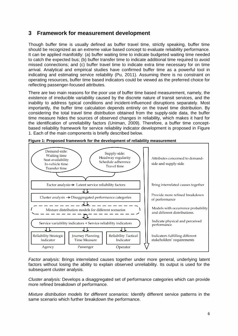
There are two main reasons for the poor use of buffer time based measurement, namely, the existence of irreducible variability caused by the discrete nature of transit services, and the inability to address typical conditions and incident-influenced disruptions separately. Most importantly, the buffer time calculation depends entirely on the travel time distribution. By considering the total travel time distribution obtained from the supply-side data, the buffer time measure hides the sources of observed changes in reliability, which makes it hard for the identification of unreliability factors (Uniman, 2009). Therefore, a buffer time concept-based reliability framework for service reliability indicator development is proposed in Figure 1. Each of the main components is briefly described below.

Figure 1: Proposed framework for the development of reliability measurement

Factor analysis: Brings interrelated causes together under more general, underlying latent factors without losing the ability to explain observed unreliability. Its output is used for the subsequent cluster analysis.

Cluster analysis: Develops a disaggregated set of performance categories which can provide more refined breakdown of performance.

Mixture distribution models for different scenarios: Identify different service patterns in the same scenario which further breakdown the performance.


7

Service variability and reliability indicators: Indicate what the service performance is and what the service is perceived to be.

Reliability strategic indicator: Useful for agencies to evaluate the value of time to make investment decisions. With the refined breakdown of performance, different values of buffer time can be given.

Journey planning time measure: provide passengers with departure time choice guaranteeing catching the expected bus, as well as their on-time arrival.

Reliability tactical indicator: provide operators with better insights into unreliability causes to implement effective measures to improve service performance. The framework is illustrated using bus travel time data from Brisbane, Australia in the next section.

4 Framework illustration

This section will use Automatic Vehicle Location (AVL) data to illustrate how the proposed framework works. AVL data were collected on a bus way section operating in Brisbane, Australia from 5:30am to 11:30pm for a two week period. The selected route was approximately 20 km long with 10 stops. Figure 2 illustrates the chosen transit service route. The travel time in this paper is based on the vehicle trips.

Figure 2: Concerned expressed bus transit route (from Google Map)

4.1 Data Cleaning

The archived data are screened to minimize the possibility that erroneous data would be used in further analyses. Two filters are used, namely erroneous trip and outlier. Erroneous trip filter excludes error trip records caused by incomplete trips, abnormal stops and hardware failures. Outlier filter screens the abnormal records caused by incidents. The Median Absolute Deviation (MAD) technique, also known as the Hampel Identifier, is applied for outlier identification. A sample is considered as an outlier if it is outside the range of the

8

lower bound value (LBV) and upper bound vale (UBV) determined by the MAD 3-delta criteria (Kieu et al., 2012).

Figure 3 displays the cleaning results for weekday inbound running time sample. The MAD cleaning technique seems to be promising with 3.2% outliers are identified. The oval-surrounded samples are far away from the normal pattern which could safely be treated as outliers and removed from the samples. However, the rectangle-surrounded samples cannot be regarded as outliers from the practical view. One of the main reasons for this is that the average sample size is too small for each 15 minutes time period (~ 9samples/period). Larger samples are needed to verify the effectiveness of the MAD cleaning technique.

After scrutinizing the cleaning outcomes, the distance between the outliers and their corresponding normal patterns are approximate 3~4 minutes which is a reasonable tolerant time in reality. Moreover, the outliers identified caused by incidents are still true trips samples and they should be taken into account in planning trips and assess service reliability performance. Therefore, all the samples presented in Figure 3 are used for further analysis.

Figure 3: Data cleaning results and outliers identified

4.2 Factor analysis

For the same service route line, the main factors causing unreliability are traffic demand and passenger volume. Conceptually, traffic demand and passenger volume may be described using dummy variables, namely time-of-day, day-of-week and operation direction (Kimpel, 2001). Factor analyses are needed to be taken to verify the correlations between the variables. The principle is like this, If the correlation between traffic demand and the dummy variables are high (such as, correlation index is larger than 0.85), then traffic demand can be substitute to dummy variables since they can contribute almost equally to the service variability while the dummy variables data are much easier to obtain in reality. As the lack of related dataset, this paper assumed the latent factors identified are time-of-day, day-of-week and operation directions. The latent factors are served as input to the cluster analysis in the next subsection.


9

4.3 Cluster analysis

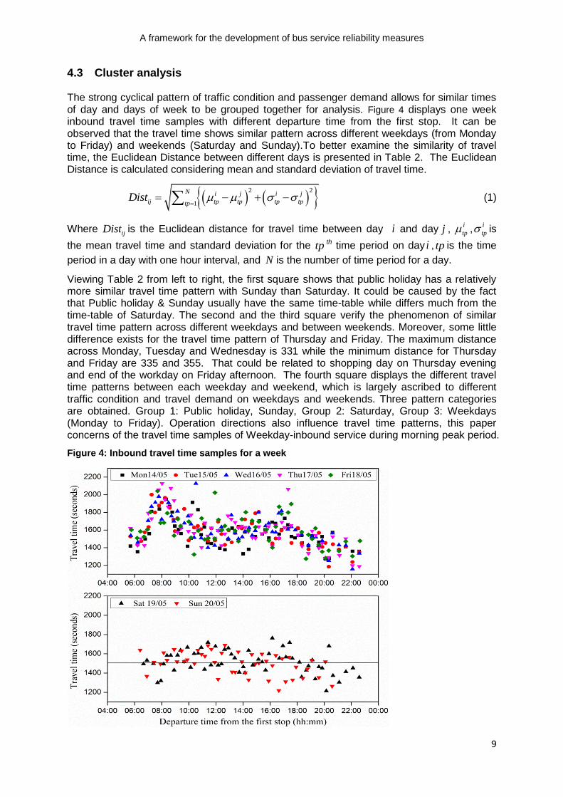
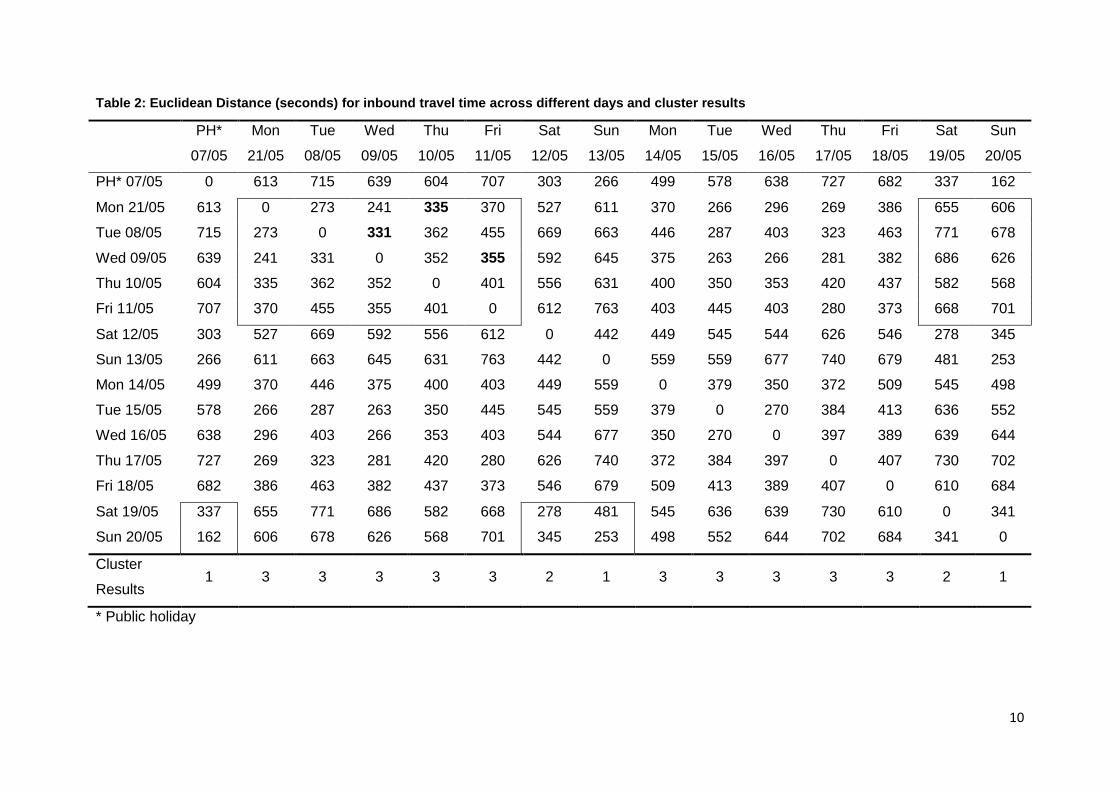
The strong cyclical pattern of traffic condition and passenger demand allows for similar times of day and days of week to be grouped together for analysis. Figure 4 displays one week inbound travel time samples with different departure time from the first stop. It can be observed that the travel time shows similar pattern across different weekdays (from Monday to Friday) and weekends (Saturday and Sunday).To better examine the similarity of travel time, the Euclidean Distance between different days is presented in Table 2. The Euclidean Distance is calculated considering mean and standard deviation of travel time.

2 2

1

N i j i j

ij tp tp tp tptpDist

(1)

Where ijDist is the Euclidean distance for travel time between day i and day j , i

tp ,i

tp is

the mean travel time and standard deviation for the tp th time period on day i , tp is the time

period in a day with one hour interval, and N is the number of time period for a day.

Viewing Table 2 from left to right, the first square shows that public holiday has a relatively more similar travel time pattern with Sunday than Saturday. It could be caused by the fact that Public holiday & Sunday usually have the same time-table while differs much from the time-table of Saturday. The second and the third square verify the phenomenon of similar travel time pattern across different weekdays and between weekends. Moreover, some little difference exists for the travel time pattern of Thursday and Friday. The maximum distance across Monday, Tuesday and Wednesday is 331 while the minimum distance for Thursday and Friday are 335 and 355. That could be related to shopping day on Thursday evening and end of the workday on Friday afternoon. The fourth square displays the different travel time patterns between each weekday and weekend, which is largely ascribed to different traffic condition and travel demand on weekdays and weekends. Three pattern categories are obtained. Group 1: Public holiday, Sunday, Group 2: Saturday, Group 3: Weekdays (Monday to Friday). Operation directions also influence travel time patterns, this paper concerns of the travel time samples of Weekday-inbound service during morning peak period.

Figure 4: Inbound travel time samples for a week

10

Table 2: Euclidean Distance (seconds) for inbound travel time across different days and cluster results

PH*

07/05

Mon

21/05

Tue

08/05

Wed

09/05

Thu

10/05

Fri

11/05

Sat

12/05

Sun

13/05

Mon

14/05

Tue

15/05

Wed

16/05

Thu

17/05

Fri

18/05

Sat

19/05

Sun

20/05

PH* 07/05 0 613 715 639 604 707 303 266 499 578 638 727 682 337 162

Mon 21/05 613 0 273 241 335 370 527 611 370 266 296 269 386 655 606

Tue 08/05 715 273 0 331 362 455 669 663 446 287 403 323 463 771 678

Wed 09/05 639 241 331 0 352 355 592 645 375 263 266 281 382 686 626

Thu 10/05 604 335 362 352 0 401 556 631 400 350 353 420 437 582 568

Fri 11/05 707 370 455 355 401 0 612 763 403 445 403 280 373 668 701

Sat 12/05 303 527 669 592 556 612 0 442 449 545 544 626 546 278 345

Sun 13/05 266 611 663 645 631 763 442 0 559 559 677 740 679 481 253

Mon 14/05 499 370 446 375 400 403 449 559 0 379 350 372 509 545 498

Tue 15/05 578 266 287 263 350 445 545 559 379 0 270 384 413 636 552

Wed 16/05 638 296 403 266 353 403 544 677 350 270 0 397 389 639 644

Thu 17/05 727 269 323 281 420 280 626 740 372 384 397 0 407 730 702

Fri 18/05 682 386 463 382 437 373 546 679 509 413 389 407 0 610 684

Sat 19/05 337 655 771 686 582 668 278 481 545 636 639 730 610 0 341

Sun 20/05 162 606 678 626 568 701 345 253 498 552 644 702 684 341 0

Cluster

Results 1 3 3 3 3 3 2 1 3 3 3 3 3 2 1

* Public holiday


11

4.4 Mixture travel time distribution modelling

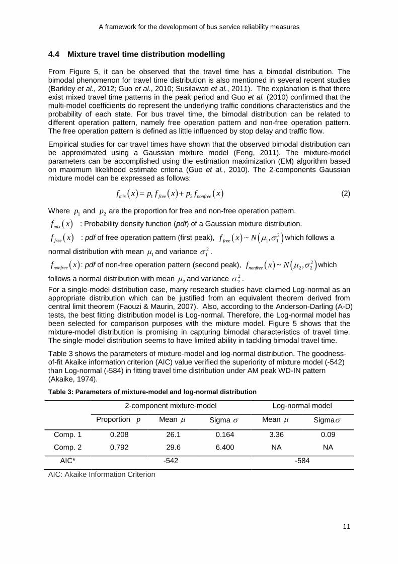
From Figure 5, it can be observed that the travel time has a bimodal distribution. The bimodal phenomenon for travel time distribution is also mentioned in several recent studies (Barkley et al., 2012; Guo et al., 2010; Susilawati et al., 2011). The explanation is that there exist mixed travel time patterns in the peak period and Guo et al. (2010) confirmed that the multi-model coefficients do represent the underlying traffic conditions characteristics and the probability of each state. For bus travel time, the bimodal distribution can be related to different operation pattern, namely free operation pattern and non-free operation pattern. The free operation pattern is defined as little influenced by stop delay and traffic flow.

Empirical studies for car travel times have shown that the observed bimodal distribution can be approximated using a Gaussian mixture model (Feng, 2011). The mixture-model parameters can be accomplished using the estimation maximization (EM) algorithm based on maximum likelihood estimate criteria (Guo et al., 2010). The 2-components Gaussian mixture model can be expressed as follows:

1 2mix free nonfreef x p f x p f x (2)

Where 1p and 2p are the proportion for free and non-free operation pattern.

mixf x : Probability density function (pdf) of a Gaussian mixture distribution.

freef x : pdf of free operation pattern (first peak), 2

1 1~ ,freef x N which follows a

normal distribution with mean 1 and variance 2

1 .

nonfreef x : pdf of non-free operation pattern (second peak), 2

2 2~ ,nonfreef x N which

follows a normal distribution with mean 2 and variance 2

2 .

For a single-model distribution case, many research studies have claimed Log-normal as an appropriate distribution which can be justified from an equivalent theorem derived from central limit theorem (Faouzi & Maurin, 2007). Also, according to the Anderson-Darling (A-D) tests, the best fitting distribution model is Log-normal. Therefore, the Log-normal model has been selected for comparison purposes with the mixture model. Figure 5 shows that the mixture-model distribution is promising in capturing bimodal characteristics of travel time. The single-model distribution seems to have limited ability in tackling bimodal travel time.

Table 3 shows the parameters of mixture-model and log-normal distribution. The goodness-of-fit Akaike information criterion (AIC) value verified the superiority of mixture model (-542) than Log-normal (-584) in fitting travel time distribution under AM peak WD-IN pattern (Akaike, 1974).

Table 3: Parameters of mixture-model and log-normal distribution

2-component mixture-model Log-normal model

Proportion p Mean Sigma Mean Sigma

Comp. 1 0.208 26.1 0.164 3.36 0.09

Comp. 2 0.792 29.6 6.400 NA NA

AIC* -542 -584

AIC: Akaike Information Criterion

12

Figure 5: PDF of travel time distribution fitted by mixture and individual models

4.5 Indicators for different stakeholders

Based on the proposed framework, three indicators for applications of reliability assessment (operators), journey planning (passenger) and value of time (agencies) are developed to fulfil different stakeholders’ requirements. The proposed indicators here only serve as examples and no quantification of the indicators is provided here. Detailed work can be referred to (MA et al., 2013).

Reliability tactical indicator: Operators are responsible for providing reliable operation service to the public. They are concerned of reliability assessment to gain deep insights into casual relationships between service inputs (service strategies) and outputs (reliability performance). The reliability tactical indicator is proposed as the expected reliability buffer time (ERBT) divided by the median travel time. The ERBT is defined as the expected value of reliability time under different operational patterns with consideration of travel time distribution.

1

N

i iiERBT p RBT

(3)

Where iRBT is reliability buffer time for state i , ip is proportion for state i , and N is the

state number. Reliability buffer time (RBT) is defined in the literature as the difference between xth percentile travel time (TTx) and yth percentile travel time (TTy). The selection of x and y depends on the study and usage purpose (Wakabayashi & Matsumoto, 2012).

Journey planning time: For public transport journey planning, passengers are concerned of deciding departure time to ensure an on-time arrival at their destinations. As Guo et al. (2010) stated, the reliability performance information reported to passengers can be like a weather report, such as the probability of encountering a non-free pattern during weekday peak periods is 80% and, if that happens, the additional buffer time to guarantee on time arrival is at least 12.8 minutes. Passengers can make their trip plans according to their trip’s purpose and their preferences. For a passenger who needs high reliability, he/she might choose additional time 12.8 minutes.

Value of reliability: Agencies are responsible for effective and efficient economic investment on public transport. They are concerned of quantify the value of reliability (VoR)


13

to better account for demand-side’s perception of reliability in the cost-benefit investment analysis. The generalized formula of the expected utility of reliability (in terms of time) can be written as follows (Carrion & Levinson, 2012).

_ _ _E U Expected Travel Time Expected Unreliability (4)

Where and are preference parameters that could be estimated from market survey.

Expected unreliability is defined as a function of reliability buffer time with considerations of different perceptions to importance of time.

1_

N

i i iiExpected Unreliability p RBT

(5)

Where i is the preference parameter for state i estimated from market survey.

The proposed measures take into account different perceived importance of time components under different operation states and the probability of states. The proposed expected reliability measure can indicate consistent reliability performance with a high resolution. The journey planning time can address different passengers’ departure choice for different trip purpose. The value of reliability measure is capable of reflecting passengers’ aversion to unreliability.

5 Conclusions

Improving service reliability is recognized as the most cost-effective approach to increase transit use by decreasing the perceived burdens of waiting at stops and longer travelling time en route. After reviewing current reliability measures, a general pool of indicators were summarized, from which a set of indicators can be selected for different objectives and operating constraints. Different sets of measures are recommended for different service attributes. Buffer time concept based indicators were discussed particularly.

A buffer time concept based framework is proposed for measurement development using AVL data. The framework can disaggregate service performance in a high level resolution and considers travel time distribution rather than only time points (e.g. planning time, median time). The framework working procedure is illustrated by means of AVL data from Brisbane. It can benefit public transport stakeholders in different ways, for instance, investment decisions for agencies, causes-effects analysis for operators and journey planning for passengers. This paper is the first step to investigate how the AVL data can be effectively used to measure service reliability. More work can be done along the same route as this research, such as, considering more service attributes to measure the expected unreliability (buffer waiting time, buffer transfer time, and seat availability).

6 Acknowledgments

The authors would like to thank the TransLink Division of Queensland DTMR (Department of Transport and Main Roads) for assistance with data collection. This work is supported by CSC (China Scholarship Council).

References

Abkowitz, M., Slavin, H., Waksman, R., Englisher, L., & Wilson, N. H. M. (1978). Transit service

reliability In TSC Urban and Regional Research Series. U.S. Department of Transportation

(DOT): Cambridge.

Akaike, H. (1974). A new look at the statistical model identification. Automatic Control, IEEE

Transactions on, 19(6), 716-723.

14

Barkley, T., Hranac, R., & Petty, K. (2012). Relating Travel Time Reliability and Nonrecurrent

Congestion with Multistate Models. Transportation Research Record: Journal of the

Transportation Research Board(2278), 13-20.

Bates, J., Polak, J., Jones, P., & Cook, A. (2001). The valuation of reliability for personal travel.

Transportation Research Part E: Logistics and Transportation Review, 37(2–3), 191-229.

Camus, R., Longo, G., & Macorini, C. (2005). Estimation of Transit Reliability Level-of-Service

Based on Automatic Vehicle Location Data. Transportation Research Record: Journal of the

Transportation Research Board, 1927(-1), 277-286.

Carrion, C., & Levinson, D. (2012). Value of travel time reliability: A review of current evidence.

[Review]. Transportation Research Part a-Policy and Practice, 46(4), 720-741.

Ceder, A. A. (2007). Public Transit Planning and Operation:Theory, modelling and practice: Elsevier

Ltd.

Currie, G., Douglas, N. J., & Kearns, I. (2012). An Assessment of Alternative Bus Reliability

Indicators Paper presented at the Australasian Transport Research Forum 2012 Proceedings,

Perth, Australia.

Fan, W. D., & Machemehl, R. B. (2009). Do transit ssers just wait for buses or wait with strategies.

Transportation Research Record: Journal of the Transportation Research Board, 2111(-1),

169-176.

Faouzi, N.-E. E., & Maurin, M. (2007). Reliability of travel time under lognormal distribution. Paper

presented at the Transport Research Board 86st Annual Meeting, Washington D.C.

Feng, Y. (2011). Arterial Travel Time Distribution Estimation and Applications. (Master of Science),

University of Minnesota.

Furth, P. G., & Muller, T. H. J. (2006). Service Reliability and Hidden Waiting Time: Insights from

Automatic Vehicle Location Data. Transportation Research Record: Journal of the

Transportation Research Board, 1955(-1), 79-87.

Furth, P. G., Muller, T. H. J., & Trb. (2006). Service reliability and hidden waiting time - Insights

from automatic vehicle location data. Paper presented at the 85th Annual Meeting of the

Transportation Research Board, Washington, DC

Golshani, F. (1983). System Regularity and Overtaking Rules in Bus Services. Journal of the

Operational Research Society, 591-597.

Goverde, R. M. P. (1999). Improving punctuality and transfer reliability by railway timetable

optimization. (Doctor of Philosopy ), Delft University of Technology.

Guo, F., Rakha, H., & Park, S. (2010). A Multi-State Travel Time Reliability Model. Paper presented

at the Transportation Research Board 89th Annual Meeting, Washington, DC.

Henderson, G., Adkins, H., & Kwong, P. (1991). Subway reliability and the odds of getting there on

time. Transportation Research Record, 1297(1297), 10–13.

Hollander, Y. (2006). The Cost of Bus Travel Time Variability. The University of Leeds.

Jang, W. (2010). Travel Time and Transfer Analysis Using Transit Smart Card Data. Transportation

Research Record: Journal of the Transportation Research Board, 2144(-1), 142-149.

Janos, M., & Furth, P. (2002). Bus Priority with Highly Interruptible Traffic Signal Control:

Simulation of San Juan's Avenida Ponce de Leon. Transportation Research Record: Journal

of the Transportation Research Board, 1811(-1), 157-165.

Kaparias, I., Bell, M. G. H., & Belzner, H. (2008). A new measure of travel time reliability for in-

vehicle navigation systems. Journal of Intelligent Transportation Systems, 12(4), 202-211.

Kieu, L., Bhaskar, A., & Chung, E. (2012). Bus and car travel time on urban networks: integrating

bluetooth and bus vehicle identification data. Paper presented at the ARRB Conference, 25th,

2012, Perth, Western Australia, Australia.

Kimpel, T. J. (2001). Time Point-Level Analysis of Transit Service Reliability and Passenger Demand.

(Doctor of Philosophy), Portland State University, Portland.

Kittelson & Associates, Urbitran, LKC Consulting Services, MORPACE International, Technology,

Q. U. o., & Nakanishi, Y. (2003). A Guidebook for Developing a Transit Performance-

Measurement System. Transport Research Board, Washington, D.C.

Lin, J., & Ruan, M. (2009). Probability-based bus headway regularity measure. Intelligent Transport

Systems, IET, 3(4), 400-408.


15

Liu, R., & Sinha, S. (2007). Modelling Urban Bus Service and Passenger Reliability. Paper presented

at the The Third International Symposium on Transportation Network Reliability, The Hague,

Netherlands.

Lomax, T., Schrank, D., Turner, S., & Margiotta, R. (2003). Selecting travel reliability measures.

Texas Transportation Institute monograph (May 2003).

MA, Z., Ferreira, L., & Mesbah, M. (2013). An alternative measure of bus service reliability at the

trip level. Submitted to Public Transport.

Mazloumi, E., Currie, G., & Rose, G. (2008). Causes of travel time unreliability–a Melbourne case

study. Paper presented at the 31st Australasian Transport Research Forum.

Meyer, M. D. (2002). Measuring system performance: Key to establishing operations as a core agency

mission. Transportation Research Record: Journal of the Transportation Research Board,

1817(-1), 155-162.

Nakanishi, Y. J. (1997). Bus Performance Indicators: On-Time Performance and Service Regularity.

Transportation Research Record: Journal of the Transportation Research Board, 1571(-1), 1-

13.

Osuna, E. E., & Newell, G. F. (1972). Control Strategies for an Idealized Public Transportation

System. Transportation Science, 6(1), 52.

Pronello, C., & Camusso, C. (2012). A Review of Transport Noise Indicators. Transport Reviews,

32(5), 599-628.

Pu, W. (2011). Analytic Relationships Between Travel Time Reliability Measures. Transportation

Research Record: Journal of the Transportation Research Board, 2254(-1), 122-130.

Pullen, W. T. (1993). Definition and measurement of quality of service for local public transport

management. Transport Reviews, 13(3), 247-264.

Shaw, T., & McLeod, D. (1998). Mobility performance measures handbook. Tallahassee, Florida,

Florida Department of Transportation, Systems Planning Office.

Strathman, J. G., Dueker, K. J., Kimpel, T., Gerhart, R., Turner, K., Taylor, P., . . . Hopper, J. (1999).

Automated bus dispatching, operations control, and service reliability: Baseline analysis.

Transportation Research Record(1666), 28-36.

Susilawati, S., Taylor, M. A., & Somenahalli, S. V. (2011). Distributions of travel time variability on

urban roads. Journal of Advanced Transportation.

Trompet, M., Liu, X., & Graham, D. (2011). Development of Key Performance Indicator to Compare

Regularity of Service Between Urban Bus Operators. Transportation Research Record:

Journal of the Transportation Research Board, 2216(-1), 33-41.

Turnquist, M. A., & Bowman, L. A. (1980). The effects of network structure on reliability of transit

service. Transportation Research Part B: Methodological, 14(1–2), 79-86.

Uniman, D. L. (2009). Service reliability measurement framework using smart card data: Application

to the london underground. (Master of Science), Massachusetts Institute of Technology.

van Lint, J., & van Zuylen, H. (2005). Monitoring and Predicting Freeway Travel Time Reliability:

Using Width and Skew of Day-to-Day Travel Time Distribution. Transportation Research

Record: Journal of the Transportation Research Board, 1917(-1), 54-62.

van Oort, N., & van Nes, R. (2004). Service Regularity Analysis for Urban Transit Network Design.

Paper presented at the Transportation Research Board 83st Annual Meeting

Wakabayashi, H., & Matsumoto, Y. (2012). Comparative study on travel time reliability indexes for

highway users and operators. [Article]. Journal of Advanced Transportation, 46(4), 318-339.

Yu, B., Yao, J., & Yang, Z. (2010). An improved headway-based holding strategy for bus transit.

Transportation Planning and Technology, 33(3), 329-341.

a framework for the development of bus service reliability...

Documents