ORIGINAL PAPER

A framework toward developing a groundwaterconceptual model

A. Izady & K. Davary & A. Alizadeh & A. N. Ziaei &A. Alipoor & A. Joodavi & M. L. Brusseau

Received: 12 February 2013 /Accepted: 3 May 2013# Saudi Society for Geosciences 2013

Abstract Developing an accurate conceptual model is themost important step in the process of a groundwater numericalmodeling. Disorganized and limited available data and infor-mation, especially in the developing countries, make the prep-aration of the conceptual model difficult and sometimescumbersome. In this research, an integrative and comprehen-sive method is proposed to develop groundwater conceptualmodel for an unconfined aquifer. The proposed method con-sists of six steps. A preliminary step (step 0) is aimed atcollecting all the available data and information. The outputof the first step as “controlling observations” is conceptualmodel version 00. This step should be rigorously checked dueto its critical role in the controlling of final conceptual model.Step 2 determines the aquifer geometry. The output of this stepis conceptual model version 01. Step 3 is responsible todetermine hydrodynamic properties and its output developsconceptual model version 02. Step 4 evaluates the surface andsubsurface interactions and lateral in/out groundwater flows.The output of this step is conceptual model version 03. Step 5is to integrate the results from other steps and to deliver thefinal conceptual model version. The accuracy level of theconceptual model and the annual groundwater balance isalso determined at this step. The presented groundwater con-ceptual model procedure was implemented for the Neishaboor

plain, Iran. Results showed its usefulness and practicality indeveloping the conceptual model for the study area.

Keywords Conceptual model . Groundwater .Development .

Iran

Introduction

Groundwater resources are considered to be significant andeconomical water resources. The comprehensive recognitionand proper utilization of this valuable resource, especially inarid and semi-arid areas, has an important influence on thesustainable development of social and economic activities(Izady et al. 2012). In the last decade, discords have occurredamong groundwater users for the rights of the groundwaterresource, particularly in highly exploited areas. The lack ofknowledge about the groundwater flow and the availability ofthe resource precluded the formulation of suitable groundwa-ter management plans (Nastev et al. 2005). Therefore, it isnecessary to simulate groundwater behavior for a better un-derstanding of the aquifer conditions. A simulation of ground-water behavior that takes into consideration the variousparameters and properties of aquifer is only possible throughmodeling (Bredehoeft and Hall 1995; Gerla and Matheney1996; Varni and Usunoff 1999; Nastev et al. 2005; Bedekar etal. 2012). In order to develop an appropriate numericalgroundwater flow model and a more quantitative representa-tion of the subsurface hydrology, the formation of a concep-tual model is critical (Vandenberg 1982; Neuman 1988;Anderson and Woessner 1992; EPA, DOE, NRC 1994;Reilly 2001; Neuman and Wierenga 2003a, b; Palma andBentley 2007; English et al. 2007; Barazzuoli et al. 2008;Seifert et al. 2008; Jusseret et al. 2009; Gillespie et al. 2012).The purpose of the conceptual model is to simplify the fieldproblem and organize the associated field data so that thesystem can be analyzed more readily by means of a numerical

A. Izady :K. Davary :A. Alizadeh :A. N. ZiaeiWater Engineering Department, College of Agriculture,Ferdowsi University of Mashhad, Mashhad, Iran

A. AlipoorNeishaboor Water Authority, Neishaboor, Iran

A. JoodaviEarth Sciences Department, College of Sciences,Shiraz University, Shiraz, Iran

A. Izady (*) :M. L. BrusseauSoil, Water and Environmental Science Department,University of Arizona, Tucson, AZ, USAe-mail: az.izady@gmail.com

Arab J GeosciDOI 10.1007/s12517-013-0971-9

model. A conceptual model is a pictorial representation of thegroundwater system in terms of hydrogeologic units, systemboundaries including time-varying inputs and outputs, andhydraulic as well as transport properties including their spatialvariability (Anderson and Woessner 1992; Meyer and Gee1999). The conceptual model is the basic idea of how thesystem or process operates; it forms the basic idea for themodel (Bredehoeft 2005). Conceptual models are built on thepast experience or previous work in a study area, knowledgeof similar hydrogeologic regimes, site-specific data, and eveninstitutional paradigms (Gillespie et al. 2012). In fact, onespecific but very important component of the modeling pro-cess is the conceptualization of actual groundwater system.Also, it has been suggested that uncertainty in groundwatermodeling is largely dominated by uncertainties arising fromthe definition of groundwater conceptual models (Carrera andNeuman 1986a, b; Neuman and Wierenga 2003a, b; Højbergand Refsgaard 2005; Poeter and Anderson 2005; Refsgaard etal. 2006; Meyer et al. 2007; Ye et al. 2010; Rojas et al. 2008,2010a, b). In recent years, a number of authors have acknowl-edged that conceptual model uncertainty which has receivedless formal attention in groundwater applications than itshould (Neuman 2003; Neuman and Wierenga 2003a, b;Bredehoeft 2003, 2005; Carrera et al. 2005; Poeter andAnderson 2005; Refsgaard et al. 2006; Rojas et al. 2008).Moreover, ignoring conceptual model uncertainty may resultin biased predictions and/or underestimation of predictiveuncertainty (Ye et al. 2010).

Despite the utmost importance of the groundwater concep-tual model, not much of detailed instructions or procedures areavailable to build up such a model; however, some generalguidelines have been published (Anderson’s book; Andersonand Woessner 1992, USGS reports). Moreover, disorganizedand limited available data and information, especially in thedeveloping countries, make the conceptual modeling com-plicated and tedious. Therefore, in this research a newdetailed procedure was presented to develop a groundwaterconceptual model for an unconfined aquifer. Additionally,the proposed method has been applied, to confirm andprove the suitability and applicability of the suggestedapproach, to the Neishaboor plain.

Materials and methods

The study area

Neishaboor watershed is located between 35° 40′N to 36° 39′N latitude and 58° 17′ E to 59° 30′ E longitude with semi-aridto arid climate, in the northeast of Iran (Fig. 1). The totalgeographical area is 9,158 km2 that consists of 4,241 km2

mountainous terrains and about 4,917 km2 plain. The maxi-mum elevation is located in the BinaloodMountains (3,300 m

above sea level), and the minimum elevation is at the outlet ofthe watershed (Hoseinabad) at 1,050 m above sea level. Theaverage daily discharge at Hoseinabad hydrometric stationwas 0.36m3 s−1 for the period of 1997–2010, with a minimumvalue of zero and a maximum value of 89 m3 s−1. The averageannual precipitation is 265 mm, but this varies considerablyfrom one year to another (CV=0.13). The mean annual tem-peratures changes from 13 °C at Bar station (in the mountain-ous area) to 13.8 °C at Fedisheh station (in the plain area). Theannual potential evapotranspiration is about 2,335 mm(Velayati and Tavassloi 1991).

Neishaboor watershed is located between Binalood andCentral Iran structural zones, and is separated into twodistinct parts from a geological viewpoint (Fig. 1). Themountainous northeast part of the watershed consists ofDevonian and Silurian calcareous and dolomitic formations,Jurassic siltstone, and calcareous rocks in the vicinity ofEocene and Neogene clastic sediments. The second part,which is located in southeast, south, and west mountainousparts of the study area, comprise Upper Cretaceousophiolites (southwest and west) and volcanic rocks. Thelargest riparian trace is located in Maroosk river approxi-mately 500 m in width. The major alluvium plans of studyarea are located at south of Kharv (the area is approximately36 km2). Moreover, there are several alluvium plans locatedin Mirabad area (north of Neishaboor city) with the wholearea of about 27 km2. Furthermore, alluvium plains can beseen in the north of the study area (such as Bujan, Grineh,Maroosk, etc.) which the area is about 40 to 50 km2. Inaddition, medium grain size alluviums with fine matrixcover an extensive part of the Neishaboor plain. Limonand argil fine-grain-size alluviums cover the central partsof the study plain. These fine-grained alluviums had becomesaline near to the plain’s outlet due to evaporation fromgroundwater in the past (Velayati and Tavassloi 1991).

Theoretical background of the proposed procedure

A conceptual model of groundwater flow is an aggregatedand qualitative framework upon which data related to sub-surface hydrology can be interpreted (Anderson andWoessner 1992; Reilly 2001; Neuman and Wierenga2003a, b; Palma and Bentley 2007; English et al. 2007;Barazzuoli et al. 2008; Jusseret et al. 2009). Developmentof the conceptual model requires a rigorous and conscien-tious incorporation of data, information, and reportspertaining to the aquifer and groundwater flow in the projectarea. The basic components of a groundwater conceptualmodel are physical boundaries and appropriate boundaryconditions, distribution of hydrodynamic properties, andsurface and subsurface interactions. A conceptual modelcan subsequently be populated with project-specific charac-teristics, such as groundwater levels, recharge zones, and

Arab J Geosci

connectivity between withdrawal points and dischargezones, and finally will be used for numerical modeling.

The conceptual model also allows the general conclusionsregarding the impacts of hydrologic conditions on groundwater

Fig. 1 a Neishaboor watershed location map. b Sedimentary and struc-tural zones of Iran. c Geological map along with main aquifer, meteoro-logical stations, and river network of the Neishaboor watershed. Note that

NM, Ng cs, Qal, Qc, Qt1, and Qt2 are marl, red-brown, and gypsiferous;siltstone; sandstone; conglomerate; recent alluvium; clay flat; olderterraces; and younger gravel fans and terraces, respectively

Arab J Geosci

flow. Moreover, conceptualization is useful to explore hid-den facts and to fill data gaps for a better understanding ofthe groundwater system. Undoubtedly, accuracy level of thenumerical model inversely depends on the depth of thesegaps (data uncertainty, data scarcity, etc.). Therefore, aconceptual model evolves forever and conceptualization isan endless process. Figure 2 shows an overall schematicdiagram of the suggested “conceptual model development”procedure.

Figure 2 shows a six-step procedure (0 to 5) for developinga groundwater conceptual model. The preliminary step isaimed at collection of all available quantitative and qualitativedata and information. Step 1 is the very basic step that controlsother steps. In fact, information from observation wells,hydrometric stations, and withdrawal wells’ discharges arechosen as “controlling observations”. However, to makesure these data are adequately confident and flawless, theyare double-checked against each other and any other factualdata rigorously. Any remaining persistent conflictingdata/information is omitted from the controlling data set.Step 2 is to determine the aquifer geometry. One of theinfluential data for this step is digital elevation model(DEM). The bedrock position, aquifer physical boundary,and stratigraphy of the aquifer are determined at this stage.Before entering the next step, a consistency evaluation (CE)in regards to controlling observations has to be done. If anyinconsistency (or conflict) is found, then step 2 isreconsidered to resolve the conflicts. Step 3 is responsible

to determine the hydrodynamic properties of the aquifer.Again a CE has to be done, but these time outputs ofstep 2 are added to the controlling data set. If any incon-sistency (or conflict) is found, then steps 2 and 3 arereconsidered to resolve the conflict. Step 4 is aimed atevaluation of the interaction between surface water andgroundwater bodies. Also, this step determines anyincoming/outgoing groundwater flows between the aquiferand its surroundings. At this stage, CE is also necessary. Ifany inconsistency (or conflict) is found, then steps 3 and 4are reconsidered to resolve the conflict. The last step, step5, is to integrate the results from other steps to deliver theoverall conceptual model and estimate the annual ground-water balance components. At this stage, based on theadequacy/accuracy of the available data/information, theaccuracy level of the conceptual model is determined.This is done for each parameter separately via scoringspatial availability of measured or estimated data and therobustness of estimated data. Moreover, adequacy of con-ceptual model is elaborated to serve a numerical model.Upon the results of the last step, a list of furtherstudies/tests has to be recommended to fill the gaps andpromote the model accuracy that enhances the aquiferconceptualization. If development of a satisfactory numeri-cal model is required, the list should contain minimumprerequisites of the numerical model. However, a compre-hensive list would be generated with respect to the concep-tual model accuracy level.

Fig. 2 Schematic diagram ofthe development procedure forthe groundwater conceptualmodel. CE is the acronym forconsistency evaluation. Itmeans that if any inconsistency(or conflict) is found among thespecified steps, those arere-considered to resolve theconflict with regards tocontrolling observations

Arab J Geosci

Worth to be mentioned is the hierarchy of reference to theinformation. We considered available data/information in threelevels: quantitative observed data, qualitative observed data, andlocal expert experiences. In each step, main data/information(quantitative and qualitative observed data) is to be conferredfirstly. Next, if the spatial distribution (abundance/scarcity) isnot satisfactory, then one has to refer to the third-level data.Keep in mind that usage of the third-level data must be mini-mized due to their inherent ambiguity and uncertainty. This hasconcluded to a “satisfied with…” check within steps, as shownin steps flowcharts. Note that minimum usage of the third-leveldata is limited to enhancement of spatial distribution ofdata, while in the case of conceptual model conflicts(conflict between steps) all available data must be used.

Pre-step (step 0): Collect all available data and informationAt the pre-step, all available data and information

(quantitative or qualitative) are summed up. It isstrongly recommended to collect all data and infor-mation from all available sources. Particularly, in thedeveloping countries which suffer from disorganizeddata sources, more attempts should be made. Thelocal expert knowledge is a crucial qualitative sourceof information in such circumstances.

Step 1: Set up controlling observationsStep 1 is a basic step that controls other steps

(Fig. 3). The information and data from piezometers,hydrometric stations, and discharges from with-drawal wells are chosen as “controlling observa-tions”. In fact, these precious data and informationhave an important role to develop a conceptualmodel. Therefore, these should be cross-checkedagainst each other and any other factual data to makesure that the data is adequately confident and flaw-less. For example, groundwater level in piezometers

is investigated whether it represents a deep or aperched aquifer water table. For this reason, thecomparison of mentioned groundwater level withdepth of groundwater in other surrounding wellswould be useful. Also, hydrometric data is used toapproximate groundwater contribution (baseflow) tosurface flows. If there was any persistent conflictingdata/information, they should be omitted from thecontrolling data set due to its great importance inother steps of developing groundwater conceptualmodel. However, it is sturdily advised to keep allavailable data. The output of this step is concep-tual model version (ver.) 00 as both maps andtime series tables.

Step 2: Situate aquifer geometryStep 2 determines the aquifer geometry. The

first output of this step is ground surface DEMand aquifer physical boundary; bedrock and stra-tigraphy of the aquifer are then defined at thisstage. Figure 4 shows a schematic diagram of step2 and its output.

Surface topography validation

Basic topographic attributes extracted fromDEMare entered tothe groundwater models. The alluvium and saturated layerthicknesses are directly affected by the accuracy of the selectedDEM. Thus, it is strongly recommended that the accuracy ofavailable DEMs be examined before being approved. Theterrain elevation data are accessible from several major sourceswith low to high spatial resolutions. These are mainly localtopographicmaps, Shuttle Radar TopographyMission (SRTM)(http://srtm.csi.cgiar.org/SELECTION/inputCoord.asp) andAdvanced Space-borne Thermal Emission and Reflection

Fig. 3 Schematic diagram ofstep 1 and its output

Arab J Geosci

Radiometer (ASTER) (http://www.gdem.aster.ersdac.or.jp/search.jsp). The ground surface level at the piezometer loca-tions can be used as a benchmark to check the accuracy of theavailable DEMs. Field measurements with deferential GPStechnique is also recommended for checking these DEMsagainst each other and for conflicting points.

Aquifer physical boundary

The physical limits of the study region must be determined todevelop any groundwater conceptual model. Figure 5 shows aschematic diagram of the required steps for this process.

Topography and geology maps are used to make a firstdraft of the aquifer physical boundary. This boundary is thenamended using intersection points of current groundwaterlevel and bedrock maps to produce a preliminary physicalboundary map. At this stage, many boundary points need tobe modified due to an ambiguity of the groundwater tablenear boundary. For this reason, bedrock and groundwaterlevel raster layers are subtracted from each other. In theobtained raster layer, wherever the bedrock located abovethe groundwater level, the boundary should be manuallycorrected. This is done based on local expert knowledge,and depth and discharge of withdrawal wells.

Bedrock position

The bedrock is known as a lower boundary of an aquifer.Figure 6 shows a schematic diagram of required steps fordetermination of the bedrock.

Usually, borehole logs together with geo-electric soundingmeasurements (interpreted using general geological andhydrogeological information) are used to determine theposition of the bedrock. However, this information isnot sufficient in many locations and still there areambiguities with the bedrock positioning. Therefore,other information such as logs from any fully penetratedwithdrawal wells, is useful to clarify the bedrock posi-tion. Many more cross-checks should be made betweenthese results and other information such as local expertknowledge and even experiences/observations of well-drillers teams.

Aquifer stratigraphy

Aquifers can be generally categorized to unconfined, semi-confined, and confined. The aquifer type is often derivedfrom geo-electric soundings results, pumping tests, dril-ling logs, and local expert knowledge. This process iscommonly called stratigraphy which specifies the aqui-fer heterogeneity and anisotropy. In general, the detailsof this process follow the same paths as the process ofbedrock determination.

CE1 Before entering step 3, findings of this step have to bechecked with “controlling observations” step (step 1).Specifically, elevations of bedrock and withdrawal wellsbottoms are to be checked against each other. If any with-drawal well has penetrated through the bedrock, this is thenconsidered as a potential conflict that has to be resolved.

Fig. 4 Schematic diagram ofstep 2 and its output

Arab J Geosci

Step 3: Estimation of hydrodynamic propertiesIn this step, the spatial distribution of the

aquifer hydrodynamic properties are estimated(Fig. 7).

Hydraulic conductivity

The spatial distribution of the hydraulic conductivity is oneof the most challenging aspects of hydrogeology modeling.

Fig. 5 Schematic diagram of required steps for determination of the physical boundary

Arab J Geosci

Fig. 6 Schematic diagram of required steps for determination of the bedrock

Arab J Geosci

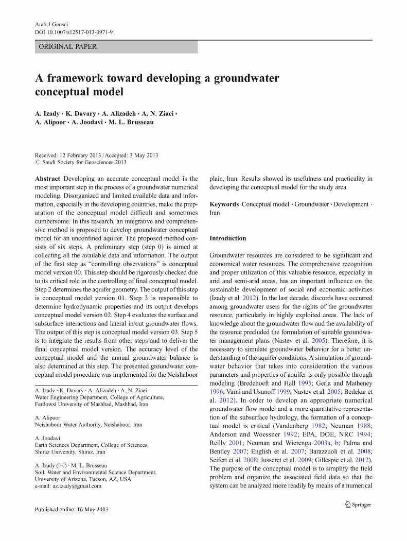
The aquifer heterogeneity not only influences the ground-water flow but also has the greatest impacts on the move-ment of contaminants. It has been shown that the spatialdistribution of hydraulic conductivity forms a large sourceof uncertainty in groundwater modeling (Freeze 1975;Gelhar 1986; Moore and Doherty 2005; Rojas et al.2010a, b). Usually, the spatial distribution of the measuredhydraulic conductivities is not sufficient for the groundwatermodel calibration. Therefore, appropriate estimation of thehydraulic conductivity has an undeniable role in groundwatermodeling. Figure 8 shows a schematic diagram of requiredsteps for determination of the hydraulic conductivity.

There are direct and indirect methods to estimate saturatedhydraulic conductivity (Ks). The direct methods (e.g., pumpingtest, tracer test, etc.) are based on field measurements ofsaturated hydraulic conductivity or transmissivity to generaterealizations of the Ks or T (Hill et al. 1998; Moore and Doherty2005). However, the measurement of Ks in the field is costly,time consuming, and cumbersome.

Additionally, the aquifer heterogeneity implies a largenumber of field measurements to characterize the horizontaland vertical hydraulic conductivity of the study area (Jabro1992). Accurate estimation of Ks in the field is limited bythe lack of precise knowledge of the aquifer heterogeneity(Uma et al. 1989). Therefore, it is necessary to apply sim-plified empirical methods to estimate the saturated hydraulicconductivity based on easily measurable aquifer properties.Particularly, hydrogeologists have attempted to relatehydraulic conductivity to grain size (Egboka and Uma1986; Uma et al. 1989; Pinder and Celia 2006). Therelationship between specific yield and hydraulic con-ductivity can also be used to estimate these parametersbased on which one is available (Theis et al. 1963;Lohman 1972; Ahuja et al. 1989; Razack and Huntley 1991;Hamm et al. 2005). In other words, the specific yield data

obtained from well development reports and other resourcescan provide useful estimates of hydraulic conductivity. Thegeo-electric method is also used to estimate hydraulic con-ductivity based on transverse resistance (Griffith 1976; Kelly1977; Louis et al. 2004).

Keeping in mind that estimated hydraulic conductivityshould be amended with other geological facts such asformation types and saturated and alluvium thickness, espe-cially where a falling water table exists, old measured Kvalues have to be revised.

Specific yield

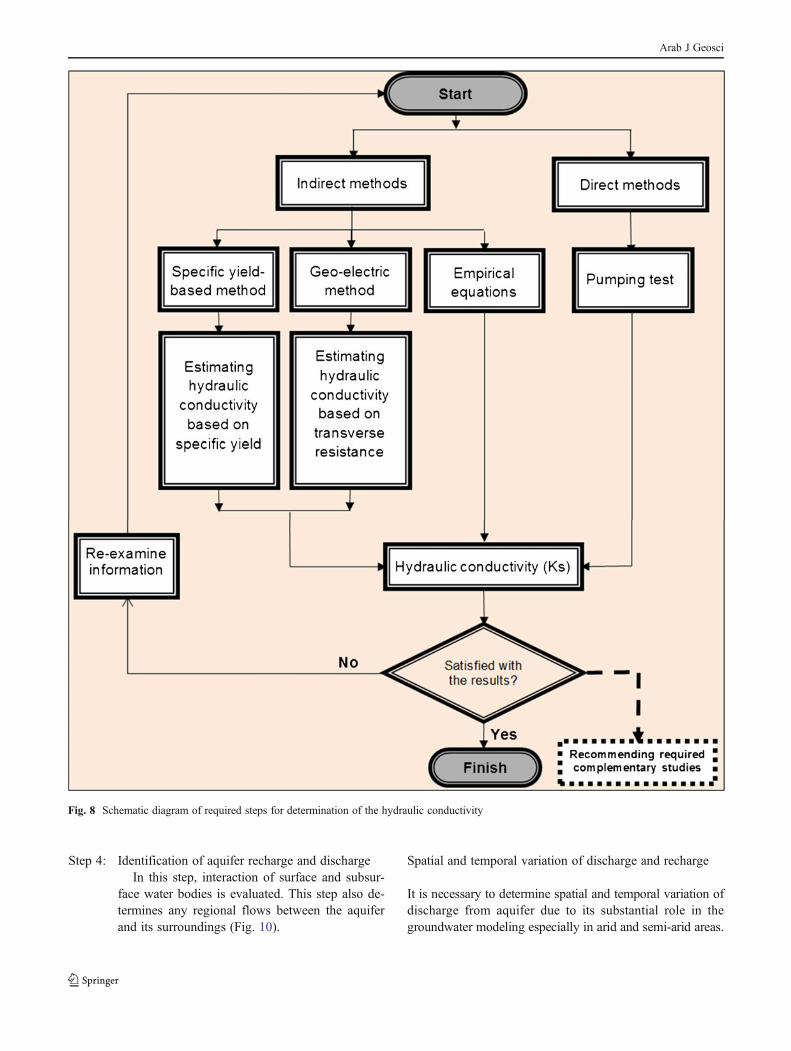
Beside to hydraulic conductivity, the specific yield has acrucial effect on the accuracy of groundwater modeling.Existence of reliable specific yield estimations facilitatesthe model calibration. Figure 9 illustrates the required stepsfor estimating the specific yield.

There are direct and indirect methods to estimate specificyield. Most of the details of this process follow same pathsas the process of hydraulic conductivity estimation; there-fore, the granulation method is only reported here (Johnson1967). In this method, the texture of the excavated materialsfrom different depths are determined, and based on theirtexture, the specific yield of the materials are estimated fromthe typical tables such as Table 1. The weighted averageof the estimated specific yields can be designated as thespecific yield of the aquifer in the spot of excavation.In the presence of a falling water table, old measuredspecific yields should be corrected.

CE2 Before entering step 4, findings of this step have to bechecked with those of steps 1 and 2. Specifically, estimatedKs and Sy values have to be consistent with wells’ saturateddepths and discharges.

Fig. 7 Schematic diagram ofstep 3 and its output

Arab J Geosci

Step 4: Identification of aquifer recharge and dischargeIn this step, interaction of surface and subsur-

face water bodies is evaluated. This step also de-termines any regional flows between the aquiferand its surroundings (Fig. 10).

Spatial and temporal variation of discharge and recharge

It is necessary to determine spatial and temporal variation ofdischarge from aquifer due to its substantial role in thegroundwater modeling especially in arid and semi-arid areas.

Fig. 8 Schematic diagram of required steps for determination of the hydraulic conductivity

Arab J Geosci

The discharge temporal variation of each withdrawal wellshould be specified. Discharge data in many developing coun-tries are usually measured every few years (i.e., samplinginterval, say 5-year). Care has to be given not to mismatchwithdrawal wells records from one sampling to another.

Knowing discharges of each withdrawal well, for twoconsecutive discharge sampling years, a linear variationis considered to define the discharge trend.

It seems that the quantification of groundwater rechargeis a major problem in many water-resource investigations.

Fig. 9 Schematic diagram of required steps for determination of specific yield

Arab J Geosci

This is particularly intensified in arid and semi-arid areas,with very small recharge quantities, where small groundwa-ter recharges are likely to be lost in the uncertainty of thedominant larger inputs and outputs (Allison et al. 1984;Gieske 1992; Wheater 2010). It is believed that rechargetakes place through four pathways: through fractured rocksin the mountain block with subsequent flow to aquifers, inalluvial fans at the base of the mountains, within stream-beds, and direct infiltration in the plain.

Mountain block recharge is difficult to assess due to itsinherent uncertainty. Mountain front recharge can be assessedusing traditional methods based on piezometers, if available.Recharge from alluvial fan is the most important rechargecomponent in arid and semi-arid areas. Piezometers are alsoused tomeasure the recharge from alluvial fans. In the absence

of such data, the boundary of aquifer has to be shifted inwardto the first available piezometer. Then, the recharge fromalluvial fan becomes a regional /lateral recharge. Streambedrecharge is discussed in the next section.

A wide variety of methods is available to estimate directinfiltration from plain. Determining which of these techniquesis likely to provide reliable recharge estimates is often difficult.Various factors need to be considered when choosing a methodof quantifying recharge (precipitation, evapotranspiration, soil,land use, and crop management). A thorough understanding ofthe attributes of the different techniques is critical. Literaturereview shows that among all methods for estimating recharge,models play a very useful role in the recharge estimationprocess (Scanlon et al. 2002). They are used to determinesensitivity of recharge estimates to various parameters andto predict how future changes in climate and land use mayaffect recharge rates. The water balance methods such asWTF (water table fluctuation) (Meinzer 1923; Meinzer andStearns 1929), CRD (cumulative rainfall departure)(Bredenkamp et al. 1995), and RIB (rainfall infiltrationbreakthrough) (Xu and Beekman 2003) can also be used,provided that reliable water table data is available. However,to develop the conceptual model a simple and applicablemethod with acceptable accuracy is to estimate rechargeaccording to groundwater transmissivity (Gieske 1992;Dewandel et al. 2008; Wheater 2010). In this method,aquifer is divided into several zones based on its transmis-sivity. The recharge was then estimated as a percentage ofeffective precipitation (Gieske 1992; Wheater 2010) andgroundwater extraction (Dewandel et al. 2008) for differentzones. Additionally, a percentage of potential evaporation isconsidered as groundwater evaporation from the water table,if the depth of groundwater is less than 5 m. Figure 11

Table 1 Specific yield in percent for different soil textures and mate-rials (after Johnson 1967)

Material Specific yield (%)

Maximum Minimum Average

Clay 5 0 2

Sandy clay 12 3 7

Silt 19 3 18

Fine sand 28 10 21

Medium sand 32 15 26

Coarse sand 35 20 27

Gravelly sand 35 20 25

Fine gravel 35 21 25

Medium gravel 26 13 23

Coarse gravel 26 12 22

Fig. 10 Schematic diagram ofstep 4 and its output

Arab J Geosci

shows a schematic diagram of required steps for estimationof direct recharge from plain based on transmissivity.

Interaction between groundwater and surface water

Accurate representation of groundwater–surface water interac-tions is crucial for groundwater modeling in the arid and semi-arid areas. In fact, groundwater and surface water are notisolated components of the hydrologic system but instead in-teract in a variety of aspects. Therefore, an understanding of thebasic principles of interactions between groundwater and sur-face water is needed for effective management of groundwaterresources. A more detailed description of the groundwater–surface water interactions is given by Sophocleous (2002). Inmany arid/semi-arid areas with a thick vadose zone, the inter-action is mostly a recharge from streams to aquifer. Streambed

recharge can be estimated using the water balance model.Although it is relatively simple to estimate, streambed rechargeis still poorly characterized. The easiest approach to measuringstreambed recharge is through measurement of channel lossesthrough channel path. This requires that the flow bemeasured atseveral locations along a stream within the flow period.Excluding withdrawals, any downstream decrease in flow isattributed to recharge through the bed between the measure-ments locations. While conceptually simple and requiring min-imal instrumentation, this approach needs hydrometric stations;otherwise, it is costly and time consuming.

Boundary condition

Groundwater flow models typically have upper, lateral, andlower boundaries. The upper boundary is often taken to be

Fig. 11 Schematic diagram of required steps for direct recharge estimation based on transmissivity

Arab J Geosci

the groundwater levels. Piezometer water levels are usuallygiven as initial condition. The lower boundary of a model isoften considered to be the bedrock (explained in the “TheBedrock” section). The lateral boundaries are often the mostdifficult to be defined for hydrologic analysis. These bound-aries are characterized as one of three types. For the firsttype, the groundwater level at the boundary is defined as afunction of time. For the second type, the flux of wateracross the boundary is defined as a function of time. Forthe third boundary type, a no-flow boundary is assigned.The groundwater levels along with geo-electric measure-ments in the boundaries are analyzed with flownet techniqueto determine the boundary types (Anderson and Woessner1992). Local expert knowledge is undoubtedly useful forenhancement of the conceptual model.

CE3 Before entering step 5, findings of this step have to bechecked within and between. The within check is to makesure that the results are rational due to the aquifer annualwater balance. The between check is made of many folds.The recharge amounts and seasonalities have to be consistentwith the aquifer thickness, water-table elevations and itsseasonalities, and also land use. The lateral boundary condi-tions have to be consistent with surrounding geological fea-tures, as well as with granulation and groundwater gradients.

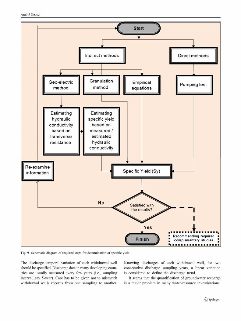
Step 5: Deliver final version of the conceptual modelStep 5 is to integrate the results from other steps

and to determine spatial accuracy level of theconceptual model components. Main outputs ofthis step are declaration of mathematical modelingfeasibility and the annual groundwater balance(Fig. 12).

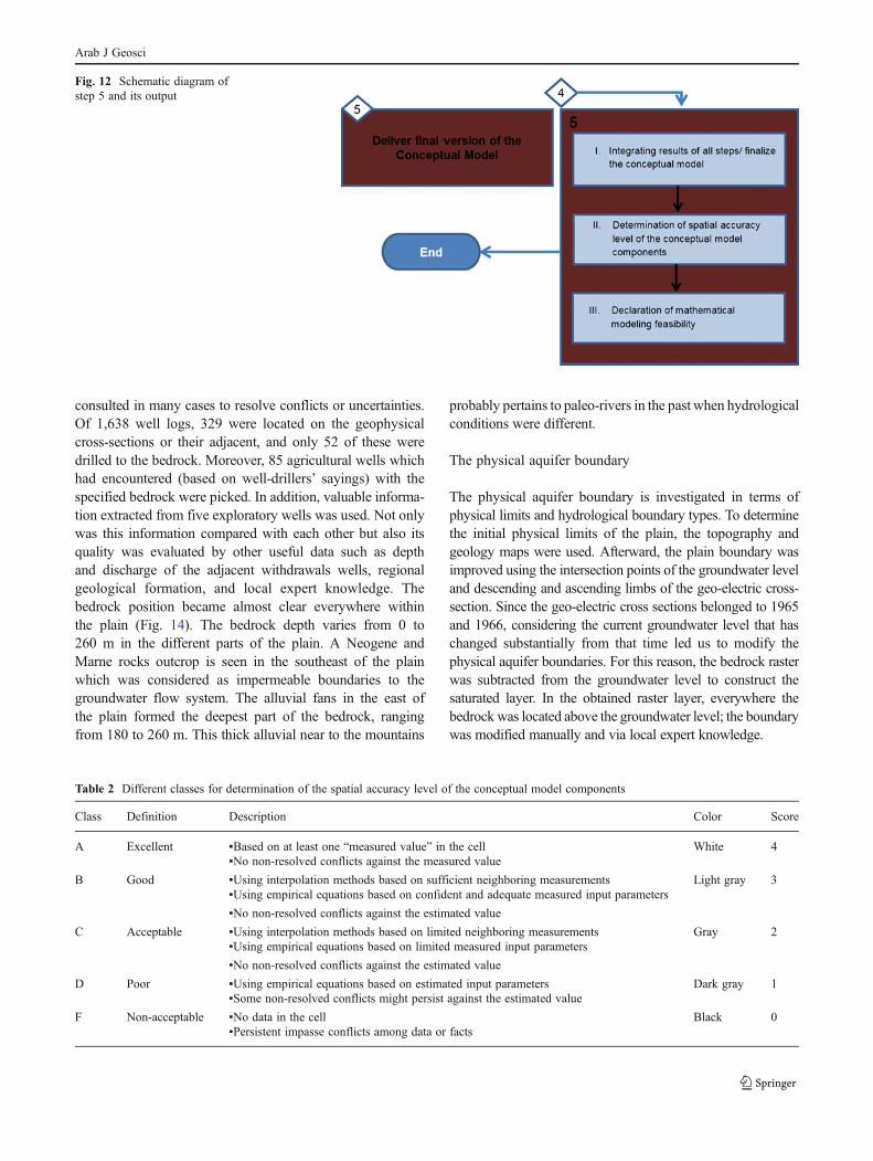
To visualize the accuracy of the developed con-ceptual model, a grid with proper cell size (com-pared to the plain area) is overlaid on the aquifermap. Then, the spatial accuracy level for eachcomponent of the conceptual model is specifiedfor all grid cells, in five different classes, asexplained in Table 2.

The ultimate score of each grid cell is summedup based on the score of the conceptual modelcomponents. The overall accuracy of the concep-tual model is then summarized via average cells’scores. At this stage and based on determinedaccuracy level, feasibility of aquifer mathematicalmodeling should be assessed. Surely, this is rele-vant to desired accuracy and is judgmental.Another issue at this stage is to determine theminimum required gap filling complementarystudies. This is to enhance the conceptual modelaccuracy to a satisfactory level for mathematicalmodeling. The final conceptual model is only

revisited when sufficient up-to-date data havebeen collected, which often may take severalyears, or when new information and/or scientificevidence challenge the original conceptualiza-tion. It is worthy to be reminded that the con-ceptual model is not only a prerequisite formodeling but is also the base of any managerialdecision making.

Application of proposed method in the Neishaboor plain

Results of the developed conceptual model for the Neishabooraquifer are presented in the following sections.

Hydraulic heads (controlling observations)

The groundwater elevations from piezometers were checkedfor their veracity in this step. The interpolated potentiomet-ric surface, based on groundwater level measurements, isshown in Fig. 13. The regional groundwater flow originatesprimarily from the east, northeast, and south, and dischargesto the southwest of the study area.

Aquifer geometry

The terrain surface

Among available topographic maps, two with 1/50,000and 1/25,000 scales were selected. Moreover, SRTMand ASTER DEMs were downloaded. These werecross-checked against each other and for conflictingpoints a field measurement of the piezometer coordi-nates and the ground surface elevation at these pointswith deferential GPS technique was performed. Thepiezometers (official elevations) were considered asbenchmark points. The investigation shows these bench-marks are best matched with SRTM DEM (RMSE was8.82, 5.12, 4.33, and 9.44 m for 1/50,000, 1/25,000,SRTM, and ASTER DEMs, respectively). Finally,SRTM DEM was selected as the base elevation model.

The bedrock

To determine the position of the bedrock, the geo-electricsounding results from 1965 and 1966 (in 21 cross-sections,with 232 sounding points) were used. The distribution of thesegeo-electric soundings was satisfactory. Through the recentyears, much new valuable information has been added. Toachieve maximum possible clarity for the bedrock, a combi-nation of old and new information was considered. Newinformation consisted of withdrawal well logs, scattered geo-electric soundings (49 case, for other applications), and newborehole logs. Besides, local experts and/or drillers were

Arab J Geosci

consulted in many cases to resolve conflicts or uncertainties.Of 1,638 well logs, 329 were located on the geophysicalcross-sections or their adjacent, and only 52 of these weredrilled to the bedrock. Moreover, 85 agricultural wells whichhad encountered (based on well-drillers’ sayings) with thespecified bedrock were picked. In addition, valuable informa-tion extracted from five exploratory wells was used. Not onlywas this information compared with each other but also itsquality was evaluated by other useful data such as depthand discharge of the adjacent withdrawals wells, regionalgeological formation, and local expert knowledge. Thebedrock position became almost clear everywhere withinthe plain (Fig. 14). The bedrock depth varies from 0 to260 m in the different parts of the plain. A Neogene andMarne rocks outcrop is seen in the southeast of the plainwhich was considered as impermeable boundaries to thegroundwater flow system. The alluvial fans in the east ofthe plain formed the deepest part of the bedrock, rangingfrom 180 to 260 m. This thick alluvial near to the mountains

probably pertains to paleo-rivers in the past when hydrologicalconditions were different.

The physical aquifer boundary

The physical aquifer boundary is investigated in terms ofphysical limits and hydrological boundary types. To determinethe initial physical limits of the plain, the topography andgeology maps were used. Afterward, the plain boundary wasimproved using the intersection points of the groundwater leveland descending and ascending limbs of the geo-electric cross-section. Since the geo-electric cross sections belonged to 1965and 1966, considering the current groundwater level that haschanged substantially from that time led us to modify thephysical aquifer boundaries. For this reason, the bedrock rasterwas subtracted from the groundwater level to construct thesaturated layer. In the obtained raster layer, everywhere thebedrockwas located above the groundwater level; the boundarywas modified manually and via local expert knowledge.

Fig. 12 Schematic diagram ofstep 5 and its output

Table 2 Different classes for determination of the spatial accuracy level of the conceptual model components

Class Definition Description Color Score

A Excellent ▪Based on at least one “measured value” in the cell White 4▪No non-resolved conflicts against the measured value

B Good ▪Using interpolation methods based on sufficient neighboring measurements Light gray 3▪Using empirical equations based on confident and adequate measured input parameters

▪No non-resolved conflicts against the estimated value

C Acceptable ▪Using interpolation methods based on limited neighboring measurements Gray 2▪Using empirical equations based on limited measured input parameters

▪No non-resolved conflicts against the estimated value

D Poor ▪Using empirical equations based on estimated input parameters Dark gray 1▪Some non-resolved conflicts might persist against the estimated value

F Non-acceptable ▪No data in the cell Black 0▪Persistent impasse conflicts among data or facts

Arab J Geosci

The hydrological boundary types

Based on 1956 and 1966 reports, the southeast and eastboundaries of the aquifer associated with a groundwaterinflow path. The southeast flow path represents the generaldirection of flow from the Rokh plain to the Neishaboorplain. The east boundary of study area is bounded by theBinalood Mountainous with small-permeability sedimentaryrocks, and Marne and Neogene stones materials. However,

intervening tributary drainage basins provide a source ofgroundwater inflow to the study area. These two parts ofthe boundary were defined as specified head (transientwater table elevation at the boundary). The south bound-ary represents a no-flow condition because of low per-meability of its composing material. The southwestboundary of the study area was characterized as anoutflow path and a specified head boundary conditionwas considered (Fig. 14).

Fig. 13 Groundwater levelcontour lines for the Neishabooraquifer (October 2010) alongwith general groundwater flowdirection

Fig. 14 Bedrock depth contourlines for the Neishaboor aquifer,spatial distribution of soundingpoints, and boundary conditions,Red (A–B; C–D) and pink (E–F)lines are inflow and outflowboundary conditions,respectively

Arab J Geosci

Despite the fact that the aquifer is vertically heterogeneous,the geo-electric survey of 1965 and 1966, drilling logs, geologymaps, and local consultants showed that Neishaboor aquifercan be considered as an unconfined aquifer. However, furtherstudy is being performed in order to assess the stratigraphy ofthe Neishaboor plain thoroughly and accurately.

Hydrodynamic properties

The spatially distributed hydrodynamics properties wereestimated using different methods. In the report of 1970from Khorasan-e-Razavi Regional Water Authority, at 45points, the specific yield was estimated using the granula-tion method. The hydraulic conductivity was calculatedfrom estimated specific yield and suggested experimentalequation in the literature. Two different experimental equa-tions were used. The first is as follows:

Sy ¼ffiffiffiffi

Kp

ð1Þwhere Sy is specific yield (%) and K is hydraulic conductivity(cm/day). The second relation (Ahuja et al.1989) is as follows:

K ¼ 0:2561e0:231�Sy ð2Þwhere Sy is specific yield (%) and K is hydraulic conductivity(cm/h). Also, some other point measures of the specific yieldand hydraulic conductivity were in the literature for particularpurpose (dam construction, steel manufacturer, etc.). Estimatedhydraulic conductivity values ranged from 0.12 to 56 m/day.The greatest values are observed in the east, south, and south-west of the plain, and near the plain outlet the conductivitydecreases due to fine-grained alluviums (Fig. 15).

The specific yield also has the same variation as hydraulicconductivity. The north and south of the plain has the greatestspecific yield value (0.17), while the east and west of the plainis associated with the smallest value (0.05) (Fig. 16).

Discharge and recharge

To determine the temporal discharge variations, the dis-charge sampling of all withdrawal wells in 1999 and 2009for the case study was accomplished (Fig. 17). The numberof wells was reported as 1,767 and 4,003 in 1999 and 2009where 1,612 of them were common between these twoyears. Other wells were added to the well list based on theirdrilling year. It was found that extraction for common wellsin the 1999 and 2009 was 768 and 667 Mm3, respectively.Total extraction for all wells in 1999 and 2009 was 768 and681 Mm3, respectively. It can be seen that there was adiminishing discharge trend for the common wells (13 %).However, 1.7 % of decreased extraction was compensatedby increased number of wells. A linear variation was con-sidered for determining discharge along two consecutivedischarge sampling years. The withdrawal for industrialpurposes was not taken into consideration since it is notsignificant in the investigated area.

The areal recharge rate was estimated according to trans-missivity variations on a monthly scale. Therefore, the aquiferwas divided into several zones based on its transmissivity. Therecharge was then estimated as a percentage of precipitationand groundwater extraction based on transmissivity in eachzone. In other words, 0 to 5 % of rainfall (Gieske 1992;Wheater 2010) and 10 to 24 % of groundwater extraction(Dewandel et al. 2008) was considered as an aquifer recharge.

Fig. 15 Hydraulic conductivitycontour lines and spatialdistribution of measured andestimated points

Arab J Geosci

Figure 18 shows the considered recharge zone based ontransmissivity.

The accuracy level of conceptual model components

The score of all conceptual model components was firstlydetermined and then summed up in each grid cell. Figure 19shows overall accuracy level of each grid cell based onproposed method in “Step 5”.

In regards to Fig. 19, most cells have “good” conditions.The satisfactory condition is observed near the boundaries.The white cells are well distributed along the aquifer. It can

be concluded that overall accuracy level of developed con-ceptual model for the Neishaboor plain has “good” to “fair”condition. Therefore, the numerical modeling could be donebased on the developed conceptual model. Nevertheless, itis strongly recommended to revisit developed groundwaterconceptual model when sufficient data were collected; how-ever, gathering new data may take several years.

Annual groundwater balance

The mean annual groundwater balance was calculated fromOctober 2000 to September 2010 in a “water year” (period

Fig. 16 Specific yield contourlines and spatial distribution ofmeasured and estimated points

Fig. 17 Spatial distribution ofagricultural wells (October2009)

Arab J Geosci

between October 1st of one year and September 30th of thenext one) scale. Areal recharge provides the bulk of the water,with 212 Mm3/year. The inflow from the Binalood (east)mountainous and Rokh (south) plain provides 109 Mm3/year.The lateral groundwater outflow from the study area throughthe drainage basin is 11Mm3/year. Groundwater withdrawal isequivalent to 598 Mm3/year with important effect on theannual groundwater balance in the study area. The studyaquifer shows a mean annual negative balance (net extraction)of 287 million cubic meters due to extensive extraction foragricultural purpose. Regarding significant negative ground-water balance, it is necessary to consider appropriate scenariosfor better management of the plain.

Summary and conclusion

Formation of a conceptual model is critical to develop anappropriate numerical groundwater flow model. In this study,performance of a new detailed proposed procedure was inves-tigated to develop the groundwater conceptual model in theNeishaboor plain. It is worth noting that many researches triedseveral times to formulate a quantitative numerical model inthe study area. Unfortunately, they could not construct anumerical groundwater model because of lacking suitablegroundwater conceptual model. Therefore, it was decided topropose a procedure to develop a suitable groundwater con-ceptual model before constructing any numerical model. The

Fig. 18 Recharge zoning withrespect to the transmissivity

Fig. 19 Spatial accuracy levelof each grid for the developedgroundwater conceptual model

Arab J Geosci

suggested method was useful and efficient for developing aconceptual model in the study area. However, there is stillroom for improving the proposed method using further appli-cations in the different unconfined aquifers in the future.

The proposed method consists of six steps. The pre-step isaimed at the collection of all available data and information.The output of the first step as “controlling observations” isconceptual model ver. 00. This step should be double-checkedrigorously because of its critical role in controlling the finalconceptual model. The second step is to determine the aquifergeometry. The output of this step is conceptual model ver. 01.Before leaving this step, a consistency evaluation (CE), withregard to controlling observations, has to be done. The thirdstep is responsible to determine the hydrodynamic properties,and its output is conceptual model ver. 02. Again make surethat the CE has to be done if any inconsistency (or conflict) isfound. The fourth step is aimed at evaluation of the interactionbetween surface water and groundwater bodies and lateralin/out groundwater flow. The output of this step is conceptualmodel ver. 03. Again, CE has to be done. The fifth step is tointegrate the results from other steps and to deliver the finalconceptual model version. Also, spatial accuracy level ofconceptual model is determined at this step. At last, annualgroundwater balance is estimated.

Application of proposed method in the Neishaboor aqui-fer showed that the presented procedure can offer reliableframework for developing groundwater conceptual model.However, introduction of such procedure needs further in-vestigations. It is hoped that with further applications bymore researchers in the future, we should be able to findpatterns about the successful cases and failure cases with thementioned procedure.

Acknowledgment We would like to thank Prof. Mary Andersonfrom the Department of Geoscience of University of Wisconsin forher insightful suggestions and recommendations.

References

Ahuja LR, Cassel DK, Bruce RR, Barnes BB (1989) Evaluation ofspatial distribution of hydraulic conductivity using effective porositydata. Soil Sci 148:404–411

Allison GB, Barnes CJ, Hughes MW, Leany IWJ (1984) Effects ofclimate and vegetation on oxygen-18 and deuterium profiles insoils. In: Isotope hydrology. International Atomic Energy Agency,Vienna, pp 105–123

Anderson MP, Woessner WW (1992) Applied groundwater modeling,simulation of flow and advective transport. Academic, San Diego

Barazzuoli P, Nocchi M, Rigati R, Salleolini M (2008) A conceptualand numerical model for groundwater management: a case studyon a coastal aquifer in southern Tuscany, Italy. Hydrogeol J16:1557–1576. doi:10.1007/s10040-008-0324-z

Bedekar V, Niswonger RG, Kipp K, Panday S, Tonkin M (2012)Approaches to the simulation of unconfined flow and perchedgroundwater flow in MODFLOW. Ground Water 187–198

Bredehoeft J (2003) From models performance assessment: theconceptualization problem. Ground Water 41(5):571–577.doi:10.1111/j.1745-6584.2003.tb02395.x

Bredehoeft J (2005) The conceptualization model problem—surprise.Hydrogeol J 13(1):37–46. doi:10.1007/s10040-004-0430-5

Bredehoeft J, Hall P (1995) Ground-water models. Ground Water33:530–531

Bredenkamp DB, Botha LJ, Van Tonder GJ, Van Rensburg HJ (1995)Manual on quantitative estimation of groundwater recharge andaquifer storativity. WRC Report No TT 73/95

Carrera J, Neuman SP (1986a) Estimation of aquifer parameters undertransient and steady state conditions: 1. Maximum likelihoodmethod incorporating prior information. Water Resour Res22(2):199–210. doi:10.1029/WR022i002p00199

Carrera J, Neuman SP (1986b) Estimation of aquifer parameters undertransient and steady state conditions: 2. Uniqueness, stability, andsolution algorithms. Water Resour Res 22(2):211–227.doi:10.1029/WR022i002p00211

Carrera J, Alcolea A, Medina A, Hidalgo J, Slooten L (2005) Inverseproblem in hydrogeology. Hydrogeol J 13(1):206–222.doi:10.1007/s10040-004-0404-7

Dewandel B, Gandolfi JM, de Condappa D, Ahmed S (2008) Anefficient methodology for estimating irrigation return flowcoefficients of irrigated crops at watershed and seasonal scale.Hydrol Process 22:1700–1712

Egboka BCE, Uma KO (1986) Comparative analysis of transmissivityand hydraulic conductivity values from the Ajali aquifer system ofNigeria. J Hydrol 83:185–196

English PM, Lewis SJ, Dyall A, Sandow J, Coram JE (2007) 3Dgroundwater conceptual model pilot project. Feasibility reportfor the condamine alliance. Geoscience Australia, Queensland

EPA, DOE, NRC, (1994) A technical guide to ground-water modelselection at sites contaminated with radioactive substances, EPA402-R-94-012, Washington, DC

Freeze R (1975) A stochastic–conceptual analysis of one–dimensionalgroundwater flow in non–uniform, homogeneous media. WaterResour Res 11(5):725–741

Gelhar LW (1986) Stochastic subsurface hydrology from theory toapplications. Water Resour Res 22(9):135S–145S

Gerla PJ, Matheney RK (1996) Seasonal variability and simulation ofgroundwater flow in a Prairie Wetland. Hydrol Processes 10:903–920

Gieske ASM (1992) Dynamics of groundwater recharge: a case studyin semi-arid eastern Botswana. PhD thesis, Vrije Universiteit,Amsterdam, 289 pp

Gillespie J, Nelson ST, Mayo AL, Tingey DG (2012) Why conceptualgroundwater flow models matter: a trans-boundary example fromthe arid Great Basin, western USA. Hydrogeology Journal DOI10.1007/s10040-012-0848-0

Griffith DH (1976) Application of electrical resistivity measurementsfor the determination of porosity and permeability in sandstones.Geoexploration 14(3–4):207–213

Hamm SY, Cheong JY, Jang S, Jung CY, Kim BS (2005) Relationshipbetween transmissivity and specific capacity in the volcanic aquifersof Jeju Island, Korea. J Hydrology 310:111–121

Hill M, Cooley R, Pollock D (1998) A controlled experiment in groundwater flow model calibration. Ground Water 36(3):520–535.doi:10.1111/j.1745-6584.1998.tb02824.x

Højberg A, Refsgaard J (2005) Model uncertainty—parameter uncertaintyversus conceptual models. Water Sci Technol 52(6):177–186

Izady A, Davari k, Ghahraman B, Alizadeh A, Sadeghi M,Moghaddamnia A (2012) Application of panel-data modeling topredict groundwater levels in the Neishaboor Plain, Iran.Hydrogeol J 20(3):435–447. doi:10.1007/s10040-011-0814-2

Jabro JD (1992) Estimation of saturated hydraulic conductivity of soilsfrom particle size distribution and bulk density data. Trans ASAE35:557–560

Arab J Geosci

Johnson AI (1967) Specific yield-compilation of specific yields forvarious materials. U.S. Geological Survey, Water Supply Paper1662-D, 74 p.

Jusseret S, Tam VT, Dassargues A (2009) Groundwater flow modellingin the central zone of Hanoi, Vietnam. Hydrogeol J 17:915–934.doi:10.1007/s10040-008-0423-x

Kelly WE (1977) Geoelectric sounding for estimating aquifer hydrau-lic conductivity. Ground Water 15(6):420–425

Lohman SW (1972) Ground-water hydraulics. US Geol Surv ProfPaper 708:45–46

Louis I, Karantonis G, Voulgaris N, Louis F (2004) Geophysicalmethods in the determination of aquifer parameters: the case ofMornos river delta, Greece. Res J Chem Environ 18(4):41–49

Meinzer OE (1923) The occurrence of groundwater in the UnitedStates with a discussion of principles. US Geol Surv Water-Supply Pap 489, 321 pp

Meinzer OE, Stearns ND (1929) A study of groundwater in thePomperaug Basin, Conn. with special reference to intake anddischarge. US Geol Surv Water-Supply Pap 597B:73–146

Meyer PD, Gee GW (1999) Groundwater conceptual models of doseassessment codes. Presented at U.S. NRC Workshop on Ground-Water Modeling Related to Dose Assessment, Rockville,Maryland

Meyer P, Ye M, Rockhold M, Neuman S, Cantrell K. (2007) Combinedestimation of hydrogeologic conceptual model parameter andscenario uncertainty with application to uranium transport at theHanford site 300 area, Rep. NUREG/CR-6940 PNNL-16396,U.S. Nucl. Regul. Comm., Washington, D. C.

Moore C, Doherty J (2005) Role of the calibration process in reducingmodel predictive error. Water Resour Res 41, W05020,doi:10.1029/2004WR003501

Nastev M, Rivera A, Lefebvre R, Martel R, Savard M (2005) Numer-ical simulation of groundwater flow in regional rock aquifers,southwestern Quebec, Canada. Hydrogeol J 13:835–848.doi:10.1007/s10040-005-0445-6

Neuman SP (1988) A proposed conceptual framework and methodologyfor investigating flow and transport in Swedish crystallinerocks. SKB Swedish Nuclear Fuel and Waste ManagementCo., Stockholm, September, Arbetsrapport 88-37, 39 pp

Neuman S (2003) Maximum likelihood Bayesian averaging of uncertainmodel predictions. Stoch Environ Res Risk Assess 17(5):291–305.doi:10.1007/s00477-003-0151-7

Neuman S, Wierenga P. (2003) A comprehensive strategy ofhydrogeologic modeling and uncertainty analysis for nuclear facili-ties and sites, Rep. NUREG/CR-6805, U.S. Nucl. Regul. Comm.,Washington, DC

Neuman SP, Wierenga PJ (2003) A comprehensive strategy ofhydrogeologic modeling and uncertainty analysis for nuclearfacilities and sites. NUREG/CR-6805, prepared for US NuclearRegulatory Commission, Washington, DC

Palma HC, Bentley LR (2007) A regional-scale groundwater flowmodel for the Leon–Chinandega aquifer, Nicaragua. HydrogeolJ 15:1457–1472. doi:10.1007/s10040-007-0197-6

Pinder GF, Celia MA (2006) Subsurface hydrology. Wiley, HobokenPoeter E, AndersonD (2005)Multimodel ranking and inference in ground

water modeling. Ground Water 43(4):597–605. doi:10.1111/j.1745-6584.2005.0061.x

Razack M, Huntley D (1991) Assessing transmissivity from specificcapacity in a large and heterogeneous alluvial aquifer. GroundWater 29(6):856–861

Refsgaard J, Van der Sluijs J, Brown J, Van derKeur P (2006) A frameworkfor dealing with uncertainty due to model structure error. Adv WaterResour 29(11):1586–1597. doi:10.1016/j.advwatres.2005.11.013

Reilly TE, (2001) System and boundary conceptualization in ground-water flow simulation. Techniques of water-resources investiga-tions of the U.S. Geological Survey, Book 3, Applications ofHydraulics, Chapter B8, Reston, Virginia

Rojas R, Feyen L, Dassargues A (2008) Conceptual model uncertaintyin groundwater modeling: combining generalized likelihood un-certainty estimation and Bayesian model averaging. Water ResourRes 44, W12418, doi:10.1029/2008WR006908

Rojas R, Feyen L, Batelaan O, Dassargues A (2010) On the value ofconditioning data to reduce conceptual model uncertainty ingroundwater modeling. Water Resour Res, 46, W08520,doi:10.1029/2009WR008822

Rojas R, Kahunde S, Peeters L, Okke B, Feyen L, Dassargues A(2010b) Application of a multimodel approach to account forconceptual model and scenario uncertainties in groundwatermodeling. J Hydrol 394:416–435

Scanlon BR, Healy RW, Cook PG (2002) Choosing appropriate tech-niques for quantifying groundwater recharge. Hydrogeol J 10:18–39. doi:10.1007/s10040-0010176-2

Seifert D, Sonnenberg T, Scharling P, Hinsby K (2008) Use of alter-native conceptual models to assess the impact of a buried valleyon groundwater vulnerability. Hydrogeol J 16(4):659–674.doi:10.1007/s10040-007-0252-3

Sophocleous M (2002) Interactions between groundwater and surfacewater: the state of the science. Hydrogeology Journal 10:52–67.doi:10.1007/s10040-001-0170-8

Theis CV, Brown RH, Meyer RR (1963) Estimating the transmissivityof aquifers from the specific capacity of wells. In: R. Bental (ed)Methods of determining permeability, transmissivity, and draw-down. U.S. Geol. Surv. Water Supply Paper 1536-1, pp. 331–340.

Uma KO, Egboka BCE, Onuoha KM (1989) New statistical grain-sizemethod for evaluating the hydraulic conductivity of sandy aquifers.J Hydrol 108:367–386

Vandenberg A (1982) An alternative conceptual model of groundwaterflow. J Hydrol 57:187–201

Varni MR, Usunoff EJ (1999) Simulation of regional-scale groundwaterflow in the Azul River basin, Buenos Aires Province, Argentina.Hydrogeol J 7:180–187

Velayati S, Tavassloi S (1991) Resources and problems of water inKhorasan province. Astan Ghods Razavi, Mashhad (In Persian)

Wheater, H. S. 2010. Hydrological processes, groundwater rechargeand surface–water/groundwater interactions in arid and semi-aridareas. In: Wheater HS, Mathias SA, Li X (eds) Groundwatermodeling in arid and semi-arid areas, 1st ed. Cambridge UniversityPress, Cambridge, pp. 5–37

XuY, Beekman HE (2003) Groundwater recharge estimation in SouthernAfrica. UNESCO IHP Series No. 64, UNESCO Paris. ISBN 92-9220-000-3

Ye M, Karl FP, Jenny BC, Greg MP, Donald MR (2010) A model-averaging method for assessing groundwater conceptual modeluncertainty. Ground Water 48(5):716–728

Arab J Geosci