a front-end user-interface module for graphical and structural

Commentator: A Front-End User-Interface

Module for Graphical and

Structural Equation Modeling

Trent Mamoru Kyono

May 2010

Technical Report R-364

Cognitive Systems Laboratory

Department of Computer Science

University of California

Los Angeles, CA 90095-1596, USA

This report reproduces a dissertation submitted to UCLA in partial satisfaction

of the requirements for the degree Master of Science in Computer Science.

1

iii

Contents 1 Introduction 1 2 Overview 3

2.1 Task 1: Find All Minimal Testable Implications ......................... 3 2.2 Task 2: Find Identifiable Path Coefficients ................................. 4 2.3 Task 3: Find Identifiable Total Effects ........................................ 4 2.4 Task 4: Find All Instrumental Variables ...................................... 5 2.5 Task 5: Test for Model Equivalence and Nestedness ................ 5 2.6 Task 6: Find all Minimum-Size Admissible Sets of Covariates

for Determining the Causal Effect of X on Y. ........................... 7 3 Structural Equation Modeling 8

3.1 A Brief History ................................................................................ 8 3.2 Background Information ............................................................... 8 3.3 Problem Definition ...................................................................... 10

4 Implementation 11 4.1 System Overview and Input/Output ......................................... 11 4.2 Graphical Notation ....................................................................... 13 4.3 Removing Latent Variables ......................................................... 13 4.4 Brute Force Search ....................................................................... 16

5 Task 1: Find All Minimal Testable Implications 18

5.1 Methodology ................................................................................. 19 5.2 Recommendations ........................................................................ 20

6 Task 2: Find Identifiable Path Coefficients 21


7 Task 3: Find Identifiable Total Effects 23 7.1 Methodology ................................................................................. 23 7.2 Recommendations ........................................................................ 24

iv

8 Task 4: Find All Instrumental Variables 25 7.1 Methodology ................................................................................. 25 7.2 Recommendations ........................................................................ 26

9 Task 5: Test for Model Equivalence and Nestedness 27


10 Task 6: Find all Minimal Admissible Sets of Covariates for Determining the Causal Effect of X on Y 30 10.1 Methodology ................................................................................. 30 10.2 Recommendations ........................................................................ 31

11 Conclusion 32 12 Appendix 33 13 References 57

v

List of Figures

1 A Sample Path Diagram ................................................................... 3 2 A Sample Path Diagram ................................................................... 6 3 A Simple Linear Model and its Causal Diagram ............................ 8 4 Bow-arc Between Variables X and Y .............................................. 9 5 Path Diagrams with Correlated Errors ........................................... 9 6 Sample Commentator Input File ....................................................... 12 7 A Simple Real World SEM Path Diagram Example ................... 12 8 Path Diagram with Latent Variables C and E .............................. 14 9 Induced Path Graph for Figure 8 over A, B, F and D ............... 14 10 Pseudocode for Induced Path Graph ........................................... 15 11 Pseudocode for Generating a MAG ............................................. 16 12 Pseudocode for Breadth-First Search ........................................... 17 13 A Sample Path Diagram (Identical to Figure 1) .......................... 18 14 Pseudocode for Finding Vanishing Regression Coefficients ..... 19 15 Pseudocode for Single-Door Criterion ......................................... 22 16 Pseudocode for Instrumental Variables........................................ 26 17 Nested DAGs .................................................................................. 27

vi

List of Tables

1 Commentator Output: Testable Implications .................................... 6 2 Commentator Output: Testable Implications .................................. 28

vii

Acknowledgements I am forever indebted to several individuals who have made this thesis a reality. I would like to thank Eric Wu and Peter Bentler for giving me the opportunity to work with them on EQS and familiarizing me with structural equation modeling. I would like to thank Kaoru Mulvihill for her support in expediting and clarifying many of the administrative documents, procedures, and requirements necessary for producing this thesis. And last but not least I would like to thank my advisor Judea Pearl for introducing me to the world of causality. In my brief time working with him on this thesis, he has challenged and inspired me to become a better pupil, researcher, and philosopher.

viii

ABSTRACT OF THE THESIS

Commentator: A Front-End User-Interface Module

for Graphical and Structural Equation Modeling

by

Trent Mamoru Kyono

Masters of Science in Computer Science

University of California, Los Angeles, 2010

Professor Judea Pearl, Chair Structural equation modeling (SEM) is the leading method of causal inference in the behavioral and social sciences and, although SEM was first designed with causality in mind, the causal component has been obscured and lost over time due to a lack of adequate formalization. The objective of this thesis is to introduce and integrate recent advancements in graphical models into SEM through user-friendly software modules, in hopes of providing SEM researchers valuable information, extracted from path diagrams, to guide analysis prior to obtaining data. This thesis presents a software package called Commentator that assists users of EQS, a leading SEM tool. The primary function of Commentator is to take a path diagram as input, perform analysis on the graphical input, and provide users with relevant causal and statistical information that can subsequently be used once data is gathered. The methods used in Commentator are based on the d-separation criterion, which enables Commentator to detect and list: (i) identifiable parameters, (ii) identifiable total effects, (iii) instrumental variables, (iv) minimal sets of covariates necessary for estimating causal effects, and (v) statistical tests to ensure the compatibility of the model with the data. These lists assist SEM practitioners in deciding what test to run, what variables to measure, what claims can be derived from the data, and how to modify models that fail the tests.

1

1 Introduction The relationship between a cause and its effect has been the motivation for many studies conducted in the biological, physical, behavioral, and social sciences [Pearl, 1998]. This thesis focuses on the leading method of causal inference in the social sciences known as structural equation modeling (SEM) [Wright, 1921]. SEM utilizes path diagrams, a type of graph, to show the linear relationships between variables [Duncan, 1975]. Though SEM was first designed with causality in mind, the causal component has been obscured and lost over time due to a lack of adequate formalization.

Within the past two decades significant advances in graphical models has helped transform causality into a well-defined mathematical language, from which many problems in SEM can benefit [Pearl, 1998]. The objective of this thesis is to introduce and integrate these advancements into SEM through software implementation, in hopes of providing SEM researchers valuable information, extracted from path diagrams, to guide analysis prior to obtaining data.

This thesis presents a software package called Commentator that assists a structural equation modeling program known as EQS [Bentler, 2006]. The main function of Commentator is to take a path diagram as input, perform analysis on the graphical input, and provide users with relevant causal and statistical information embedded in the input diagram. Commentator’s output includes lists of: (i) identifiable parameters, (ii) identifiable total effects, (iii) instrumental variables, (iv) minimal admissible sets of covariates for determining the causal effect of X on Y, and (v) statistical implications to test the validity of the model.

The methods used in engineering Commentator are based on the d-separation criterion presented in [Pearl, 1988], which locates conditional independence sets, each corresponding to a zero partial correlation implied by the model. The ability to find d-separating sets is the “working horse” or heart of Commentator since it drives and enables Commentator to identify parameters, total effects, and instrumental variables among others.

Commentator offers many features to SEM researchers that are currently not available, using information from the path diagrams alone, prior to taking any data. Current techniques for assessing parameters in SEM require knowledge of both data and graph structure; they incur difficulties coping with non-identified parameters and tend to confuse errors in estimation with model misspecification. The list of vanishing correlations produced by Commentator offers an alternative method of model testing that favors local to global testing [Pearl, 1998]. In this method, misspecification errors are localized and therefore easier to diagnose and rectify.

[Pearl, 1998] recognizes and emphasizes the importance of graphical analysis for model debugging and testing in SEM. This thesis presents the first software implementation to apply these graphical algorithms for the benefit of the SEM community. The rest of this thesis is organized as follows. Section 2 provides an overview of the four main functions of Commentator. Section 3 provides necessary background information regarding SEM, including a brief history, notational semantics, definitions and

2

problem clarification. Section 4 describes the graphical algorithms and methods used in the design and implementation of the Commentator. Sections 5 through 10 present how Commentator performs each of the six tasks: (i) finding minimal testable implications (Sec. 5), (ii) identifying path coefficient (Sec. 6), (iii) identifying total effects (Sec. 7), (iv) finding instrumental variables (Sec. 8), (v) determining model equivalence and nestedness (Sec. 9), and (vi) finding minimal admissible sets of covariates for determining the causal effect of X on Y (Sec. 10). In each of these sections, separate methods, pseudocode, and recommendations are presented. In Section 11 conclusions are drawn and future work is suggested.

3

2 Overview This section presents a summary of the six tasks that Commentator performs.

(a) (b)

Figure 1: (a) A Sample Path Diagram [Pearl, 2009]. (Note: latent variables are not shown explicitly, but are presumed to emit the double-head arrows.) (b) Conventional Path

Diagram (Note: identical to (a) with latent variables and errors shown explicitly).

2.1 Task 1: Find All Minimal Testable Implications Input: A DAG G and a list of observable and latent variables.

Output: A list of the minimal testable implications of the model, specifically, a list of regression coefficients that must vanish, followed by a list of constraints induced by instrumental variables. Example: Consider Figure 1 as input, Commentator produces the following list:

𝑟𝑉𝑊1= 0

𝑟𝑉𝑊2= 0

𝑟𝑉𝑋∙𝑊1𝑍1= 0

𝑟𝑉𝑌∙𝑊1𝑊2𝑍1𝑍2= 0

𝑟𝑊1𝑍2∙𝑊2= 0

V

W2 W1

Z1

X Y

Z2 B

A

C

ε1 ε 2

ε 3 ε 4

ε 7

ε 5 ε 6

4

𝑟𝑊2𝑍1∙𝑊1= 0

𝑟𝑋𝑍2∙𝑉𝑊2= 0

𝑟𝑍1𝑍2∙𝑉𝑊1= 0


𝑟𝑊1𝑍1∙ 𝑟𝑊1𝑊2

= 𝑟𝑍1𝑊2


= 𝑟𝑍2𝑊1

𝑟𝑊2𝑍2∙ 𝑟𝑊1𝑋 = 𝑟𝑍2𝑋

𝑟𝑍1𝑋∙𝑊1∙ 𝑟𝑍1𝑉 = 𝑟𝑋𝑉

𝑟𝑍2𝑌∙𝑉𝑊2∙ 𝑟𝑍2𝑉∙𝑋 = 𝑟𝑌𝑉∙𝑋

2.2 Task 2: Find Identifiable Path Coefficients Input: A DAG G and a list of observable and latent variables.

Output: List of all path coefficients that are identifiable using simple regression. Example: Consider Figure 1 as input, Commentator produces the following list:

The coefficient ∝ on V→Z1 is identifiable controlling for the Empty Set, that is ∝= 𝑟𝑉𝑍1


The coefficient ∝ on W1→Z1 is identifiable controlling for the Empty Set, that is ∝= 𝑟𝑊1𝑍1


The coefficient ∝ on Z1→X is identifiable controlling for W1, that is ∝= 𝑟𝑍1𝑋∙𝑊1

The coefficient ∝ on Z2→Y is identifiable controlling for V W2, that is ∝= 𝑟𝑍2𝑌∙𝑉𝑊2

2.3 Task 3: Find Identifiable Total Effects Input: A DAG G and a list of observable and latent variables.

Output: List of total effects that are identifiable using simple regression. Example: Consider Figure 1 as input, Commentator produces the following list:

The total effect τ of V on X is identifiable controlling for the Empty Set, that is 𝜏 = 𝑟𝑉𝑋

The total effect τ of V on Y is identifiable controlling for the Empty Set, that is 𝜏 = 𝑟𝑉𝑌

The total effect τ of V on Z1 is identifiable controlling for the Empty Set, that is 𝜏 = 𝑟𝑉𝑍1

5


The total effect τ of W1 on Z1 is identifiable controlling for the Empty Set, that is 𝜏 = 𝑟𝑊1𝑍1


The total effect τ of Z1 on X is identifiable controlling for W1, that is 𝜏 = 𝑟𝑍1𝑋∙𝑊1

The total effect τ of Z1 on Y is identifiable controlling for V W1, that is 𝜏 = 𝑟𝑍1𝑌∙𝑉𝑊1


2.4 Task 4: Find All Instrumental Variables Input: A DAG G and a list of observable and latent variables.

Output: List of all instrumental variables and the parameters they help identify. Example: Consider Figure 1 as input, the Commentator produces the following list:

The coefficient ∝ on W1→Z1 is identifiable via instrumental variable W2 controlling for the

Empty Set, that is ∝= 𝑟𝑍1𝑊2/𝑟𝑊1𝑊2



The coefficient ∝ on W2→Z2 is identifiable via instrumental variable X controlling for the

Empty Set, that is ∝= 𝑟𝑍2𝑋/𝑟𝑊2𝑋

The coefficient ∝ on X→Y is identifiable via instrumental variable Z1 controlling for V W1,

that is ∝= 𝑟𝑌𝑍1∙𝑉𝑊1/𝑟𝑋𝑍1∙𝑉𝑊1

The coefficient ∝ on Z1→X is identifiable via instrumental variable V controlling for the Empty

Set, that is ∝= 𝑟𝑋𝑉/𝑟𝑍1𝑉

The coefficient ∝ on Z2→Y is identifiable via instrumental variable V controlling for X, that is

∝= 𝑟𝑌𝑉∙𝑋/𝑟𝑍2𝑉∙𝑋

2.5 Task 5: Test for Model Equivalence and Nestedness Input: Two DAG’s, G and G’, and a list of observable and latent variables.

Output: Determine whether G is equivalent to G’, G is nested in G’, or vice versa. (This is a derivative of Task 1, whereby a comparison is made between the testable implications embedded in G and G’)

6

Figure 2: A Sample Path Diagram [Pearl, 2009]. (Note: latent variables are not shown explicitly,

but are presumed to emit the double-head arrows.) Example: Consider Figure 1 and 2 as input, Commentator produces the output shown in Table 1, which implies that the model in Figure 2 is nested in the model in Figure 1.

Table 1: Commentator Output: Testable Implications for Figure 1 and 2

Commentator Output for Figure 2

𝑟𝑉𝑊1= 0

𝑟𝑉𝑊2= 0



𝑟𝑉𝑌∙𝑊1𝑊2𝑋𝑍2= 0

𝑟𝑊1𝑍2∙𝑊2= 0

𝑟𝑊2𝑍1∙𝑊1= 0




𝑟𝑌𝑍1∙𝑉𝑊1𝑊2𝑋 = 0

𝑟𝑌𝑍1∙𝑊1𝑊2𝑋𝑍2= 0

Commentator Output for Figure 1

𝑟𝑉𝑊1= 0

𝑟𝑉𝑊2= 0



𝑟𝑊1𝑍2∙𝑊2= 0

𝑟𝑊2𝑍1∙𝑊1= 0

𝑟𝑋𝑍2 ∙𝑉𝑊2= 0



7

2.6 Task 6: Find all Minimum-Size Admissible Sets of Covariates for Determining the Causal Effect of X on Y Input: A DAG G, a list of observable and latent variables, and a pair of variables, X and Y. Output: List of all minimum-size admissible sets S, such that conditioning on S removes confounding bias between X and Y. (This is a derivative of Task 2 and 3, tailored to a specific causal effect). Example 1: Consider Figure 17(b) as input, Commentator produces the following output:

The causal effect 𝑃(𝑌|𝑑𝑜(𝑋)) can be estimated by adjustment on: o V, W1, W2 o W1, W2, Z1 o W1, W2, Z2

Example 2: Consider Figure 17(a) as input, Commentator produces the following output:

The causal effect 𝑃(𝑌|𝑑𝑜(𝑋)) cannot be identified by adjustment, i.e., no admissible set exists.

8

3 Structural Equation Modeling

3.1 A Brief History For over half a century, causality in the social sciences and economics has been lead by structural equation modeling (SEM) [Pearl, 1988]. Although the forefathers of SEM originally designed structural equations as carriers of causal information, somewhere along the timeline of SEM development the causal component of structural equations has been lost and mystified. Even amongst leading SEM practitioners, the causal interpretations of structural equation models are often unaddressed and avoided. According to [Pearl, 1998], SEMs loss of cause-effect relationships can be attributed to the failure by the founders of SEM to utilize a formal language, since these early SEM pioneers believed cause and effect relationships could be managed mentally. The formalization of graphs as a mathematical language provides promise for restoring causality to SEM, and motivated this thesis.

3.2 Background Information

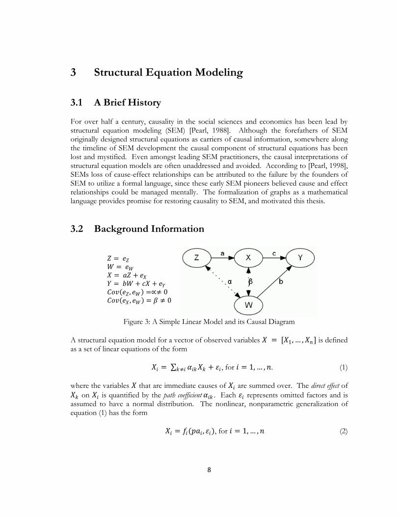
Figure 3: A Simple Linear Model and its Causal Diagram

A structural equation model for a vector of observed variables 𝑋 = [𝑋1, … , 𝑋𝑛] is defined as a set of linear equations of the form

𝑋𝑖 = 𝛼𝑖𝑘𝑋𝑘 + 𝜀𝑖𝑘≠𝑖 , for 𝑖 = 1, … , 𝑛. (1)

where the variables 𝑋 that are immediate causes of 𝑋𝑖 are summed over. The direct effect of

𝑋𝑘 on 𝑋𝑖 is quantified by the path coefficient 𝛼𝑖𝑘 . Each 𝜀𝑖 represents omitted factors and is assumed to have a normal distribution. The nonlinear, nonparametric generalization of equation (1) has the form

𝑋𝑖 = 𝑓𝑖(𝑝𝑎𝑖 , 𝜀𝑖), for 𝑖 = 1, … , 𝑛 (2)

𝑍 = 𝑒𝑍 𝑊 = 𝑒𝑊 𝑋 = 𝑎𝑍 + 𝑒𝑋 𝑌 = 𝑏𝑊 + 𝑐𝑋 + 𝑒𝑌 𝐶𝑜𝑣 𝑒𝑍 , 𝑒𝑊 =∝≠ 0 𝐶𝑜𝑣 𝑒𝑋 , 𝑒𝑊 = 𝛽 ≠ 0

9

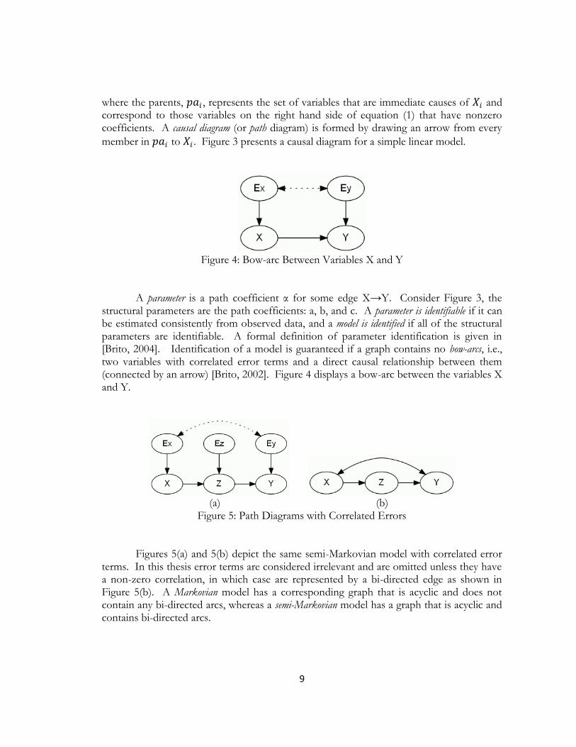
where the parents, 𝑝𝑎𝑖 , represents the set of variables that are immediate causes of 𝑋𝑖 and correspond to those variables on the right hand side of equation (1) that have nonzero coefficients. A causal diagram (or path diagram) is formed by drawing an arrow from every

member in 𝑝𝑎𝑖 to 𝑋𝑖 . Figure 3 presents a causal diagram for a simple linear model.

Figure 4: Bow-arc Between Variables X and Y

A parameter is a path coefficient α for some edge X→Y. Consider Figure 3, the structural parameters are the path coefficients: a, b, and c. A parameter is identifiable if it can be estimated consistently from observed data, and a model is identified if all of the structural parameters are identifiable. A formal definition of parameter identification is given in [Brito, 2004]. Identification of a model is guaranteed if a graph contains no bow-arcs, i.e., two variables with correlated error terms and a direct causal relationship between them (connected by an arrow) [Brito, 2002]. Figure 4 displays a bow-arc between the variables X and Y.

(a) (b)

Figure 5: Path Diagrams with Correlated Errors

Figures 5(a) and 5(b) depict the same semi-Markovian model with correlated error terms. In this thesis error terms are considered irrelevant and are omitted unless they have a non-zero correlation, in which case are represented by a bi-directed edge as shown in Figure 5(b). A Markovian model has a corresponding graph that is acyclic and does not contain any bi-directed arcs, whereas a semi-Markovian model has a graph that is acyclic and contains bi-directed arcs.

10

3.3 Problem Definition Although recent advancements in causal graph theory are foreign and unutilized by most SEM practitioners, many problems in SEM can benefit from these advancements. Following are a few issues in SEM that motivate this thesis and are discussed further in later sections.

3.3.1 Model Testing Weaknesses Finding a structural model that fits statistical data is a task often performed by SEM practitioners in two steps. The first involves finding stable path coefficient estimates through iteratively maximizing a fitness measure such as the likelihood function, and the second involves applying a statistical test to decide whether the covariance matrix implied by the parameter estimates could generate the sample covariances [Bollen, 1989; Chou and Bentler, 1995]. There are two main weaknesses to testing with this approach: (i) if a parameter is not identifiable, then stable path coefficient estimates may never be attained, potentially invalidating the entire model, and (ii) testers receive little insight as to which assumptions are violated in a misfit model [Pearl, 1998].

3.3.2 The Identification Problem Finding a necessary and sufficient criterion to determine if a causal effect can be determined from observed data has challenged researchers for over fifty years [Tian, 2005], and is known by econometricians and SEM practitioners as “The Identification Problem” [Fisher, 1966; Tian, 2005]. Although, a necessary and sufficient condition has yet to be found, [Pearl, 1998] presents a criterion able to identify a majority of structural parameters except for a few uncommon counterexamples. This thesis utilizes and implements the graphical conditions for identifying direct and total effects presented by [Pearl, 1998] and instrumental variable techniques presented in [Brito and Pearl, 2002a].

3.3.3 Nesting and Model Equivalence In SEM, a model M1 is nested in a model M2 if and only if all covariance matrices that can be generated from M1 can also be generated from M2 [Bentler, 2010]. Further, two models are equivalent if they nest each other. Currently, SEM researchers have difficulty determining if two models are covariance matrix nested or equivalent and use data in the determination [Bentler and Satorra, 2010]. The implementation presented in this thesis presents a data-free determination of model nesting and equivalence [Pearl, 1998].

11

4 Implementation The leading SEM program, known as EQS, is managed and owned by a team at UCLA consisting of Peter Bentler and Eric Wu [Bentler, 2006], and provides a user-friendly environment for simplifying, generating, estimating, and testing structural equation models. This section presents the algorithms and methods used to engineer Commentator, developed specifically for EQS.

4.1 System Overview and Input/Output The input of Commentator is a text file representing a directed acyclic graph (DAG), and the outputs are lists of all testable implications, identifiable path coefficients, identifiable total effects, and instrumental variables. The input file has the following general form:

{number of variables} {list of variable names, if any} {number of edges} {list of edges, if any} {number of measured (observable) variables} {list of measured variables, if any} {number of latent (unobservable) variables} {list of latent variables, if any} {number of required variables} {list of required variables, if any}

Figure 6 shows a sample input text file for the diagram in Figure 7, over the observable variables, V, W1, W2, X, Y, Z1 and Z2. Note that the texts in parentheses in Figure 6 are comments and are not part of the actual input. The first value read in as input is the number of variables and is used to read in the list of variable names, which for ease of programming are encoded or mapped to a specific integer value. For example in Figure 6, the variable name “V” corresponds to 0, “W1” corresponds to 1, “W2” corresponds to 2, and so on. The next value read as input corresponds to number of edges used to iterate over and read in the list of edges. If X and Y are two integer values for two different variables, then edges are represented in the input as either: (i) “X 1 Y”, or (ii) “X 2 Y”. The 1 in condition (i) implies a directed edge (right-to-left) of the form X←Y, and the 2 in condition (ii) implies a bi-directed edge of the form X↔Y. The next value read in corresponds to the number of observable variables used to iterate over and read in the observable variables. Input for latent and required variables follow this same format and usage. A variable that is required is forced to be part of all d-separating sets.

12

Figure 6: Sample Commentator Input File.

Figure 7: A Sample Path Diagram [Pearl, 2009]. (Identical to Figure 1)

7 V W1 W2 X Y Z1 Z2 (list of variables) 10 (number of edges) 5 1 0 (edge Z1←V) 6 1 0 (edge Z2←V) 5 1 1 (edge Z1←W1) 2 2 1 (edge W1↔W2) 3 2 1 (edge W1↔X) 6 1 2 (edge Z2←W2) 4 2 2 (edge W2↔Y) 4 1 3 (edge Y←X) 3 1 5 (edge X←Z1) 4 1 6 (edge Y←Z2) 7 (number of observable variables) 0 (V) 1 (W1) 2 (W2) 3 (X) 4 (Y) 5 (Z1) 6 (Z2) 0 (number of latent variables) 0 (number of required variables)

13

4.2 Graphical Notation

In probabilistic systems such as Bayesian networks, graphically discovering a set of variables that render two other disjoint sets of variables independent is a common task. The fundamental rules for graphically deducing such “separating” sets for directed acyclic graphs are encompassed in the notion of d-separation (d denoting directional) [Pearl, 1988]. Given a DAG G, let X and Y be two distinct variables in G. Further, let Z be a set of variables in G, excluding X and Y. Let a path between X and Y be defined as any sequence of consecutive edges, regardless of directionality, that connects X and Y such that no variable is revisited. A path between two variables X and Y is d-separated by a set of nodes Z when: (i) the path contains either a sequential chain i → k → j or a divergent chain or fork i ← k → j such that k is a member of Z or (ii) the path contains a collider i → k ← j such that k nor any descendants of k are members of Z. X is d-separated from Y by Z if and only if every path between X and Y is d-separated by Z [Pearl, 1988].

The computational complexity of testing d-separation between two nodes is exponential when considering all paths between two nodes in a DAG, however Definition 1 presents an algorithm for computing d-separation in time and space that is linear in the size (number of variables) of the DAG [Darwiche, 2009]. Definition 1 (Linear d-separation test) Given three disjoint sets of variables X, Y, and Z in a DAG G, testing whether X and Y are d-separated given Z can be performed using the following steps:

1. Delete any leaf nodes from G that does not belong to any of X, Y or Z. Repeat this step until no further pruning is possible.

2. Delete all outgoing edges of separating set Z.

3. Test whether X and Y are disconnected in the resulting DAG.

If X and Y are disconnected in Step 3, then Z d-separates X and Y, otherwise Z does not d-separate X and Y [Darwiche, 2009].

4.3 Removing Latent Variables

An important feature of EQS, not found in all SEM software applications, is its ability to account for latent variables, which are unobservable causes of measured variables. This subsection presents theories and algorithms for simplifying graphical structure, which bypass these latent variables and operates only on the observable or measurable variables.

14

4.3.1 Induced Path Graphs Given a directed acyclic graph G, [Verma and Pearl, 1991] have established a set of conditions involving the notion of an induced path that guarantee that two variables are not d-separated by any observable set. An induced path relative to a set of observable variables O exists between two variables A and B, if and only if there exists an undirected path U between A and B, such that each node on U belonging to O, excluding the endpoints A and B, is both a collider and an ancestor of either endpoint A or B in G [Spirtes et al., 2001]. If an induced path exists between A and B, then they must be d-connected (not d-separated) and an edge can be added between them. Adding the edge A→B implies that “every” inducing path between A and B is out of A and into B, and similarly, adding the edge A↔B implies that there “exists” an inducing path A and B that is both into A and into B. Note that a bidirectional edge is added only if latent variables are present [Spirtes et al., 2001]. An induced path graph G’ is generated from G by adding an edge between variables A and B with an arrowhead oriented at A if and only if there is an inducing path between A and B in G that is into A [Spirtes et al., 2001]. Induced path graphs preserve d-separation, such that two variables are d-separated in the induced path graph of a DAG G if and only if they are d-separated in G.

Figure 8: Path Diagram with Latent Variables C and E

Figure 9: Induced Path Graph for Figure 8 over variables A, B, F, and D

15

Figures 8 and 9 are borrowed from [Spirtes et al., 2001]. Figure 8 depicts a path diagram over the variables A, B, C, D, E and F, and Figure 9 shows the resulting induced path graph if C and E are latent variables. Note that Figure 9 results in a graph containing only observable variables. In Figure 8, an example of an induced path is the path through the variables A, B, C, D, and E respectively, since the observable variables B and D are both a collider on the path and also descendants of either A or F. This is represented by a directed edge in Figure 9 from A to F. The edge D↔F is added in Figure 9, since in Figure 8, there is an induced path through the variables D, E, and F that is both into D and into F. Figure 10 presents pseudocode for generating an induced path graph from a DAG within exponential time and space.

Figure 10: Pseudocode for Induced Path Graph

4.3.2 Maximal Ancestral Graphs (MAG) An ancestral graph G’, for a DAG G, represents and preserves the conditional independence relationships between the observable variables of G. By definition, a maximal ancestral graph (MAG) M is an ancestral graph for a DAG G if every pair of non-adjacent variables in M are d-separated by some set of variables, and it is not possible to add an edge to M without destroying the independence relationships of G [Ali et al., 2009; Tian, 2005]. MAGs preserve d-separation, such that two variables are d-separated in the MAG of a DAG G if and only if they are d-separated in G [Spirtes et al., 2001]. Three necessary and sufficient conditions for a graph M to be a MAG are given in Definition 2 [Spirtes et al., 1997; Tian, 2005].

Function: Induced-Path-Graph(G, O).

Input: A DAG G and a set of observable variables O in G.

Output: The induced path graph of G.

1. for all pairs of variables A and B in O do

2. for all undirected paths P between A and B do

3. if all member of O on P are both a collider and an ancestor of either A or B in G then

4. Add an edge to G’ according to the definition of induced path graph

5. end if

6. end for

7. end for

8. return G’

16

Definition 2 (Maximal Ancestral Graph) Given a DAG G, an ancestral graph is a MAG M for G if and only if the following

(i) There is an inducing path between two nodes A and B in M, only if they are adjacent in M.

(ii) There is a unidirectional edge in M between A and B, oriented towards B, only if A is an ancestor of B and B is not an ancestor of A in M.

(iii) There is a bidirectional edge in M between A and B, only if A is not an ancestor of B and B is not an ancestor of A in M.

[Spirtes et al., 1997a] presents a method for constructing a MAG M from a DAG G

over a set of observable variables O by: (i) adding the edge A→B in M if and only if there is an inducing path between A and B over O in G and A is an ancestor of B in G, and (ii) adding the edge in M if and only if there is an inducing path between A and B over O in G and A is an ancestor of B in G. Figure 11 provides pseudocode for generating a MAG.

Figure 11: Pseudocode for Generating a MAG

4.4 Brute Force Search Two variables in a model may be d-separated by many different sets, and when testing local models for fitness it is advantageous to use smaller separating sets to improve statistical efficiency. In this thesis, the smallest separating set between two variables is defined as the separating set that contains the fewest members compared to all other possible separating

Function: MAG (G).


Output: The MAG of G.

1. G’ Induced-Path-Graph(G, O)

2. for all adjacent nodes A and B in G’ do

3. if there exists a directed path from A to B in G then

4. Add an edge to M directed from A to B

5. else if there exists a directed path from B to A in G then

6. Add an edge to M directed from B to A

7. else

8. Add a bidirected edge to M between A and B

9. end if

10. end for

11. return M

17

sets between the two variables. In the current literature there are algorithms that find minimal separating sets, however no explicit algorithm exists which finds the smallest separating set between two variables. Commentator finds the smallest separating set by a breadth-first search (BFS), testing first the empty set, then all sets of size one, all sets of size two, and so on, until either a separating set is found or no possible sets are left.

Figure 12 presents the pseudocode for finding the smallest separating set using BFS with a first-in-first-out (FIFO) queue, and the d-separation test on Line 4 is calculated using Definition 1. The computational time and space complexity using BFS is exponential in the number of nodes in the input graph. However, [Tian et al., 1998] presents in Definition 3 a useful property to reduce the search space [Korf, 2008], which, in the average case, will reduce searching approximately 50 percent of the graph. Definition 3 (Ancestral Subgraph) Given two nodes A and B in a directed-acyclic graph G a set of nodes Z d-separates A and B in G if and only if Z d-separates A and B in the ancestral subgraph composed of the nodes A, B, and the ancestors of A or B [Tian et al., 1998].

Figure 12: Pseudocode for Breadth-First Search

In many cases, variables that are nonadjacent in a DAG do not have separating sets and searching for one between them becomes computationally prohibitive. Commentator prevents this by only searching for separating sets amongst the nonadjacent variables in a MAG, which are guaranteed to exist.

Function: BFS(G, A, B).

Input: A graph G.

Output: The separating sets between variables A and B in G.

1. Enqueue the empty set

2. while queue is not empty do

3. S Dequeue next element

4. if S d-separates A and B then

5. return S

6. else

7. for each observable node O in G not in S, A, or B do

8. S S ⋃ O

9. Enqueue S

10. end for

11. end if

12. end while

13. return fault

18

Figure 13: A Sample Path Diagram [Pearl, 2009]. (Identical to Figure 1)

5 Task 1: Find All Minimal Testable Implications

Input: A DAG G and a list of observable and latent variables.

Output: A list of the minimal testable implications of the model, specifically, a list of regression coefficients that must vanish, followed by a list of constraints induced by instrumental variables. Example: Consider Figure 1 as input, Commentator produces the following list:

𝑟𝑉𝑊1= 0

𝑟𝑉𝑊2= 0



𝑟𝑊1𝑍2∙𝑊2= 0

𝑟𝑊2𝑍1∙𝑊1= 0





= 𝑟𝑍1𝑊2


= 𝑟𝑍2𝑊1

𝑟𝑊2𝑍2∙ 𝑟𝑊1𝑋 = 𝑟𝑍2𝑋

𝑟𝑍1𝑋∙𝑊1∙ 𝑟𝑍1𝑉 = 𝑟𝑋𝑉

𝑟𝑍2𝑌∙𝑉𝑊2∙ 𝑟𝑍2𝑉∙𝑋 = 𝑟𝑌𝑉∙𝑋

19

5.1 Methodology For Markovian models, those without correlated error terms or bi-directed edges, [Pearl, 1998] has established a graphical criterion identifying the partial correlations that must vanish in a model, and [Spirtes et al., 1997b] extended this criterion shown in Definition 4 to include non-Markovian models. Definition 4 (Vanishing Regression Coefficients) For any linear model for a causal diagram D that may include cycles and bi-directed arcs, which are interpreted as emanating from a latent common

parent, the partial correlation 𝜌𝑋𝑌∙𝑍 must vanish if and only if node X is d-separated from node Y by the variables of Z in D [Spirtes et al., 1997b].

Figure 14 provides pseudocode for finding a list of vanishing regression coefficients given a DAG. The first two steps of Figure 14 generate a MAG from the input graph by first generating an induced path graph then converting the result into a MAG. All pairs of variables that are nonadjacent in the MAG must have a separating set and is searched for by the BFS algorithm in Section 3.4. Step 4 generates the ancestor subgraph discussed in Definition 3 to expedite and facilitate the BFS.

Figure 14: Pseudocode for Finding Vanishing Regression Coefficients

The list of constraints induced by instrumental variables follows immediately from the output provided by Task 2 and Task 4. For example consider the path coefficient on

W1→Z1 in Figure 1, Task 2 finds that “The coefficient ∝ on W1→Z1 is identifiable

controlling for the Empty Set, that is ∝= rW 1Z1”, likewise, Task 4 finds that “The

coefficient ∝ on W1→Z1 is identifiable via instrumental variable W2 controlling for the

Function: Vanishing-Regression-Coefficients(G).


Output: A list of all pairs of observable variables in G and there smallest separating set, if one exists.

1. G MAG(G, O)

2. for all non-adjacent observable pairs of variables A and B in G do

3. G’ ancestor subgraph of A and B in G

4. S BFS(G’, A, B)

5. end for

6. return S

20

Empty Set, that is ∝= rZ1W2/rW 1W 2

". Equating the two values for ∝ from Task 2 and 4

provides the constraint rW 1Z1=

rZ1W 2

rW 1W 2

, so that rW 1Z1∙ rW 1W 2

= rZ1W 2. Constraints of

this type can be found whenever Task 2 and Task 4 identify the same path coefficient.

5.2 Recommendations As mentioned earlier, model fitness testing in SEM occurs in two stages. The first stage involves finding stable parameter estimates through iteratively maximizing a fitness measure, and the second stage involves statistically comparing the covariance matrix derived from the parameter estimates to the data or sample covariances. There are two main weaknesses to the current approach in SEM fitness testing: (i) if a parameter is not identifiable the entire model is invalidated, and (ii) because the model is tested globally, errors are difficult to isolate and pinpoint. [Shipley, 1997] has suggested an alternate testing method utilizing vanishing regression coefficients, instead of testing the entire model for fitness to data, simply test for the regression coefficients that must be zero according to Definition 4.

A list of vanishing coefficients benefits model debugging, by isolating and locating where errors in a misfit model exist. Currently, if a proposed model does not fit the data accurately enough, a test, known as the Lagrange Multiplier (LM) test, iteratively tests all possible combinations of edge replacements and removals to find a best fit model, making the LM test computationally prohibitive for large models. However, the method in [Shipley, 1997] isolates errors to specific regression coefficients and potentially serves as a guide for the searching procedures of the LM test.

21

6 Task 2: Find Identifiable Path Coefficients Input: A DAG G and a list of observable and latent variables.

Output: List of path coefficients that are identifiable using simple regression. Example: Consider Figure 13 as input, Commentator produces the following list:





The coefficient ∝ on Z1→X is identifiable controlling for W1, that is ∝= 𝑟𝑍1𝑋∙𝑊1

The coefficient ∝ on Z2→Y is identifiable controlling for V W2, that is ∝= 𝑟𝑍2𝑌∙𝑉𝑊2

6.1 Methodology [Pearl, 1998] has established a graphical criterion for the identification of direct effects (or path coefficients) known as the single-door criterion. Definition 5 (Single-Door Criterion for Direct Effects) Given a path diagram G, let α be

the path coefficient of the edge X→Y, and let 𝐺∝ be the diagram that results from removing the edge X→Y. If there exists a set of variables Z such that

(i) No member of Z is a descendant of Y and

(ii) X is d-separated from Y by Z in 𝐺∝.

If Z satisfies these conditions, then α is identifiable and is equal to the regression coefficient 𝑟𝑋𝑌∙𝑍 [Pearl, 1998].

Figure 15 presents pseudocode for identifying path coefficients using the single-

door criterion; it takes a DAG as input and provides a list of all identifiable path coefficients. For every directed edge X→Y in G, it is removed from the graph, then a test for adjacency between X and Y is conducted in the MAG generated from G. If X and Y are non-adjacent in the MAG, then a separating set exists between X and Y guaranteeing that BFS will find a d-separator. The ancestor subgraph as in Definition 3 expedites the search.

22

Figure 15: Pseudocode for Single-Door Criterion

6.2 Recommendations In the current SEM literature, identification of path coefficients requires consideration of both data and model structure allowing for problems such as data degeneracy and statistical errors. Commentator’s list of identifiable path coefficients is data-free, providing benefits in diagnosis and convergence as discussed in the introduction. Commentator lists only those parameters that can be identified through the single-door criterion. Additional parameters can be identified using instrumental variables and total effects. [Pearl, 1998] suggests a systematic procedure for recognizing identifiable path coefficients as follows:

1. Using the single-door and back-door criterion, search for identifiable direct, total, and partial effects.

2. For each identified effect, place the path coefficients involved in a bucket. 3. Label the coefficients in the buckets as follows:

a. If a bucket is a singleton, label its coefficient I (denoting identifiable) b. If a bucket is not a singleton but contains only a single unlabeled

element, label that element I. c. If there are k non-redundant buckets that contain at most k unlabelled

coefficients, label these coefficients. 4. Repeat until no new labeling is possible. 5. List all labeled coefficients; these are identifiable.

This bucket elimination procedure and the identification of additional path coefficients can be implemented in future work.

Function: Single-Door-Criterion(G).


Output: A list of direct effects

1. List L

2. for all adjacent pairs of variables A→B in G do

3. G’ G with edge A→B removed

4. G’ MAG(G’, O)

5. G’ ancestor subgraph of A and B in G’

6. L BFS(G’, A, B)

7. end for

8. return L

23

7 Task 3: Find Identifiable Total Effects Input: A DAG G and a list of observable and latent variables.

Output: List of total effects that are identifiable using simple regression. Example: Consider Figure 13 as input, Commentator produces the following list:

The total effect τ of V on X is identifiable controlling for the Empty Set, that is 𝜏 = 𝑟𝑉𝑋

The total effect τ of V on Y is identifiable controlling for the Empty Set, that is 𝜏 = 𝑟𝑉𝑌





The total effect τ of Z1 on X is identifiable controlling for W1, that is 𝜏 = 𝑟𝑍1𝑋∙𝑊1



7.1 Methodology Commentator uses a graphical criterion, presented in Definition 6, for the identification of total effects known as the back-door criterion [Pearl, 1998]. The pseudocode for this task is identical to that in Figure 15, but instead of removing one edge from the graph, all edges emanating from X are removed.

Definition 6 (Back-Door Criterion for Total Effects) Given a path diagram G, let 𝐺𝑋 be the subgraph generated from G by removing all edges out of X. For any two variables X and Y in a path diagram G, the total effect of X on Y is identifiable, if there exists a set Z such that

(i) No member of Z is a descendant of X and

(ii) Z d-separates X from Y in 𝐺𝑋 .

If both conditions are satisfied, then the total effect of X on Y is identifiable [Pearl, 1998].

24

7.2 Recommendations Some total effects can be determined graphically without having to identify their individual path coefficients [Pearl, 2000]. This output is useful for detecting those cases where the individual path coefficients cannot be identified, but the total effect can. For example, in Figure 1, through traditional methods the total effect of Z1 on Y would not be identified since the path coefficient from X → Y is not. However, the output list for total effects shows that the total effect of Z1 on Y is identifiable, even though one of its components is not. Commentator lists only those total effects that can be identified through the back-door criterion. For future work, additional total effects can be identified using instrumental variables and combinations of already known total effects. These methods are shown in Chapter 5 of [Pearl, 1998].

25

8 Task 4: Find All Instrumental Variables Input: A DAG G and a list of observable and latent variables.

Output: List of all instrumental variables and the parameter they help identify. Example: Consider Figure 1 as input, Commentator produces the following list:





The coefficient ∝ on W2→Z2 is identifiable via instrumental variable X controlling for the

Empty Set, that is ∝= 𝑟𝑍2𝑋/𝑟𝑊2𝑋

The coefficient ∝ on X→Y is identifiable via instrumental variable Z1 controlling for V W1,

that is ∝= 𝑟𝑌𝑍1∙𝑉𝑊1/𝑟𝑋𝑍1∙𝑉𝑊1

The coefficient ∝ on Z1→X is identifiable via instrumental variable V controlling for the Empty

Set, that is ∝= 𝑟𝑋𝑉/𝑟𝑍1𝑉

The coefficient ∝ on Z2→Y is identifiable via instrumental variable V controlling for X, that is

∝= 𝑟𝑌𝑉∙𝑋/𝑟𝑍2𝑉∙𝑋

8.1 Methodology [Pearl, 2000a] defines a variable Z as instrumental relative to a cause X and an effect Y if: (i) Z is independent of all error terms that have an influence on Y that is not mediated by X, and (ii) Z is dependent of X. Definition 7 describes a graphical criterion for instrumental variables [Pearl, 2000b]. Figure 16 presents the pseudocode that Commentator uses to find instrumental variables; it takes a DAG as input and returns a list of all instrumental variables together with the parameters they help identify. Definition 7 (Instrumental Variable) Given a path diagram G, let α be the path coefficient of the

edge X→Y, and let 𝐺∝ be the diagram that results from removing the edge X→Y. Z is said to be an instrument relative to X→Y, conditioned on S, if:

(i) No member of S is a descendant of Y and

(ii) There exists a set S of variables that d-separates Z from Y in 𝐺∝, and S does not d-separate Z from X in G.

26

If Z satisfies these conditions, then Z is an instrument relative to the direct effect of X on Y and α is

identifiable, and is given by the ratio of regression coefficients 𝑟𝑌𝑍∙𝑆/𝑟𝑋𝑍∙𝑆 [Pearl, 1998].

Figure 16: Pseudocode for Instrumental Variables

8.2 Recommendations Instrumental variables identify some of the path coefficients that Task 2 does not. Consider Figure 1, the list of identifiable path coefficients in Task 2 shows that the path coefficient on X→Y is not identifiable, however the output of Commentator in this section’s example shows that X→Y can be identified by instrumental variable Z1 controlling for V and W1. Instrumental variables can be used for those instances where the single-door criterion fails to identify path coefficients.

Function: Instrumental-Variable(G).


Output: A list of instrumental variables

1. List L

2. for all adjacent pairs of variables A → B in G do

3. G’ G with edge A→B removed

4. G’ MAG(G’, O)

5. for all observable variables C not A or B do

6. if C is not adjacent to B in G’ and C is adjacent to A in the MAG(G) then

7. G’ ancestor subgraph of A and B in G’

8. L BFS(G’, B, C)

9. end if

10. end for

11. end for

12. return L

27

(a) (b)

Figure 17: Nested DAGs from [Pearl, 2009] (Identical to Figure 1 and 2, respectively)

9 Task 5: Test for Model Equivalence and Nestedness Input: Two DAG’s, G and G’, and a list of observable and latent variables.

Output: Determine whether G is equivalent to G’, G is nested in G’, or vice versa. (This is a derivative of Task 1, whereby a comparison is made between the testable implications embedded in G and G’) Example: Consider Figure 17(a) and 17(b) as input, Commentator produces the output shown in Table 2, and infer that the model in Figure 17(b) is nested in the model in Figure 17(a).

9.1 Methodology Current methods for testing whether a model is covariance-matrix nested or equivalent to another model is considered a difficult, if not impossible task for SEM researchers [Bentler and Satorra, 2010]. By definition, two models are covariance equivalent if every covariance matrix generated by one model can also be generated by another. According to [Pearl, 1998], two Markovian (models without correlated errors) linear-normal models are covariance equivalent if and only if they have the same sets of vanishing regression coefficients. Therefore the difficulties that SEM practitioners face regarding the determination of model equivalence is simplified to testing whether two models have the

28

same sets of vanishing regression coefficients. In semi-Markovian (models with correlated errors) models, this is only a necessary condition.

Testing for model nesting is similar to testing for model equivalence. A Markovian model X is covariance nested in a Markovian model Y if and only if every covariance matrix that is compatible with X is compatible with Y. Therefore, model X is nested in model Y only if the vanishing regression coefficients of model X are a superset of the vanishing regression coefficients of model Y. For example, although Figure 17(a) and (b) have completely different graphical structure, yet Figure 17(b) is nested in Figure 17(a) as seen in Table 2, since the vanishing regression coefficients for Figure 17(a) is a proper superset of those for Figure 17(b).

Table 2: Commentator Output: Testable Implications for Figure 17(a) and (b)

(Identical to Table 1)

9.1 Recommendations When models are equivalent they cannot be distinguished by statistical means, and choosing between them relies solely on available scientific theories. It is therefore beneficial to have the facility to determine if two proposed models are equivalent or nested, so that the best model may be chosen from a group of competing or indistinguishable models. Another standard SEM application is determining if a baseline model used in an incremental fit index is appropriately nested [Bentler and Satorra, 2010].

In causal models, conditional independencies are not the only type of constraint. Additional constraints known as dormant independencies (or Verma constraints) result from an

Commentator Output for Figure 17(b)

𝑟𝑉𝑊1= 0

𝑟𝑉𝑊2= 0



𝑟𝑉𝑌∙𝑊1𝑊2𝑋𝑍2= 0

𝑟𝑊1𝑍2∙𝑊2= 0

𝑟𝑊2𝑍1∙𝑊1= 0




𝑟𝑌𝑍1∙𝑉𝑊1𝑊2𝑋 = 0

𝑟𝑌𝑍1∙𝑊1𝑊2𝑋𝑍2= 0

Commentator Output for Figure 17(a)

𝑟𝑉𝑊1= 0

𝑟𝑉𝑊2= 0



𝑟𝑊1𝑍2∙𝑊2= 0

𝑟𝑊2𝑍1∙𝑊1= 0

𝑟𝑋𝑍2 ∙𝑉𝑊2= 0



29

intervention, written do(x), which is an operation that forces a variables X to have the value x regardless of their usual behavior in a causal model [Shpitser and Pearl, 2008]. A method for finding dormant independencies is presented in [Shpitser and Pearl, 2008], and implementation is set aside for future work.

30

10 Task 6: Find all Minimum-Size Admissible Sets of Covariates for Determining the Causal Effect of X on Y Input: A DAG G, a list of observable and latent variables, and a pair of variables, X and Y. Output: List of all minimum-size admissible sets S, such that conditioning on S removes confounding bias between X and Y. (This is a derivative of Task 2 and 3, tailored to a specific causal effect). Example 1: Consider Figure 17(b) as input, Commentator produces the following output:

The causal effect 𝑃(𝑌|𝑑𝑜(𝑋)) can be estimated by adjustment on: o V, W1, W2 o W1, W2, Z1 o W1, W2, Z2

Example 2: Consider Figure 17(a) as input, Commentator produces the following output:

The causal effect 𝑃(𝑌|𝑑𝑜(𝑋)) cannot be identified by adjustment, i.e., no admissible set exists.

10.1 Methodology This is a derivative of Task 2 and Task 3 focused on a specific causal effect. Each

admissible set S ensures a bias-free estimate of P(Y|do(X)) by controlling for S.

Figure 18: Diagram: Effect of Warm-up Exercise on Injury. [Shrier and Platt, 2008]

31

10.2 Recommendations This task is applicable not only to linear-models, but to non-parametric models as well, benefiting researchers such as epidemiologists, who face the problem of deciding which measurements to take. Since measurements vary in cost, reliability, and estimation power, some measurements are better than others, and therefore it is extremely useful to display the options available to investigators prior to taking any data. Consider a real-world example, Figure 18 from [Shrier and Platt, 2008], showing the effect of warm-up exercise on injury, Commentator returns the following output:

The causal effect 𝑃(𝐼𝑛𝑗𝑢𝑟𝑦|𝑑𝑜(𝑊𝑎𝑟𝑚 − 𝑢𝑝)) can be estimated by adjustment on: o Coach, Pregame proprioception o Coach, Fitness level o Genetics, Fitness level o Team motivation, Pregame proprioception o Team motivation, Fitness level o Neuromuscular fatigue, Connective tissue disorder o Neuromuscular fatigue, Tissue weakness

Presented are the minimum-size potential choices or options that epidemiologists can use to remove confounding bias; however these may not always be the cheapest to measure; in practice, it may be cheaper or more reliable to measure larger sets of size three or greater. With minor modification of Commentator, larger minimal sets can be identified and displayed so that epidemiologists will be able to assess the cost-effectiveness of the options available to them in any given study. Another useful extension of Commentator would consider measurements that are sufficient for identifying causal effects by methods other than adjustment. For example, measurement of Intra-game Proprioception and Neuromuscular Fatigue can be shown to be sufficient for identifying the effect of Warm-up on Injury using the Front-Door criterion described in [Pearl, 2009]. Moreover, equality among the various causal-effect estimations, each using a different measurement set or a different method of identification, can be used as a test for the correctness of the model under investigation.

32

11 Conclusion

This thesis presents one of the first attempts to apply graphical theories to SEM through software implementation. Although SEM has been the frontrunner in the social sciences for the past fifty years, this thesis offers improvements for SEM practitioners based on recently developed graphical methods, primarily the d-separation criterion. Commentator’s list of identifiable parameters and instrumental variables assists SEM researchers when testing and debugging models, and allows causal claims to be established even when the model in its entirety is not identified. Commentator’s list of testable implications provides an alternative method for model testing, aids in the determination of model nesting and equivalence, and in model debugging with the LM test. Commentator also successfully provides a complete list of identifiable total effects.

For future work, Commentator’s output lists and the implications of them require user feedback about how flexible practitioners are in switching from global-testing tradition to modern style of empirical research. Some of the algorithms, such as finding separators and finding induced paths, are exponential in the number of variables, and has yet to receive testing with larger and more complicated models. These computational limits need verification and will benefit from faster or more efficient algorithms.

Future work includes tasks that could be implemented using Commentator routines, for example given a model, return a list of all equivalent models. Another task would be to list additional identifiable path coefficients and total effects. These tasks have graphical criteria and algorithms discussed in [Pearl, 2009], but have yet to be implemented.

In summary, the output lists of Commentator lay the foundation for other graphical theories to build upon and extend. Commentator is just the first step in restoring causality to SEM, serving both as a research tool for practitioners and a pedagogical tool for students.

33

12 Appendix This code was compiled using Microsoft Visual Studio 2008. //Commentator.c #include <stdio.h>

#include <string.h>

#include <math.h>

#define MAX 128 //Up to 128 variables MAXimum

struct list_el {

int separator[MAX];

struct list_el * next;

};

typedef struct list_el node;

///////////////////////////

///Forward Declarations////

///////////////////////////

int generateMAG(int graph[MAX][MAX], int observable[MAX], int

numNodes);

int generateAnDAG(int i, int j, int graph[MAX][MAX], int numNodes);

int findInducedPath(int a, int b, int start, int end, int

graph[MAX][MAX], int visitedNodes[MAX], int n, int numNodes, int

observable[MAX]);

int findSeparatorBFS(int a, int b, int graph[MAX][MAX], int numNodes,

int forbidden[MAX], int required[MAX], FILE*fp, char

*variableNames[MAX][32], int output);

int clearGraph(int graph[MAX][MAX], int numNodes);

int copyGraph(int graph[MAX][MAX], int tempGraph[MAX][MAX], int

numNodes);

int printGraph(int graph[MAX][MAX], int numNodes);

int printUpdateGraph(int graph[MAX][MAX], int tempGraph[MAX][MAX], int

numNodes);

int inducedPath(int i, int j, int graph[MAX][MAX], int

visitedNodes[MAX], int n, int numNodes, int observable[MAX], int

direction);

int ancestor(int a, int b, int graph[MAX][MAX], int numNodes);

int dSeparates(int a, int b, int s[MAX], int graph[MAX][MAX], int

numNodes);

int disconnected(int a, int b, int graph[MAX][MAX], int

visitedNodes[MAX], int numNodes);

////////////////

//main program//

////////////////

34

int main(int argc, char **argv)

{

//file pointers

FILE *outFile;

FILE *outFile2;

FILE *inFile;

//iterators

int index = 0;

int i,j,k,x,y;

int iter = 0;

int temp;

//pointers

int *numEdges;

int *numForbidden;

int *numRequired;

int *numObservable;

int numNodes;

//data structures - change values to accomodate larger path

diagrams

int edge[MAX];

int from[MAX];

int to[MAX];

int inputGraph[MAX][MAX];

int graph[MAX][MAX];

int tempGraph[MAX][MAX];

int forbidden[MAX];

int observable[MAX];

int required[MAX];

int practice[MAX]; // for debugging

char c;//for printing file storages.

char *variableNames[MAX][32];

char *name[32];

//////////////////////////////

/////FILE NAME HERE //////////

//////////////////////////////

inFile = fopen("warmup.txt","r");

//////////////////////////////

/////FILE NAME HERE //////////

//////////////////////////////

35

fscanf(inFile, "%i\n", &numNodes);

printf("Total number of nodes = %i\n\n", numNodes);

for (index = 0; index < numNodes; ++index) {

if (fmod((double)index, (double)10) == 0) {

fscanf(inFile, "%s\n", name);

} else {

fscanf(inFile, "%s ", name);

}

strcpy(variableNames[index], name);

}

fscanf(inFile, "%i\n", &numEdges);

printf("Total number of edges = %i\n\n", numEdges);

for (index = 0; index < numEdges; ++index)

fscanf(inFile, "%i %i %i\n", &(to[index]), &(edge[index]),

&(from[index]));

fscanf(inFile, "%i\n", &numObservable);

for (index = 0; index < numNodes; ++index) observable[index] =

0; //initialize observable list to all observable

for (index = 0; index < numObservable; ++index) {

fscanf(inFile, "%i\n", &temp);

observable[temp] = 1;

}

printf("\nNumObservable = %i\n",numObservable);

printf("Observable (Measureable) Nodes: ");


if (observable[index] != 0) printf("%i ", index);

}

printf("\n");

fscanf(inFile, "%i\n", &numForbidden);


forbidden[index] = 0; //clear forbidden list

}

for (index = 0; index < numForbidden; ++index) {


forbidden[temp] = 1;

}

printf("\nNumForbidden = %i\n",numForbidden);

printf("Forbidden (Unobservable/Latent) Nodes: ");


if (forbidden[index] != 0) printf("%i ", index);

}

printf("\n");

fscanf(inFile, "%i\n", &numRequired);

36

//clear forbidden list

for (index = 0; index < numNodes; ++index) required[index] = 0;

for (index = 0; index < numRequired; ++index) {


required[temp] = 1;

}

printf("\nNumRequired = %i\n",numRequired);

printf("Required Nodes: ");


if (required[index] != 0) printf("%i ", index);

}

printf("\n\n");

fclose(inFile);

//Initialize Matrix with "0" for "empty edges"

clearGraph(graph, numNodes);

printf("Input Graph:\n");

for (index = 0; index < numEdges; ++index){

if (edge[index] == 2) {

printf("%s <--> %s\n", variableNames[from[index]],

variableNames[to[index]]);

graph[from[index]][to[index]] = 2;

graph[to[index]][from[index]] = 2;

} else if (edge[index] == 1){

printf("%s ---> %s\n", variableNames[from[index]],

variableNames[to[index]]);

graph[from[index]][to[index]] = 1;

} else {

printf("invalid edge");

}

}

//copy and store original graph in inputGraph

copyGraph(graph, inputGraph, numNodes);

//print out edge graph

printf("\nMatrix (graph):\n");

printGraph(graph, numNodes);

////////////////////////////

////Testable Implications///

////////////////////////////

generateMAG(graph, observable, numNodes); //graph now is a MAG

37

outFile = fopen("testableImplications.txt", "w");

fprintf(outFile, "The following regression coefficients should

vanish:\n");

for (i = 0; i < numNodes; ++i){

for(j = i + 1; j < numNodes; ++j){ //iterate over all

pairs of nodes

if(observable[i] == 1 && observable[j] == 1 &&

graph[i][j] == 0 && graph[j][i] == 0){

//Finding vanishing coefficients

copyGraph(graph,tempGraph, numNodes);

generateAnDAG(i, j , tempGraph, numNodes);

findSeparatorBFS(i, j, tempGraph, numNodes,

forbidden, required, outFile, variableNames, 0);

}

}

}

//Finding constraints induced by Instrumental Variables

for (i = 0; i < numNodes; ++i) {

for(j = 0; j < numNodes; ++j){ //iterate over all pairs

(actually... adjacent) of nodes

if(i != j && observable[i] == 1 && observable[j] ==

1 && inputGraph[i][j] == 1){

//copies original inputGraph into graph

copyGraph(inputGraph, graph, numNodes);

//remove edge i --> j

graph[i][j] = 0;

//preprocessing

generateMAG(graph, observable, numNodes);

for (k = 0; k < numNodes; ++k){

if (observable[k] != 0 && k != i && k !=

j // k must be observable instrument

&& graph[k][j] == 0 && graph[j][k]

== 0 // test k d-separated form j

&& (tempGraph[i][k] != 0 ||

tempGraph[k][i] != 0) //test k d-connected to i

&& !(ancestor(i, k, tempGraph,

numNodes))) {

findIVSeparatorBFS(k, i, j,

graph, numNodes, forbidden, required, outFile, variableNames, 0);

}

}

}

}

}

fclose(outFile);

38

copyGraph(graph, tempGraph , numNodes); //need for instrumental

variables

///////////////////////////////

////Direct Effects ////////////

///////////////////////////////

outFile = fopen("identifiableParameters.txt", "w");

fprintf(outFile, "The following parameters are

identifiable:\n");

//printf("\nFinding Instrumental Variables:\n");

outFile2 = fopen("instrumentalVariables.txt", "w");

fprintf(outFile2, "The following are instrumental

variables:\n");


for(j = 0; j < numNodes; ++j){ //iterate over all pairs

(actually... adjacent) of nodes

if(i != j && observable[i] == 1 && observable[j] ==

1 && inputGraph[i][j] == 1){



//remove edge i --> j

graph[i][j] = 0;

//preprocessing


//Test for disconnectedness in graph

if ((graph[i][j] ==0) && (graph[j][i] == 0)){

//Uncomment this if a specific back door

separator is needed.

generateAnDAG(i,j,graph, numNodes);

findSeparatorBFS(i, j, graph, numNodes,

forbidden, required, outFile, variableNames, 1);

}

for (k = 0; k < numNodes; ++k){

if (observable[k] != 0 && k != i && k !=

j // k must be observable instrument

&& graph[k][j] == 0 && graph[j][k]

== 0 // test k d-separated form j

&& (tempGraph[i][k] != 0 ||

tempGraph[k][i] != 0) //test k d-connected to i

&& !(ancestor(i, k, tempGraph,

numNodes))) {

39

findIVSeparatorBFS(k, i, j,

graph, numNodes, forbidden, required, outFile2, variableNames, 1);

}

}

}

}

}

fclose(outFile);

fclose(outFile2);

///////////////////////////////////

///// Total Effects //////////////

/////////////////////////////////

//printf("\nFinding Total Effects:\n");

outFile = fopen("identifiableTotalEffects.txt", "w");

fprintf(outFile, "The following total effects are

identifiable:\n");

//first iterate over all/each variable i


if (observable[i] == 1) {

//copy inputGraph to graph


//remove all edges out of i

for (j = 0; j < numNodes; ++j) {

if (graph[i][j] == 1) {

graph[i][j] = 0;

}

}

//generate MAG


for(j = 0; j < numNodes; ++j){

if((observable[j] == 1) && (j != i) &&

(graph[i][j] == 0) && (graph[j][i] == 0)){

//copyGraph

copyGraph(graph,tempGraph,numNodes);

//generate Ancestor DAG

generateAnDAG(i, j,tempGraph, numNodes);

//Run test for total effects

if (ancestor(i, j, inputGraph, numNodes)

&& (graph[i][j] ==0) && (graph[j][i] == 0)) {

40

//Test to find back door

separators

findSeparatorBFS(i, j, tempGraph,

numNodes, forbidden, required, outFile, variableNames, 2);

}

}

}

}

}

fclose(outFile);

//////////////////////////////

////Minimal Admissible Sets///

//////////////////////////////

//set x --> y to to be removed

x = 10;

y = 12;



if (graph[x][y] != 0) {//remove edge x --> y

graph[x][y] = 0;

}else { // remove all outgoing edges


if (graph[x][i] == 1) {

graph[x][i] = 0;

}

}

}

//preprocessing


//Test for disconnectedness in graph

outFile = fopen("minimalAdmissibleSets.txt", "w");

fprintf(outFile, "The causal effect P(%s|do(%s)) can be

estimated by adjustment on:\n", variableNames[y], variableNames[x]);

if ((graph[x][y] ==0) && (graph[y][x] == 0)){

generateAnDAG(x,y,graph, numNodes);

findSeparatorBFS(x, y, graph, numNodes, forbidden,

required, outFile, variableNames, 4);

}

fclose(outFile);

/////////////////////////////

//// output files ///////////

41

/////////////////////////////

printf("\n");

inFile = fopen("testableImplications.txt", "r");

while((c = getc(inFile)) != EOF) {

putchar(c);

}

fclose(inFile);

printf("\n");

inFile = fopen("identifiableParameters.txt", "r");


putchar(c);

}

fclose(inFile);

printf("\n");

inFile = fopen("identifiableTotalEffects.txt", "r");


putchar(c);

}

fclose(inFile);

printf("\n");

inFile = fopen("instrumentalVariables.txt", "r");


putchar(c);

}

fclose(inFile);

printf("\n");

inFile = fopen("minimalAdmissibleSets.txt", "r");


putchar(c);

}

fclose(inFile);

return 0;

}

// generates a MAG from graph

int generateMAG(int graph[MAX][MAX], int observable[MAX], int

numNodes){

////////////////////////

///Induced Path Graph///

////////////////////////

42

FILE *inFile;

int i, j, k, h;

int index;

int isInducer;

int visitedNodes[MAX];

int n;

int *num;

int *temp;


int path[MAX];

int bidirected;

int inducingPath;

int aAncestor;

int bAncestor;

clearGraph(tempGraph,numNodes);


for(j = i + 1; j < numNodes; ++j){ //Iterate over all

pairs of nodes

if (observable[i] == 1 && observable[j] == 1) {

aAncestor = 0;

bAncestor = 0;

//add i to the list and initialize n;

visitedNodes[0] = i;

n = 1;

//find all paths between i and j and store it

in inFile

if (findInducedPath(i, j, i, j, graph,

visitedNodes, n, numNodes, observable)) {

//add edges

if (ancestor(i, j, graph, numNodes)){

aAncestor = 1;

}

if (ancestor(j, i, graph, numNodes)){

bAncestor = 1;

}

if (aAncestor == 1) {

tempGraph[i][j] = 1;

} else if (bAncestor == 1) {

tempGraph[j][i] = 1;

} else {

tempGraph[i][j] = 2;

tempGraph[j][i] = 2;

}

}

}

43

}

}

copyGraph(tempGraph, graph, numNodes); //copy values from

tempGraph to graph

return 1;

}

//finds induced path recursively between start and end.

int findInducedPath(int a, int b, int start, int end, int

graph[MAX][MAX], int visitedNodes[MAX], int n, int numNodes, int

observable[MAX]) {

int i,j;

int visited;

int colliders;

int ancestors;

//FILE *fp;

if(a != b) {


if (i == a && (graph[a][b] != 0 || graph[b][a] !=

0)){

ancestors = 1;

colliders = 1;

visitedNodes[n] = end;

for(j = 1; j < n; ++j) {

if (observable[visitedNodes[j]] == 1) {

if (graph[visitedNodes[j-

1]][visitedNodes[j]] == 0 || graph[visitedNodes[j+1]][visitedNodes[j]]

== 0) {

colliders = 0;

}

if ((ancestor(visitedNodes[j],

start, graph,numNodes) == 0) && (ancestor(visitedNodes[j], end, graph,

numNodes) == 0)){

ancestors = 0;

}

}

}

if (ancestors == 1 && colliders == 1) {

return 1;

}

}

visited = 0;

for (j = 0; j < n; j++){

if (visitedNodes[j] == i) visited = 1;

44

}

if((graph[a][i] != 0 || graph[i][a] != 0) && (i !=

a) && (visited == 0)) {

visitedNodes[n] = i;

n = n + 1;

if (findInducedPath(i, b, start, end, graph,

visitedNodes, n, numNodes, observable) == 1) return 1;

n = n -1;

visitedNodes[n] = 0;

}

}

}

return 0;

}

// generates Ancestor DAG of i and j from 'graph'

int generateAnDAG(int i, int j, int graph[MAX][MAX], int numNodes){

int iter, index;


//copy graph over to tempGraph;

copyGraph(graph, tempGraph, numNodes);

for (index = 0; index < numNodes; ++index){

if ((index != i) && (index != j)){

if (!(ancestor(index, i, graph, numNodes)) &&

!(ancestor(index,j, graph,numNodes))){

for (iter = 0; iter < numNodes; ++iter){

//Remove edges and nodes

tempGraph[iter][index] = 0;

tempGraph[index][iter] = 0;

}

}

}

}

//copy tempGraph back over to graph

copyGraph(tempGraph, graph, numNodes);

return 1;

}

//finds all minimum separators between a and b in graph via breadth-

first search

45

int findSeparatorBFS(int a, int b, int graph[MAX][MAX], int numNodes,

int forbidden[MAX], int required[MAX], FILE *fp, char

*variableNames[MAX][32], int output) {

//output = 0 --> testable implications

//output = 1 --> identiable parameters

//output = 2 --> identifiable total effects

//output = 3 --> instrumental variables (has been implmented in

findIVSeparatorBFS(...));

//output = 4 --> admissible sets

//output = 5 --> returns 1 single-door separator between a and

b.

node *current, *head, *tail;

int i,j,k;


int depth;

int currentDepth;

int maxVal;

head = NULL;

tail = NULL;

current = (node*)malloc(sizeof(node));


current->separator[i] = 0; //Initialize separator to empty

set

if (required[i] != 0)

current->separator[i] = 1;

}

current->next = NULL;

head = current;

tail = current;

depth = -1;

while (current){

if (depth > -1) {

currentDepth = 0;


if (current->separator[i] != 0) {

currentDepth = currentDepth + 1;

}

}

if(currentDepth > depth) {

fprintf(fp, "\n");

return 1;

}

}

if (dSeparates(a, b, current->separator, graph, numNodes))

{

46

if (output == 0) { //Print list of vanishing

regression coefficients

if (depth > -1) { //a separator has been found

before

fprintf(fp, "\n");

}

fprintf(fp, "%R_%s.%s", variableNames[a],

variableNames[b]);

j = 0;

for (i = 0; i < numNodes; ++i) if (current-

>separator[i] != 0) j = j + 1;

if (j != 0) fprintf(fp, "*");

k = 0;



if (k < j - 1) {

fprintf(fp, "%s.",

variableNames[i]);

} else {

fprintf(fp, "%s",

variableNames[i]);

}

k = k + 1;

}

}

depth = j;

if (j == 0) fprintf(fp, " "); //The empty set

fprintf(fp, "= 0");

} else if (output == 1){

if (depth > - 1) {

fprintf(fp,"\n");

}

fprintf(fp, "-*- The coefficient alpha on %s--

>%s is identifiable controlling for", variableNames[a],

variableNames[b]);

j = 0;



fprintf(fp, " %s",

variableNames[i]);

j = j + 1;

}

}

depth = j;

if (j == 0) fprintf(fp, " the Empty Set");

47

fprintf(fp, ", that is alpha = R_%s.%s",

variableNames[a], variableNames[b]);

if (j == 0) {

fprintf(fp, " ");

} else {

fprintf(fp, "*");

k = 0;



if (k < j - 1) {

fprintf(fp, "%s.",

variableNames[i]);

} else {

fprintf(fp, "%s",

variableNames[i]);

}

k = k + 1;

}

}

}


if (depth > - 1) {

fprintf(fp,"\n");

}

fprintf(fp, "-*- The total effect, tau, of %s

on %s is identifiable controlling for", variableNames[a],

variableNames[b]);

j = 0;



fprintf(fp, " %s",

variableNames[i]);

j = j + 1;

}

}

depth = j;


fprintf(fp, ", that is tau = R_%s.%s",

variableNames[a], variableNames[b]);

if (j == 0) {

fprintf(fp, " ");

} else {

fprintf(fp, "*");

k = 0;



if (k < j - 1) {

fprintf(fp, "%s.",

variableNames[i]);

} else {

48

fprintf(fp, "%s",

variableNames[i]);

}

k = k + 1;

}

}

}


//has been implmented in

findIVSeparatorBFS(...)

} else if (output == 4) {

if (depth > - 1) {

fprintf(fp,"\n");

}

j = 0;

fprintf(fp, " *");



fprintf(fp, "%s ",

variableNames[i]);

j = j + 1;

}

}

depth = j;

if (j == 0) fprintf(fp, "the Empty Set ");


j = 0;



j = j + 1;

}

}

depth = j;

fprintf(fp, "R_%s.%s", variableNames[a],

variableNames[b]);

if (j == 0) {

fprintf(fp, " ");

} else {

fprintf(fp, "*");

k = 0;



if (k < j - 1) {

fprintf(fp, "%s.",

variableNames[i]);

} else {

fprintf(fp, "%s",

variableNames[i]);

}

k = k + 1;

}

49

}

}

return 1;

}

} else {

//Enqueue

maxVal = 0;

//Find the maxVal


if (current->separator[i] != 0) maxVal = i;

}

for (i = maxVal; i < numNodes; ++i) {

if ((current->separator[i] == 0) && (i != a &&

i != b)) { //create new node and add it to queue

head = (node*)malloc(sizeof(node));

for (k = 0; k < numNodes; ++k) {

head->separator[k] = current-

>separator[k];

}

head->separator[i] = 1;

head->next = NULL;

tail->next = head;

tail = tail->next;

visitedNodes[i] = 1;

}

}

}

//Dequeue current node

head = current;

current = current->next;

head->next = NULL;

free(head);

}

fprintf(fp, "\n");

return 1;

}

// finds separator using instrumental variable IV, between X and Y, in

graph.

int findIVSeparatorBFS(int IV, int x, int y, int graph[MAX][MAX], int

numNodes, int forbidden[MAX], int required[MAX], FILE *fp, char

*variableNames[MAX][32], int output) {

// if output == 0, then output testable constraints via

instrumental variables

// if output == 1, then output IV

node *current, *head, *tail;

int i,j,k;


50

int depth;

int currentDepth;

int maxVal;

FILE* outFile;

head = NULL;

tail = NULL;

current = (node*)malloc(sizeof(node));


current->separator[i] = 0; //Initialize separator to empty

set

if (required[i] != 0)

current->separator[i] = 1;

}

current->next = NULL;

head = current;

tail = current;

depth = -1;

while (current){

if (depth > -1) {

currentDepth = 0;



currentDepth = currentDepth + 1;

}

}

if(currentDepth > depth) {

//fprintf(fp, "\n");

return 1;

}

}

if (dSeparates(IV, y, current->separator, graph,

numNodes)) {

if (output == 0) {

//fprintf(fp, "Hello worlds\n");

if (graph[x][y] == 0 && graph[y][x] == 0) {

//then a d-separator exists

fprintf(fp, "(");

findSeparatorBFS(x, y, graph, numNodes,

forbidden, required, fp, variableNames, 5);

fprintf(fp, ") * (R_%s.%s",

variableNames[x], variableNames[IV]);

}

51

j = 0;

for (i = 0; i < numNodes; ++i) if (current-

>separator[i] != 0) j = j + 1;


k = 0;



if (k < j - 1) {

fprintf(fp, "%s.",

variableNames[i]);

} else {

fprintf(fp, "%s",

variableNames[i]);

}

k = k + 1;

}

}

fprintf(fp, ") = (R_%s.%s", variableNames[y],

variableNames[IV]);


k = 0;



if (k < j - 1) {

fprintf(fp, "%s.",

variableNames[i]);

} else {

fprintf(fp, "%s",

variableNames[i]);

}

k = k + 1;

}

}

fprintf(fp, ")\n");

return 1;


if (depth > -1) { //a separator has been found

before

fprintf(fp, "\n");

}

fprintf(fp, "-*- The coefficient alpha on %s--

>%s is identifiable via instrumental variable %S controlling for",

variableNames[x], variableNames[y], variableNames[IV]);

52

j = 0;



fprintf(fp, " %s",

variableNames[i]);

j = j + 1;

}

}

depth = j;


//The empty set

fprintf(fp, ", that is alpha = (R_%s.%s",

variableNames[y], variableNames[IV]);


k = 0;



if (k < j - 1) {

fprintf(fp, "%s.",

variableNames[i]);

} else {

fprintf(fp, "%s",

variableNames[i]);

}

k = k + 1;

}

}

fprintf(fp, ") / (R_%s.%s", variableNames[x],

variableNames[IV]);


k = 0;



if (k < j - 1) {

fprintf(fp, "%s.",

variableNames[i]);

} else {

fprintf(fp, "%s",

variableNames[i]);

}

k = k + 1;

}

}

fprintf(fp, ")\n");

}

} else {

//Enqueue

maxVal = 0;

53

//Find the maxVal


if (current->separator[i] != 0) maxVal = i;

}

for (i = maxVal; i < numNodes; ++i) {

if ((current->separator[i] == 0) && (i != IV

&& i != y)) { //create new node and add it to queue

head = (node*)malloc(sizeof(node));

for (k = 0; k < numNodes; ++k) {

head->separator[k] = current-

>separator[k];

}

head->separator[i] = 1;

head->next = NULL;

tail->next = head;

tail = tail->next;


}

}

}

//Dequeue current node

head = current;

current = current->next;

head->next = NULL;

free(head);

}

//fprintf(fp, "\n");

return 1;

}

//clears graph to all 0

int clearGraph(int graph[MAX][MAX], int numNodes){

int col, row;

for (row = 0; row < numNodes; ++row)

for(col = 0; col < numNodes; ++col)

graph[row][col] = 0;

return 1;

}

//copy values over from graph to tempGraph

int copyGraph(int graph[MAX][MAX], int tempGraph[MAX][MAX], int

numNodes){

int col, row;

for (row = 0; row < numNodes; ++row)

for(col = 0; col < numNodes; ++col)

tempGraph[row][col] = graph[row][col];

return 1;

}

54

//print out Graph

int printGraph(int graph[MAX][MAX], int numNodes){

int col, row;

for (col = 0; col < numNodes; ++col){

for(row = 0; row < numNodes; ++row){

printf("%i ", graph[row][col]);

}

printf("\n");

}

return 1;

}

//copy values over from tempGraph to graph and print graph.

int printUpdateGraph(int graph[MAX][MAX], int tempGraph[MAX][MAX], int

numNodes) {

int col, row;


for(row = 0; row < numNodes; ++row){

graph[row][col] = tempGraph[row][col];

tempGraph[row][col] = 0;

printf("%i ", graph[row][col]);

}

printf("\n");

}

return 1;

}

//returns 1 if A is an ancestor of B

int ancestor(int a, int b, int graph[MAX][MAX], int numNodes) {

int i;

int retVal = 0;

if (graph[a][b] == 1) return 1; //BASE CASE

for (i = 0; i < numNodes; ++i){ //Iterate over all children

if (graph[a][i] == 1) { // INDUCTIVE CASE

if(ancestor(i, b, graph, numNodes)) return 1;

}

}

return 0;

}

// returns 1 if s[] d-separates a and b in graph, 0 otherwise.

int dSeparates(int a, int b, int s[MAX], int graph[MAX][MAX], int

numNodes) {

/*

ALGORITHM:

1) Delete all leaf nodes not an element of X, Y, or evidence Z

2) Delete all outgoing edges leaving evidence Z

3) Test if X and Y are disconnected

55

*/

int index, iter;

int row, col;

int ancestors;

int i;



s[a] = 1;

s[b] = 1;

copyGraph(graph, tempGraph, numNodes);

for (index = 0; index < numNodes; ++index){

if(s[index] == 0) {

ancestors = 0;


if(s[i] != 0) {

if (ancestor(index, i, graph, numNodes))

{

ancestors = ancestors + 1;

}

}

}

if (ancestors == 0) { //That means it is a leaf

node

for (iter = 0; iter < numNodes; ++iter){

//Remove edges and nodes

tempGraph[iter][index] = 0;

tempGraph[index][iter] = 0;

}

}

}

}

//DELETE ALL EDGES comming out of evidence (s[])

s[a] = 0;

s[b] = 0;


if (s[col] != 0){

for(row = 0; row < numNodes; ++row) {

if (tempGraph[col][row] == 1)

tempGraph[col][row] = 0;

}

}

}

//TEST IF A and B are disconnected

56

for(i = 0; i < numNodes; ++i) //initialize visitedNodes[]


if (disconnected(a, b, tempGraph, visitedNodes, numNodes)) {

return 1;

}

return 0;

}

//returns 1 if a and b are disconnected in graph, 0 otherwise

int disconnected(int a, int b, int graph[MAX][MAX], int

visitedNodes[MAX], int numNodes) {

int i;

int numNeighbors = 0;

visitedNodes[a] = 1;

if (graph[a][b] != 0 || graph[b][a] != 0) return 0;//BASE CASE:

check if a and b are connected

for (i = 0; i < numNodes; ++i) //count the number of neighbors

if (graph[a][i] != 0 || graph[i][a] != 0) numNeighbors =

numNeighbors + 1;

if (numNeighbors == 0) return 1; //disconnected, since no

neighbors


if ((graph[a][i] != 0 || graph[i][a] != 0) &&

visitedNodes[i] == 0) {

if (disconnected(i, b, graph, visitedNodes,

numNodes) == 0) return 0;

}

}

return 1;

}

57

13 References [Ali et al., 2009] R. Ali, T. Richardson, and P. Spirtes. “Markov Equivalence for Ancestral

Graphs”. The Annals of Statistics, Vol. 37, No. 5B, 2808-2837, 2009. [Bentler and Satorra, 2010] P. Bentler and A. Satorra. “Testing Model Nesting and

Equivalence” in Psychological Methods. UCLA Department of Statistics, Los Angeles, CA, USA, 2010.

[Bentler, 2006a] P. Bentler. EQS Structural Equations Program Manual. Multivariate

Software, Inc., Encino, CA, USA, 2006. [Bentler, 2006b] P. Bentler. EQS software version 6.1, 2006. URL http://

www.mvsoft.com/products.htm. [Bentler and Wu, 2006] P. Bentler and E. Wu. EQS software “User’s Guide”. Multivariate Software, Inc., Encino, CA, USA, 2006. [Brito, 2004] C. Brito. “Graphical Methods for Identification in Structural Equation

Models”. Ph.D. Thesis, UCLA Computer Science Department, Technical Report (R-314), Los Angeles, CA, USA, 2004.

[Brito and Pearl, 2002a] C. Brito and J. Pearl. “Generalized Instrumental Variables”.

UCLA Cognitive Systems Laboratory, Technical Report (R-303), April 2002. In A. Darwiche and N.Friedman (Eds.), Uncertainty in Artificial Intelligence, Proceedings of the Eighteenth Conference, Morgan Kaufmann: San Francisco, CA, USA, 85-93, August 2002.

[Brito and Pearl, 2002b] C. Brito and J. Pearl. “A New Identification Criterion for

Recursive Models with Correlated Error”. UCLA Cognitive Systems Laboratory, Technical Report (R-291), October 2001. Structural Equation Modeling, 9(4), 459-474, 2002.

[Bollen, 1989] K. Bollen. Structural Equations with Latent Variables. John Wiley & Sons

Publication, New York, NY, USA, 1989. [Chou and Bentler, 1995] C. Chou and P. Bentler. “Estimation and Test in Structural

Equation Modeling”. Structural Equation Modeling. Sage Publications, Thousand Oaks, CA, USA, pp. 37-55, 1995.

[Darwiche, 2009] A. Darwiche. Modeling and Reasoning with Bayesian Networks. Cambridge

University Press, New York, NY, USA 2009.

58

[Duncan, 1975] O. Duncan. Introduction to Structural Equation Models. Academic Press, New York, NY, USA, 1975.

[Fisher, 1966] F. Fisher. The Identification Problem in Econometrics. McGraw-Hill Publication,

New York, NY, USA, 1966. [Hoyle, 1995] R. Hoyle. Structural Equation Modeling. SAGE Publications, Inc., Thousand

Oaks, CA, USA, 1995. [Kenny, 1979] D. Kenny. Correlation and Causality. John Wiley & Sons Publication, New

York, NY, USA, 1979. [Korf, 2008] R. Korf. Heuristic Search. Academic Publishing, University of California, Los

Angeles, CA, USA, 2008. [Pearl, 2009] J. Pearl. Causality: Models, Reasoning, and Inference. Second Edition. Cambridge

University Press, New York, NY, USA, 2009. [Pearl, 2000a] J. Pearl. Causality: Models, Reasoning, and Inference. Cambridge University

Press, New York, NY, USA, 2000. [Pearl, 2000b] J. Pearl. “Parameter Identification: A New Perspective”. UCLA Cognitive

Systems Laboratory, Technical Report (R-276), 2000. [Pearl, 1998] J. Pearl. "Graphs, Causality, and Structural Equation Models". UCLA

Cognitive Systems Laboratory, Technical Report (R-253), June 1998. Sociological Methods and Research, Vol. 27, No. 2, pp. 226-284, November 1998.

[Pearl, 1988] J. Pearl. Probabilistic Reasoning in Intelligent Systems: Networks of Plausible Inference.

Morgan Kaufmann Publishers Inc., San Francisco, CA, USA, 1988. [Shipley, 1997] B. Shipley. “An Inferential Test for Structural Equation Models Based on

Directed Acyclic Graphs and its Nonparametric Equivalents”. Technical report, Department of Biology, University of Sherbrooke, Quebec, Canada, 1997.

[Shpitser and Pearl, 2008] I. Shpitser and J. Pearl. "Dormant Independence". UCLA

Cognitive Systems Laboratory, Technical Report (R-340), April 2008. In Proceedings of the Twenty-Third Conference on Artificial Intelligence, 1081-1087, 2008.

[Shrier and Platt, 2008] I. Shrier and R. Platt. “Reducing bias through directed acyclic

graphs”. BMC Medical Research Methods, 2008.

59

[Spirtes et al., 2001] P. Spirtes, C. Glymour, and R. Scheines. Causation, Prediction, and Search. MIT Press, Cambridge, MA, USA, 2001.

[Spirtes et al., 1997a] P. Spirtes, T. Richardson, and C. Meek. “The Dimensionality of

Mixed Ancestral Graphs”. Technical Report CMU-PHIL-83, Department of Philosophy Carnegie Mellon University, Pittsburg, PA, USA, 1997.

[Spirtes et al., 1997b] P. Spirtes, T. Richardson, C. Meek, R.Scheines, and C. Glymour.

“Using Path Diagrams as a Structural Equation Modeling Tool”. Technical Report CMU-PHIL-82, Department of Philosophy, Carnegie Mellon University, Pittsburgh, USA, 1997.

[Spirtes et al., 1996] P. Spirtes, T. Richardson, C. Meek, R. Scheines, and C. Glymour.

“Using d-separation to Calculate Zero Partial Correlations in Linear Models with Correlated Errors”. Technical Report CMU-PHIL-72, Department of Philosophy, Carnegie Mellon University, Pittsburgh, USA, 1996.

[Tian, 2007] J. Tian. “A Criterion for Parameter Identification in Structural Equation

Models”. Proceedings of the Conference on Uncertainty in Artificial Intelligence (UAI). Vancouver, Canada. AUAI Press, pp. 392- 399. July 19-22, 2007.

[Tian, 2005] J. Tian. “Generating Markov Equivalent Maximal Ancestral Graphs by Single

Edge Replacement”. Proceedings of the Conference on Uncertainty in Artificial Intelligence (UAI), July 26-29, 2005. Edinburgh, Scotland, AUAI Press, 284-291, 2005.

[Tial et al., 1998] J. Tian, A. Paz, and J. Pearl. “Finding a Minimal D-separator”. Technical

Report. R-254 University of California, Los Angeles, Computer Science Department, Los Angeles, CA, USA, 1998.

[Tian and Pearl, 1991] T. Verma & J. Pearl. “Equivalence and Synthesis of Causal

Models”. UCLA Cognitive Systems Laboratory, Technical Report (R-150), June 1990, in Proceedings, Workshop on Uncertainty in Artificial Intelligence, July 27-29, 1990. Also in Uncertainty in Artificial Intelligence, 6, Cambridge, MA, Elsevier Science Publishers, 220-227, 1991.

[Wright, 1921] S. Wright. “Correlation and Causation”. Journal of Agricultural Research,

20:557-585, 1921.

a front-end user-interface module for graphical and structural

Documents