a “function” has: a source a target a rule to go from the source to the target
Post on 20-Dec-2015
221 views
TRANSCRIPT

A “function” has:
•A source
•A target
•A rule to go from the source to the target
)(xfy 0
0.5
1
1.5
2
2.5
-0.5 0 0.5 1 1.5
3.02 xy

The source and target can be 2 or 3 dimensional
),( yxfH H can be a topographic map, for example
For each point on the map we assign a number

)(),,( tfZYX The other way around:
The orbit describes the movement of the planets as a function of time in 3-D

Lets consider functions from 2-D to 2-D:
),(
),(
),(),(
yxfY
yxfX
YXyxf
y
x
y
xIf we can write:
fyexdY
cybxaX
Then f is called linear

2 important functions from 2-D to 2-D
y
x
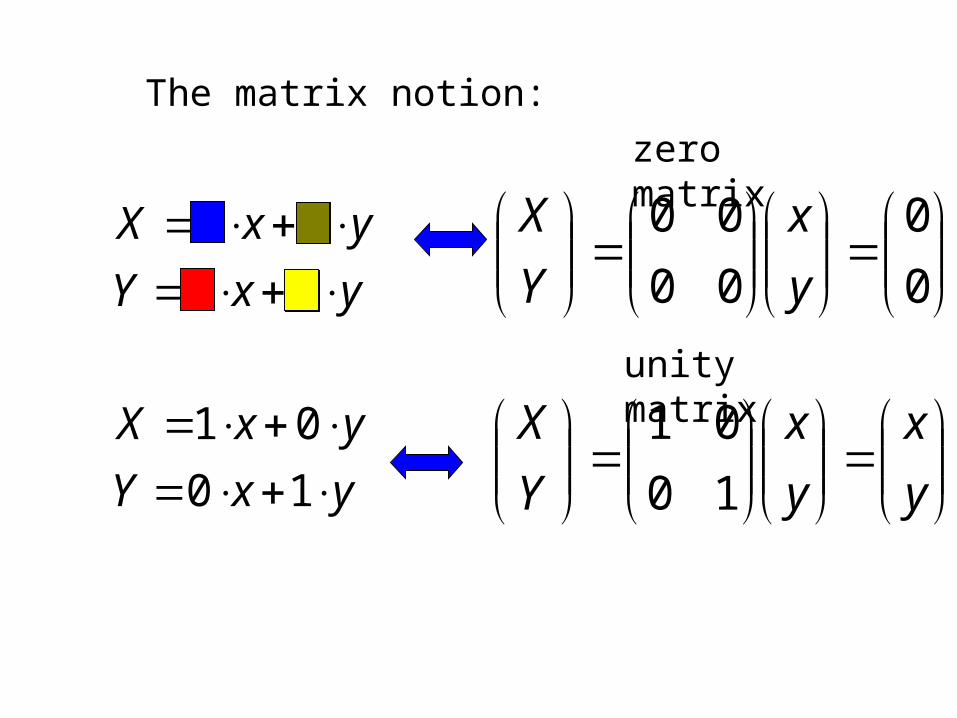
The function that takes every point to (0,0) : the zero function
The function that doesn’t do anything : the unity function
010
001
yxY
yxX
000
000
yxY
yxX
zero matrix
yxY
yxX
00
00
0
0
00
00
y
x
Y
X
yxY
yxX
10
01
y
x
y
x
Y
X
10
01
The matrix notion:
unity matrix

•Every linear function 2-D to 2-D can be written by a 2x2 matrix
•Every 2x2 matrix represent a linear function from 2-D to 2-D
cossin
sincos
yxY
yxX
y
x
Y
X
cossin
sincos
Another example: a rotation matrix
More examples: reflection, compression, stretching…

y
x
y
x
Y
X
cossin
sincos
Ф
In a rotation, the vector’s length remain the same

0
0
00
00
y
x
Y
X00
vV
The matrix notion:
y
x
y
x
Y
X
10
01vvIdV
???/ 1 vvvvId

Y
X
y
x
y
x
Y
X1
10
01
10
01
?1
Y
X
y
x
y
x
Y
X
Matrix math: only square matrices can be inverted, and not even all of them
zero matrix inverse?
?00
00
00
001
Y
X
y
x
y
x
Y
X
unity matrix inverse?

A vector which is only scaled by a specific matrix operation is called an eigenvector. The scaling factor is called an eigenvalue .
y
x
vvA

Anyway, one thing remains: the reversibility of a matrix depends on its eigenvalues. Invertible matrix no zero eigenvalues, λ≠0.
What is the physical meaning of the eigenvectors/ values?
For every use of matrices there is a different meaning. We will see an example.

A major task of engineering:
make the data easy on the eyes[1]
• Biology example: cell signaling.
• Many signals, many observations = big matrix, big mess
• Transform this matrix into something we can look at, by choosing the best x and y axes
[1] Kevin A. Janes and Michael B. Yaffe, Data-driven modeling of signal-transduction networks, Nature Reviews Molecular Cell Biology 7, 820-828 (November 2006)
“The paradox for systems biology is that these large data sets by themselves often bring more confusion than understanding” [1]

The idea: arrange the rows and columns of the matrix in a way that reveals biological meaning
The example: measure the co-variance (how 2 cell signals change “together”), to create a matrix:
•This matrix represent a linear function
•The matrix work on a vector of cell signals
•For the eigenvectors, the matrix just change the vector size (multiply by the eigenvalue)
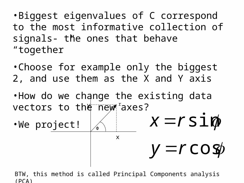
•Biggest eigenvalues of C correspond to the most informative collection of signals- the ones that behave “together”
•Choose for example only the biggest 2, and use them as the X and Y axis
•How do we change the existing data vectors to the new axes?
•We project!y
x
Ф
r
cos
sin
ry
rx
BTW, this method is called Principal Components analysis (PCA)

Another use of matrices: advance in time
0
1
1
0
01
10)2(
1
0
0
1
01
10)(
0
1
01
10,
tv
tv
v
AxYyX
)()( tvAttv
exampley
x

Use of matrices: propagator function- advance in time
1
1
1
1
01
10)(
1
1
1
1
01
10)(
tv
tv
y
x45○
What is the eigenvalues of the eigenvectors?
The 2 eigenvectors can be thought of 2 modes of movement in the space- one motionless, the other ‘jumps’ 180 degrees.
And if we build a new vector, a combination of the 2 eigenvectors?

Combination of eigenvector with non-eigenvector
1
2
2
1
01
10)2(
2
1
1
2
01
10)(
1
2
0
1
1
1
tv
tv
v
y
x
What will happen if ?
0
2
12
10
A

Summary:
When the matrix is a propagator the eigenvectors with eigenvalue 1 are the stable states (along side 0)
When the eigenvalues are less than one the system will decay to 0
When the eigenvalues are higher than one the system will grow and grow…
What if we want to check the system state after many time steps?
n
tnv
tv
3.07.0
7.03.0)(
3.07.0
7.03.0
3.07.0
7.03.0
3.07.0
7.03.0)2(
2

How do we calculate the matrix power?
Using the eigenvectors, we can write the matrix as a multiplication of 3 matrices:
5.05.0
5.05.0
4.00
01
5.05.0
5.05.0
3.07.0
7.03.0
10
01
5.05.0
5.05.0
5.05.0
5.05.0
5.05.0
5.05.0
4.00
01
5.05.0
5.05.0
3.07.0
7.03.0
5.0
5.02,
5.0
5.01
n
nn
vv

What can such matrix mean?
- Ligand / receptor binding state, and next state probabilities[2]
Capture state
Free state
0.7
0.3
0.7
0.3
)0,(
)0,(
7.03.0
3.07.0
),(
),(
freeP
captureP
tfreeP
tcaptureP
[2], A. Hassibi, S. Zahedi, R. Navid, R. W. Dutton, and T. H. Lee, Biological Shot-noise and Quantum-Limited SNR in Affinity-Based Biosensor, Journal of Applied Physics, 97-1, (2005).

?1
0
7.03.0
3.07.0
),(
),(
58.0
42.0
1
0
7.03.0
3.07.0
7.03.0
3.07.0
)2,(
)2,(
7.0
3.0
1
0
7.03.0
3.07.0
),(
),(
freeP
captureP
tfreeP
tcaptureP
tfreeP
tcaptureP
For example, assume all ligands are free at time zero:
As only the eigenvector of 1 survives (0.4 mode goes down to zero), we will be left with a uniform probability of (½, ½)- half of the ligand molecules are captured and half are free at steady state

Another example: Evolutionary Biology and genetics“evolutionary biology rests firmly on a foundation of linear algebra”[3]
•Observations are made on the covariance matrix of traits denoted G
•A genetic constraint is a factor that effects the direction of evolution or prevents adaptation
•Genetic correlation that show no variance in a direction of selection will constrain the evolution in that direction. How can we see it in the matrix?
[3], M. W. Blows, A tale of two matrices: multivariate approaches in evolutionary biology, Journal of Evolutionary
Biology , Volume 20 Issue 1 Page 1-8, (January 2007)
A zero eigenvalue