a general 3d non-stationary wireless channel model for 5g

IEEE TRANSACTIONS ON WIRELESS COMMUNICATIONS, VOL. 20, NO. 5, MAY 2021 3211

A General 3D Non-Stationary Wireless ChannelModel for 5G and Beyond

Ji Bian, Member, IEEE, Cheng-Xiang Wang , Fellow, IEEE, Xiqi Gao , Fellow, IEEE,

Xiaohu You , Fellow, IEEE, and Minggao Zhang

Abstract— In this paper, a novel three-dimensional (3D)non-stationary geometry-based stochastic model (GBSM) for thefifth generation (5G) and beyond 5G (B5G) systems is proposed.The proposed B5G channel model (B5GCM) is designed tocapture various channel characteristics in (B)5G systems such asspace-time-frequency (STF) non-stationarity, spherical wavefront(SWF), high delay resolution, time-variant velocities and direc-tions of motion of the transmitter, receiver, and scatterers, spatialconsistency, etc. By combining different channel properties into ageneral channel model framework, the proposed B5GCM is ableto be applied to multiple frequency bands and multiple scenar-ios, including massive multiple-input multiple-output (MIMO),vehicle-to-vehicle (V2V), high-speed train (HST), and millimeterwave-terahertz (mmWave-THz) communication scenarios. Keystatistics of the proposed B5GCM are obtained and comparedwith those of standard 5G channel models and correspondingmeasurement data, showing the generalization and usefulness ofthe proposed model.

Index Terms— 3D space-time-frequency non-stationary GBSM,massive MIMO, mmWave-THz, high-mobility, multi-mobilitycommunications.

Manuscript received January 31, 2020; revised August 11, 2020 andDecember 12, 2020; accepted December 23, 2020. Date of publicationJanuary 8, 2021; date of current version May 10, 2021. This work wassupported in part by the National Key Research and Development Program ofChina under Grant 2018YFB1801101, in part by the National NaturalScience Foundation of China (NSFC) under Grant 61960206006, in part bythe Shandong Provincial Natural Science Foundation for Young Scholars ofChina under Grant ZR2020QF001, in part by the Taishan Scholar Program ofShandong Province, in part by the Frontiers Science Center for Mobile Infor-mation Communication and Security, in part by the High Level Innovation andEntrepreneurial Research Team Program in Jiangsu, in part by the High LevelInnovation and Entrepreneurial Talent Introduction Program in Jiangsu, in partby the Research Fund of National Mobile Communications Research Labora-tory, Southeast University under Grant 2020B01, in part by the FundamentalResearch Funds for the Central Universities under Grant 2242020R30001,and in part by the EU H2020 RISE TESTBED2 Project under Grant 872172.The associate editor coordinating the review of this article and approving itfor publication was T. G. Pratt. (Corresponding author: Cheng-Xiang Wang.)

Ji Bian is with the School of Information Science and Engineering, Shan-dong Normal University, Jinan 250358, China (e-mail: [email protected]).

Cheng-Xiang Wang, Xiqi Gao, and Xiaohu You are with the NationalMobile Communications Research Laboratory, School of Information Scienceand Engineering, Southeast University, Nanjing 210096, China, and alsowith the Purple Mountain Laboratories, Nanjing 211111, China (e-mail:[email protected]; [email protected]; [email protected]).

Minggao Zhang is with the Shandong Provincial Key Laboratory ofWireless Communication Technologies, School of Information Science andEngineering, Shandong University, Qingdao 266237, China (e-mail: [email protected]).

Color versions of one or more figures in this article are available athttps://doi.org/10.1109/TWC.2020.3047973.

Digital Object Identifier 10.1109/TWC.2020.3047973

I. INTRODUCTION

THE growing requirement of high data rate transmis-sion caused by the popularization of wireless services

and applications results in a spectrum crisis in current sub-6 GHz bands. To address this challenge, the fifth genera-tion (5G)/beyond 5G (B5G) wireless communication systemswill transmit data using millimeter wave (mmWave)/terahertz(THz) bands in multiple propagation scenarios, e.g., high-speed train (HST) and vehicle-to-vehicle (V2V) scenarios [1].The short wavelengths of mmWave-THz bands make it pos-sible to deploy large antenna arrays with high beamforminggains that can overcome the severe path loss [2]. Revolutionarytechnologies employed in 5G and B5G wireless communica-tion systems such as massive multiple-input multiple-output(MIMO), HST, V2V, and mmWave-THz communicationsintroduce new channel properties, such as spherical wavefront(SWF), spatial non-stationarity, oxygen absorption, etc. Thesein turn will set new requirements to standard (B)5G channelmodels, i.e., supporting multiple frequency bands and multiplescenarios, as follows [3], [4]:

1) Multiple frequency bands, covering sub-6 GHz,mmWave, and THz bands;

2) Large bandwidth, e.g., 0.5–4 GHz for mmWave bandsand 10 GHz for THz bands;

3) Massive MIMO scenarios: spatial non-stationarity andSWF;

4) HST scenarios: temporal non-stationarity includingparameters’ drifting and clusters’ appearance and dis-appearance over time;

5) V2V scenarios: temporal non-stationarity and multi-mobility, i.e., the transmitter (Tx), receiver (Rx), andscatterers may move with time-variant velocities andheading directions;

6) Three-dimensional (3D) scenarios, especially for indoorand outdoor small cell scenarios;

7) Spatial consistency scenarios, i.e., closely located linksexperience similar channel statistical properties.

In massive MIMO communications, the large arrays makethe channel spatially non-stationary, which means channelparameters and statistical properties vary along array axis [4].For example, measurement results in [5] and [6] showedthat the angles of multipath components (MPCs) drift acrossthe array, justifying the SWF assumption of the channel.This implies that travel distances from every Tx antenna

1536-1276 © 2021 IEEE. Personal use is permitted, but republication/redistribution requires IEEE permission.See https://www.ieee.org/publications/rights/index.html for more information.

Authorized licensed use limited to: Southeast University. Downloaded on May 10,2021 at 15:09:24 UTC from IEEE Xplore. Restrictions apply.

https://orcid.org/0000-0002-9729-9592

https://orcid.org/0000-0001-9107-6593

https://orcid.org/0000-0002-0809-8511

3212 IEEE TRANSACTIONS ON WIRELESS COMMUNICATIONS, VOL. 20, NO. 5, MAY 2021

element to the Rx/scatterers at each time instant (if temporalnon-stationarity is considered) have to be calculated,resulting in high model complexity [7]–[9]. Measurements in[10] and [11] revealed that the mean delay, delay spread, andcluster power can vary across the large array. Here, a clusteris a group of MPCs having similar properties in delay, power,and angles. Note that the cluster power variation over arrayhas not been considered in most massive MIMO channelmodels [7]–[9]. Furthermore, when large arrays are adopted,clusters illustrate a partially visible property. Some clustersare visible over the whole array, while other clusters can onlyinteract with part of the array [6], [12]. In [13] and [14],the partially visibility of clusters was modeled by introducingthe concept of “BS-visibility region (VR)”. Other researchessuch as [7] and [15] described the partial visibility of clustersusing birth-death or Markov processes. In general, how toefficiently and synthetically model the non-stationarities inthe time and space domains has to be solved in the (B)5Gchannel modeling.

In V2V channels, channel parameters and statistical proper-ties are time-varying caused by the motions of the Tx, Rx, andscatterers [16]. Besides, channel measurements showed thatclusters of V2V channels can exhibit a birth-death behavior,i.e., appear, exist for a time period, and then disappear [4].Large numbers of V2V channel models were designed as puregeometry-based stochastic model (pure-GBSM) [17], [18].The scatterers of those models were assumed to be locatedon regular shapes, which are less versatile than those ofthe WINNER/3GPP models [19], [20]. More realistic V2Vchannel models, e.g., [21] and [22], were developed basedon channel measurements. However, the motions of scattererswere neglected. Furthermore, the variations of velocity andtrajectory of the Tx/Rx were not taken into account.

The HST channels share some similar properties withV2V channels, e.g., large Doppler shifts and temporal non-stationarity. Widely used standard channel models, e.g.,WINNER II [23] and IMT-Advanced channel models [24] canbe applied to HST scenarios where the velocity of train canbe up to 350 km/h. However, those models were developedbased on temporal wide-sense stationary (WSS) assumption.The HST channel model in [25] was developed based onIMT-Advanced channel model [24] by taking into accountthe time-varying angles and cluster evolution. More generalHST channel model was proposed in [26], which extended theelliptical model by assuming velocity and moving directionvariations. However, the above-mentioned models are two-dimensional (2D) and can only be applied to the scenarioswhere the transceiver and scatterers are sufficiently far away.In [27], a 3D non-stationary HST channel model was pro-posed, which can only be used in tunnel scenarios. In [28],a tapped delay line model was presented for various HSTscenarios, e.g., viaduct and cutting. The fidelity of the modelrelies on the model parameters obtained from ray-tracing,resulting in high computation complexity.

For the mmWave-THz communications, high frequenciesresult in large path loss and render the mmWave-THz propaga-tion susceptible to blockage effects and oxygen absorption [3].Compared with sub-6 GHz bands, the mmWave-THz channels

are sparser [29]. High delay resolution is required in channelmodeling due to the large bandwidth. Rays within a clustercan have different time of arrival, leading to unequal raypowers [20]. Besides, as the relative bandwidth increases,the channel becomes non-stationary in the frequency domain,which means the uncorrelated scattering (US) assumptionmay not be fulfilled [30]. Furthermore, directional anten-nas are often deployed to overcome the high attenuation atmmWave-THz frequency bands. In [31], a 2D mmWave V2Vchannel model was proposed. The influence of directionalantennas was represented by eliminating the clusters outsidethe main lobe of antenna patterns. MmWave-THz channelmodels should faithfully recreate the spatial, temporal and fre-quency characteristics for every single ray, such as the modelsin [32] and [33]. However, those models are oversimplified andcannot support time evolution since the model parameters aretime-invariant.

Apart from modeling channel characteristics in variousscenarios, another challenge for (B)5G channel modeling liesin how to combine those channel characteristics into a generalmodeling framework. Standard channel models aim to solvethis problem. In order to achieve smooth time evolution,the COST 2100 channel model introduces the “VR”, whichindicates whether a cluster can be “seen” from the mobilestation (MS). The clusters are considered to physically existin the environments and do not belong to a specific link. Thus,closely located links can experience similar environments,justifying the spatial consistency of the model. However,the COST 2100 channel model can only support sub-6 GHzbands. Furthermore, massive MIMO and dual-mobility werenot supported. The QuaDriGa [34] channel model is extendedfrom 3GPP TR36.873 [35] and support frequencies over0.45–100 GHz. The model parameters were generated basedon spatially correlated random variables. Links located nearbyshare similar channel parameters and therefore supports spatialconsistency. However, the complexities of those models arerelatively high and the dual-mobility was neglected. The3GPP TR38.901 [20] channel model extended the 3GPPTR36.873 by supporting the frequencies over 0.5–100 GHz.The oxygen absorption and blockage effect for the mmWavebands were modeled. However, for high-mobility scenarios,the clusters fade in and fade out were not considered, whichresults in limited ability for capturing time non-stationarity.Besides, the dual-mobility and SWF cannot be supported. Notethat all the above-mentioned standard channel models assumedconstant cluster power for different antenna elements and didnot consider scatterers movements.

A GBSM called more general 5G channel model(MG5GCM) aims at capturing various channel propertiesin 5G systems [9]. Based on a general model framework,the model can support various communication scenarios.However, the azimuth angles, elevation angles, and traveldistances between Tx/Rx and scatterers were generated inde-pendently. The model can only evolve along the time andarray axes, and neglected the non-stationary properties in thefrequency domain. The locations of scatterers were implicitlydetermined by the angles and delays, which makes the modeldifficult to achieve spatial consistency. Besides, it neglected


BIAN et al.: GENERAL 3D NON-STATIONARY WIRELESS CHANNEL MODEL FOR 5G AND BEYOND 3213

the dynamic velocity and direction of motion of the Tx, Rx,and scatterers.

Through above analysis, we find that none of these standardchannel models can meet all the 5G channel modeling require-ments. Considering these research gaps, this paper proposesa general (B)5G channel model (B5GCM) towards multiplefrequency bands and multiple scenarios. The contributions ofthis paper are listed as follows:

1) The system functions, correlation functions (CFs),and power spectrum densities (PSDs) of space-time-frequency (STF) stationary and non-stationary channelsare presented. A general 3D STF non-stationary ultra-wideband channel model is developed. By setting appro-priate channel model parameters, the model can supportmultiple frequency bands and multiple scenarios.

2) A highly accurate approximate expression of the 3DSWF is proposed, which is more scalable and efficientthan the traditional modeling method and can capturespatial and temporal channel non-stationarities. Thecluster evolutions along the time and array axes arejointly considered and simulated using a unified birth-death process. The smooth power variation over the largearrays is modeled by a 2D spatial lognormal process.

3) The novel ellipsoid Gaussian scattering distribution isproposed which can jointly describe the azimuth angles,elevation angles, and distances from the Tx(Rx) to thefirst(last)-bounce scatterers. By tracking the locations ofthe Tx, Rx, and scatterers, the spatial consistency of thechannel is supported.

4) The proposed B5GCM takes into account a multi-mobility communication environment, where the Tx, Rx,and scatterers can change their velocities and movingdirections.

5) Key statistics including local STF-CF, local spatial-Doppler PSD, local Doppler spread, and array coherencedistance are derived and compared with standard 5Gchannel models and the corresponding measurementdata.

The remainder of this paper is organized as follows.In Section II, the system, correlation, and spectrum functionsof the STF non-stationary channel model are presented. Theproposed B5GCM is described in Section III. Statistics of theB5GCM are investigated in Section IV. In Section V, numericaland simulation results are provided and discussed. Conclusionsare drawn in Section VI.

II. SYSTEM FUNCTIONS, CFS, AND PSDsOF SPACE, TIME, AND FREQUENCY

NON-STATIONARY CHANNELS

Wireless channels can be described through system func-tions, CFs, and PSDs. The time-frequency selectivity anddelay-Doppler dispersion of wireless channels have been stud-ied in [36] and [37]. In this paper, the non-stationarity ofchannels in the space domain is considered, which is anessential property for massive MIMO channels. The basicfunction characterizing the wireless channel is the space andtime-varying channel impulse response (CIR) h(r, t, τ). It is

modeled as a stochastic process on space r, time t, and delay τ .Note that the space domain indicates the region where ris confined along a linear antenna array. Taking the Fouriertransform of h(r, t, τ) with respect to (w.r.t.) τ results in space-and time-varying transfer function, which is given by

H(r, t, f) =∫

h(r, t, τ)e−j2πτfdτ. (1)

The space and time-varying transfer function characterizes thespace, time, and frequency selectivity of wireless channels.Moreover, taking the Fourier transform of h(r, t, τ) w.r.t. rand t results in the spatial-Doppler Doppler delay spreadfunction, i.e.,

s(�, ν, τ) =∫∫

h(r, t, τ)e−j2π(r�λ−1+tν)drdt. (2)

Here, λ is the wavelength, � is the spatial-Doppler frequencyvariable defined as � = Ω · Ω̃, where Ω is an angle unitvector of the departure/arrival waves, Ω̃ indicates the antennaarray orientation [38]. The space variable r and the spatial-Doppler variable � are Fourier transformation pair. Since rhas a distance unit, the unit of � must be its reciprocal,i.e., per normalized distance (w.r.t. λ). The terminology �stems from the fact that Ω · Ω̃ is the Doppler shift of awave with direction Ω impinging on an antenna which moveswith λ m/s in direction Ω̃. The spatial-Doppler Dopplerdelay spread function characterizes the dispersions of wirelesschannels in the spatial-Doppler frequency, Doppler frequency,and delay domains. Similarly, by taking the Fourier transformof h(r, t, τ) w.r.t. r, t, and/or τ , totally eight system functionscan be obtained [39]. Based on those formulas, e.g., h(r, t, τ),H(r, t, f), and s(�, ν, τ), the six-dimensional (6D) CFs arederived as

Rh(r, t, τ ; Δr, Δt, Δτ)= E{h(r, t, τ)h∗(r − Δr, t − Δt, τ − Δτ)} (3)

RH(r, t, f ; Δr, Δt, Δf)= E{H(r, t, f)H∗(r − Δr, t − Δt, f − Δf)} (4)

Rs(�, ν, τ ; Δ�, Δν, Δτ)= E{s(�, ν, τ)s∗(� − Δ�, ν − Δν, τ − Δτ)} (5)

where E{·} indicates ensemble average and (·)∗ stands forcomplex conjugation, Δr, Δt, and Δf are space, time, andfrequency lags, respectively. A channel is STF non-stationaryif RH(r, t, f ; Δr, Δt, Δf) is not only a function of Δr, Δt,and Δf , but also relies on r, t, and f . Its simplification,i.e., WSS over r, t, and f is widely used in the existing channelmodels. However, it is valid only if the channel satisfies certainconditions. For example, when the distance from the Tx to theRx (or a cluster) is less than the Rayleigh distance, i.e., 2L2

λ ,where L denotes the aperture size of the antenna array andλ is the carrier wavelength, the spatial WSS condition is ful-filled [8]. The temporal WSS assumption is valid as long as thechannel stationary interval is larger than the observation time.Finally, when the relative bandwidth of the channel is small(typically less than 20% of the carrier frequency), the channelbecomes WSS in the frequency domain. Considering the STF



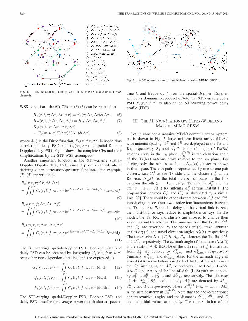
Fig. 1. The relationship among CFs for STF-WSS and STF-non-WSSchannels.

WSS conditions, the 6D CFs in (3)-(5) can be reduced to

Rh(r, t, τ ; Δr, Δt, Δτ) = Sh(τ ; Δr, Δt)δ(Δτ) (6)

RH(r, t, f ; Δr, Δt, Δf) = RH(Δr, Δt, Δf) (7)

Rs(�, ν, τ ; Δ�, Δν, Δτ)= Cs(�, ν, τ)δ(Δ�)δ(Δν)δ(Δτ) (8)

where δ(·) is the Dirac function, Sh(τ ; Δr, Δt) is space timecorrelation, delay PSD and Cs(�, ν, τ) is spatial-DopplerDoppler delay PSD. Fig. 1 shows the complete CFs and theirsimplifications by the STF WSS assumption.

Another important function is the STF-varying spatial-Doppler Doppler delay PSD, since it plays a central role inderiving other correlation/spectrum functions. For example,(3)–(5) are written as

Rh(r, t, τ ; Δr, Δt, Δτ)

=∫∫∫

Cs(r, t, f ; �, ν, τ)ej2π(�Δrλ−1+νΔt+fΔτ)d�dνdf

(9)

RH(r, t, f ; Δr, Δt, Δf)

=∫∫∫

Cs(r, t, f ; �, ν, τ)ej2π(�Δrλ−1+νΔt−τΔf)d�dνdτ

(10)

Rs(�, ν, τ ; Δ�, Δν, Δτ)

=∫∫∫

Cs(r, t, f ; �, ν, τ)ej2π(−Δ�rλ−1−Δνt+Δτf)drdtdf.

(11)

The STF-varying spatial-Doppler PSD, Doppler PSD, anddelay PSD can be obtained by integrating Cs(r, t, f ; �, ν, τ)over other two dispersion domains, and are expressed as

Gs(r, t, f ; �) =∫∫

Cs(r, t, f ; �, ν, τ)dνdτ (12)

Qs(r, t, f ; ν) =∫∫

Cs(r, t, f ; �, ν, τ)d�dτ (13)

Ps(r, t, f ; τ) =∫∫

Cs(r, t, f ; �, ν, τ)d�dν. (14)

The STF-varying spatial-Doppler PSD, Doppler PSD, anddelay PSD describe the average power distribution at space r,

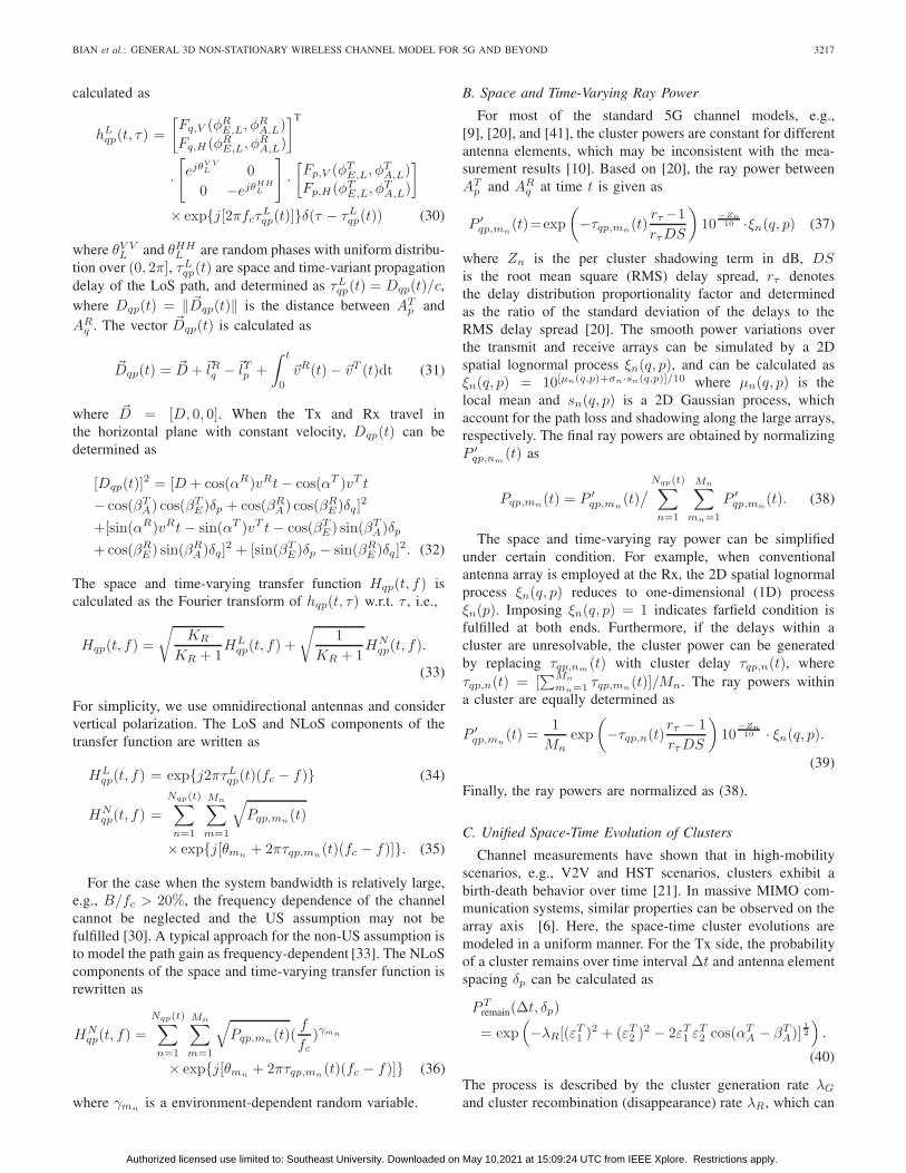
Fig. 2. A 3D non-stationary ultra-wideband massive MIMO GBSM.

time t, and frequency f over the spatial-Doppler, Doppler,and delay domains, respectively. Note that STF-varying delayPSD Ps(r, t, f ; τ) is also called STF-varying power delayprofile (PDP).

III. THE 3D NON-STATIONARY ULTRA-WIDEBAND

MASSIVE MIMO GBSM

Let us consider a massive MIMO communication system.As is shown in Fig. 2, large uniform linear arrays (ULAs)with antenna spacings δT and δR are deployed at the Tx andRx, respectively. Symbol β

T (R)A is the tilt angle of Tx(Rx)

antenna array in the xy plane, βT (R)E is the elevation angle

of the Tx(Rx) antenna array relative to the xy plane. Forclarity, only the nth (n = 1, . . . , Nqp(t)) cluster is shownin this figure. The nth path is represented by one-to-one pairclusters, i.e., CA

n at the Tx side and the cluster CZn at the

Rx side. Nqp(t) is the total number of paths in the linkbetween the pth (p = 1, . . . , MT ) Tx antenna AT

p and theqth (q = 1, . . . , MR) Rx antenna AR

q at time instant t. Thepropagation between CA

n and CZn is abstracted by a virtual

link [23]. There could be other clusters between CAn and CZ

n ,introducing more than two reflections/interactions betweenthe Tx and Rx. When the delay of the virtual link is zero,the multi-bounce rays reduce to single-bounce rays. In thismodel, the Tx, Rx, and clusters are allowed to change theirvelocities and trajectories. The movements of the Tx, Rx, CA

n ,and CZ

n are described by the speeds vX(t), travel azimuthangles αX

A (t), and travel elevation angles αXE (t), respectively.

The superscript X ∈ {T, R, An, Zn} denotes the Tx, Rx, CAn ,

and CZn , respectively. The azimuth angle of departure (AAoD)

and elevation AoD (EAoD) of the mth ray in CAn transmitted

from AT1 are denoted by φT

A,mnand φT

E,mn, respectively.

Similarly, φRA,mn

and φRE,mn

stand for the azimuth angle ofarrival (AAoA) and elevation AoA (EAoA) of the mth ray inthe CZ

n impinging on AR1 , respectively. The EAoD, EAoA,

AAoD, and AAoA of the line-of-sight (LoS) path are denotedby φT

E,L, φRE,L, φT

A,L, and φRA,L, respectively. The distances

of AT1 –SA

mn, SZ

mn–AR

1 , and AT1 –AR

1 are denoted by dTmn

,dR

mn, and D, respectively, where S

A(Z)mn (mn = 1, . . . , Mn)

is the mth scatterer in CA(Z)n . Note that the above-mentioned

departure/arrival angles and the distances dTmn

, dRmn

, and Dare the initial values at time t0. The time-variation of the



TABLE I

SUMMARY OF KEY PARAMETER DEFINITIONS

proposed model is described in the remainder of this section.The parameters in Fig. 2 are defined in Table I.

A. Channel Impulse Response

Considering small-scale fading, path loss, shadowing, oxy-gen absorption, and blockage effect, the complete channelmatrix is given by H = [PL · SH · BL · OL]

12 · Hs, where

PL denotes the path loss. Widely used path loss model canbe found in [40], which has been recommended as the pathloss model for 5G systems. SH denotes the shadowing andis modeled as lognormal random variables [40]. The blockageloss BL caused by humans and vehicles is taken from [3].The oxygen absorption loss OL for mmWave and THz com-munications can be found in [41] and [42], respectively. Notethat PL, SH , BL, and OL are in power level, which can betransformed into the corresponding dB values as 10 log10(α),where α ∈ {PL, SH, BL, OL}.

The small-scale fading is represented as a complex matrixHs = [hqp(t, τ)]MR×MT , where hqp(t, τ) is the CIR betweenAT

p and ARq and expressed as the summation of the LoS and

non-LoS (NLoS) components, i.e.,

hqp(t, τ) =√

KR

KR + 1hL

qp(t, τ) +√

1KR + 1

hNqp(t, τ) (15)

where KR is the K-factor. The NLoS components hNqp(t, τ)

can be written as

hNqp(t, τ)

=Nqp(t)∑n=1

Mn∑m=1

[Fq,V (φR

E,mn, φR

A,mn)

Fq,H(φRE,mn

, φRA,mn

)

]T

·[

ejθV Vmn

√μκ−1

mnejθV Hmn√

κ−1mnejθHV

mn√

μejθHHmn

][Fp,V (φT

E,mn, φT

A,mn)

Fp,H(φTE,mn

, φTA,mn

)

]

·√

Pqp,mn(t)ej2πfcτqp,mn (t) · δ(τ − τqp,mn(t)) (16)

where {·}T denotes transposition, fc is the carrier frequency,Fp(q),V and Fp(q),H are the antenna patterns of AT

p (ARq ) for

vertical and horizontal polarizations, respectively. Note thatthe proposed propagation channel model is designed to be

Fig. 3. The projection of the propagation between the Tx and SAmn

on thexy plane.

antenna independent, which means different antenna patternscan be applied without modifying the basic model framework.Symbol κmn stands for the cross polarization power ratio [20],μ is co-polar imbalance, θV V

mn, θV H

mn, θHV

mn, and θHH

mnare initial

phases with uniform distribution over (0, 2π], Pqp,mn(t) andτqp,mn(t) are the powers and delays of the mth ray in the nthcluster between AT

p and ARq at time t, respectively. Consider-

ing large sizes of antenna array and high-mobility scenarios,the non-stationarities on time axis and array axis have to beconsidered. The number of clusters Nqp(t), the power of rayPqp,mn(t), and the propagation delay τqp,mn(t) are modeledas space and time-dependent. The propagation delay τqp,mn(t)is determined as

τqp,mn(t) = dqp,mn(t)/c + τ̃mn . (17)

Here, c denotes the speed of light, τ̃mn indicates the delayof the link between SA

mnand SZ

mn, and is modeled as τ̃mn =

d̃mn/c+τC,link, where d̃mn is the distance of SAmn

–SZmn

, τC,link

is a non-negative variable randomly generated according toexponential distribution [43]. The travel distance dqp,mn(t) isexpressed as dqp,mn(t) = ‖ dT

p,mn(t)‖+‖ dR

mn,q(t)‖, where ‖·‖stands for the Frobenius norm, dT

p,mn(t) and dR

mn,q(t) are thevector from AT

p to SAmn

and the vector from ARq to SZ

mnat

time t, respectively. Since the symmetry of the propagation,only the first-bounce propagation between AT

p and SAmn

isdescribed. For the sake of clarity, Fig. 3 shows the projection



of propagation between the Tx and SAmn

on the xy plane.Considering the time-varying speeds and trajectories of theTx and CA

n , dTp,mn

(t) is calculated as

dTp,mn

(t) = dTmn

− [ lTp +∫ t

0

vT (t) − vAn(t)dt] (18)

where

dTmn

= dTmn

⎡⎢⎣cos(φT

E,mn) cos(φT

A,mn)

cos(φTE,mn

) sin(φTA,mn

)sin(φT

E,mn)

⎤⎥⎦

T

(19)

lTp = δp

⎡⎢⎣cos(βT

E) cos(βTA)

cos(βTE) sin(βT

A)sin(βT

E)]

⎤⎥⎦

T

(20)

vT (t) = vT (t)

⎡⎢⎣cos

(αT

E(t))cos

(αT

A(t))

cos(αT

E(t))sin(αT

A(t))sin

(αT

E(t))

⎤⎥⎦

T

(21)

vAn(t) = vAn(t)

⎡⎢⎣cos(αAn

E (t)) cos(αAn

A (t))cos(αAn

E (t)) sin(αAn

A (t))sin(αAn

E (t))]

⎤⎥⎦

T

. (22)

Here δp = (p − 1)δT , indicates the distance of ATp –AT

1 .For most cases, the Tx, Rx, and scatterers move in the

xy plane. For conciseness, we use vT = ‖ vT − vAn‖ andαT = arg{ vT − vAn} to denote the relative speed and angleof motion of the Tx w.r.t. CA

n , respectively, where arg{·}calculates the argument of a 2D vector. When the Tx, Rx andclusters move with constant speeds along straight trajectories,by extending the 2D parabolic wavefront [44] into 3D timenon-stationary case, travel distance dT

p,mn(t) = ‖ dT

p,mn(t)‖ is

approximated as

dTp,mn

(t) ≈ dTmn

− cos(ωTp )vT t − cos(ϑT )δp︸︷︷︸

WSS PWF approximation

+sin2(ϑT )δ2

p

2dTmn︸︷︷︸

SWF term

+sin2(ωT

p )(vT t)2

2[dTmn

− cos(ϑT )δp]︸︷︷︸non-WSS term

(23)

where ϑT is the angle between the the transmit antenna arrayand the mth ray in the nth cluster transmitted from AT

1 , andis calculated as

cos(ϑT ) = cos(φTE,mn

) cos(βTE) cos(βT

A − φTA,mn

)

+ sin(φTE,mn

) sin(βTE). (24)

In (23), ωTp stands for the angle from moving direction of the

Tx to the mth ray of the nth cluster transmitted from ATp , and

can be determined as (25), shown at the bottom of the page.Equation (23) gives an efficient and scalable approach for

modeling the 3D SWF under time non-stationary assumption.The first term in (23) gives the travel distance of AT

p –SAmn

link based on plane wavefront (PWF) and temporal WSSassumptions. The second and third terms account for the non-stationary properties of the channel in the space and timedomains, respectively. Under certain conditions, the traveldistance in (23) can be further simplified.

1) Case I: Non-WSS & PWF: When small antenna arraysare used, i.e., δp � dT

mn, the angle ωT

p becomes constant fordifferent antenna elements and (25) reduces to

cos(ωT ) = cos(αT − φTA,m) cos(φT

E,m). (26)

Note that the subscript “p” has been omitted for convenience.The SWF term in (23) tends to zero and dT

p,mn(t) reduces to

dTp,mn

(t) ≈ dTmn

− cos(ωT )vT t − cos(ϑT )δp

+sin2(ωT )(vT t)2

2[dTmn

− cos(ϑT )δp]. (27)

2) Case II: WSS & SWF: For slow-moving scenar-ios or short time periods, i.e. vT t � dT

mn, the non-WSS term

in (23) tends to zero, which makes the model stationary overthe time. The travel distance in (23) reduces to

dTp,mn

(t) ≈ dTmn

− cos(ωTp )vT t − cos(ϑT )δp +

sin2(ϑT )δ2p

2dTmn

.

(28)

3) Case III: WSS & PWF: When both time WSS and PWFconditions are fulfilled. The angle ωT

p is simplified accordingto (26). The travel distance in (23) reduces to a fundamentalexpression, which can be found in most of the existing channelmodels as [19], [23], [24], [35]

dTp,mn

(t) ≈ dTmn

− cos(ωT )vT t − cos(ϑT )δp. (29)

For the Rx side, dRmn,q(t), ϑR, and ωR

q are obtained byreplacing the superscript “T ” and subscript “p” with “R”and “q” in (18)–(29), respectively. Here, we briefly discussthe influence of the Doppler shifts on the proposed model.In (16) the phase rotation associated with time-varying traveldistance is given as ϕqp,mn(t) = 2πfcτqp,mn(t), and isdecomposed as ϕqp,mn(t) = 2πfc(‖ dT

p,mn(t)+ dR

q,mn(t)‖/c+

τ̃mn). The Doppler shift can be estimated by fmn(t) =dϕqp,mn(t)

dt and is time-varying. Considering the WSS & SWFcase in (28), the phase rotation can be further expressed asϕqp,mn(t) = 2π

λ

(dT

p,mn+ τ̃mnc + dT

mn,q

)− 2πt(fTmn

+ fRmn

),where dT

p,mn+ τ̃mnc + dT

mn,q accounts for the distance of

ATp –SA

mn–SZ

mn–AR

q link, fTmn

= vT

λ cosωTp and fR

mn=

vR

λ cosωRq are the Doppler shifts caused by the movement

of the Tx relative to CAn and the movement of the Rx relative

to CZn , respectively. Finally, the LoS component in (15) is

cos(ωTp ) =

dTmn

cos(αT − φTA,mn

) cos(φTE,mn

) − δp cos(αT − βTA) cos(βT

E)[(dT

mn)2 − 2dT

mnδp cos(ϑT ) + δ2

p]1/2. (25)



calculated as

hLqp(t, τ) =

[Fq,V (φR

E,L, φRA,L)

Fq,H(φRE,L, φR

A,L)

]T

·[ejθV V

L 00 −ejθHH

L

]·[Fp,V (φT

E,L, φTA,L)

Fp,H(φTE,L, φT

A,L)

]× exp{j[2πfcτ

Lqp(t)]}δ(τ − τL

qp(t)) (30)

where θV VL and θHH

L are random phases with uniform distribu-tion over (0, 2π], τL

qp(t) are space and time-variant propagationdelay of the LoS path, and determined as τL

qp(t) = Dqp(t)/c,where Dqp(t) = ‖ Dqp(t)‖ is the distance between AT

p andAR

q . The vector Dqp(t) is calculated as

Dqp(t) = D + lRq − lTp +∫ t

0

vR(t) − vT (t)dt (31)

where D = [D, 0, 0]. When the Tx and Rx travel inthe horizontal plane with constant velocity, Dqp(t) can bedetermined as

[Dqp(t)]2 = [D + cos(αR)vRt − cos(αT )vT t

− cos(βTA) cos(βT

E)δp + cos(βRA) cos(βR

E )δq]2

+[sin(αR)vRt − sin(αT )vT t − cos(βTE) sin(βT

A)δp

+ cos(βRE ) sin(βR

A)δq]2 + [sin(βTE)δp − sin(βR

E )δq]2. (32)

The space and time-varying transfer function Hqp(t, f) iscalculated as the Fourier transform of hqp(t, τ) w.r.t. τ , i.e.,

Hqp(t, f) =√

KR

KR + 1HL

qp(t, f) +√

1KR + 1

HNqp(t, f).

(33)

For simplicity, we use omnidirectional antennas and considervertical polarization. The LoS and NLoS components of thetransfer function are written as

HLqp(t, f) = exp{j2πτL

qp(t)(fc − f)} (34)

HNqp(t, f) =

Nqp(t)∑n=1

Mn∑m=1

√Pqp,mn(t)

× exp{j[θmn + 2πτqp,mn(t)(fc − f)]}. (35)

For the case when the system bandwidth is relatively large,e.g., B/fc > 20%, the frequency dependence of the channelcannot be neglected and the US assumption may not befulfilled [30]. A typical approach for the non-US assumption isto model the path gain as frequency-dependent [33]. The NLoScomponents of the space and time-varying transfer function isrewritten as

HNqp(t, f) =

Nqp(t)∑n=1

Mn∑m=1

√Pqp,mn(t)(

f

fc)γmn

× exp{j[θmn + 2πτqp,mn(t)(fc − f)]} (36)

where γmn is a environment-dependent random variable.

B. Space and Time-Varying Ray Power

For most of the standard 5G channel models, e.g.,[9], [20], and [41], the cluster powers are constant for differentantenna elements, which may be inconsistent with the mea-surement results [10]. Based on [20], the ray power betweenAT

p and ARq at time t is given as

P ′qp,mn

(t)=exp(−τqp,mn(t)

rτ −1rτDS

)10

−Zn10 ·ξn(q, p) (37)

where Zn is the per cluster shadowing term in dB, DSis the root mean square (RMS) delay spread, rτ denotesthe delay distribution proportionality factor and determinedas the ratio of the standard deviation of the delays to theRMS delay spread [20]. The smooth power variations overthe transmit and receive arrays can be simulated by a 2Dspatial lognormal process ξn(q, p), and can be calculated asξn(q, p) = 10[μn(q,p)+σn·sn(q,p)]/10 where μn(q, p) is thelocal mean and sn(q, p) is a 2D Gaussian process, whichaccount for the path loss and shadowing along the large arrays,respectively. The final ray powers are obtained by normalizingP ′

qp,nm(t) as

Pqp,mn(t) = P ′qp,mn

(t)/ Nqp(t)∑

n=1

Mn∑mn=1

P ′qp,mn

(t). (38)

The space and time-varying ray power can be simplifiedunder certain condition. For example, when conventionalantenna array is employed at the Rx, the 2D spatial lognormalprocess ξn(q, p) reduces to one-dimensional (1D) processξn(p). Imposing ξn(q, p) = 1 indicates farfield condition isfulfilled at both ends. Furthermore, if the delays within acluster are unresolvable, the cluster power can be generatedby replacing τqp,nm(t) with cluster delay τqp,n(t), whereτqp,n(t) = [

∑Mn

mn=1 τqp,mn(t)]/Mn. The ray powers withina cluster are equally determined as

P ′qp,mn

(t) =1

Mnexp

(−τqp,n(t)

rτ − 1rτ DS

)10

−Zn10 · ξn(q, p).

(39)

Finally, the ray powers are normalized as (38).

C. Unified Space-Time Evolution of Clusters

Channel measurements have shown that in high-mobilityscenarios, e.g., V2V and HST scenarios, clusters exhibit abirth-death behavior over time [21]. In massive MIMO com-munication systems, similar properties can be observed on thearray axis [6]. Here, the space-time cluster evolutions aremodeled in a uniform manner. For the Tx side, the probabilityof a cluster remains over time interval Δt and antenna elementspacing δp can be calculated as

PTremain(Δt, δp)

= exp(−λR[(εT

1 )2 + (εT2 )2 − 2εT

1 εT2 cos(αT

A − βTA)]

12

).

(40)

The process is described by the cluster generation rate λG

and cluster recombination (disappearance) rate λR, which can



be estimated as in [45]. Note that λG and λR are relatedto characteristics of scenarios and antenna patterns. In (40),εT1 = δp cos(βT

E)/DAc and εT

2 = vT Δt/DSc characterize the

position differences of transmit antenna element on array andtime axes, respectively. Symbols DA

c and DSc are scenario-

dependent correlation factors in the array and time domains,respectively. Typical values of DA

c and DSc such as 10 m and

30 m can be chosen, which are the same order of correlationdistances in [9], [20].

For the Rx side, the probability of a cluster exist overtime interval Δt and element spacing δq , i.e., PR

remain(Δt, δq),is calculated similarly. Since each antenna element has its ownobservable cluster set, only a cluster can be seen by at leastone Tx antenna and one Rx antenna, it can contribute to thereceived power. Therefore, the joint probability of a clusterexist over Δt and δq is calculated as

Premain(Δt, δp, δq) = PTremain(Δt, δp) · PR

remain(Δt, δq). (41)

The mean number of newly generated clusters is obtained by

E{Nnew} =λG

λR[1 − Premain(Δt, δp, δq)]. (42)

D. Ellipsoid Gaussian Scattering Distribution

The Gaussian scatter density model (GSDM) has widelybeen used in channel modeling for various communicationscenarios and validated by the measurement data [46], [47].In GSDM, the scatterers are gathered around their centerand usually modeled by certain shapes, e.g., discs in 2Dmodels and spheres in 3D models [48]. However, channelmeasurements indicate that the spatial dispersions of scattererswithin a cluster, which can be described by cluster angularspread (CAS), cluster elevation spread (CES), and clusterdelay spread (CDS), are usually unequal [3], [19]. Basedon the aforementioned assumption, the positions of scattererscentering on the origin of coordinates are modeled as

p(x′, y′, z′) =exp

(− x′2

2σ2DS

− y′2

2σ2AS

− z′22σ2

ES

)(2π)3/2

σDSσASσES

(43)

where σDS , σAS , and σES are the standard derivations of theGaussian distributions and characterize the CDS, CAS, andCES, respectively. The scatterers centering around the spher-ical coordinates (d, φE , φA) can be obtained by shifting theabove-mentioned cluster using the following transformation⎡⎣x

yz

⎤⎦ =

⎡⎣cos(φA) − sin(φA) 0

sin(φA) cos(φA) 00 0 1

⎤⎦

·⎡⎣cos(φE) 0 − sin(φE)

0 1 0sin(φE) 0 cos(φE)

⎤⎦ ·

⎡⎣x′ − d

y′

z′

⎤⎦ (44)

where d denotes the distance from the Tx/Rx to the centerof the cluster, φE and φA are the mean values of the ele-vation angles and azimuth angles of scatterers, respectively.Note that the orientation of the cluster toward the Tx/Rx isconstant through the aforementioned transformation, which

ensures the values of CDS, CAS, and CES remain unchanged.By substituting x = d cos(φE) cos(φA), y = d cos(φE)sin(φA), and z = d sin(φE) in to (44), after some manipula-tions, the angle distance joint distribution can be obtained as

p(d, φE , φA)

= |J(x′, y′, z′)| · p(x′, y′, z′)∣∣∣∣

x′ = d[cos(φE) cos(φE) cos(φA−φA) + sin(φE) sin(φE)]−d

y′ = d cos(φE) sin(φA−φA)z′ = d[sin(φE) cos(φE)−cos(φA−φA) cos(φE) sin(φE)]

(45)

where

J(x′, y′, z′) =

∣∣∣∣∣∣∣∣∣∣∣∣

∂x′

∂d

∂x′

∂φE

∂x′

∂φA

∂y′

∂d

∂y′

∂φE

∂y′

∂φA

∂z′

∂d

∂z′

∂φE

∂z′

∂φA

∣∣∣∣∣∣∣∣∣∣∣∣= −d2 cos(φE). (46)

By imposing τ̃mn = 0 in (17), the multi-bounce rays reduceto single-bounce rays. The delay angle joint distribution for thecluster can be obtained based on (45) by transform parameterd into τ , i.e.,

p(τ, φXE , φX

A ) = |J(dX)| · p(dX , φXE , φX

A ) (47)

where

dX =(τc)2 − D2

2τc − 2D cos(φXE ) cos(φX

A )(48)

J(dX) =ddX

dτ=

c[D2 + (τc)2 − 2Dcτ cos(φXE ) cos(φX

A )]2[τc − D cos(φX

E ) cos(φXA )]2

(49)

and X ∈ {T, R}. The angular parameters and travel distancesof the first- and last-bounce propagations becomes interdepen-dent. The relationship between them can be expressed as

tan(φTA)

=dR cos(φR

E) sin(φRA)

D + dR cos(φRE) cos(φR

A)(50)

tan(φTE)

=dR sin(φR

E){D2 + [dR cos(φR

E)]2 + 2D · dR cos(φRE) cos(φR

A)}1/2

(51)

dT = [D2 + (dR)2 + 2D · dR cos(φRE) sin(φR

A)]1/2. (52)

Note that the subscripts mn are omitted for clarity. Unlikethe WINNER/3GPP channel models [19], [20], [35], wherethe clusters are randomly generated for every link, in theproposed model, the clusters are assumed to physically existin the propagation environments. Thus, spatial consistency canbe achieved based on the locations of clusters. This makes itpossible to prediction channel state information (CSI) basedon the channel associated with nearby users or in the previoustime snapshots. For instance, in HST scenarios, different



Fig. 4. (a) Theoretical and (b) simulated ellipsoid Gaussian scatteringdistribution (σDS = 8, σAS = 10, σES = 6, d ∼ N (100, 10) m).

trains travel to the same location of the track will see sim-ilar environments and hence have similar channel behaviors.Channel can be estimated from the communication process oflast trains or nearby remote radio heads (RRHs) [49].

Fig. 4 shows the theoretical and simulated ellipsoidGaussian scattering distribution. The mean angles, i.e., φE

and φA are obtained from [20] in urban micro-cell scenario,NLoS case. The distances between the Tx and the centerof the first-bounce cluster follows a Gaussian distribution,i.e., N (100, 10) m. The simulated result is obtained usingMonte Carlo method and a total of 500 rays are generated.A good consistency between theoretical and simulated resultscan be observed.

By adjusting the model parameters or components, the pro-posed model can be applied to various scenarios. Let’s takemmWave-THz scenario as an example. The path loss, shad-owing, oxygen absorption, and blockage attenuation compo-nents can be replaced with those at mmWave-THz bands.The sparsity of MPCs can be represented by adjusting thenumber of clusters and the number of rays within a cluster.The remarkable birth-death behaviour of clusters over timeresulting from large propagation loss can be modeled byincreasing the cluster generation rate λG and recombinationrate λR. The antenna patterns in (16) can be replaced withthose of high-directional antennas, which are often used inmmWave-THz communications.

IV. STATISTICAL PROPERTIES

A. Local STF-CF

The local STF-CF between Hqp(t, f) and Hq̃p̃(t − Δt,f − Δf) is defined as

Rqp,q̃p̃(t, f ; Δr, Δt, Δf)=E{Hqp(t, f)H∗q̃p̃(t−Δt, f−Δf)}.

(53)

By substituting (33) into (53), the STF-CF is furtherwritten as

Rqp,q̃p̃(t, f ; Δr, Δt, Δf)

=KR

KR + 1RL

qp,q̃p̃(t, f ; Δr, Δt, Δf)

+1

KR + 1

Nqp(t)∑n=1

RNqp,q̃p̃,n(t, f ; Δr, Δt, Δf) (54)

where the LoS and NLoS components of the STF-CF can beobtained as

RLqp,qp̃(t, f ; Δr, Δt, Δf)

= [PLqp(t)PL

q̃p̃(t − Δt)]12

×ej 2π(fc−f)λfc

[dLqp(t)−dL

q̃p̃(t−Δt)]−j 2πΔfλfc

dLq̃p̃(t−Δt) (55)

RNqp,qp̃,n(t, f ; Δr, Δt, Δf)

= Premain(Δt, Δr) · E{Mn∑

mn=1

amn

ej 2π(fc−f)λfc

[dqp,mn (t)−dq̃p̃,mn(t−Δt)]−j 2πΔfλfc

dq̃p̃,mn(t−Δt)}(56)

where Δr = {ΔrT , ΔrR}, ΔrT = δp̃ − δp, ΔrR =δq̃ − δq , amn = [Pqp,mn(t)Pq̃p̃,mn(t − Δt)]

12 [ f(f−Δf)

f2c

]γmn ,Premain(Δt, Δr) is the joint probability of a cluster survivesfrom t − Δt to t on time axis and from AT

p to ATp̃ and from

ARq to AR

q̃ on array axes.For the stationary case, i.e., the model is stationary over r,

t, and f . We further assume that the delays within a clusterare irresolvable. By setting Premain(Δt, Δr) = 1, γmn = 0,amn = 1/Mn and removing the SWF and non-WSS terms in(23), the NLoS components of STF-CF reduces to

RNqp,q̃p̃,n(t, f ; Δr, Δt, Δf)

= E{Mn∑

mn=1

1Mn

·ej 2π(fc−f)λfc

[cos ϑRΔrR+cos ϑT ΔrT−(cos ωT vT +cos ωRvR)Δt]

·e−j 2πΔfλfc

dq̃p̃,mn (t−Δt)}. (57)

Note that the CF in this case is still STF-dependent.By imposing Δf = 0, i.e., removing the frequency selectivity,the CF becomes WSS in the space and time domains, i.e., onlyrelies on Δr and Δt. Similarly, the CF is WSS in the frequencydomain when the time selectivity and space selectivity areignored, i.e., setting Δt = 0, Δr = 0.

B. Local Spatial-Doppler PSD

The local spatial-Doppler PSD can be obtained asthe Fourier transform of spatial CF Rq,pp̃,n(t, f ; Δr, 0, 0)w.r.t. Δr. For the Tx side, the local spatial-Doppler PSD isobtained as

Gq,pp̃,n(t, f ; �)

=∫

Rq,pp̃,n(t, f ; ΔrT , 0, 0)e−j 2πλ �ΔrT

dΔrT . (58)

Note that ΔrR = 0 indicates two links share the same receiveantenna. The local spatial-Doppler PSD in (58) describes thedistribution of average power on the spatial-Doppler frequencyaxis at antenna AT

p , time t, and frequency f .

C. Local Doppler Spread

The instantaneous frequency provides a measure of theenergy distribution of a signal over the frequency domain and



is important for signal recognition, estimation, and modeling.The instantaneous frequency, which is given by the instanta-neous Doppler frequency, is estimated as dϕ(t)

2πdt , where ϕ(t)accounts for the phase change of the channel [50]. Basedon (16), the instantaneous Doppler frequency of the proposed

model is given by νqp,mn(t) = 1λ

d[dTp,mn

(t)+dRmn,q(t)]

dt , and isfurther expressed as

νqp,mn(t) = −vT

λcos(ωT

p ) − vR

λcos(ωR

q )

+sin2(ωT

p )(vT )2tλ(dT

mn− cos(ϑT )δp)

+sin2(ωR

q )(vR)2tλ(dR

mn− cos(ϑR)δq)

. (59)

Note that the instantaneous Doppler frequency varies withtime caused by the movements of the Tx, Rx, and scatterers.The advantage of (59) w.r.t. other channel models such as[17] and [9] lies in that the Doppler frequency can be writtenas the summation of two components. The first two termsof (59) are the conventional Doppler frequency expression instationary case. The last two terms of (59) accounts for thetime-variation of the Doppler frequency in the non-stationarycase. Finally, the local Doppler spread can be calculated as

B(2)qp (t)=

(E[νqp,mn(t)2]−E[νqp,mn(t)]2

) 12 . (60)

D. Array Coherence Distance

As a counterpart of coherence time and coherence band-width, the array coherence distance is the minimum antennaelement spacing during which the spatial CF equals to a giventhreshold cthresh. The transmit antenna array coherence distancecan be expressed as [38]

Ip(cthresh)=min{∣∣ΔrT∣∣ :

∣∣Rq,pp̃,n(t, f ; ΔrT , 0, 0)∣∣=cthresh}

(61)

where cthresh ∈ [0, 1]. The receive antenna array coherence dis-tance can be calculated similarly. In (61), small values of cthresh

results in the minimum distance between two antenna elementsover which the channels can be considered as independent.However, larger values of cthresh provide the maximum antennaspacing within which the channels do not change significantly.

V. RESULTS AND ANALYSIS

In this section, results of important statistics of the B5GCMare presented. Some of the statistics including spatial CF,cluster VR length, cluster power variation, Doppler spread,and RMS delay spread are compared with the correspondingchannel measurement data. In the simulation, the parameterssuch as carrier frequency, antenna height, Tx-Rx separation,and velocity of the Tx/Rx are set according to the corre-sponding measurements. Only a small number of parameters,such as λR, DA

c , σn, σAS , σES , and σDS , which differenti-ate the proposed model as compared to conventional ones,are determined by fitting statistical properties to the chan-nel measurement data. The rest of parameters are randomlygenerated according to the 3GPP TR38.901 channel model.Unless otherwise noted, the following parameters are used forsimulation: fc = 2.6 GHz, MT = 128, MR = 1, βT

A = π/6,

Fig. 5. Local temporal, frequency, and spatial CFs of the B5GCM, andmeasurement data in [5] (vT (R) = 10 m/s σDS = 6.82 m, σAS = 11.68 m,σES = 9.21 m).

βTE = 0, μ = 1, D = 100 m, λR = 6.79/m, λG = 81.56/m,

DAc = 9.93 m, σn = 0.054. In addition, and half-wave dipole

antennas with vertical polarization are adopted in simulations.For the parameters listed above, the local temporal, fre-

quency, and spatial CFs of the proposed model are shownin Fig. 5. Specifically, the local temporal CFs at 0 s, 1 sand 2 s are shown in Fig. 5(a). Note that the analyticalresults are generated by imposing Δr = 0 and Δf = 0in (53). The simulation results are obtained based on twochannel transfer functions separated by different time. Thetime-variations of temporal CFs result from the motions ofthe Tx, Rx and the survival probability of the cluster, whichmake the model non-stationary in the time domain. Fig. 5(b)presents the frequency CFs of the B5GCM. The frequencyCFs vary with frequency due to the frequency dependenceof the path gains, indicating the frequency non-stationarityof the proposed model. Fig. 5(c) provides the comparison ofthe local spatial CFs of the B5GCM, 3GPP TR38.901 [20],and the measurement data [5]. Note that the space differenceshave been normalized w.r.t. antenna spacing. The measurementwas carried out at 2.6 GHz in a court yard scenario, where a7.3 m 128-element virtual ULA is used. The antenna formingthe virtual ULA is spaced at half-wavelength and illustratesomnidirectional pattern in the azimuth plane. The result showsthat the spatial CFs of the B5GCM provide a better consistency



Fig. 6. CDF of the VR length of the proposed B5GCM and the measurementdata in [12] (λR = 6.79/m, λG = 81.56/m, DA

c = 9.93 m, σn = 0.054).

Fig. 7. CDF of the slopes of cluster power variations of the proposedB5GCM, MG5GCM in [9], and the measurement data in [12] (λR = 6.79/m,λG = 81.56/m, DA

c = 9.93 m, σn = 0.054).

with the measurement data than those of the 3GPP model.This is because the 3GPP model neglected the effect of SWF.Besides, the non-stationarity over large antenna array wasneglected.

The simulated cumulative distribution functions (CDFs) ofVR length and slope of cluster power variation on the arrayare presented in Figs. 6 and 7, respectively. The measurementused for comparison was carried out at 2.6 GHz in a campusscenario, where an omnidirectional antenna moves along a railwith a half-wavelength spacing, constituting a 128-elementvirtual ULA [12]. The model parameters were chosen byminimizing the error norm ε =

∑2m=1 wmE{|F̂m−Fm(P)|2},

where F̂m and Fm are the measured and derived statistics,respectively, wm is the weight of the mth error norm andsatisfying w1 + w2 = 1, P = {λR, DA

c , σn} is parameter setto be jointly optimized. Note that we impose λG/λR = 12 toensure a constant cluster number along the array. It is foundthat λR = 6.79/m, DA

c = 9.93 m, and σn = 0.054 can bechosen as a good match. The results show that increasingthe cluster recombination rate leads to a shorter VR, which

Fig. 8. The simulated normalized spatial-Doppler PSDs of the B5GCMat AT

1 , AT100 , and AT

200 using SWF and PWF assumptions (φTA = 2π/3,

φTE = π/9, λR = 6.79/m, λG = 81.56/m, DA

c = 9.93 m, σn = 0.054).

Fig. 9. Simulated coherence distances of the B5GCM over array(φT

A = π/10, φTE = π/9, λR = 6.79/m, λG = 81.56/m, DA

c = 9.93 m,σn = 0.054).

indicates a larger spatial non-stationarity. Furthermore, resultsin Fig. 7 suggest that large values of σn can increase the clusterpower variation over the array. However, the channel modelin [9] assumed that the cluster powers are constant along thearray, which may underestimate the spatial non-stationarity ofmassive MIMO channels.

Fig. 8 shows the simulated normalized spatial-DopplerPSDs, which are obtained according to (58). For the SWFcase, the variations of spatial-Doppler PSDs along the transmitarray are caused by the large size of the transmit antennaaperture. However, for the PWF case, the values of spatial-Doppler PSDs are constant over the array, which may resultin inaccurate performance estimations of massive MIMO sys-tems. Besides, Fig. 9 shows the simulated array coherencedistance based on (61). Note that the coherence distances havebeen normalized w.r.t. antenna spacing. The results indicatethat the spatial non-stationarity, which is caused by SWF andcluster array evolution, is affected by both the array orientationand the Tx/Rx-cluster separation. The channel has a shorterarray coherence distance when distance from the Tx/Rx to the



Fig. 10. Doppler spread of the B5GCM versus effective speed and the mea-surement data in [51] (fc = 5.9 GHz, σDS = 81.04 m, σAS = 88.92 m,σES = 72.03 m, αT = 0, αR = π, vAn = 0 m/s, vZn = 2 m/s,αZn = 0).

Fig. 11. A snapshot of the APS of AoD of the B5GCM (λR = 6.79/m,λG = 81.56/m, DA

c = 9.93 m, σn = 0.054).

cluster decreases. Furthermore, increasing the angles betweenarray orientation and rays can lead to a larger array coherencedistance.

Fig. 10 compares the Doppler spread of the B5GCM withthe measurement data [51]. The Doppler spread is obtainedaccording to (60). The channel measurement was conductedat 5.9 GHz in highway, rural, and suburban environments.The x-axis of this figure is the effective speed, which isdefined as veff = [(vT )2 + (vR)2]

12 . A good consistency

among the simulated, analytical results, and the correspondingmeasurement data can be observed. Noting that the Dopplerspread illustrates a nonzero value when veff = 0. It stemsfrom the extra Doppler shifts due to the motion of scatter-ers, and cannot be obtained by the models assuming staticclusters [19], [20], [35].

The simulated angle power spectrum (APS) of AoD of theB5GCM is shown in Fig. 11. The result is obtained usingthe multiple signal classification (MUSIC) algorithm [52].A sliding window consisting of 12 consecutive antennas is

Fig. 12. RMS delay spread statistics of the proposed B5GCM and measure-

ment data in [53] (fc = 58 GHz, D = 3 m, dT ∼ N (3, 0.5) m, Room G:

σDS = 1.1 m, σAS = 1.4 m, σES = 1.4 m, Room H: σDS = 2.3 m,σAS = 1.8 m, σES = 1.4 m, Room F: σDS = 3.8 m, σAS = 2.1 m,σES = 1.1 m.).

shifted along the array in order to capture the channel non-stationaries in the space domain. Besides, the birth-deathprocess of clusters along the transmit array can be seen. Someclusters with strong powers are observable along the wholearray. Other weak power clusters only appear to part of thearray. The power of clusters vary smoothly over the array canbe observed due to the spatial lognormal process. Moreover,the angles of rays experience linear drifts along the arraycaused by the nearfield effects, which has been validated byseveral channel measurement campaigns [5], [6].

The CDF of the RMS delay spreads of the B5GCM andthe measurement data in [53] are compared in Fig. 12. Themeasurements were conducted at 58 GHz in three indoorscenarios, i.e., Lecture room (Room G), Laboratory room(Room H), and Lecture room (Room F). Both the Tx andRx antennas are equipped with motionless bicone antennas.The different RMS delay spreads for the three propagationenvironments are caused by different distributions of scattererswithin cluster. Good agreements between the results of theB5GCM and measurement data show the usefulness of theproposed model.

VI. CONCLUSION

This paper has proposed a novel 3D STF non-stationaryGBSM for 5G and B5G wireless communication systems.The proposed model is applicable to various communicationscenarios, e.g., massive MIMO, HST, V2V, and mmWave-THzcommunication scenarios. Important (B)5G channel character-istics have been integrated, including SWF, cluster power vari-ation over array, Doppler shifts caused by motion of scatterers,time-variant velocity and trajectory, and spatial consistency.Note that the above-mentioned channel characteristics have notbeen fully considered in the current 5G channel models, e.g.,MG5GCM [9], 3GPP TR38.901 [20], and IMT-2020 channelmodels [41]. Furthermore, this paper has presented a generalmodeling framework. The model can reduce to a variety of



simplified channel models according to channel propertiesof specific scenarios, or be applied to new communicationscenarios by setting appropriate model parameters. Key sta-tistics of the proposed model have been derived, some ofwhich have been validated by measurement data, illustratingthe generalization and usefulness of the proposed model.

REFERENCES

[1] I. F. Akyildiz, J. M. Jornet, and C. Han, “Terahertz band: Next frontierfor wireless communications,” Phys. Commun., vol. 12, pp. 16–32,Sep. 2014.

[2] L. You, X. Q. Gao, G. Y. Li, X.-G. Xia, and N. Ma, “BDMAfor millimeter-wave/terahertz massive MIMO transmission with per-beam synchronization,” IEEE J. Sel. Areas Commun., vol. 35, no. 7,pp. 1550–1563, Jul. 2017.

[3] V. Nurmela, METIS Channel Models, Standard ICT-317669/D1.4,METIS, Jul. 2015.

[4] C.-X. Wang, J. Bian, J. Sun, W. Zhang, and M. Zhang, “A survey of5G channel measurements and models,” IEEE Commun. Surveys Tuts.,vol. 20, no. 4, pp. 3142–3168, 4th Quart., 2018.

[5] S. Payami and F. Tufvesson, “Channel measurements and analysis forvery large array systems at 2.6 GHz,” in Proc. 6th Eur. Conf. AntennasPropag. (EUCAP), Prague, Czech, Mar. 2012, pp. 433–437.

[6] J. Li et al., “On 3D cluster-based channel modeling for large-scalearray communications,” IEEE Trans. Wireless Commun., vol. 18, no. 10,pp. 4902–4914, Oct. 2019.

[7] S. Wu, C.-X. Wang, H. Haas, E.-H.-M. Aggoune, M. M. Alwakeel, andB. Ai, “A non-stationary wideband channel model for massive MIMOcommunication systems,” IEEE Trans. Wireless Commun., vol. 14, no. 3,pp. 1434–1446, Mar. 2015.

[8] S. Wu, C.-X. Wang, E.-H.-M. Aggoune, M. M. Alwakeel, and Y. He,“A non-stationary 3-D wideband twin-cluster model for 5G massiveMIMO channels,” IEEE J. Sel. Areas Commun., vol. 32, no. 6,pp. 1207–1218, Jun. 2014.

[9] S. Wu, C.-X. Wang, E.-H.-M. Aggoune, M. M. Alwakeel, andX. H. You, “A general 3-D non-stationary 5G wireless channel model,”IEEE Trans. Commun., vol. 66, no. 7, pp. 3065–3078, Jul. 2018.

[10] X. Gao, O. Edfors, F. Tufvesson, and E. G. Larsson, “Massive MIMOin real propagation environments: Do all antennas contribute equally?”IEEE Trans. Commun., vol. 63, no. 11, pp. 3917–3928, Nov. 2015.

[11] B. Ai et al., “On indoor millimeter wave massive MIMO channels:Measurement and simulation,” IEEE J. Sel. Areas Commun., vol. 35,no. 7, pp. 1678–1690, Jul. 2017.

[12] X. Gao, F. Tufvesson, and O. Edfors, “Massive MIMO channels—Measurements and models,” in Proc. Asilomar Conf. Signals, Syst.Comput., Pacific Grove, CA, USA, Nov. 2013, pp. 280–284.

[13] J. Li, B. Ai, R. He, M. Yang, Z. Zhong, and Y. Hao, “A cluster-based channel model for massive MIMO communications in indoorhotspot scenarios,” IEEE Trans. Wireless Commun., vol. 18, no. 8,pp. 3856–3870, Aug. 2019.

[14] J. Flordelis, X. Li, O. Edfors, and F. Tufvesson, “Massive MIMOextensions to the COST 2100 channel model: Modeling and validation,”IEEE Trans. Wireless Commun., vol. 19, no. 1, pp. 380–394, Jan. 2020.

[15] C. F. Lopez and C.-X. Wang, “Novel 3-D non-stationary widebandmodels for massive MIMO channels,” IEEE Trans. Wireless Commun.,vol. 17, no. 5, pp. 2893–2905, May 2018.

[16] R. He et al., “Characterization of quasi-stationarity regions for vehicle-to-vehicle radio channels,” IEEE Trans. Antennas Propag., vol. 63, no. 5,pp. 2237–2251, May 2015.

[17] Y. Yuan, C.-X. Wang, Y. He, M. M. Alwakeel, and E.-H.-M. Aggoune,“3D wideband non-stationary geometry-based stochastic models fornon-isotropic MIMO vehicle-to-vehicle channels,” IEEE Trans. WirelessCommun., vol. 14, no. 12, pp. 6883–6895, Dec. 2015.

[18] X. Zhao, X. Liang, S. Li, and B. Ai, “Two-cylinder and multi-ringGBSSM for realizing and modeling of vehicle-to-vehicle widebandMIMO channels,” IEEE Trans. Intell. Transp. Syst., vol. 17, no. 10,pp. 2787–2799, Oct. 2016.

[19] J. Meinila et al., “WINNER+ final channel models,” WINNER+, Oulu,Finland, Tech. Rep. CELTIC/CP5-026, D5.3, Jun. 2010.

[20] Study on Channel Model for Frequencies From 0.5 to 100 GHz (Release14), document TR 38.901, V14.0.0, 3GPP, Mar. 2017.

[21] M. Yang et al., “A cluster-based three-dimensional channel model forvehicle-to-vehicle communications,” IEEE Trans. Veh. Technol., vol. 68,no. 6, pp. 5208–5220, Jun. 2019.

[22] M. Yang et al., “Measurements and cluster-based modeling of vehicle-to-vehicle channels with large vehicle obstructions,” IEEE Trans. WirelessCommun., vol. 19, no. 9, pp. 5860–5874, Sep. 2020.

[23] P. Kyösti et al., WINNER II Channel Models, Standard IST-4-027756,WINNER II D1.1.2, v1.2, Apr. 2008.

[24] “Guidelines for evaluation of radio interface technologies for IMT-advanced,” ITU-R, Geneva, Switzerland, Tech. Rep. ITU-R M.2135-1,Dec. 2009.

[25] A. Ghazal et al., “A non-stationary IMT-advanced MIMO channelmodel for high-mobility wireless communication systems,” IEEE Trans.Wireless Commun., vol. 16, no. 4, pp. 2057–2068, Apr. 2017.

[26] Y. Bi, J. Zhang, Q. Zhu, W. Zhang, L. Tian, and P. Zhang, “A novelnon-stationary high-speed train (HST) channel modeling and simula-tion method,” IEEE Trans. Veh. Technol., vol. 68, no. 1, pp. 82–92,Jan. 2019.

[27] Y. Liu, C.-X. Wang, C. F. Lopez, G. Goussetis, Y. Yang, andG. K. Karagiannidis, “3D non-stationary wideband tunnel channelmodels for 5G high-speed train wireless communications,” IEEE Trans.Intell. Transp. Syst., vol. 21, no. 1, pp. 259–272, Jan. 2020.

[28] J. Yang et al., “An efficient MIMO channel model for LTE-R networkin high-speed train environment,” IEEE Trans. Veh. Technol., vol. 68,no. 4, pp. 3189–3200, Apr. 2019.

[29] R. He et al., “Propagation channels of 5G millimeter-wave vehicle-to-vehicle communications: Recent advances and future challenges,” IEEEVeh. Technol. Mag., vol. 15, no. 1, pp. 16–26, Mar. 2020.

[30] A. F. Molisch, “Ultrawideband propagation channels-theory, measure-ment, and modeling,” IEEE Trans. Veh. Technol., vol. 54, no. 5,pp. 1528–1545, Sep. 2005.

[31] R. He, B. Ai, G. L. Stuber, G. Wang, and Z. Zhong, “Geometrical-basedmodeling for millimeter-wave MIMO mobile-to-mobile channels,” IEEETrans. Veh. Technol., vol. 67, no. 4, pp. 2848–2863, Apr. 2018.

[32] M. K. Samimi and T. S. Rappaport, “3-D millimeter-wave statisticalchannel model for 5G wireless system design,” IEEE Trans. Microw.Theory Techn., vol. 64, no. 7, pp. 2207–2225, Jul. 2016.

[33] D. He et al. “Stochastic channel modeling for Kiosk applications inthe terahertz band,” IEEE Trans. THz Sci. Technol., vol. 7, no. 5,pp. 502–513, Sep. 2017.

[34] S. Jaeckel, L. Raschkowski, K. Börner, L. Thiele, F. Burkhardt, andE. Eberlein, “QuaDRiGa-quasi deterministic radio channel generator,user manual and documentation,” Fraunhofer Heinrich Hertz Inst.,Berlin, Germany, Tech. Rep., V2.0.0, Aug. 2017.

[35] 3rd Generation Partnership Project, Technical Specification GroupRadio Access Network, Study on 3D Channel Model for LTE (Release12), document TR 36.873, V12.0.0, 3GPP, Jun. 2015.

[36] P. Bello, “Characterization of randomly time-variant linear channels,”IEEE Trans. Commun., vol. COM-11, no. 4, pp. 360–393, Dec. 1963.

[37] G. Matz, “On non-WSSUS wireless fading channels,” IEEE Trans.Wireless Commun., vol. 4, no. 5, pp. 2465–2478, Sep. 2005.

[38] B. H. Fleury, “First- and second-order characterization of directiondispersion and space selectivity in the radio channel,” IEEE Trans. Inf.Theory, vol. 46, no. 6, pp. 2027–2044, Sep. 2000.

[39] R. Kattenbach, “Statistical modeling of small-scale fading in direc-tional radio channels,” IEEE J. Sel. Areas Commun., vol. 20, no. 3,pp. 584–592, Apr. 2002.

[40] “5G channel model for bands up to 100 GHz,” Dept. 5GCMSIG, AaltoUniv., Espoo, Finland, Tech. Rep., v2.0, Mar. 2014.

[41] Preliminary Draft New Report ITU-R M. [IMT-2020.EVAL],Standard R15-WP5D-170613-TD-0332, Niagara Falls, Canada,Jun. 2017.

[42] M. T. Barros, R. Mullins, and S. Balasubramaniam, “Integrated terahertzcommunication with reflectors for 5G small-cell networks,” IEEE Trans.Veh. Technol., vol. 66, no. 7, pp. 5647–5657, Jul. 2017.

[43] R. Verdone and A. Zanella, Pervasive Mobile and Ambient WirelessCommunications. London, U.K.: Springer, 2012.

[44] C. F. Lopez, C.-X. Wang, and R. Feng, “A novel 2D non-stationarywideband massive MIMO channel model,” in Proc. IEEE 21st Int. Work-shop Comput. Aided Modeling Design Commun. Links Netw. (CAMAD),Toronto, ON, Canada, Oct. 2016, pp. 207–212.

[45] K. Saito, K. Kitao, T. Imai, Y. Okano, and S. Miura, “The modelingmethod of time-correlated MIMO channels using the particle filter,” inProc. IEEE 73rd Veh. Technol. Conf. (VTC Spring), Yokohama, Japan,May 2011, pp. 1–5.

[46] K. T. Wong, Y. I. Wu, and M. Abdulla, “Landmobile radiowavemultipaths’ DOA-distribution: Assessing geometric models by the openliterature’s empirical datasets,” IEEE Trans. Antennas Propag., vol. 58,no. 3, pp. 946–958, Mar. 2010.



[47] A. Andrade and D. Covarrubias, “Radio channel spatial propagationmodel for mobile 3G in smart antenna systems,” IEICE Trans Commun.,vol. 86, no. 1, pp. 213–220, Jan. 2003.

[48] K. Mammasis, P. Santi, and A. Goulianos, “A three-dimensional angu-lar scattering response including path powers,” IEEE Trans. WirelessCommun., vol. 11, no. 4, pp. 1321–1333, Apr. 2012.

[49] G. Wang, Q. Liu, R. He, F. Gao, and C. Tellambura, “Acquisition ofchannel state information in heterogeneous cloud radio access networks:Challenges and research directions,” IEEE Wireless Commun., vol. 22,no. 3, pp. 100–107, Jun. 2015.

[50] B. Boashash, “Estimating and interpreting the instantaneous frequencyof a signal. I. Fundamentals,” Proc. IEEE, vol. 80, no. 4, pp. 520–538,Apr. 1992.

[51] L. Cheng, B. E. Henty, D. D. Stancil, and F. Bai, “Doppler componentanalysis of the suburban vehicle-to-vehicle DSRC propagation channelat 5.9 GHz,” in Proc. IEEE Radio Wireless Symp., Orlando, FL, USA,Jan. 2008, pp. 343–346.

[52] R. Schmidt, “Multiple emitter location and signal parameter estimation,”IEEE Trans. Antennas Propag., vol. 34, no. 3, pp. 276–280, Mar. 1986.

[53] P. F. M. Smulders and A. G. Wagemans, “Frequency-domain measure-ment of the millimeter wave indoor radio channel,” IEEE Trans. Instrum.Meas., vol. 44, no. 6, pp. 1017–1022, Dec. 1995.

Ji Bian (Member, IEEE) received the B.Sc. degreein electronic information science and technologyfrom Shandong Normal University, Jinan, China,in 2010, the M.Sc. degree in signal and informationprocessing from the Nanjing University of Posts andTelecommunications, Nanjing, China, in 2013, andthe Ph.D. degree in information and communica-tion engineering from Shandong University, Jinan,in 2019. From 2017 to 2018, he was a VisitingScholar with the School of Engineering and PhysicalSciences, Heriot-Watt University, Edinburgh, U.K.

He is currently a Lecturer with the School of Information Science andEngineering, Shandong Normal University. His research interests include 6Gchannel modeling and wireless big data.

Cheng-Xiang Wang (Fellow, IEEE) received theB.Sc. and M.Eng. degrees in communication andinformation systems from Shandong University,China, in 1997 and 2000, respectively, and the Ph.D.degree in wireless communications from AalborgUniversity, Denmark, in 2004.

He was a Research Assistant with the HamburgUniversity of Technology, Hamburg, Germany, from2000 to 2001, a Visiting Researcher with SiemensAG Mobile Phones, Munich, Germany, in 2004, anda Research Fellow with the University of Agder,

Grimstad, Norway, from 2001 to 2005. He has been with Heriot-Watt Univer-sity, Edinburgh, U.K., since 2005, where he was promoted to a Professorin 2011. In 2018, he joined Southeast University, China, as a Professor.He is also a part-time Professor with the Purple Mountain Laboratories,Nanjing, China. He has authored four books, three book chapters, andmore than 410 papers in refereed journals and conference proceedings,including 24 Highly Cited Papers. He has also delivered 22 invited keynotespeeches/talks and seven tutorials in international conferences. His currentresearch interests include wireless channel measurements and modeling,6G wireless communication networks, and applying artificial intelligence towireless communication networks.

Prof. Wang is a member of the Academia Europaea (The Academy ofEurope), a fellow of the IET, a Distinguished Lecturer of IEEE Com-munications Society in 2019 and 2020, and a Highly-Cited Researcherrecognized by Clarivate Analytics, from 2017–2020. He is currently anExecutive Editorial Committee Member of the IEEE TRANSACTIONS ON

WIRELESS COMMUNICATIONS. He received 12 best paper awards from IEEEGLOBECOM 2010, IEEE ICCT 2011, ITST 2012, IEEE VTC 2013-Spring,IWCMC 2015, IWCMC 2016, IEEE/CIC ICCC 2016, WPMC 2016, WOCC2019, IWCMC 2020, and WCSP 2020. He has served as a TPC member,the TPC Chair, and the General Chair for over 80 international conferences.He has served as an editor for nine international journals, including the IEEETRANSACTIONS ON WIRELESS COMMUNICATIONS from 2007 to 2009,the IEEE TRANSACTIONS ON VEHICULAR TECHNOLOGY from 2011 to2017, and the IEEE TRANSACTIONS ON COMMUNICATIONS from 2015 to2017. He was a Guest Editor of the IEEE JOURNAL ON SELECTED AREAS

IN COMMUNICATIONS Special Issue on Vehicular Communications and

Networks (Lead Guest Editor), Special Issue on Spectrum and EnergyEfficient Design of Wireless Communication Networks, and Special Issueon Airborne Communication Networks. He was also a Guest Editor of theIEEE TRANSACTIONS ON BIG DATA Special Issue on Wireless Big Dataand of the IEEE TRANSACTIONS ON COGNITIVE COMMUNICATIONS AND

NETWORKING Special Issue on Intelligent Resource Management for 5G andBeyond.

Xiqi Gao (Fellow, IEEE) received the Ph.D. degreein electrical engineering from Southeast University,Nanjing, China, in 1997.

He joined the Department of Radio Engineering,Southeast University, in April 1992, where he hasbeen a Professor of Information Systems and Com-munications since May 2001. From September 1999to August 2000, he was a Visiting Scholar with theMassachusetts Institute of Technology, Cambridge,and Boston University, Boston, MA, USA. FromAugust 2007 to July 2008, he visited the Darmstadt

University of Technology, Darmstadt, Germany, as a Humboldt Scholar. Hiscurrent research interests include broadband multi-carrier communications,MIMO wireless communications, channel estimation and turbo equalization,and multi-rate signal processing for wireless communications.

Dr. Gao received the Science and Technology Awards of the State EducationMinistry of China in 1998, 2006, and 2009, the National Technological Inven-tion Award of China in 2011, and the 2011 IEEE Communications SocietyStephen O. Rice Prize Paper Award in the field of communications theory.From 2007 to 2012, he served as an Editor for the IEEE TRANSACTIONS

ON WIRELESS COMMUNICATIONS. From 2009 to 2013, he served as anAssociate Editor for the IEEE TRANSACTIONS ON SIGNAL PROCESSING.From 2015 to 2017, he served as an Editor for the IEEE TRANSACTIONS ON

COMMUNICATIONS.

Xiaohu You (Fellow, IEEE) has been working withthe National Mobile Communications Research Lab-oratory, Southeast University, where he currently theDirector and a Professor. From 1999 to 2002, hewas a Principal Expert of the C3G Project. From2001 to 2006, he was a Principal Expert of theChina National 863 Beyond 3G FuTURE Project.Since 2013, he has been a Principal Investigatorof China National 863 5G Project. He has con-tributed over 300 IEEE journal articles and threebooks in the areas of signal processing and wirelesscommunications.

Prof. You was a recipient of the National 1st Class Invention Prize in 2011,and he was selected as a Fellow of IEEE in the same year. He served as thegeneral chairs for IEEE WCNC 2013, IEEE VTC 2016-Spring, and IEEE ICC2019. He is currently the Secretary General of the FuTURE Forum, the ViceChair of China IMT-2020 (5G) Promotion Group, and the Vice Chair of ChinaNational Mega Project on New Generation Mobile Network.

Minggao Zhang received the B.Sc. degree in math-ematics from Wuhan University, China, in 1962.

He is currently a Distinguished Professor withthe School of Information Science and Engineer-ing, Shandong University, the Director of AcademicCommittee of the China Rainbow Project Collabo-rative Innovation Center, the Director of AcademicCommittee of Shandong Provincial Key Laboratoryof Wireless Communication Technologies, and aSenior Engineer of No. 22 Research Institute ofChina Electronics Technology Corporation (CETC).

He has been an academician of Chinese Academy of Engineering since 1999,and is currently a fellow of China Institute of Communications (CIC). He wasa Group Leader of the Radio Transmission Research Group of ITU-R.

Prof. Zhang has been engaged in the research of radio propagation fordecades. Many of his proposals have been adopted by international standard-ization organizations, including CCIR P.617-1, ITU-R P.680-3, ITU-R P.531-5,ITU-R P.529-2, and ITU-R P.676-3. In addition, he has received seven nationaland ministerial-level Science and Technology Progress Awards in China.


a general 3d non-stationary wireless channel model for 5g

Documents