a general attraction model and sales-based linear …gmg2/gamplussblpv6.pdfprogram for network...

Submitted to Operations Researchmanuscript XX

A General Attraction Model and Sales-based LinearProgram for Network Revenue Management under

Customer Choice

Guillermo GallegoDepartment of Industrial Engienering and Operations Research, Columbia University, New York, NY 10027,

[email protected]

Richard Ratliff and Sergey ShebalovResearch Group, Sabre Holdings, Southlake, TX 76092, [email protected]

This paper addresses two concerns with the state of the art in network revenue management with dependent

demands. The first concern is that the basic attraction model (BAM), of which the multinomial logit (MNL)

model is a special case, tends to overestimate demand recapture in practice. The second concern is that the

choice based deterministic linear program, currently in use to derive heuristics for the stochastic network

revenue management problem, has an exponential number of variables. We introduce a generalized attraction

model (GAM) that allows for partial demand dependencies ranging from the BAM to the independent

demand model (IDM). We also provide an axiomatic justification for the GAM and a method to estimate its

parameters. As a choice model, the GAM is of practical interest because of its flexibility to adjust product-

specific recapture. Our second contribution is a new formulation called the Sales Based Linear Program

(SBLP) that works for the GAM. This formulation avoids the exponential number of variables in the earlier

choice-based network RM approaches, and is essentially the same size as the well known LP formulation

for the IDM. The SBLP should be of interest to revenue managers because it makes choice-based network

RM problems tractable to solve. In addition, the SBLP formulation yields new insights into the assortment

problem that arises when capacities are infinite. Together these two contributions move forward the state of

the art for network revenue management under customer choice and competition.

Key words : pricing, choice models, network revenue management, dependent demands, O&D, upsell,

recapture

1. Introduction

One of the leading areas of research in revenue management (RM) has been incorporating demand

dependencies into forecasting and optimization models. Developing effective models for suppliers

to estimate how consumer demand is redirected as the set of available products changes is critical

1

Gallego, Ratliff, and Shebalov: A General Choice Model and Network RM Optimization2 Article submitted to Operations Research; manuscript no. XX

in determining the revenue maximizing set of products and prices to offer for sale in industries

where RM is used. These industries include airlines, hotels, and car rental companies, but the issue

of how customers select among different offerings is also important in transportation, retailing and

healthcare. Several terms are used in industry to describe different types of demand dependen-

cies. If all products are available for sale, we observe the first-choice, or natural, demand, for each

of the products. However, when a product is unavailable, its first-choice demand is redirected to

other available alternatives (including the ‘no-purchase’ alternative). From a supplier’s perspective,

this turned away demand for a product can result in two possible outcomes: ‘spill’ or ‘recapture’.

Spill refers to redirected demand that is lost to competition or to the no-purchase alternative, and

recapture refers to redirected demand that results in the sale of a different available product. Depen-

dent demand RM models lead to improved revenue performance because they consider recaptured

demand that would otherwise be ignored using traditional RM methods that assume independent

demands. The work presented in this paper provides a practical mechanism to incorporate both

of these effects into the network RM optimization process through use of customer-choice models

(including methods to estimate the model parameters in the presence of competition).

An early motivation for studying demand dependencies was concerned with incorporating a

special type of recapture known as ‘upsell demand’ in single resource RM problems. Upsell is

recapture from closed discount fare classes into open, higher valued ones that consume the same

capacity (called ‘same-flight upsell’ in the airline industry). More specifically, there was a perceived

need to model the probability that a customer would buy up to a higher fare class if his preferred fare

was not available. The inability to account for upsell demand makes the widely used independent

demand model (IDM) too pessimistic, resulting in too much inventory offered at lower fares and

in a phenomenon known as ‘revenue spiral down’; see Cooper et al. (2006). To our knowledge, the

first authors to account for upsell potential in the context of single resource RM were Brumelle

et al. (1990) who worked out implicit formulas for the two fare class problem. A static heuristic

was proposed by Belobaba and Weatherford (1996), who made fare adjustments while keeping

the assumption of independent demands. Talluri and van Ryzin (2004) develop the first stochastic

Gallego, Ratliff, and Shebalov: A General Choice Model and Network RM OptimizationArticle submitted to Operations Research; manuscript no. XX 3

dynamic programming formulation for choice-based, dependent demand for the single resource case.

Gallego, Ratliff and Li (2009) developed heuristics that combined fare adjustments with dependent

demand structure for multiple fares that worked nearly as well as solving the dynamic program of

Talluri and van Ryzin (2004). Their work suggest that considering same-flight upsell has significant

revenue impact, leading to improvements ranging from 3-6%.

For network models, in addition to upsell, it is also important to consider ‘cross-flight recapture’

that occurs when a customer’s preferred choice is unavailable, and he selects to purchase a fare

on a different flight instead of buying up to a higher fare on the same flight. Authors that have

tried to estimate upsell and recapture effects include Andersson (1998), Ja et al. (2001), and Ratliff

et al. (2008). In markets in which there are multiple flight departures, recapture rates typically

range between 15-55%; see Ja et al. (2001). Other authors have dealt with the topic of demand

estimation from historical sales and availability data. The most recent methods use maximum like-

lihood estimation techniques to estimate primary demands and market flight alternative selection

probabilities (including both same-flight upsell and cross-flight recapture); for details, see Vulcano

et al. (2012), Meterelliyoz (2009) and Newman, Garrow, Ferguson and Jacobs (2010).

Most of the optimization work in network revenue management with dependent demands is based

on formulating and solving large scale linear programs that are then used as the basis to develop

heuristics for the stochastic network revenue management (SNRM) problem; e.g. see Bront et al.

(2009), Fiig et al. (2010), Gallego et al. (2004), Kunnumkal and Topaloglu (2010), Kunnumkal

and Topaloglu (2008), Liu and van Ryzin (2008), and Zhang and Adelman (2009). Note that

preliminary versions of Fiig et al. (2010) were discussed as early as 2005, and the method is one

of the earliest practical heuristics for incorporating dependent demands into SNRM optimization.

However, as described in section 5.4, the applicability of the approach requires severe assumptions

and is restricted to certain special cases and fundamentally differs from the discrete choice models

described in this paper.

Our paper makes two main contributions. The first contribution is to discrete choice modeling

and should be of interest both to people working on RM, as well as to others with an interest


in discrete choice modeling. The second contribution is the development of a tractable network

optimization formulation for dependent demands under the aforementioned discrete choice model.

Our first contribution is a response to known limitations of the multinomial choice model (MNL)

which is often used to handle demand dependencies. The MNL developed by McFadden (1974) is a

random utility model based on independent Gumbel errors, and a special case of the basic attraction

model (BAM) developed axiomatically by Luce (1959). The BAM states that the demand for a

product is the ratio of the attractiveness of the product divided by the sum of the attractiveness

of the available products (including a no purchase alternative). This means that closing a product

will result in spill, and a portion of the spill is recaptured by other available products in proportion

to their attraction values. In practice, we have seen situations where the BAM overestimates or

misallocates recapture probabilities. In a sense, one could say that the BAM tends to be too

optimistic about recapture. In contrast, the independent demand model (IDM) assumes that all

demand for a product is lost when the product is not available for sale. It is fair to say, therefore,

that the IDM is too pessimistic about recapture as all demand spills to the no-purchase alternative.

To address these limitations, we develop a generalized attraction model (GAM) that is better at

handling recapture than either the BAM or the IDM. In essence, the GAM adds flexibility in

modeling spill and recapture by making the attractiveness of the no-purchase alternative a function

of the products not offered. As we shall see, the GAM includes both the BAM and the IDM as

special cases. We justify the GAM axiomatically by generalizing one of the Luce Axioms to better

control for the portion of the demand that is recaptured by other products. We show that the GAM

also arises as a limiting case of the nested logit (NL) model where the offerings within each nest

are perfectly correlated. In its full generality, the GAM has about twice as many parameters than

the BAM. However, a parsimonious version is also presented that has only one more parameter

than the BAM.

We adapt and enhance the Expectation-Maximization algorithm (henceforth EM algorithm)

developed by Vulcano et al. (2012) for the BAM to estimate the parameters for the GAM , with

the estimates becoming better if the firm knows its market share when it offers all products. The


estimation requires only data from the products offered by the firm and the corresponding selections

made by customers.

Our second main contribution is the development of a new formulation for the network revenue

management problem under the GAM. This formulation avoids the exponential number of variables

in the Choice Based Linear Program (CBLP) that was designed originally for the BAM; see Gallego

et al. (2004). In the CBLP, the exponential number of variables arises because a variable is needed to

capture the amount of time each subset of products is offered during the sales horizon. The number

of products itself is usually very large; for example, in airlines, it is the number of origin-destination

fares (ODFs), and the number of subsets is two raised to the number of ODFs for each market

segment. This forces the use of column generation in the CBLP and makes resolving frequently

or solving for randomly generated demands impractical. We propose an alternative formulation

called the sales based linear program (SBLP), which we show is equivalent to the CBLP not only

under the BAM but also under the GAM. Due to a unique combination of demand balancing and

scaling constraints, the new formulation, has a linear rather than exponential number of variables

and constraints. This provides important practical advantages because the SBLP allows for direct

solution without the need for large-scale column generation techniques. We also show how to

recover the solution to the CBLP from the SBLP. We show, moreover, that the solution to the

SBLP is a nested collection of offered sets together with the optimal proportion of time to offer

each set. The smallest of these subsets is the core, consisting of products that are always offered.

Larger subsets typically contain lower-revenue products that are only offered part of the time.

Offering these subsets from the largest to the smallest in the suggested portions of the time over

the sales horizon provides a heuristic to the stochastic version of the problem. Moreover, the ease

with which we can compute the optimal offered sets from the SBLP formulation allow us to resolve

the problem frequently and update the offer sets. In addition, other heuristics proposed by the

research community, e.g., Bront et al. (2009), Kunnumkal and Topaloglu (2010), Kunnumkal and

Topaloglu (2008), Liu and van Ryzin (2008), Talluri (2012), and Zhang and Adelman (2009), can

benefit from the ability to quickly solve large scale versions of the CBLP and SBLP formulations.


The solution to the SBLP also provides managerial insights into the assortment problem (a special

case that arises when capacities are infinite).

The remainder of this paper is organized as follows. In §2 we present the GAM as well as

two justifications for the model. We then present an expectation-maximization (E-M) algorithm

to estimate its parameters. In §3 we present the stochastic, choice based, network revenue

management problem. The choice based linear program is reviewed in section §4. The new,

sales based linear program is presented in §5 as well as examples that illustrate the use of the

formulation. The infinite capacity case gives rise to the assortment problem and is studied in §6.

Our conclusions and directions for future research are in §7.

2. Generalized Attraction Model

For several decades, most revenue management systems operated under the simplest type of cus-

tomer choice process known as the independent demand model (IDM). Under the IDM, demand for

any given product is independent of the availability of other products being offered. So if a vendor

is out-of-stock for a particular product (or it is otherwise unavailable for sale), then that demand

is simply lost (to the no-purchase alternative); there is no possibility of the vendor recapturing

any of those sales to alternate products because the demands are treated as independent. Many

practitioners recognized that ignoring such demand interactions lacked realism, but efforts to incor-

porate upsell heuristics into RM optimization processes were hampered by practical difficulties in

estimating upsell rates. It was widely feared that, without a rigorous foundation for estimating

upsell, the use of such heuristics could lead to an overprotection bias in the inventory controls (and

consequent revenue losses). By the late 1990’s, progress on dependent demand estimation methods

began to be made. van Ryzin, Talluri and Mahajan (1999) presented excellent arguments for the

integration of discrete choice models into RM optimization processes, and initial efforts to apply

this approach focused on the multinomial logit model (MNL) which is a special case of the basic

attraction model (BAM) discussed next.


Under the BAM, the probability that a customer selects product j ∈ S when set S ⊂ N =

{1, . . . , n} is offered, is given by

πj(S) =vj

v0 +V (S), (1)

where V (S) =∑

j∈S vj. The vj values are measures of the attractiveness of the different choices,

embodied in the MNL model as exponentiated utilities (vj = eρuj for utilities uj where ρ > 0 is a

parameter that is inversely related to the variance of the Gumbel distribution). The no-purchase

alternative is denoted by j = 0, and π0(S) is the probability that a customer will prefer not to

purchase when the offer set is S. One could more formally write πj(S+) instead of πj(S) since

the customer is really selecting from S+. However, we will refrain from this formalism and follow

the convention of writing πj(S) to mean πj(S+). Also, unless otherwise stated, S ⊂ N and the

probabilities πj(S) refer to a particular vendor. In discrete choice models, a single vendor is often

implicitly implied. However, in some of our discussions below, we will allow for multiple vendors.

In the case of multiple vendors, the probabilities πj(S) j ∈ S, will depend on the offerings of other

vendors.

There is considerable empirical evidence that the BAM may be optimistic in estimating recapture

probabilities. The BAM assumes that even if a customer prefers j /∈ S+, he must select among

k ∈ S+. This ignores the possibility that the customer may look for products j /∈ S+ elsewhere or at

a later time. As an example, suppose that a customer prefers a certain wine, and the store does not

have it. The customer may then either buy one of the wines in the store, leave without purchasing,

or go to another store and look for the wine he wants. The BAM precludes the last possibility; it

implicitly assumes that the search cost for an alternative source of product j /∈ S+ is infinity.

We will propose a generalization of the BAM , called the General Attraction Model (GAM) to

better deal with the consequences of not offering a product. Before presenting a formal definition

of the GAM, we will present a simple example and will revisit the red-bus, blue-bus paradox (Ben-

Akiva and Lerman (1994)). Suppose there are two products with attraction values v1 = v2 = v0 = 1.

Under the BAM, πk({1,2}) = 1/3 for k= 0,1,2. Eliminating choice 2 results in πk({1}) = 50% for


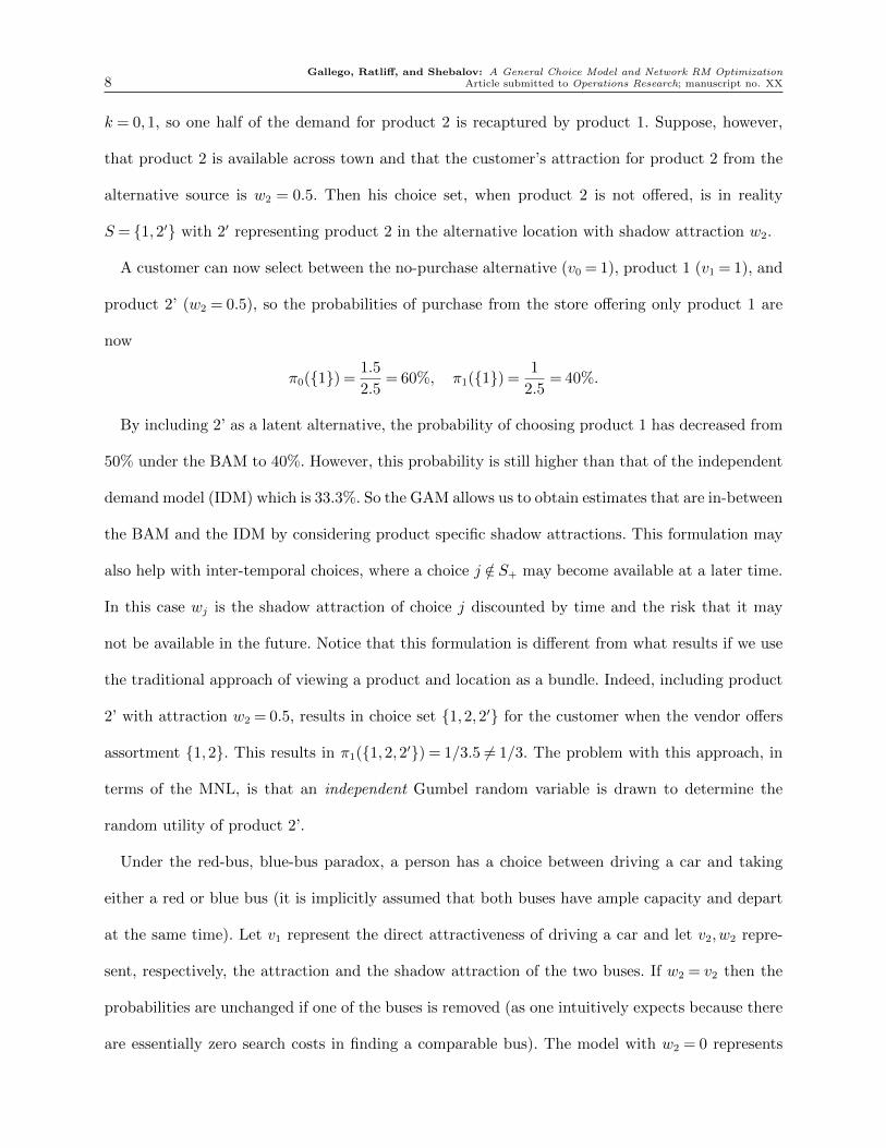
k = 0,1, so one half of the demand for product 2 is recaptured by product 1. Suppose, however,

that product 2 is available across town and that the customer’s attraction for product 2 from the

alternative source is w2 = 0.5. Then his choice set, when product 2 is not offered, is in reality

S = {1,2′} with 2′ representing product 2 in the alternative location with shadow attraction w2.

A customer can now select between the no-purchase alternative (v0 = 1), product 1 (v1 = 1), and

product 2’ (w2 = 0.5), so the probabilities of purchase from the store offering only product 1 are

now

π0({1}) =1.5

2.5= 60%, π1({1}) =

1

2.5= 40%.

By including 2’ as a latent alternative, the probability of choosing product 1 has decreased from

50% under the BAM to 40%. However, this probability is still higher than that of the independent

demand model (IDM) which is 33.3%. So the GAM allows us to obtain estimates that are in-between

the BAM and the IDM by considering product specific shadow attractions. This formulation may

also help with inter-temporal choices, where a choice j /∈ S+ may become available at a later time.

In this case wj is the shadow attraction of choice j discounted by time and the risk that it may

not be available in the future. Notice that this formulation is different from what results if we use

the traditional approach of viewing a product and location as a bundle. Indeed, including product

2’ with attraction w2 = 0.5, results in choice set {1,2,2′} for the customer when the vendor offers

assortment {1,2}. This results in π1({1,2,2′}) = 1/3.5 6= 1/3. The problem with this approach, in

terms of the MNL, is that an independent Gumbel random variable is drawn to determine the

random utility of product 2’.

Under the red-bus, blue-bus paradox, a person has a choice between driving a car and taking

either a red or blue bus (it is implicitly assumed that both buses have ample capacity and depart

at the same time). Let v1 represent the direct attractiveness of driving a car and let v2,w2 repre-

sent, respectively, the attraction and the shadow attraction of the two buses. If w2 = v2 then the

probabilities are unchanged if one of the buses is removed (as one intuitively expects because there

are essentially zero search costs in finding a comparable bus). The model with w2 = 0 represents


the case where there is no second bus. The common way to deal with the paradox is to use a nested

logit (NL) model. Under the NL model used to resolve the paradox, a person first selects a mode

of transportation and then one of the offerings within each mode. We are able to avoid the use of

the NL model, but as we shall see later, our model can be viewed as a limit of a NL model.

To formally define the GAM let S = {j ∈N : j /∈ S} be the complement of S in N = {1, . . . , n}.

In addition to the attraction values vj, there are shadow attraction values wj ∈ [0, vj], j ∈N such

that for any subset S ⊂N

πj(S) =vj

v0 +W (S) +V (S)j ∈ S, (2)

where for any R ⊂ N , W (R) =∑

j∈Rwj. Consequently, the no-purchase probability is given by

π0(S) = (v0 + W (S))/(v0 + W (S) + V (S)). In essence, the attraction value of the no-purchase

alternative has been modified to be v0 +W (S).

An alternative, perhaps simpler, way of presenting the GAM by using the following transforma-

tion: v0 = v0 +W (N) and vj = vj −wj, j ∈N . For S ⊂N , let V (S) =∑

j∈S vj. With this notation

the GAM becomes:

πj(S) =vj

v0 + V (S)∀j ∈ S and π0(S) = 1−πS(S). (3)

where πS(S) =∑

j∈S πj(S). Notice that all choice probabilities are non-negative as long as vj =

vj −wj ≥ 0 and v0 = v0 +∑

j∈N wj > 0, which holds when v0 > 0 and wj ∈ [0, vj] for all j ∈N .

The case wk = 0, k ∈N recovers the BAM, because v0 = v0 and vj = vj, j ∈N . In contrast, the

case wk = vk, k ∈N , results in v0 + V (S) = v0 + V (N) for all offered sets S ⊂N . The probability

πj(S), of selecting product j is independent of the set S containing j, resulting in the independent

demand model (IDM).

The parsimonious formulation P-GAM is given by wj = θvj ∀j ∈N for θ ∈ [0,1] can serve to

test H0 : θ= 0 vs H1 : θ > 0 to see whether the BAM applies or to test H0 : θ= 1 against H1 : θ < 1,

to see whether the IDM applies. If either of these tests fail, then a GAM maybe a better fit to the

data.


We provide two justifications for the GAM. The first justification is Axiomatic. The second

is a limiting case of the nested logit (NL) model. Readers who are not interested in the formal

derivation of the GAM can skip to section 2.4 for a method to estimate the GAM parameters.

2.1. Axiomatic Justification

Luce (1959) proposed two choice axioms. To describe the axioms under the assumption that the

no-purchase alternative is always available we will use the notation πS+(T ) =∑

j∈S+ πj(T ) for all

S ⊂ T and will use set difference notation T − S = T ∩ S to represent the elements of T that are

not in S. The Luce axioms are given by :

• Axiom 1: If πi({i})∈ (0,1) for all i∈ T , then for any R⊂ S+, S ⊂ T

πR(T ) = πR(S)πS+(T ).

• Axiom 2: If πi({i}) = 0 for some i∈ T , then for any S ⊂ T such that i∈ S

πS(T ) = πS−{i}(T −{i}).

The most celebrated consequence of the Luce Axioms, due to Luce (1959), is that πi(S) satisfies

the Luce Axioms if and only if there exist attraction values vj, j ∈N+ such that equation (1) holds.

Since its original publication, the paper Luce (1959) has been cited thousands of times. Among

the most famous citations, we find the already mentioned paper by McFadden (1974) that shows

that the only random utility model that is consistent with the BAM is the one with independent

Gumbel errors. An early paper by Debreu (1960), criticizes the Luce model as it suffers from the so

called independence of irrelevant alternatives (IIA). The IIA states the relative preference between

two alternatives does not change as additional alternatives are added to the choice set. Debreu,

however, suggests that the addition of an alternative to an offered set hurts alternatives that are

similar to the added alternative more than those that are dissimilar to it. To illustrate this, Debreu

provides an example that is a precursor to the red-bus, blue-bus paradox based on the choice

between three records: a suite by Debussy, and two different recordings of the same Beethoven


symphony. Another famous paper by Tversky (1972), criticizes both the Luce model as well as all

random utility models that assume independent utilities for their inability to deal with the IIA.

Tversky offers the elimination by aspects theory as a way to cope with the IIA. Others, such as n

Domenich and McFadden (1975) and Williams (1977), have turned to the nested logit (NL) model

as an alternative way of dealing with the IIA. Under a nested logit model, for example, a person

will first chose between modes of transportation (car or bus) before selecting a particular car or

bus color.

To our knowledge no one has altered the Luce Axioms with the explicit goal of modifying the

recapture probabilities. Yellott (1977), however, gives a characterization of the Luce model by an

axiom which he called invariance under uniform expansion of the choice set, which is weaker than

Luce’s Axiom but implies Luce’s Axiom when the choice model is assumed to be an independent

random utility model. The reader is also refereed to Dagsvik (1983), who expands Yellott’s ideas

to choices made over time.

Notice that Axiom 1 holds trivially for R= ∅ since π∅(S) = 0 for all S ⊂N . For ∅ 6=R⊂ S the

formula can be written as the ratio of the demand captured by R when we add T − S to S. The

ratio is given by

πR(T )

πR(S)= πS+(T ) = 1−πT−S(T ),

and is independent of R⊂ S. Our goal is to generalize Axiom 1 so that the ratio remains indepen-

dent of R⊂ S but in such a way that we have more control over the proportion of the demand that

goes to T −S. This suggests the following generalization of Axiom 1.

• Axiom 1’: If πi({i})∈ (0,1) for all i∈ T , then for any ∅ 6=R⊂ S ⊂ T

πR(T )

πR(S)= 1−

∑j∈T−S

(1− θj)πj(T )

for some set of values θj ∈ [0,1], j ∈N .

We will call the set of Axioms 1’ and 2 the Generalized Luce Axioms (GLA). We can think of

θj ∈ [0,1] as a relative measure of the competitiveness of product j in the market place. The next


result states that a choice model satisfies the GLA if and only if it is a GAM and links θj to the

ratio of wj to vj.

Theorem 1. A choice model πi(S) satisfies the GLA if and only if it is of the GAM form. More-

over, wj = θjvj for all j ∈N .

A proof of this theorem may be found in the Appendix. Notice that it is tempting to relax the

constraint wj ≥ 0 as long as v0 > 0. However, this relaxation would lead to a violation of Axiom 2.

2.2. GAM as Limit of Nested Logit Model under Competition

We now show that the GAM also arises as the limit of the nested logit (NL) model. The NL model

was originally proposed in Domenich and McFadden (1975), and later refined in McFadden (1978),

where it is shown that it belongs to the class of Generalized Extreme Value (GEV) family of models.

Under the nested choice model, customers first select a nest and then an offering within the nest.

The nests may correspond to product categories and the offerings within a nest may correspond

to different variants of the product category. As an example, the product categories may be the

different modes of transportation (car vs. bus) and the variants may be the different alternatives

for each mode of transportation (e.g., the blue and the red buses). As an alternative, a product

category may consist of a single product, and the variants may be different offerings of the same

product by different vendors. We are interested in the case where the random utility of the different

variants of a product category are highly correlated. The NL model, allows for correlations for

variants in nest i through the dissimilarity parameter γi. Indeed, if ρi is the correlation between

the random utilities of nest i offerings, then γi =√

1− ρi is the dissimilarity parameter for the nest.

The case γi = 1 corresponds to uncorrelated products, and to a BAM. The MNL is the special case

where the idiosyncratic part of the utilities are independent and identically distributed Gumbel

random variables.

Consider now a NL model where the nests correspond to individual products offered in the

market. Customers first select a product, and then one of the vendors offering the selected product.


Let Ok be the set of vendors offering product k, Sl be the set of products offered by vendor l, and

vkl be the attraction value of product k offered by vendor l. Under the NL model, the probability

that a customer selects product i∈ Sj is given by

πi(Sj) =

(∑l∈Oi

v1/γiil

)γiv0 +

∑k

(∑l∈Ok

v1/γkkl

)γk v1/γiij∑

l∈Oiv

1/γiil

, (4)

where the first term is the probability that product i is selected and the second term the probability

that vendor j is selected. Many authors, e.g., Greene (1984), use what is know as the non-normalized

nested models where vij’s are not raised to the power 1/γi. This is sometimes done for convenience

by simply redefining vkl← v1/γkkl . There is no danger in using this transformation as long as the γ’s

are fixed. However, the normalized model presented here is consistent with random utility models,

see Train (2002), and we use the explicit formulation because we will be taking limits as the γ’s

go to zero.

It is easy to see that πi(Sj) is a BAM for each vendor j, when γi = 1 for all i. This case can be

viewed as a random utility model, where an independent Gumbel random variable is associated with

each product and each vendor. Consider now the case where γi ↓ 0 for all i. At γi = 0, the random

utilities of the different offerings of product i are perfectly and positively correlated. This makes

sense when the products are identical and price and location are the only things differentiating

vendors. When these differences are captured by the deterministic part of the utility, then a single

Gumbel random variable is associated with each product. In the limit, customers select among

available products and then buy from the most attractive vendor. If several vendors offer the same

attraction value, then customers select randomly among such vendors. The next result shows that

a GAM arises for each vendor, as γi ↓ 0 for all i.

Theorem 2. The limit of (4) as γi ↓ 0 for all i is a GAM. More precisely, there are attraction

values akj, akj ∈ [0, akj], and a0j ≥ 0, such that the discrete choice model for vendor j is given by

πi(Sj) =aij

a0j +∑

k∈Sjakj

∀i∈ Sj.


This shows that if customers first select the product and then the vendor, then the NL choice

model becomes a GAM for each vendor as the dissimilarity parameters are driven down to zero.

The proof of this result is in the Appendix. Theorem 2 justifies using a GAM when some or all

of the products offered by a vendor are also offered by other vendors, and customers have a good

idea of the price and convenience of buying from different vendors. The model may also be a

reasonable approximation when products in a nest are close substitutes, e.g., when the correlations

are high but not equal to one. Although we have cast the justification as a model that arises from

external competition, the GAM also arises as the limit of a NL model where a firm has multiple

versions of products in a nest. At the limit, customers select the product with the highest attraction

within each nest. Removing the product with the highest attraction from a nest shifts part of the

demand to the product with the second highest attraction , and part to the no-purchase alternative.

Consequently a GAM of this form can be used in Revenue Management to model buy up behavior

when there are no fences, and customers either buy the lowest available fare for each product or

do not purchase.

2.3. Limitation and Heuristic Uses of the GAM

One limitation of the GAM as we propose it is that, in practice, the attraction and shadow attrac-

tion values may depend on a set of covariates that may be customer or product specific. This can be

dealt with either by assuming a latent class model on the population of customers or by assuming

a customer specific random set of coefficients to capture the impact of the covariates. This results

in a mixture of GAMs. The issues also arise when using the BAM. In practice, often a single BAM

is used to try to capture the choice probabilities of customers that may come from different market

segments. This stretches both models, as this should really be handled by adding market segments.

However the GAM can cope much better with this situation as the following example illustrates.

Example 1: Suppose there are two stores (denoted l), and each store attracts half of the

population. We will assume that there are two products (denoted k) and that the GAM parameters

vlk and wlk for the two stores are as given in Table 1:


v10 v11 v12 v20 v21 v22

w11 w12 w21 w22

1 1 1 1 0.9 0.90.9 0.8 0.8 0.7

Table 1 Attraction Values (v,w)

With this type of information we can use the GAM to compute choice probabilities πj(S) that

a customer will purchase product j ∈ S from Store 1 when Store 1 offers set S, and Store 2 offers

set R = {1,2}. Suppose Store 1 has observed selection probabilities for different offer sets S as

provided in Table 2:

S π0(S) π1(S) π2(S)∅ 100% 0% 0%{1} 82.1% 17.9% 0%{2} 82.8% 0.0% 17.2%{1,2} 66.7% 16.7% 16.7%

Table 2 Observed πj(S,R) for R= {1,2}

To estimate these choice probabilities using a single market GAM we found the values of

vk,wk, k= 1,2 with v0 = 1 that minimizes the sum of squared errors of the predicted probabilities.

This results in the GAM model: v0 = 1, v1 = v2 = 0.25, w1 = 0.20 and w2 = 0.15. This model per-

fectly recovers the probabilities in Table 2. However, when limited to the BAM, the largest error

is 1.97% in estimating π0({1,2}).

This improved ability to fit the data comes at a cost because the GAM requires estimating w in

addition to v. As we will see in the next section, it is possible to estimate the v and w from the

store’s offer sets and sales data. We will assume, as in any estimation of discrete choice modeling,

that the same choice model prevails over the collected data set. If this is not the case, then the

estimation should be done over a subset of the data where this assumption holds. As such, we do

not require information about what the competitors are offering, only that their offer sets do not

vary over the data set. This is an implicit assumption made when estimating any discrete choice

model. The output of the estimation provides the store manager an indication of which products

face more competition by looking at the resulting estimates of the ratios θi = wi/vi. Over time,


a firm can estimate parametric or full GAM models that take into account what competitors are

offering and then update their choice models dynamically depending on what the competition is

doing.

2.4. GAM Estimation and Examples

It is possible to estimate the parameters of the GAM by refining and extending the Expectation

Maximization method developed by VvRR (Vulcano et al. (2012)) for the BAM. Readers not

interested in estimation can skip to Section 3. We assume that demands in periods t= 1, . . . , T arise

from a GAM with parameters v and w and arrival rates λt = λ for t= 1, . . . , T . The homogeneity

of the arrival rates is not crucial. In fact the method described here can be extended to the case

where the arrival rates are governed by co-variates such as the day of the week, seasonality index,

and indicator variables of demand drivers such as conferences, concerts or other events that can

influence demand. Our main purpose here is show that it is possible to estimate demands fairly

accurately. The data are given by the offer sets St ⊂N and the realized sales zt ⊂Zn+, excluding the

unobserved value of the customers who chose the no-purchase alternative, for t= 1, . . . , T . VvRR

assume that the market share s= πN(N), when all products are offered, is known. While we do

not make this assumption here, we do present results with and without knowledge of s.

VvRR update estimates of v by estimating demands for each of the products in N when some of

them are not offered. To see how this is done, consider a generic period with offer set S ⊂N,S 6=N

and realized sales vector Z = z. Let Xj be the demand for product j if set N instead of S was

offered. We will estimate Xj conditioned on Z = z. Consider first the case j /∈ S. Since Xj is

Poisson with parameter λπj(N), substituting the MLE estimate λ= e′z/πS(S) of λ we obtain the

estimate Xj = λπj(N) =πj(N)

πS(S)e′z. We could use a similar estimate for products j ∈ S but this would

disregard the information zj. For example, if zj = 0 then we know that the realization of Xj was

zero as customers had product j available for sale. We can think of Xj, conditioned on (S, z) as a

binomial random variable with parameters zj and probability of selection πj(N)/πj(S). In other

words, each of the zj customers that selected j when S was available, would have selected j anyway


with probability πj(N)/πj(S). Then Xj =πj(N)

πj(S)zj is just the expectation of the binomial. Notice

that X[1, n] =∑m

i=1 Xj = e′zπS(S)

πN(N) = λs. We can find X0 by treating it as j /∈ S resulting in

X0 = π0(N)

πS(S)e′z = λ(1− s). We summarize the results in the following proposition:

Proposition 1. (VvRR extended to the GAM): If j ∈ S then

Xj =πj(N)

πj(S)zj.

If j /∈ S or j = 0 we have

Xj =πj(N)

πS(S)e′z.

Moreover, X[1, n] =∑

j∈N Xj = πN (N)

πS(S)e′z.

VvRR use the formulas for the BAM to estimate the parameters λ, v1, . . . , vn under the assump-

tion that the share s= v(N)/(1 + v(N)) is known. From this they use an E-M method to iterate

between estimating the Xjs given a vector v and then optimizing the likelihood function over v

given the observations. The MLE has a closed form solution so the updates are given by vj = Xj/X0

for all j ∈N , where X0 = rX[1, n] and r = 1/s− 1. VvRR use results in Wu (1983) to show that

the method converges. We now propose a refinement of the VvRR method that can significantly

reduce the estimation errors.

Using data (St, zt), t = 1 . . . , T , VvRR obtain estimates Xtj that are then averaged over the T

observations for each j. In effect, this amounts to pooling estimators from the different sets by

giving each period the same weight. When pooling estimators it is convenient to take into account

the variance of the estimators and give more weight to sets with smaller variance. Indeed, if we

have T different unbiased estimators of the same unknown parameter, each with variance σ2t , then

giving weights proportional to the inverse of the variance minimizes the variance of the pooled

estimator. Notice that the variance of Xtj is proportional to 1/πj(St) if j ∈ St and proportional to

1/πSt(St) otherwise. Let atj = πj(St) if j ∈ St and atj = πSt(St) if j /∈ St. We can select the set the

weights for product j as

ωtj =atj∑T

s=1 asj.


Our numerical experiments suggests that using this weighting scheme reduces the variance of the

estimators by about 4%.

To extend the procedure to the GAM we combine ideas of the EM method based on MLEs and

least squares (LS). It is also possible to refine the estimates by using iterative re-weighted least

squares (Green (1984) and Rubin (1983)) but our computational experience shows that there is

little benefit from doing this. To initialize the estimation we use formulas for the expected sales

under St, t= 1, . . . , T for arbitrary parameters λ, v and w. More precisely, we estimate E[Ztj] by

λπj(St) = λvj

v0 +V (S) +W (S)j ∈ St, t∈ {1, . . . , T}.

We then minimize the sum of squared errors between estimated and observed sales (zts):

T∑t=1

∑i∈St

[λ

vjv0 +V (S) +W (S)

− zti]2

,

subject to the constraints 0 ≤ w ≤ v and λ ≥ 0. This is equivalent to maximizing the likelihood

function ignoring the unobserved values of the no-purchase alternative zt0.

This gives us an initial estimate λ(0), v(0),w(0) and an initial estimate of the market share s(0) =

v(0)(N)/(1 + v(0)(N)). Let r(0) = 1/s(0) − 1. If s is known then we add the constraint v(N) = r =

1/s− 1. Given estimates of v(k) and w(k) the procedure works as follows:

E-step: Estimate the first choice demands X(k)tj and then aggregate over time using the current

estimate of the weights α(k)tj to produce X

(k)j =

∑T

t=1 X(k)tj α

(k)tj and X

(k)0 = r(k)X(k)[1, n] and update

the estimates of v by

v(k+1)j =

X(k)j

X(k)0

j ∈N.

M-step: Feed v(k+1) together with arbitrary λ and w to estimate sales under St, t= 1, . . . , T and

minimize the sum of squared errors between observed and expected sales over λ and w subject to

w≤ v(k+1) and non-negativity constraint to obtain updates λ(k+1), w(k+1) and s(k+1).

The proof of convergence is a combination of the arguments in Wu, as in VvRR, and the fact

that the least squared errors problem is a convex minimization problem. The case when s is known


works exactly as above, except that we do not need to update this parameter. The M-step can be

done by solving the score equations:

∑t∈Ai

πi(St)[e′zt +λπ0(St)]−

∑t∈Ai

zti = 0 i= 1, . . . , n,

∑t/∈Ai

πi(St)[e′zt +λπ0(St)]−λ

∑t/∈Ai

πi(St) = 0 i= 1, . . . , n.

andT∑t=1

πSt(St)−T∑t=1

e′zt/λ= 0,

where Ai is the set of periods where product i is offered and

πi(St) =vi

1 +V (St) +W (St)t /∈Ai.

This is a system of up to 2n+ 1 equations on 2n+ 1 unknowns. Attempting to solve the score

equations directly or through re-weighted least squares does not materially improve the estimates

relative to the least square procedure described above.

We now present three examples to illustrate how the procedure works in three different cases:

1) w= 0 corresponding to the BAM, 2) w= θv corresponding to the (parsimonious) p-GAM, and

3) 0 6=w ≤ v corresponding to the GAM. These examples are based on Example 1 in VvRR. The

examples involve five products and 15 periods where the set N = {1,2,3,4,5} was offered in four

periods, set {2,3,4,5} was offered in two periods, while sets {3,4,5},{4,5} and {5} were each

offered in three periods. Notice that product 5 is always offered making it impossible to estimate

w5. On the other hand, estimates of w5 would not be needed unless the firm planned to not offer

product 5.

In their paper, VvRR present the estimation results for a specific realization of sales zt, t =

1, . . . , T = 15 corresponding to the 15 offer sets St, t= 1, . . . ,15. We instead generate 500 simulated

instances of sales, each over 15 periods, and then compute our estimates for each of the 500

simulations. We report the mean and standard deviation of λ, v and either θ or w over the 500


simulations. We feel these summary statistics are more indicative of the ability of the method

to estimate the parameters. We report results when s (historical market share) is assumed to be

known, as in Vulcano et al. (2012), and some results for the case when s is unknown (see 1. in the

endnotes).

Estimates of the model parameters tend to be quite accurate when s is known and the estimation

of λ and v become more accurate when w 6= 0. The results for s unknown tend to be accurate when

w= 0 but severely biased when w 6= 0. The bias is positive for v and w and negative for λ. Since it is

possible to have biased estimates of the parameters but accurate estimates of demands, we measure

how close the estimated demands λπi(S) = λ vi1+v(S)+w(S)

i∈ S, S ⊂N are from the true expected

demands λπi(S), i∈ S, S ⊂N and also how close the estimated demands λπi(St) i∈ St, t= 1, . . . , T

are from sales zti, i∈ St, t= 1, . . . , T . These measures are reported, respectively, as the Model Mean

Squared Error (M-MSE ) and the traditional Mean Squared Error (MSE) between the estimates

and the data. Surprisingly the results with unknown s, although strongly biased in terms of the

model parameters, often produce M-MSEs and MSEs that are similar to the corresponding values

when s is known.

Example 2 (BAM) In the original VvRR example, the true value of w is 0. The estimates with

s known and s unknown as well as the true values of the parameters are given in Table 3.

s λ v1 v2 v3 v4 v5

known 50.27 0.988 0.700 0400 0.200 0.050unknown 51.26 1.212 0.818 0.449 0.219 0.053true 50.00 1.000 0.700 0.400 0.200 0.050

Table 3 Estimated values of λ and v with s known

The MSE and the M-MSE were respectively 247.50 and 58.44, for both the case of s known and

unknown.

Example 3 (P-GAM) For this example v is the same as above but w = θv with θ = 0.20. The

results are given in Table 4. Notice that the estimate of θ is more accurate for the case of s unknown.

Clearly the estimated values with s known are much closer to the actual values. However, the fit

to the model and to data for the case of s unknown is similar to the case of s known. Indeed, the


s λ v1 v2 v3 v4 v5 θknown 50.12 0.988 0.702 0.397 0.201 0.051 0.238unknown 4.390 0.111 0.079 0.062 0.035 0.014 0.219true 50.00 1.000 0.700 0.400 0.200 0.050 0.200

Table 4 Estimated values of λ, v and θ with s known

MSE and the M-MSE were respectively 226.2 and 50.37 for the case of s known and 228.54 and

53.84, respectively, for the case of s unknown. This suggests that the parameter values that can be

far from the true parameters and yet have a sufficiently close fit to the model and to the data.

Example 4 (GAM) For this example λ and v are as above, and w= (0.25,0.35,0.15,0.05,0.05).

The results are given in Table 5.

s λ v1 v2 v3 v4 v5 w1 w2 w3 w4 w5

known 50.19 0.994 0.700 0.404 0.202 0.051 0.321 0.288 0.186 0.106 0.010true 50.00 1.000 0.700 0.400 0.200 0.050 0.250 0.350 0.150 0.050 0.050

Table 5 Estimated values of λ, v and w with s known and unknown

Notice that the estimated values of λ and v for the case of v known are better under the GAM

than for the case w= 0 or w= θv. The MSE and M-MSE are respectively 204.71 and 48.56 for the

case of s known. The estimates of the parameters are severely biased when s is unknown so are not

reported. However, the MSE and M-MSE were respectively, 203.70 and 54.33, a surprisingly good

fit to data. This again suggests that there is a ridge of parameter values that fit the data and the

model well.

3. Stochastic Revenue Management over a Network

In this section we present the formulation for the stochastic revenue management over a network.

We will assume that there are L customer market segments and that customers in a particular

market segment are interested in a specific set of itineraries and fares (see 2. in the endnotes) from

a set of origins to one or more destinations. For example, a market segment could be morning

flights from New York to San Francisco that are less than $500, or all flights from New York

City to the Mexican Caribbean. Notice that there may be multiple fares with different restrictions

associated with each itinerary. At any time the set of origin-destination-fares (ODFs) offered for


sale to market segment l is a subset Sl ⊂Nl, l ∈L= {1, . . . ,L} where Nl is the consideration set for

market segment l ∈L with associated fares plk, for each product k in nest Nl. If the consideration

sets are non-overlapping over the market segments then there is no need to add further restrictions

to the offered sets. This is also true when consideration sets overlap if the capacity provider is free

to independently decide what fares to offer in each market. As an example, round-trips from the

US to Asia are sold both in Asia and the US. If the carrier can charge different fares depending

on whether the customer buys the fare in the US or in Asia, then no further restrictions are

needed. Otherwise, he needs to impose restrictions so that the same set of products is offered in

both markets. One way to handle this is to post a single offer set S at a time, so then use the

projection subsets Sl = S ∩Nl for all markets l that are constrained to offers the same price for

offered fares. Customers in market segment l select from Sl and the no-purchase alternative. We

will abuse notation slightly and write πlk(Sl) to denote the probability of selecting product k ∈ Sl+

from market segment l. For convenience we define πlk(Sl) = 0 if k /∈ Sl+.

The state of the system will be denoted by (t, x) where t is the time-to-go and x is an m-

dimensional vector representing remaining inventories. The initial state is (T, c) where T is the

length of the horizon and c is the initial inventory capacity. For ease of exposition we will assume

that customers arrive to market segment l as a Poisson process with time homogeneous rate λl.

We will denote by J(t, x) the maximum expected revenues that can be obtained from state (t, x).

The Hamilton-Jacobi-Bellman (HJB) equation is given by

∂J(t, x)

∂t=∑l∈L

λl maxSl⊂Nl

∑k∈Sl

πlk(Sl) (plk−∆lkJ(t, x)) (5)

where ∆lkJ(t, x) = J(t, x)− J(t, x−Alk), where Alk is the vector of resources consumed by k ∈Nl

(e.g. flight legs on a connecting itinerary class). The boundary conditions are J(0, x) = 0 and

J(t,0) = 0. Talluri and van Ryzin (2004) developed the first stochastic, choice-based, dependent

demand model for the single resource case in discrete time. The first choice-based, network

formulation is due to Gallego et al. (2004).


4. The Choice Based Linear Program

An upper bound J(T, c) on the value function J(T, c) can be obtained by solving a deterministic

linear program. The justification for the bound can be obtained by using approximate dynamic

programming with affine functions.

We now introduce additional notation to write the linear program with value function J(T, c)≥

J(T, c). Let πl(Sl) be the nl = |Nl|-dimensional vector with components πlk(Sl), k ∈ Nl. Clearly

πl(Sl) has zeros for all k /∈ Sl. The vector πl(Sl) gives us the probability of sale for each fare in Nl

per customer when we offer set Sl. Let rl(Sl) = p′lπl(Sl) =∑

k∈Nlplkπlk(Sl) be the revenue rate per

customer associated with offering set Sl ⊂Nl where pl = (plk)k∈Nlis the fare vector for segment

l ∈L. Notice that πl(∅) = 0∈<nl and rl(∅) = 0∈<. Let Alπl(Sl) be the consumption rate associated

with offering set Sl ⊂Nl where Al is a matrix with columns Alj associated with ODF j ∈Nl.

The choice based deterministic linear program (CBLP) for this model can be written as

J(T, c) = max∑

l∈L λlT∑

Sl⊂Nlrl(Sl)αl(Sl)

subject to∑

l∈L λlT∑

Sl⊂NlAlπl(Sl)αl(Sl) ≤ c∑

Sl⊂Nlαl(Sl) = 1 l ∈L

αl(Sl) ≥ 0 Sl ⊂Nl l ∈L.

(6)

The decision variables are αl(Sl), Sl ⊂ Nl, l ∈ L which represent the proportion of time that set

Sl ⊂Nl is used. The case of non-homogeneous arrival rates can be handled by replacing λlT by∫ T0λlsds. There are

∑l∈L 2nl decision variables. Gallego et al. (2004) showed that J(T, c)≤ J(T, c)

and proposed an efficient column generation algorithm for a class of attraction models that

includes the BAM. This formulation has been used and analyzed by other researchers including

Bront et al. (2009), Kunnumkal and Topaloglu (2010), Kunnumkal and Topaloglu (2008), Liu and

van Ryzin (2008) and Zhang and Adelman (2009).

5. The Sales Based Linear Program for the GAM

In this section we will present a linear program that is equivalent to the CBLP for the GAM, but

is much smaller in size (essentially the same size as the well known IDM) and easier to solve (as


it avoids the need for column generation). The new formulation is called the sales based linear

program (SBLP) because the decision variables are sales quantities. The number of variables in

the formulation is∑

l∈L(nl + 1), where xlk, k= 0,1 . . . , nl, l ∈L represents the sales of product k in

market segment l. Let the aggregate market demand for segment l be denoted by Λl = λlT, l ∈ L

(or∫ T

0λlsds if the arrival rates are time varying) inclusive of the no-purchase alternative. With

this notation the formulation of the SBLP is given by:

R(T,c)= max∑

l∈L∑

k∈Nlplkxlk

subject to

capacity :∑

l∈L∑

k∈NlAlkxlk ≤ c

balance : vl0vl0xl0 +

∑k∈Nl

vlkvlkxlk = Λl l ∈L

scale : xlkvlk− xl0

vl0≤ 0 k ∈Nl l ∈L

non-negativity: xlk ≥ 0 k ∈Nl l ∈L

(7)

Theorem 3. If each market segment πlj(Sl) is of the GAM form (2) then J(T, c) =R(T, c).

We demonstrate the equivalence of the CBLP and SBLP formulations by showing that the SBLP

is a relaxation of the CBLP and then proving that the dual of the SBLP is a relaxation of the dual

of the CBLP. Full details of this proof may be found in the Appendix.

The intuition behind the SBLP formulation is as follows. Our decision variables represent the

amount of inventory to allocate for sales across ODFs for different market segments. The objective

is to maximize revenues. Three types of constraints are required. The capacity constraints limit

the sum of the allocations. The balance constraints ensure that the sale allocations are in certain

hyperplanes, so when some service classes are closed for sale, the demands for the remaining open

service classes (including the null alternative) changes dependently; they must be modified to offset

the amount of the closed demands. The scale constraints operate on the principle that demands

are rescaled depending on both the availability and the attractiveness of other items in the choice

set.

The decision variables xl0 play an important role in the SBLP. Since the null alternative has

positive attractiveness and is always available, the dependent demand for any service class is


upper bounded based on its size relative to the null alternative. The scale constraints imply that

xlk/vlk ≤ xl0/vl0. Therefore, the scale constraints favor a large value of xl0. On the other hand,

the balance constraint can be written as∑

k∈N vlkxlk/vlk ≤ Λl − vl0xl0/vl0, favoring a small value

of xl0. The LP solves for this tradeoff taking into account the objective function and the capacity

constraint. We will have more to say about xl0 in the absence of capacity constraints in Section 6.

The combination of the balance and scale constraints ensures that GAM properties are compactly

represented in the optimizer and that the correct ratios are maintained between the sizes of each

of the open alternatives.

For the BAM the demand balance constraint simplifies to xl0 +∑

k∈Nlxlk = Λl. For the inde-

pendent demand case, vl0 = vl0 +∑

k∈Nlvlk and vlk = 0 for k ∈Nl. The balance constraint reduces

to xl0 = (vl0/vl0)Λl, and the scale constraint becomes xlk ≤ (vlk/vl0)Λl, k ∈ Nl, so clearly xl0 +∑k∈Nl

xlk ≤Λl.

We remark that the CBLP and therefore the SBLP can be extended to multi-stage problems

since the inventory dynamics are linear. This allows for different choice models of the GAM family

to be used in different periods and is the typical approach in practice.

5.1. Recovering the Solution for the CBLP

So we have learned that the SBLP problem is much easier to solve and provides the same revenue

performance as the CBLP. However, there are some circumstances (described later in this section)

in which it is more desirable to use the CBLP solution. The reader may wonder whether it is

possible to recover the solution to the CBLP from the solution to the SBLP. In other words, is it

possible to obtain a collection of offer sets {S : α(S)> 0} that solves the CBLP from the solution

xlk, k ∈ Nl, l ∈ L of the SBLP? The answer is yes, and the method presented here for the GAM

is inspired by Topaloglu et al. (2011) who used our SBLP formulation and presented a method

to recover the solution to the CBLP for the BAM. When used with the GAM, recovering the

CBLP solution is important because solutions in terms of assortments tend to be more robust then

solutions in terms of sales. Indeed, our experience is that when GAM parameters are estimated,


the solution in terms of sales can be fairly far from the solution with known parameters, whereas

the solution in terms of assortments tends to be much closer.

In this section we will show how to obtain the solution of the CBLP from the SBLP and will also

show that for each market segment the offered sets are nested in the sense that there exist subsets

Slk increasing in k with positive weights. The products in the smallest set are core products that

are always offered. Larger sets contain additional products that are only offered part of the time.

The sorting of the products is not by revenues, but by the ratio of xlk/vlk for all k ∈Nl ∪ {0} for

each l ∈ L. We then form the sets Sl0 = ∅ and Slk = {1, . . . , k} for k = 1, . . . , nl, where nl = |Nl| is

the cardinality of Nl. For k= 0,1, . . . , nl, let

αl(Slk) =

(xlkvlk− xl,k+1

vl,k+1

)V (Slk)

Λl

,

where for convenience we define xl,nl+1/vl,nl+1 = 0. Set αl(Sl) = 0 for all Sl ⊂ Nl not in the col-

lection Sl0, Sl1, . . . , Slnl . It is then easy to verify that αl(Sl)≥ 0, that∑

Sl⊂Nlαl(Sl) = 1, and that∑

Sl⊂Nlαl(Sl)πlk(Sl) = xlk. Applying this to the CBLP we can immediately see that all constraints

are satisfied, and the objective function coincides with that of the SBLP. Notice that for each

market segment the offered sets are nested Sl0 ⊂ Sl1 ⊂ . . .⊂ Slnl , and that set Slk is offered for a

positive fraction of time if and only if xlk/vlk > xl,k+1/vl,k+1. Unlike the BAM and the IDM, the

sorting order of products under the GAM is not necessarily revenue ordered. This is because fares

that face more competition (wlj close to vlj) are more likely to be offered even if their corresponding

fares are low.

5.2. Bounds and Numerical Examples

In this section we present two results that relate the solutions to the extreme cases w= 0 and w= v

to the case 0≤w≤ v. The proofs of the propositions are in the Appendix.

The reader may wonder whether the solution that assumes wj = 0 for all j ∈N is feasible when

wj ∈ (0, vj) j ∈N . The following proposition confirms and generalizes this idea.


Proposition 2. Suppose that αl(Sl), Sl ⊂ Nl, l ∈ L is a solution to the CBLP for the GAM for

fixed vlk, k ∈Nl+, l ∈ L and wlk ∈ [0, vlk], k ∈Nl, l ∈ L. Then αl(Sl), Sl ⊂Nl, l ∈ L is a feasible, but

suboptimal, solution for all GAM models with w′lk ∈ (wlk, vlk], k ∈Nl, l ∈L.

An easy consequence of this proposition is that if αl(Sl), l ∈ L is an optimal solution for the

CBLP under the BAM, then it is also a feasible, but suboptimal, solution for all GAMs with

wk ∈ (0, vk]. This implies that the solution to the BAM is a lower bound on the revenue for the

GAM with wk ∈ (0, vk] for all k.

As mentioned in the introduction, the IDM underestimates demand recapture. As such optimal

solutions for the SBLP under the IDM are feasible but suboptimal solutions for the GAM. The

following proposition generalizes this notion.

Proposition 3. Suppose that xlk, k ∈Nl, l ∈ L is an optimal solution to the SBLP for the GAM

for fixed vlk, k ∈Nl+ and wlk ∈ [0, vlk], k ∈Nl, l ∈L. Then xlk, k ∈Nl+, l ∈L is a feasible solution for

all GAM models with w′lk ∈ [0,wlk], k ∈Nl, l ∈L with the same objective function value.

An immediate corollary is that if xlk, k ∈Nl, l ∈ L is an optimal solution to the SBLP under the

independent demand model then it is also a feasible solution for the GAM with wk ∈ [0, vk] with

the same revenue as the IDM. This implies that the solution to the IDM is another lower bound

on the GAM with wk ∈ [0, vk] for all k.

Example 5: The following example problem was originally reported in Liu and van Ryzin (2008).

There are three flights AB,BC and AC. All customers depart from A with destinations to either

B or C. The relevant itineraries are therefore AB,ABC and AC. For each of these itineraries

there are two fares (high and low) and three market segments. Market segment 1 are customers

who travel to B. Market segment 2 are customers who travel to C but only at a high fare. Market

segment 3 are customers who travel to C but only at the low fare. The six fares as well as vlj, j ∈Nl

and vl0 for l= 1,2,3 are given in Table 6. The arrivals are uniformly distributed over a horizon of

T = 15, and the expected market sizes are Λ1 = 6,Λ2 = 9,Λ3 = 15 and that capacity c= (10,5,5)

for flights AB, BC and AC.


1 2 3 4 5 6 0Products ACH ABCH ABH ACL ABCL ABL Null

Fares $1,200 $800 $600 $800 $500 $300(AB,v1j) 5 8 2

(AChigh, v2j) 10 5 5(AClow, v3j) 5 10 10

Table 6 Market Segment and Attraction Values v

In this example we will consider the parsimonious p-GAM model wlj = θvlj for all j ∈ Nl, l ∈

{1,2,3} for values of θ ∈ [0,1]. We will assume that the vlj values are known for all j ∈ Nl, l ∈

{1,2,3}, but the BAM and the IDM use the extreme values θ= 0 and θ= 1, while the GAM uses

the correct value of θ. This situation may arise if the model is calibrated based on sales when all

products are offered, e.g., Sl =Nl for all l ∈ {1,2,3}. The objective here is to study the robustness

of using the BAM and the IDM to the p-GAM for values of θ ∈ (0,1). The situation where the

parameters are calibrated from data that includes recapture will be presented in the next example.

The solution to the CBLP for the BAM is given by α({1,2,3}) = 60%, α({1,2,3,5}) = 23.3% and

α({1,2,3,4,5}) = 16.7% with α(S) = 0 for all other subsets of products. Equivalently, the solution

spends 18, 7 and 5 units of time, respectively, offering sets {1,2,3}, {1,2,3,5} and {1,2,3,4,5}. The

solution results in $11,546.43 in revenues (see 3. in the endnotes). By Proposition 2, the solution

α({1,2,3}) = 60%, α({1,2,3,5}) = 23.3%, α({1,2,3,4,5}) = 16.7% is feasible for all θ ∈ (0,1] with a

lower objective function value. The corresponding SBLP solution is shown in Table 7 and provides

the same revenue outcome as the CBLP.

1 2 3 4 5 6 0Products ACH ABCH ABH ACL ABCL ABL xl0 Profit(AB,x1j) 4.29 1.71 $2,571.43

(AChigh, x2j) 4.50 2.25 2.25 $7,200.00(AClow, x3j) 0.50 2.75 11.75 $1,775.00

Total 4.50 2.25 4.29 0.50 2.75 0.0 15.71 $11,546.43Table 7 SBLP Allocation Solution for BAM with (θ= 0)

The case θ = 1 corresponds to the IDM. The solution to the SBLP for the IDM and the cor-

responding revenue is given in Table 8. By Proposition 3, the solution to the IDM is a feasible

solution for all θ ∈ [0,1) with the same objective value function.


1 2 3 4 5 6 0Products ACH ABCH ABH ACL ABCL ABL xl0 Profit(AB,x1j) 2.00 3.00 0.80 $2,100.00


Total 4.50 2.25 2.00 0.50 2.75 3.00 9.05 $11,075.00Table 8 SBLP Allocation Solution for IDM with (θ= 1)

Rev

enue

$10,100

$10,200

$10,300

$10,400

$10,500

$10,600

$10,700

$10,800

$10,900

$11,000

$11,100

$11,200

$11,300

$11,400

$11,500

$11,600

Theta

0% 10% 20% 30% 40% 50% 60% 70% 80% 90% 100%

Legend

gam bam idm

Figure 1 GAM, BAM and IDM Revenue for Known θ ∈ [0,1] Values

Figure 1 shows how the two extreme solutions (CBLP for θ= 0) and (SBLP for θ= 1) perform

for the attraction values given in Table 6 when the true model is GAM with θ ∈ (0,1). Notice that

the BAM solution does well only for small values of θ, say θ≤ 20% and performs poorly for large

values of θ. Indeed, the BAM solution gives up about 10% of the optimal profits at the extreme

value of θ = 1. The case θ = 1 corresponds to the independent demand model, and in this case

the BAM anticipates demand recapture when there is none. A related finding was reported by

Hartmans (2006) of Scandinavian Airlines; his simulation studies showed clear positive revenue

potential of including recapture effects, but assuming strong recapture in cases where it does note

exist can lead to revenue losses. The solution for the IDM gives up significant profits only for small

values of θ. In particular, the IDM solution loses over 4% of the optimal profits for θ= 0 but less


than 0.25% of profits for θ≥ 40%.

The optimal value function for the GAM is only marginally better than the maximum of the

value functions for the BAM and the IDM. Notice that these results apply to the special case of the

p-GAM, where all products in the choice set have had their shadow attractions downgraded by the

same relative amount. In a more typical application, only products that face competition will have

positive shadow attractions, so we expect the revenue differences between the BAM and GAM not

to be as large as in Example 5. Nonetheless, the example does highlight the asymmetry of revenue

performance associated with overestimating versus underestimating recapture probabilities.

Example 6: One may wonder how the three models would compare, if the attraction values in

Example 5 were estimated from data. Estimating the parameters would give the BAM and the

IDM more flexibility to compensate for using the wrong value of θ. On the other hand, the burden

of estimating a p-GAM as either a BAM or an IDM, can put stress on the estimated parameter.

It is not clear, therefore, whether the gaps suggested by Figure 1 are indicative of the difference

in performance when the parameters need to be estimated. On the other hand, the GAM has one

more parameter to estimate. What is important, therefore is to ascertain whether the GAM can

result in significant improvements over the BAM and IDM, and whether the gaps are smaller or

larger than those in the figure.

We tested this for three values of θ: 0.1, 0.5 and 0.9. Based on Figure 1, at θ= 0.1, we expect the

BAM to do very well and the IDM to do poorly. At θ = 0.5, we expect the BAM to struggle and

the IDM to do well. Finally, at θ= 0.9 we expect the BAM to do poorly and the IDM to very well.

To evaluate the performance of the three models, we generated data, estimated the parameters,

solved the SBLP with the estimated parameters for each of the three models, and then evaluated,

via simulation, the performance of the heuristic that uses the offer sets recommended by the SBLP.

We then compute the relative performance of the BAM and the IDM to the GAM. We report the

average of the relative performance over 500 repetitions of the entire procedure.

We simulate 50 instances of demands for each of the three non-trivial subsets for each market

to generate the data to estimate the parameters. For example, market 1 consists of product 3 and


4, with non-trivial subsets {3},{4} and {3,4}. To estimate the parameters we used the procedure

described in Section 2.4. To solve the linear program, we used the SBLP and converted the solution

to the CBLP as indicated in Section 5.1. To evaluate the performance of the heuristic we simulated

1000 repetitions using the offer sets recommended by the heuristic. The implementation of the

heuristic always starts by offering the largest set within a market. All the simulated requests are

accepted on a first-come first-serve basis within capacity limits.

For θ= 0.1, all of the three models do a reasonably good job of estimating the attraction values.

All of the three models, agreed on offering product 3 all of the time. The GAM and the BAM

agreed on offering products 1 and 2 all of the time. The IDM model, however, would some times

offer product 2 by itself for short periods of time. For market 3, the BAM and the GAM, were

remarkably consistent on offering product 5 by itself about 28% of the time and products 4 and

5 about 14% of the time. We were surprised by this, given the often significant differences in

the estimated parameters. The IDM disagreed offered product 5 by itself about 28% of the time,

but rarely offered product 4 at all. The performance of the BAM was essentially identical to the

performance of the GAM, achieving close to 100% of the revenues obtained by the GAM heuristic.

The IDM model, on the other hand, yielded about 98.2% of the revenue of the GAM heuristic.

For θ= 0.5, the estimates of the parameters for both the GAM and the IDM are fairly close to

the actual values. This is not so for the BAM, that makes a huge effort to accommodate for the

partial recapture resulting from θ= 0.5. Table 9 illustrates the true parameters and the estimated

values for the BAM, GAM, and IDM for one instance of the problem. Remarkably, even though

the estimates of the parameters for the BAM are often way off, the recommendations made by the

BAM were not far from those made by the GAM when viewed as solutions of the CBLP. In fact,

for the estimated values in Table 9, the recommendations were nearly identical: Offer products 1,2

and 3 all the time. Offer product 4 and 5 together 16% of the time, and offer product 5 by itself

27% of the time. The IDM solution for the reported instance in Table 9 was consistent with the

BAM and GAM for markets segments 1 and 2, but offered products 4 and 5 together 4% of the

time, and product 5 by itself 34% of the time.


Averaging over the 500 instances, the IDM was able to capture 99.45% of the revenues of the

GAM, while the BAM was able to capture 99.58%. This is contrast to Figure 1. These experiments

suggest that estimation helps the BAM relative to having the correct values of the attraction values

and the wrong value of θ, but it does not help the IDM as much.

v13 v16 v10 Λ1 θ v21 v22 v20 Λ2 θ v34 v35 v30 Λ3 θTrue 5.00 8.00 2.00 6.00 0.50 10.00 5.00 5.00 9.00 0.50 5.00 10.00 10.00 15.00 0.50BAM 3.79 8.38 1.87 5.00 0.00 5.19 2.35 12.46 17.54 0.00 3.05 6.77 15.18 23.17 0.00GAM 4.96 8.08 1.95 5.53 0.39 10.36 4.70 4.94 8.78 0.50 4.74 10.51 10.17 15.17 0.35IDM 5.34 7.85 1.81 6.40 1.00 10.06 5.04 4.89 9.64 1.00 5.00 9.99 10.00 16.78 1.00

Table 9 Estimates of Parameters when θ= 0.50

For θ= 0.9, the estimates of the parameters are way off for the BAM, while the estimates for the

GAM and the IDM are quite close to the actual values. Nevertheless, the three models continue

to agree in terms of offering products 1, 2 and 3 all the time for most instances of the problem.

For a particular instance, generated with the same seed as Table 9, the BAM, offers products 4

and 5 together 16% of the time and offers product 5 by itself 10% of the time. The IDM, offers

products 4 and 5 together 14% of the time and product 5 by itself 30% of the time. The GAM

offers products 4 and 5 together 16% of the time and product 5 by itself 27% of the time. Notice

that the GAM and the IDM solutions are very similar. But the BAM suffers because very little

demand is recaptured from product 6 and from product 4 when only product 5 is offered. Averaging

over the 500 instances, the IDM was able to capture 99.9% of the revenue relative to the GAM,

while the BAM was able to capture 98.9% of the revenue relative to the GAM. In summary, with

estimated parameters, the IDM and the BAM do better relative to the GAM than what would

be predicted by Figure 1 when the parameters are known. Our biggest surprise was the relative

modest deterioration of the BAM revenue given how far the estimates of the parameters are, in

particular when θ = 0.9. To illustrate this, the estimates for the attraction values v21, v22, v20 and

Λ2 are 0.81, 0.38, 18.81, and 112.14. In contrast the true values, are 10, 5, 5, and 9.

Example 7: We continue using the running example in Liu and van Ryzin but we now assume

that demand is governed by the specific GAM presented in Table 10. The model reflects positive


w values for lower fares. The optimal revenue under this model is $11,225.00, and the optimal

allocations are given in Table 11. We know from Proposition 2 that the CBLP solution for the

BAM is feasible for this GAM. The resulting revenue is $11,185.86. The solution to the IDM for

the SBLP is also feasible for the GAM and results in revenue $11,075.00. It is clear that in this

case the BAM performs better than the IDM solution. The solution for the CBLP is as follows:

For market 1, fare ABH is offered 100% of the time and nothing else. For market 2, fares ACH

and ABCH are both offered 100% of the time. Finally, for market 3, fare ABCL is offered 25%

of the time by itself, while fares ABCL and ACL are offered together 17% of the time. When the

parameters of the problem need to be estimated, the BAM obtained 99.8% of the revenues, and

the IDM obtained 99.0% of the revenues relative to the GAM.

1 2 3 4 5 6 0Products ACH ABCH ABH ACL ABCL ABL Null

Fares $1,200 $800 $600 $800 $500 $300(AB,v1j,w1j) (5, 0) (8, 1) 2

(AChigh, v2j,w2j) (10, 2) (5, 1) 5(AClow, v3j,w3j) (5, 1) (10, 0) 10

Table 10 Market Segment and Attraction Values (v,w)

1 2 3 4 5 6 0Products ACH ABCH ABH ACL ABCL ABL xl0 Profit(AB,x1j) 3.75 0.00 1.50 $2,250.00


Total 4.50 2.25 3.75 0.50 2.75 0.00 14.52 $11,225.00Table 11 SBLP Allocation Solution with GAM (w> 0)

5.3. Overlapping Market Segments

Another point worth noting is that the CBLP and SBLP formulations remain equivalent even if

the market segments have products that overlap. The caveat is that both formulations assume in

this case that each market segment will be managed independently. This works only if the capacity

provider has the ability to offer a product for a market segment without offering it to other market


segments. On the other hand, if a fare cannot be offered in one market without offering to other

markets then both the CBLP and the SBLP formulations are upper bounds that can be tightened

by adding additional constraints. This approach was used by Bront et al. (2009) for the CBLP.

They use column generation assuming that each market segment follows a BAM and show that the

column generation step is NP-hard. The SBLP formulation allows for further manipulation as it is

easier to add cuts that can streamline some of the computation for overlapping market segments.

In particular, Talluri (2012) has reported encouraging results using the SBLP in the context of the

BAM with overlapping market segments when the number of different products for each market

segment is relatively small.

5.4. Heuristics for the Stochastic Problem

The compact form of the SBLP formulation and the ease with which we can recover the solution to

the CBLP from the SBLP allows for the practical developments of heuristics that call for frequent

re-solving of the SBLP. For example, a bid-price heuristic can be developed by taking into account

both the dual vector z corresponding to the capacity constraint as well as the dual variable βl

corresponding to the balance constraint for market segment l ∈ L. Let plk − z′Alk − βlvlk/vlk be

the reduced fare for k ∈Nl. Products with positive reduced fares in the SBLP have xlk at their

upper bounds of the scale constraint, which implies that they are offered 100% of the time in the

CBLP. Products with xlk/vlk ∈ (0, xl0/vl0) have reduced fares equal to zero. These corresponds to

fares that are available only part of the time in the solution to the CBLP. Finally, products with

negative reduced fares in the SBLP have xlk = 0 and are not offered at all by the CBLP. As in

any bid-price heuristic, the caveat is that it may accept too many requests for products with zero

reduced fares. The remedy for this, as is the case for independent demand model, is to re-solve the

SBLP frequently as this gives the model an opportunity to close down such fares.

An alternative heuristic is to use the solution to the SBLP, map it into the solution of the CBLP

and use the solution to the CBLP as a guide to admission control heuristics. To see how this


can be implemented, suppose that for a certain market the solution to the CBLP, after relabel-

ing the products if necessary, is to offers sets {1,2,3},{1,2,3,4} and {1,2,3,4,5} respectively for

α({1,2,3}) = 0.70, α({1,2,3,4}) = 0.20 and α({1,2,3,4,5}) = .10 fraction of the horizon [0, T ]. It is

typically advisable to offer the largest sets first, as they include the fares with zero reduced costs.

The advantage of this heuristic is that it does not over accept fares with zero reduced costs. The

heuristic can also benefit from re-solving. For example, the largest sets in each market segment with

αl(Slk)> 0, l ∈L can be offered for minl∈Lαl(Slk)T units of time and at that point the SBLP can

be re-solved to obtain an updated solution to the SBLP from which a new solution to the CBLP

can be produced. The procedure can be repeated until the end of the horizon. Our experience is

that if the SBLP is solved only once, then this heuristic can perform better than the bid-price

heuristic. However, with frequent resolving, the bid-price heuristic tends to do better.

The compact form of the SBLP allows for solving the problem for random realizations of the

aggregate demand as suggested in Talluri and van Ryzin (1999). Our experience is that this refine-

ment does better than the bid-price heuristic if the SBLP is solved infrequently. However, when

the SBLP is re-solved frequently during the horizon the advantage tends to disappear and even

become negative.

While the above heuristics do not anticipate randomness, they do respond to randomness when

the SBLP is re-solved frequently. A number of authors have tried to incorporate randomness more

directly at either the leg level or the itinerary level. Liu and van Ryzin (2008) project demands into

legs and apply dynamic programming at the leg level to come up with improved heuristics. Variants

of the expected marginal seat revenue (EMSR) heuristic that attempt to deal with dependent

demands are discussed in Weatherford and Ratliff (2010) (e.g. DAVN-MR and choice-based EMSR).

The EMSR-b MR method, proposed in Fiig et al. (2010) , see also Walczack, Mardan, and Kallesen

(2010), uses a combination of fare adjustments and a decomposition of dependent demands into

independent components that allows for the use of techniques developed originally for the problem

with independent demands. While computationally appealing, these methods makes very strong

assumptions about the order of arrivals that are unlikely to hold in practice because the independent


demands obtained by the transformation cannot be directly observed and therefore cannot be

adequately controlled by the output of the heuristic. The reason for this is that the independent

demands obtained by the transformation consist of customers willing to buy the marginal fare and

nothing else. In other words, customers willing to pay a higher fare need to wait until their fare is

available and are not allowed to take advantage of the lower fares. In essence, the method works only

if yieldable demand arrives before priceable demand for each fare class. In sharp contrast the choice-

based EMSR heuristic of Gallego, Ratliff and Li (2009), while a bit more onerous computationally,

does almost as well as the dynamic program at the leg level because it takes into account demand

dependency. We refer the reader to Gallego and Li (2012) for an explanation of the potential issues

arising from using fare transformation with the independent demand decomposition suggested by

Fiig et al. (2010) and Walczack, Mardan, and Kallesen (2010).

6. The Assortment Problem

As a corollary to Theorem 3, the infinite capacity formulations for the SBLP and CBLP are

equivalent. With infinite capacity the problem separates by market segment so it is enough to study

a single market segment. To facilitate this we will drop the subscript l both in the formulation

and in the analysis. The resulting problem can be interpreted as that of finding the assortment of

products S ⊂N and the corresponding sales xk, k ∈N to maximize profits from a market segment

of size D that makes decisions based on a GAM choice model. Under this interpretation the pk

values are gross unit profits, net of unit costs.

R(T) = max∑

k∈N pkxk

subject to

balance : v0v0x0 +

∑k∈N

vkvkxk = D

scale : xkvk− x0

v0≤ 0 k ∈N

non-negativity: xk ≥ 0 k ∈N+

(8)

The problem is similar to a bin-packing problem with constraints linking the xk’s to x0. An

analysis of the problem reveals that the allocations should be in descending order of the ratio of


pk to vk/vk. This ratio can be expressed as pkvk/vk. For the BAM the allocation is in decreasing

order of price. Including lower priced products improves sales, but it cannibalizes demands and

dilutes revenue from higher priced products. As such, the allocation of demand to products needs

to balance the potential for more sales against demand cannibalization. The sorting of products

for the GAM depends not only on price but on the ratio vk/vk, so a low priced product with a

high competitive factor θk = wk/vk may have higher ranking than a higher priced product with

a low competitive factor. To explain how to obtain an efficient allocation of demand over the

different products we will assume that the products are sorted in decreasing order of pkvk/vk.

Let Xj = {1, . . . , j} and consider the allocation xk = vkx0/v0 for all k ∈Xj and xk = 0 for k /∈Xj.

Solving the demand constraint for x0 we obtain

x0 =v0

v0 + V (Xj)D, xk = πk(Xj)D k ∈Xj,

and revenue

Rj =∑k∈Sj

pkπk(Xj)D. (9)

Now consider the problem of finding the revenue Rj+1 for set Xj+1 =Xj ∪ {j + 1}. It turns out

that Rj+1 can be written as a convex combination of Rj and pj+1Dvj+1/vj+1. This implies that

Rj+1 >Rj if and only if Rj < pj+1Dvj+1/vj+1. Thus the consecutive set Xj with highest profit has

index

j = max{j ≥ 1 : pj ≥∑k∈Xj

pkπk(Xj)(1− θj)}. (10)

The following proposition whose proof can be found in the Appendix establishes the optimality

(see 4. in the endnotes) of Xj.

Theorem 4. The assortment Xj with j given by equation (10) is optimal.

Notice that j in equation (10) is independent of D. This means that products 1, . . . , j are offered

for all demand levels D > 0 and products j + 1, . . . , n are closed regardless of the value of D.

Products j + 1, . . . , n are inefficient in the sense they do not increase sales enough to compensate

for the demand they cannibalize. Table 4 illustrates precisely this fact as product 5 priced at $105


is inefficient because p5/(1− θ5)<R4. Notice that in this example it was better to keep product 1

at $100 fare with a competitive factor θ1 = 0.9 than the higher product 5 at $105 with competitive

factor θ5 = 0. The intuition behind this is that closing product 5 is more likely to result in recapture

than closing fare 1 (whose demand will most likely be lost to competition or to the no purchase

alternative).

k pk vk θk xk pkxk0 1 0.02331 $100 15 0.9 0.3488 $34.882 $110 6 0.8 0.1395 $15.353 $115 9 0.7 0.2093 $24.074 $120 12 0.6 0.2791 $33.495 $105 9 0 0.0000 $0.00

Total $107.79Table 12 Example Assortment Problem

If the problem consists of multiple market segments and each market segment is allowed to post

its own available product set Xlj then the problem reduces to sorting the products for market

segment l in decreasing order of plk/(1− θlk), where θlk =wlk/vlk, and then computing j(l) using

(10) for each l. The resulting sets Xlj(l), l ∈ L are optimal. This has implications to Revenue

Management applications where capacity is finite. When capacity is finite, the fares are reduced

by the marginal value of capacity, and fares that are sub-optimal when capacity is infinite remain

so when capacity is finite. This fact has been used remove inefficient fares from the SBLP by Sabre

resulting in a significant savings in computations.

If a single assortment set S is to be offered to all market segments then the problem is

NP-hard, see Rusmevichientong et al. (2010), even if there are only two market segments and

the choice model is the BAM. However, the problem for the BAM is somewhat easier to analyze

since the preference ordering for all the market segments is p1 > p2 > . . . > pn whereas the

preference ordering for the GAM may be different for different market segments. Assuming the

order p1 > p2 > . . . > pn, Rusmevichientong et al. (2010) provide a two market segment example

where it is optimal to offer X1 = {1} to market segment one, to offer X2 = {1,2} to market


segment two and to offer X = {1,3} to a composite of 50% of each of the two market segments.

Given the NP-hardness of the assortment problem with overlapping sets, the research activity

has concentrated on bounds, heuristics and performance warranties. We refer the reader to the

working papers by Rusmevichientong et al. (2009) and Rusmevichientong and Topaloglu (2009).

If prices are also decision variables, with choices reflecting price sensitivities, then the problem

involves finding the offer sets and prices for each market segment. We refer the reader to Schon

(2010) who allows for price discrimination, e.g., to offer different prices and offer sets to different

market segments. The problem of offering a single offer set and a single vector of prices for all the

market segments is again NP-hard.

7. Conclusions and Future Research

The general attraction model formulation is a new variation of the basic attraction model. We have

presented an E-M algorithm to estimate the parameters that is an extension and refinement of

Vulcano et al. (2012). Work is currently underway to develop techniques to estimate the parameters

in situations where the arrival rates λlt are driven by a set of covariates such as day-of-the-week,

seasonality indices, and other factors that may affect demand. One known problem in applying the

BAM to typical airline problems is that the IIA property can be violated in cases where there are

large differences in the departure times of alternate flight services; in such cases, the recapture rates

between these widely spread departures would be overestimated. This problem can be mitigated

by segmenting customers by their preferred departure time.

One limitation of our model is that it provides only an upper bound when there are overlapping

market segments, and only a single offer set can be posted at any given time. However, the SBLP

formulation is more amenable to adding cuts and to finding polynomial time approximation algo-

rithms to handle commonality constraints. We are currently working on these extensions for both

the assortment problem and the case of finite capacities. It is also possible to extend the results in

this paper to other objective functions given the equivalence of the solutions space for the CBLP


and the SBLP (see 5. in the endnotes). The SBLP provides the basis for many heuristics for the

stochastic network revenue management problem. Since the size of the problem is essentially the

same as that of the independent demand model, applying the randomized linear program (RLP)

of Talluri and van Ryzin (1999) becomes viable for the GAM model. Other heuristics such as those

proposed by Gallego, Ratliff and Li (2009), Jasin and Kumar (2010), Kunnumkal and Topaloglu

(2008), and Liu and van Ryzin (2008) are aided by the ease of solving the SBLP and enriched by

the GAM.

We also showed that the SBLP and GAM can be successfully applied to the assortment problem

that arises when the capacities are set at infinity; the assortment problem is important in its own

right both in the context of perishable and non-perishable products. The new insight is that,

under the GAM, it is not necessarily true that the optimal assortment consists of the highest

priced products.

Endnotes

1. The authors are grateful to Anran Li for coding the EM procedure and conducting the experi-

ments.

2. The airfare value used in the RM optimization may be adjusted to account for other associated

revenues (e.g. baggage fees) or costs (e.g. meals or in-flight wireless access charges).

3. This result is a slight improvement on the one reported in Liu and van Ryzin (2008) for which

we calculate a profit of $11,546.20 based on an allocation of 16.35, 2.48, 10.3 and 0.87 units of

time, respectively, on the sets {1,2,3}, {1,2,3,4}, {1,2,3,5}, {1,2,3,4,5}.

4. H. Topaloglu at Cornell independently found the same sorting for the GAM. Personal commu-

nication.

5. H. Topalogulu has used this idea to model the multiclass overbooking problem under discrete

choice models in a presentation at the 2011 Informs Revenue Management Conference at Columbia

University.


Appendix A: Proof of Theorem 1

If the choice model πj(S), j ∈ S satisfies GAM then there exist constants vj, j ∈N+, vj ≥ 0, j ∈N

and v0 = v0 +∑

j∈N(vj − vj) such that πR(S) = v(R)/(v0 + V (S)) for all R ⊂ S. For this choice

model, the left hand side of Axiom 1’ is (v0 + V (S))/(v0 + V (T )). Let θj = 1− vj/vj. Then the right

hand side of Axiom 1’ is given by 1−∑

j∈T−S(1− θj)vj/(v0 + V (T )) = (v0 + V (S)/(v0 + V (T )).

This shows that the GAM satisfies Axiom 1’. If πi({i}) = 0 then vi = 0 and consequently vi = 0.

From this it follows that πS−{i}(T −{i}) = V (S)−viv0+V (T )−vi

= V (S)

v0+V (T )= πS(T ), so Axiom 2 holds.

Conversely, suppose a choice model satisfies the GLA. Then by selecting R= {i} ⊂ S ⊂ T =N

we see from Axiom 1’ that

πi(S) =πi(N)

1−∑

j /∈S(1− θj)πj(N).

Since π0(N) +∑

j∈N πj(N) = 1 the denominator can be written as π0(N) +∑

j∈N θjπj(N) +∑j∈S(1− θj)πj(N), resulting in

πi(S) =πi(N)

π0(N) +∑

j∈N θjπj(N) +∑

j∈S(1− θj)πj(N).

Letting vj = πj(N) for all j ∈ N+, v0 = v0 +∑

j∈N θjvj and vj = (1− θj)vj ∈ [0,1] for j ∈ N the

choice model can be written as

πi(S) =vi

v0 + V (S),

so it satisfies the GAM.

Appendix B: Proof of Theorem 2

Let N ′ be the universe of products. The set of vendors is M = {1, . . . ,m}. Let vij be the

attraction value of product i offered by vendor j, and let Sj ⊂N ′ be the products offered by vendor

j ∈M . Let Oi = {j ∈M : i∈ Sj} be the set of vendors offering product i, and N = {i∈N ′ :Oi 6= ∅}

be the collection of products that are offered. We consider a NL model where customers first select


a product and then a vendor. Let γi be the dissimilarity parameter of nest i. Under the nested

model, a nest i with Oi 6= ∅, is selected with probability(∑l∈Oi

v1/γiil

)γiv0 +

∑k

(∑l∈Ok

v1/γkkl

)γk . (11)

The conditional probability that a customer who selects nest i will buy the product from vendor

j ∈Oi is given by

v1/γiij∑

l∈Oiv

1/γiil

. (12)

Consequently, the probability that a customer selects product i∈ Sj from vendor j is given by(∑l∈Oi

v1/γiil

)γiv0 +

∑k

(∑l∈Ok

v1/γkkl

)γk v1/γiij∑

l∈Oiv

1/γiil

.

We are interested in the limit of these probabilities as γk ↓ 0 for all k. For this purpose we

remark that well know fact: limγk↓0(∑

l∈Okv

1/γkil )γk = maxl∈Oi

vil. The limit, say pij, of equation

(12) is equal to 1 if vendor j is the most attractive, i.e., if vij > vil for all l ∈Oi, l 6= j; pij = 0, if

vij <maxl∈Oivil; and pij = 1/m if vij = maxl∈Oi

vil but vendor j is tied with other m− 1 vendors.

Now,

πi(Sj) =pij maxl∈Oi

vilv0 +

∑k maxl∈Ok

vkl.

For all k ∈N , define V −kj = maxl∈Ok,l 6=j vkl and Vkj = maxl∈Ok∪{j} vkl. Then, for i∈ Sj,

πi(Sj) =Vijpij

v0 +∑

k∈SjVkj +

∑k∈Sj

V −kj,

where Sj = {i∈N : i /∈ Sj}. The selection probability can be written as

πi(Sj) =Vijpij

v0 +∑

k∈N V−kj +

∑k∈Sj

(Vkj −V −kj ),

or equivalently, as

πi(Sj) =Vijpij

v0 +∑

k∈N V−kj +

∑k∈Sj

(Vkj −V −kj )pkj,

since Vkj −V −kj = (Vkj −V −kj )pkj for all k. This is because pkj < 1 implies Vkj −V −kj = 0. This shows

that πi(Sj) corresponds to a GAM with a0j = v0 +∑

k∈N V−kj , akj = pkjVkj, and akj = (Vkj−V −kj )pkj.


Appendix C: Proof of Theorem 3

We will first establish that J(T, c) ≤ R(T, c) by showing that any solution to the CBLP can

be converted into a feasible solution to the SBLP for the GAM. Assume a solution αl(Sl), l ∈

L for the CBLP is given and for k ∈ Nl let xlk = Λl

∑Sl⊂Nl

αl(Sl)πlk(Sl). The objective func-

tion and the capacity constraint in terms of xlk are given respectively by∑

l∈L∑nk

k=1 plkxlk and∑l∈L∑nk

k=1Alkxlk ≤ c. Let

xl0 = Λl

∑Sl⊂Nl

αl(Sl)πl0(Sl).

Notice that xl0 = xl0 +∑

k∈Nlylk where

xl0 = Λl

∑Sl⊂Nl

αl(Sl)vl0

v0 +Wl(Sl) +Vl(Sl)

and

ylk = Λl

∑Sl⊂Nl:k/∈Sl

αl(Sl)wlk

v0 +Wl(Sl) +Vl(Sl)k ∈Nl.

We now argue that xlkvlk

is bounded above by xl0vl0

. This follows because

xlkvlk

= Λl

∑Sl⊂Nl:k∈Sl

αl(Sl)1

v0 +Wl(Sl) +Vl(Sl)

while

xl0vl0

= Λl

∑Sl⊂Nl

αl(Sl)1

v0 +Wl(Sl) +Vl(Sl)

and the second equation sums over at least as many subsets.

Notice that if wlk > 0 then

xlkvlk

+ylkwlk

=xl0vl0,

or equivalently

ylk =wlk

[xl0vl0− xlkvlk

]≥ 0 (13)

since xlkvlk≤ xl0

vl0. On the other hand, by definition, ylk = 0 if wlk = 0. Thus formula (13) holds for all

k ∈Nl. Substituting ylk into

xl0 +∑k∈Nl

ylk +∑k∈Nl

xlk = Λl


and collecting terms we obtain(vl0 +

∑k∈Nl

wlk

vl0

)xl0 +

∑k∈Nl

(vlk−wlkvlk

)xlk = Λl ∀ l ∈L,

which is equivalent to the demand balance constraint since vl0 = vl0 +∑

k∈Nlwlk and vlk = vlk−wlk

for all k ∈Nl.

We will now show that R(T, c)≤ J(T, c) by showing that any solution to the dual of the CBLP

can be converted to a feasible solution to the dual of the SBLP. Let z and βl, l ∈L be an optimal

solution for the dual of the CBLP, where z is the dual vector corresponding to the capacity

constraint, and for each l ∈ L, βl is the dual variable corresponding to the constraint limiting the

proportion of time that sets Sl ⊂Nl are offered.

Let βl = βl/Λl. Then the feasibility constraint for the dual of the CBLP takes the form

βl +∑j∈Sl

(z′Alj − plj)πlj(Sl)≥ 0 Sl ⊂Nl, l ∈L. (14)

For each market segment we define the sets:

Fl = {k ∈Nl : plk− z′Alk−βlvlkvlk≥ 0}, l ∈L

and the quantities:

γlk = (plk− z′Alk)vlk−βlvlk ≥ 0 k ∈ Fl.

For k /∈ Fl we set γlk = 0.

We will now show that z,βl, l ∈ L and γlk k ∈Nl, l ∈ L is a feasible solution to the dual of the

SBLP:

R(T, c) = min∑

l∈L βlΛl + z′c

subject to βlvlkvlk

+ z′Alk + γlkvlk

≥ plk k ∈Nl, l ∈L

βlvl0vl0−∑

j∈Nl

γljvl0

≥ 0 l ∈L

z ≥ 0, γlk ≥ 0 k ∈Nl, l ∈L

(15)

By construction

βlvlkvlk

+ z′Alk +γlkvlk≥ plk


for all k ∈Nl, l ∈L.

Our next task is to show that

βlvl0vl0−∑j∈Nl

γljvl0≥ 0

Since vl0 > 0 and γlj = 0 for j /∈ Fl it is enough to show that

βlvl0−∑j∈Fl

γlj ≥ 0

Substituting the definition of γlj and rearranging terms, the inequality is equivalent to

βl[vl0 + Vl(Fl)] +∑j∈Fl

(z′Alj − plj)vlj ≥ 0.

Dividing by vl0 + Vl(Fl) the inequality is equivalent to

βl +∑j∈Fl

(z′Alj − plj)πlj(Fl)≥ 0.

However, this inequality holds because of the feasibility of the dual of the CBLP (14) applied to

Fl. Since any optimal solution to the dual of the CBLP has a corresponding solution to the dual

of the SBLP with the same objective function we have R(T, c)≤ J(T, c) completing the proof.

Appendix D: Proof of Proposition 2

To show feasibility it is enough to show that the capacity constraint is satisfied and to do this

it is enough to show that the vectors πl(Sl) are decreasing in wk. To facilitate the notation we will

drop the market segment index l. Then

πj(S) =vi

v0 +W (S) +V (S)

which is decreasing in wk. As a result, if we compare the demands under model wk, k ∈ N and

model w′k ∈ (wk, vk], k ∈N , we see that the demands under the latter model are bounded above by

the demands under the former model. Consequently, strictly less capacity is consumed under the

latter model. Moreover, revenues suffer from lower demands so the original solution is suboptimal.


Appendix E: Proof of Proposition 3

Suppose that xlk, k ∈ Nl, l ∈ L is an optimal solution to the SBLP under the GAM for fixed

vk, k ∈N+ and wk ∈ [0, vk], k ∈N and consider a GAM model with the same vks and w′k ∈ [0,wk], k ∈

N . To see that the xlk remains feasible it is enough to verify the demand balance constraint for

each market segment. To facilitate the exposition we will drop the market segment subscript l. The

demand balance constraint can be written as

x0 +n∑k=1

xk +n∑k=1

wk(x0

v0

− xkvk

) =D.

Now consider a GAM with w′k ∈ [0,wk]. Then the demand scaling constraints guarantee that

x0 +n∑k=1

xk +n∑k=1

w′k(x0

v0

− xkvk

)≤D.

This shows that xk, k ∈ N together with some x′0 ≥ x0 form a feasible solution to the demand

balance constraint without violating the demand scaling constraints.

Appendix F: Proof of Theorem 4:

We first verify that x0 and xk, k ∈Xj, with j given by equation (10) is feasible for the SBLP

assortment problem. Suppose that xk = vkx0/v0 for all k ∈Xj, Then the demand balance equation

is

v0

v0

x0 +∑k∈Xj

vkv0

x0 =D.

Solving for x0 we obtain x0 = v0D/(v0 + V (Xj)). But now xkvk

= x0v0

= 1v0+V (Xj)

D for all k ∈ Xj

together with the non-negativity of x0 and xk, k ∈Xj shows that the solution is indeed feasible.

This feasible solution has objective value Rj given by equation (9).

To prove that Rj is the maximum revenue for the assortment problem we will show that there

is a feasible solution to the dual with the same objective value. Consider the dual with objective

function Dβ and constraint set v0β −∑

k γk ≥ 0 and vkβ + γk ≥ pkvk, k ∈ N . We claim that

β =Rj/D together with γk = pkvk − vkβ for k ∈Xj and γk = 0 for k /∈Xj is a feasible solution to


the dual. The non-negative constraint γk ≥ 0 is satisfied by construction for k > j. For k ∈Xj the

constraint is equivalent to pkvk ≥ vlβ, which in turn is equivalent to pkDvk/vk ≥Rj for all k ∈Xj.

Since the items are sorted in decreasing order of pkvk/vk it is enough to show that pjDvj/vj ≥Rj.

However, we know that Rj is a convex combination of Rj−1 and pjDvj/vk. Moreover, since

Rj ≥Rj−1 it follows that Rj ≤ pjDvj/vj. It remains to show that v0β−∑

k γk ≥ 0. We will do this

by showing that β = Rj/D is a solution to equation v0β =∑

k∈Xjγk where γk = pkvk − vkβ for

k ∈Xj. This is equivalent to [v0 + V (Xk)]β =∑

k∈Xjpkvk. We see that β =

∑k∈Xj

pkπk(Xj) =Rj/D

completing the proof.

References

Andersson, S. 1998. Passenger choice analysis for seat capacity control: a pilot project in Scandinavian

Airlines. International Transactions in Operational Research 5, 471-486.

Belobaba, P., L. Weatherford 1996. Comparing decision rules that incorporate customer diversion in perish-

able asset revenue management situations. Decision Sciences Journal 27(2), 343-363.

Ben-Akiva, M., S. Lerman 1994. Discrete Choice Analysis: Theory and Application to Travel Demand. MIT

Press Series in Transportation Studies. The MIT Press. Cambridge, Massachusetts. pg. 52.

Bront, J., I. Mendez-Diaz, G. Vulcano 2009. A Column Generation Algorithm for Choice-Based Network

Revenue Management. Operations Research, 57, 769-784.

Brumelle, S., J. McGill, T. Oum, K. Sawaki, M. Tretheway 1990. Allocation of airline seats between stochas-

tically dependent demands. Transportation Science, 24, 183-192.

Cooper, W., T. Homem de Mello, A. Kleywegt 2006. Models of the spiral-down effect in revenue management

(Operations Research, 54, 968-987.

Dagsvik, J. K. 1983. Discrete Dynamic Choice: An Extension of the Choice Models of Thurstone and Luce.

Journal of Mathematical Psychology, 27, 1-43.

Debreu, G. 1960. Review of R.D. Luce, Individual choice behavior: A theoretical analysis. American Economic

Review, 50, 186-188.


Domencich, T. A., and D. McFadden 1975. Urban Travel Demand : A behavioral analysis, North Holland

Publishing Co., Amsterdam.

Fiig, T., K. Isler, C. Hopperstad, P. Belobaba 2010. Optimization of mixed fare structures: Theory and

application. Journal of Revenue and Pricing Management 9, 152-170.

Gallego, G. and L. Li 2012. The pitfalls of using independent demands with fare adjustments. Presentation

at AGIFORS Revenue Management Study Group Meeting. Barcelona, Spain.

Gallego, G., L. Li, R. Ratliff 2009. Choice-based EMSR methods for single-leg revenue management with

demand dependencies. Journal of Revenue and Pricing Management 8(2/3), 207-240.

Gallego, G., R. Phillips 2004. Revenue Management of Flexible Products. MSOM, 6, 321-337.

Gallego, G., C. Stefanescu. 2009. Upgrades, Upsells and Pricing in Revenue Management. Working paper,

Columbia University.

Gallego, G., G. Iyengar, R. Phillips, A. Dubey 2004. Managing Flexible Products on a Network Revenue

Management. Working Paper. Technical Report TR-2004-01, Dept. of Industrial Engineering and Oper-

ations Research. Columbia University.

Green, P. J. 1984. Journal of the Royal Statistical Society. Series B, 46, 149-192.

Greene, W.H. 2000. Econometric Analysis. Fourth edition. London: Prentice Hall.

Hartmans, G. 2006. Sell-up Simulation. Presentation at AGIFORS Revenue Management Study Group

Meeting. Cancun, Mexico.

Ja, S., B. Rao, S. Chandler 2001. Passenger recapture estimation in airline RM. Presentation at 41st AGI-

FORS Symposium. Sydney, Australia.

Jasin, S., S. Kumar 2010. A Re-solving Heuristic with Bounded Revenue Loss for Network Revenue Man-

agement with Customer Choice. Working paper, Stanford University.

Kunnumkal, S., H. Topaloglu 2008. A Refined Deterministic Linear Program for the Network Revenue

Management Problem with Customer Choice Behavior. Forthcoming in Naval Research Logistics.

Kunnumkal, S., H. Topaloglu 2010. Computing Time-Dependent Bid Prices in Network Revenue Management

Problems. Transportation Science, 44(1), 38-62.

Luce, R. D. 1959. Individual Choice Behavior: A Theoretical Analysis. New York: Wiley


Liu, Q., G. van Ryzin 2008. On the Choice-Based Linear Programming Model for Network Revenue Man-

agement. MSOM 10, 288-310.

Meterelliyoz, M., M. Ferguson, L. Garrow 2009. Estimation of choice-based revenue management models

for multi-product industries. Working paper (corresponding author is [email protected]).

August 19, 2009.

McFadden, D. 1974. Conditional logit analysis of qualitative choice behavior, in P. Zarembka, ed., ‘Frontiers

in Economics’, Academic Press, pp. 105-142.

McFadden, D. 1978. Modelling the choice of residential location, in A. Karlquist, ed., Spatial Interaction

Theory and Planning Models, North Holland Publishing Co., Amsterdam, chapter 25, pp. 7596.

Newman, J., L. Garrow, M. Ferguson, T. Jacobs. 2010. Estimation of Choice-based Models Using Sales Data

From a Single Firm. Working paper, Georgia Tech.

Ratliff, R., B. Rao, C. Narayan, K. Yellepeddi 2008. A multi-flight recapture heuristic for estimating uncon-

strained demand from airline bookings. Journal of Revenue and Pricing Management 7(2), 153-171.

Rubin, D. B. 1983. Iteratively Reweighted Least Squares. In Encyclopedia of Statistical Sciences, vol. 4.

Kotz., S., N. L. Johnson, C. B. Read (eds). John Wiley & Sons, New York, NY, 272-275.

Rusmevichientong, P., Z-J. Shen, D. Shmoys 2009. Dynamic assortment optimization with a multinomial

logit choice model and capacity constraint. Operations Research 58(6), 1666-1680.

Rusmevichientong, P., D. Shmoys, H. Topaloglu 2010. Assortment Optimization with Mixtures of Logits.

Working paper SORIE, Cornell University. February 10, 2010.

Rusmevichientong, P., H. Topaloglu 2009. Robust assortment optimization under the multinomial logit

model. Working Paper, Cornell University, School of Operations Research and Information Engineering.

July 11, 2010.

Schon, C. 2010. On the Optimal Product Line Selection Problem with Price Discrimination. Management

Science, 56, 896-902.

Talluri, K. 2010. A Randomized Concave Programming Method for Choice Network Revenue Management.

Working paper 1215, UPF, Barcelona, Spain.

Talluri, K. 2012. Network revenue management: Models and algorithms. Presentation at Georgia Tech con-

ference organized by Laurie Garrow.


Talluri, K. , G. van Ryzin 1999. A randomized linear programming method for computing network bid prices.

Transportation Science, 33(2), 207-216.

Talluri, K., G. van Ryzin 2004. Revenue Management Under a General Discrete Choice Model of Consumer

Behavior. Management Science, 50, 15-33.

Topaloglu, H., I. Birbil, F. Frenk, N. Noyan 2011. Open Loop Policies for Overbooking Over a Single Flight

Leg. Working paper, Cornell University. Presentation at INFORMS Revenue Management and Pricing

section conference at Columbia University on June 24, 2011. New York, New York.

Train, K. 2002. Discrete Choice Methods with Simulation. Cambridge University Press.

Tversky, A. 1972. Elimination by Aspects: A Theory of Choice. Psychological Review, 79, 281-299.

van Ryzin, G., Talluri, K, and S. Mahajan. 1999. Why We Need Discrete Choice Theory in Revenue Man-

agement. Presentation at 39th AGIFORS Symposium, New Orleans.

Vulcano, G., G. van Ryzin, R. Ratliff 2012. Estimating Primary Demand for Substitutable Products from

Sales Transaction Data. Operations Research, 60, 313 -334

Walczack,D., S. Mardan, and R. Kallesen 2010. Customer choice, fare adjustments and the marginal expected

revenue data transformation: A note on using old yield management techniques in the brave new world

of pricing. Journal of Revenue and Pricing Management, 9, 94-109.

Weatherford, L., R. Ratliff 2010. Review of revenue management methods with dependent demands. Journal

of Revenue and Pricing Management, 9(2), 326-340.

Williams, H. C. W. L. 1977. On the formation of travel demand models and economic evaluation measures

of user benefit. Environment and Planning, 9(3), 285344.

Wu, C., F. Jeff. 1983. On the Convergence Properties of the EM Algorithm. Annals of Statistics, 11 95103.

Yellott J. I. Jr. 1977. The Relationship between Luce‘s choice axiom, Thurstone‘s theory of comparative

judgment, and the double exponential distribution. Journal of Mathematical Psychology. 15, 109-146.

Zhang, D., D. Adelman 2009. An Approximate Dynamic Programming Approach to Network Revenue Man-

agement with Customer Choice. Transportation Science, 43(3), 381-394.

a general attraction model and sales-based linear …gmg2/gamplussblpv6.pdfprogram for network...

Documents