a general empirical solution to macro software sizing and estimating ... · sizing and estimating...

IEEE TRANSACTIONS ON SOFTWARE ENGINEERING, VOL. SE-4, NO. 4, JULY 1978

A General Empirical Solution to the Macro SoftwareSizing and Estimating Problem

LAWRENCE H. PUTNAM

Abstnct-Application software development has been an area oforganizational effort that has not been amenable to the normal manage-rial and cost controls. Instances of actual costs of several times theinitial budgeted cost, and a time to initial operational capability some-times twice as long as planned are more often the case than not.A macromethodology to support management needs has now been

developed that will produce accurate estimates of manpower, costs,and times to reach critical milestones of software projects. There arefour parameters in the basic system and these are in terms managersare comfortable working with-effort, development time, elapsed time,and a state-of-technology parameter.The system provides managers sufficient information to assess the

financial risk and investment value of a new software developmentproject before it is undertaken and provides techniques to updateestimates from the actual data stream once the project is underway.Using the technique developed in the paper, adequate analysis for de-cisions can be made in an hour or two using only a few quick referencetables and a scientific pocket calculator.

Index Terms-Application software estimating, quantitative softwarelife-cycle management, sizing and scheduling large scale software pro-jects, software life-cycle costing, software sizing.

I. INTRODUCTIONCurrent State ofKnowledgeTHE earliest effQrts at software cost estimation arose from

the standard industrial practice of measuring averageproductivity rates for workers. Then an estimate of the totaljob was made-usually in machine language instructions. Ma-chine language instructions were used because this was the waymachines were coded in the early years and because it alsorelated to memory capacity which was a severe constraint withearly machines. The total product estimate was then usuallydivided by the budgeted manpower to determine a time tocompletion. If this was unsatisfactory, the average manpowerlevel (and budget) was increased until the time to do the jobmet the contract delivery date. The usual assumption wasthat the work to be done was a simple product-constant pro-ductivity rate multiplied by scheduled time-and that theseterms could be manipulated at the discretion of managers.Brooks showed in his book, T7he MythicalMan-Month [1 ] thatthis is not so-that manpower and time are not interchangeable,that productivity rates are highly variable, and that there is no

Manuscript received June 15, 1977; revised December 15, 1977 andMarch 6, 1978.The author is with the Space Division, Information Systems Programs,

General Electric Company, Arlington, VA 22202.

nice, industry standard that can be modified slightly to giveacceptable results for a specific job or software house. Thiswas not serious for small programs built by one person or asmall group of persons. But when system programming prod-ucts of hundreds of programs, hundreds of thousands of linesof code, built by multiple teams with several layers of manage-ment arose, it became apparent that severe departures fromconstant productivity rates were present and that the pro-ductivity rate was some function of the system complexity.Morin [2] has studied many of the methods which have

been tried for software cost estimating. She found that mostof these methods involved trying to relate system attributesand processing environmental factors to the people effort,project duration, and development cost. The most generallyused procedure was multiple regression analysis using a sub-stantial number of independent variables. Morin concluded,". . . I have failed to uncover an accurate and reliable methodwhich allow programming managers to solve easily the prob-lems inherent in predicting programming resource require-ments. The methods I have reviewed contain several flaws-chief among them is the tendency to magnify errors ...."Morin recommended that ". . . researchers should apply non

linear models of data interpretation ... as Pietrasanta [31]states, the use of non linear methods may not produce simple,quick-to-apply formulas for estimating resources, but estima-tion of computer resources is not a simple problem of linearcause-effect. It is a complex function of multiple-variableinterdependence."

The most important objective of estimation researchshould be the production of accurate estimating equations. Atthis time [1973], the application of non linear methods seemsto hold the greatest promise for achieving this objective."Gehring and Pooch [3] confirm Morin's findings. They state,

"There are few professional tools or guidelines which are ac-cepted as accurate predictions or good estimates for variousphases of software development." Gehring and Pooch makethe important observation that the basic resources in softwaredevelopment are manpower, machine-time, money, andelapsed time and that these resources are interdependent.

I call these resources the management parameters. If theyare indeed interrelated in a functional way and if they can inturn be functionally related to software system parameters,then we should be able to produce a mathematical model thatwill be useful in predicting and controlling the software life-cycle process. Bellman [28] makes the point that by devel-oping mathematical models of a process, we avoid the task of

0098-5589/78/0700-0345$00.75 C 1978 IEEE

345


trying to store all possible information about the process andinstead let the model generate the data we need.Gehring [4], [5] feels existing knowledge and the state of

the art is too meager to do this with software. Morin [2] sug-gests it should be tried with nonlinear (interpreted to meancurvilinear) models.

I take the position that Morin's approach will work; thatreasonable models can be built that reproduce what actuallyhappens within the limits of the data measurement, recording,and interpretation.A few comments about data are appropriate. The human

effort on a project is generally recorded according to account-ing rules and standards established by the organization. Eachorganization establishes its rules according to its own needs.Consistency from organization to organization is uncommon.Recorded data does not come from an instrument (like avoltmeter) whose accuracy is known. Often manpower isaggregated or counted at finite intervals (weekly, say) perhapsfrom recollection rather than precise notes made at the time.Not all effort recorded against the job is actually done on thejob. Typically only 4 to 5 h of an 8 h day are applied to theproject. Administration and other needs of the organizationabsorb the rest. It is rare that this administrative and lost timeis charged as such-usually it is billed to the project. Thismeans manpower data are imprecise. Dollar cost data areworse since even more categories of expense get subsumedinto the numbers. Generally, I have found that manpowerdata accumulated to a yearly value is not more accurate than+10-15 percent of the reported value. If the data are ex-amined at shorter intervals, the percentage variation tends tobe even greater. This is why efforts to estimate and controlusing a bottom-up, many finite elements approach have alwaysfailed so far. The process becomes overwhelmed by the im-precision engendered by the "noise." This comes as a blessingin disguise, however, because if we treat the process macro-scopically and use the concepts of expected values and statisti-cal uncertainty we can extract most of the useful and predic-tive value and at the same time know something about theuncertainty or the magnitude of the "noise," which I willassert is ever present. In other words, software developmentbehaves like a time dependent random process. The datareflect this and are not intractable when so considered.The time-varying character of software development is also

highly important. Most practitioners treat the problem stati-cally even though they implicitly recognize time dependenceby the phases into which they divide projects. In fact, time isthe independent variable in software projects. The dependentvariables (manpower, code production) are usually time rates.The software life cycle is dynamic, not static.Some investigators have noted this in their work, most

notably Aron [6], Norden [7], [8], Felix and Walston [14],Daly [15], Stephenson [16], Doty Associates [17], and thisauthor [9]-[13].

What Is Not KnownThe phenomenology of the software development (and

maintenance) process is not known. The data suggest a fairlyclear time-varying pattern. This seems to be of a Rayleigh or

similar form. There is considerable "noise" or stochasticcomponents present which complicate the analysis. Further,the observables (manpower, cost, time) are strongly subject tomanagement perturbation. This means that even if a systemhas a characteristic life-cycle behavior, if that behavior is notknown to managers, a priori, then they will respond reactively(nonoptimally with time lags) to system demands. Superim-posed on this is the ever-present problem of imprecise andcontinually changing system requirements and specifications.

Customer Perspective at Start ofProjectWe can get an appreciation of what information we really

need to know to plan and control large scale software effortsby looking at the problem the way the customer might atabout the time he would ask for proposals. At this time cer-tain things are known:

1) a set of general functional requirements the system issupposed to perform;

2) a desired schedule;3) a desired cost.Certain things are unknown or very "fuzzy," i.e.,1) size of the system;2) feasible schedule;3) minimum manpower and cost consistent with a feasible

schedule.Assuming that technical feasibility has been established, the

customer really wants to know:1) product size-±a "reasonable" percentage variation;2) a "do-able" schedule-±a "reasonable" percentage varia-

tion;3) the manpower and dollar cost for development-±a

"reasonable" variation;4) projection of the software modification and maintenance

cost during the operational life of the system.During development both the customer and the developer

want to measure progress using the actual project data. Thesedata should be used to refine or modify earlier estimates inorder to control the process.

Traditional Estimating ApproachIn the past, estimating the size, development time, and cost

of software projects has largely been an intuitive process inwhich most estimators attempt to guess the number of mod-ules, and the number of statements per module to arrive at atotal statement count. Then, using some empirically deter-mined cost per statement relationships, they arrive at a totalcost for the software development project. Thus the tradi-tional approach is essentially static. While this approach hasbeen relatively effective for small projects of say less than6 months duration and less than 10 man-years (MY) of effort,it starts to break down with larger projects and becomestotally ineffective for large projects (2 years developmenttime, 50 man-years of development effort or greater, and ahierarchical management structure of several layers).

Dynamic Life- CycleModelApproachThe approach we shall use will be more along the line of the

experimentalist than the theoretician. We will examine the

346

PUTNAM: MACRO SOFTWARE SIZING AND ESTIMATING PROBLEM

MY/YR120100

6040 -

20-

SIOPERS

FY

Fig. 1. Manpower loading as a function of time for the Army's Stan-dard Installation-Division Personnel System (SIDPERS).

MY/YR

TYPICAL

TIME

Fig. 2. Typical Computer Systems Command applicator of manpower to a software development project. Ordinates ofthe individual cycles are added to obtain the project life-cycle effort at various points in time.

data and attempt to determine the functional behavior byempirical analysis. From those results we will attempt toarrive at practical engineering uses.

It has been well established from a large body of empiricalevidence that software projects follow a life-cycle pattern de-scribed by Norden [7], [8]. This life-cycle pattern happensto follow the distribution formulated by Lord Rayleigh todescribe other phenomena. Norden used the model to describethe quantitative behavior of the various cycles of R&D projectseach of which had a homogenous character. Accordingly, it isappropriate to call the model the Norden/Rayleigh model.The paper will show that software systems follow a life-cycle

pattern. These systems are well described by the Norden/Rayleigh manpower equation, y = 2Kate-ae, and its relatedforms. The system has two fundamental parameters: the life-cycle effort (K), the development time (td), and a function ofthese, the difficulty (K/tid). Systems tend to fall on a linenormal to a constant difficulty gradient. The magnitude ofthe difficulty gradient will depend on the inherent entropyof the system, where entropy is used in the thermodynamicsense to connote a measure of disorderedness. New systemsof a given size that interact with other systems will have thegreatest entropy and take longer to develop. Rebuilds of oldsystems, or composites where large portions of the logic andcode have already been developed (and hence have reduced theentropy) will take the least time to develop. New stand-alonesystems will fall in between. Other combinations are alsopossible and will have their own characteristic constant gradientline.These concepts boil down to very practical engineering or

businessman's answers to most of the manpower, investment,and time questions that management is concerned with [13].Since elapsed time is ever present in the model as the indepen-dent variable, this approach is dynamic and hence will producenumerical answers at any desired instant in time.

II. EMPIRICAL EVIDENCE OF A CHARACTERISTICLIFE-CYCLE BEHAVIOR

It will be instructive to examine the data that led to theformulation of the life-cycle model. The data are aggregatemanpower as a function of time devoted to the developmentand maintenance of large-scale business type applications.Fig. 1 shows a typical budget portrayal from U.S.A. ComputerSystems Command.! The timeframe of this display is fiscalyear (FY) 1975. Note the straight-line projection into theyears FY'76 and beyond.Norden (71, [8] found that R&D projects are composed of

cycles-planning, design, modeling, release, and productsupport.Norden [8] linked cycles to get a project profile. Fig. 2

shows the comparable software cycles laid out in their propertime relationship. When the individual cycles are added to-

1U.S.A. Computer Systems Command is the U.S. Army central de-sign agency for Standard Army Management Information Systems thatrun at each Army installation. It employs about 1700 people. It de-signs, tests, installs, and maintains application software in the logistic,personnel, financial, force accounting, and facilities engineerng areas.Systems range in size from 30 MY of development and maintenanceeffort to well in excess of 1000 MY.

347


MANPOWER(PEOPLE/YR)

CUMULATIVEEFFORT(TOTAL PEOPLE)

, . N/ * \.

t

td TIME

Fig. 3. Expected manpower behavior of a software system as a functionof time.

t/td

Fig. 4. Large scale software application system life cycle with subcycles and empirically determined milestones added.

gether, they produce the profile of the entire project. This islabeled Project Curve on the figure.When the model was tested against the man-year budgetary

data for about 50 systems of the Computer Systems Com-mand, it was discovered that Computer Systems Commandprojects followed this life-cycle model remarkably well.Data from about 150 other systems from other operations

have been examined over the past two years [181-[27]. Manyof these also exhibit the same basic manpower pattem-a rise,peaking, and exponential tail off as a function of time. Not allsystems follow this pattern. Some manpower patterns are

nearly remtangular; that is, a step increase to peak effort and a

nearly steady effort thereafter. There is a reason for thesedifferences. It is because manpower is applied and controlledby management. Management may choose to apply it in a

manner that is suboptimal or contrary to system requirements.Usually management adapts to the system signals, but generallyresponds late because the signal is not clear instantaneous withthe need.Noise in the data is present for a variety of reasons. For ex-

ample, inadequate or imprecise specifications, changes torequirements, imperfect communication within the humanchain, and lack of understanding by management of how thesystem behaves.Accordingly, we observe the data, determine the expected

(average) behavior over time, and note the statistical fluctua-tions which tell us something about the random or stochasticaspects of the process. Conceptually the process looks like therepresentation shown in Fig. 3.The data points are shown on the manpower figure to indi-

cate that there is scatter or "noise" involved in the process.Empirical evidence suggests that the "noise" component maybe up to ±25 percent of the expected manpower value duringthe rising part of the manpower curve which corresponds tothe development effort. td denotes the time of peak effortand is very close to the development time for the system. Thefalling part of the manpower curve corresponds to the opera-tions and maintenance phase of the system life-cycle. Theprincipal work during this phase is modification, minor en-hancement, and remedial repair (fixing "bugs").

Fig. 4 shows the life-cycle with its principal componentcycles and primary milestones. Note that all the subcycles(except extension) have continuously varying rates and havelong tails indicating that the final 10 percent of each phaseof effort takes a relatively long time to complete.

III. BASIC CHARACTERISTICS OF THE NORDEN/RAYLEIGHMODEL AS FORMULATED BY NORDEN [7], [81

It has been empirically determined that the overall life-cyclemanpower curve can be well represented by curves of the

348


Norden/Rayleigh form:

y = 2Kate_a2 MY/YR (1)where a = (1 /2td), td is the time at which y is a maximum,K isthe area under the curve from t = 0 to infinity and representsthe nominal life-cycle effort in man-years.The definite integral of (1) is

y=K(l-e_t2) MY (2)and this is the cumulative number of people used by the systemat any time t.

Fig. 5 shows both the integral and derivative form of thenormalized (K = 1) Norden/Rayleigh equation. When K isgiven a value in terms of effort these become effort and man-loading curves, respectively. Because each of the parameters Kand a can take on a range of values, the Norden/Rayleigh equa-tion can represent a wide variety of shapes and magnitudes.Fig. 6 shows the effect of first varying the shape parameter a =(1/2td,), holding the magnitude K constant, and then varyingthe magnitude K holding the shape parameter a constant.Now we wish to examine the parameters K and td.K is the area under the y curve. It is the total man-years of

effort used by the project over its life-cycle.td is the time the curve reaches a maximum. Empirically

this is very close to the time a system becomes operational andit will be assumed hereafter than t-Pmax = td = developmenttime for a system.Most software cost is directly proportional to people cost.

Thus, the life-cycle ($LC) cost of a system is

$LC = $COST/MY - K. (3)

We neglect the cost of computer test time, inflation over-time, etc., all of which can be easily handled by simple ex-tensions of the basic ideas. The development cost is simplythe $COST/MY times the area under the y curve from 0 to td,and the bar over $COST/MY indicates the average cost/MY.That is,

td

$DEV = $COST/MY f j dt0

- $COST/MY * (0.3945 K)

$DEV = 40 percent $LC. (4)These are the management parameters of the system-the

people, time, and dollars. Since they are related as functionsof time, we have cumulative people and cost as well as yearly(or instantaneous) people and cost at any point during thelife-cycle.In the real world where requirements are never firmly fixed

and changes to specifications are occurring at least to someextent, the parameters K and td are not completely fixed ordeterministic. There is "noise" introduced into the system bythe continuous human interaction. Thus, the system hasrandom or stochastic components superimposed on the deter-ministic behavior. So, we are really dealing with expectedvalues for j, y, and the cost functions with some "noise"superimposed.

100

° 75

50250a,

E 25

MAN MONTH25(

j moat2x2 2-

Ymo' 1213 --

j max 86.6 --

MAN MONT21

jm, 82.0 - -

MANPOWER UTILIZATION CURVE

CUMULATIVE MANPOWER UTILIZATION

78% of total effort utilized

39% of total effort utilized

y =K1 _ e--l')v ~~~~~~~~K=1 00a =,I-vv

a=0-02

0 2 4 6 8 10 12 14 16 18

time

!

i maux121.3

CURRENT MANPOWER UTILIZATION

time

Fig. 5. Norden/Rayleigh model [7].

MANPOWER UTILIZATION CURVEy =2 Kate -at2

is DISTRIBUTION OF THE SAME TOTAL UTILIZED EFFORT,VARYING THE TIME REQUIRED TO REACH PEAK MANPOWER.

O Kz 1000 FOR ALL CURVES

7> KzTOTAL EFFORT UTILIZEDa PARAMETER DETERMINING

/ o .0556 TIME OF PEAK MANPOWER

io _ / f t =ELAPSED TIME FROM START

)O -L f71 a00200

50 I/

2 4 1 6 8 10 12 14 16 18 20 22 24 26

m xMONTHS

max3gmox3t mox 7

SHAPE OF EFFORT DISTRIBUTION FOR CONSTANT TIME-TO-PEAKBUT DIFFERENT TOTAL EFFORT UTILIZATION.

HIS a .02 FOR ALL CURVES00

Kj zg 1500

50 /

00__X _ _ ;> K=1000

,, \vX ,K:500

50 ;XSO I~~~~~~~~~~~~~~~~~~

0 2 4 1 6 B 10 12 14 16 lB

t mox 5 MONTHS

Fig. 6. Life-cycle curve: effect of changing parameter values [8].

Fig. 3 illustrates this-the random character will not bepursued further here except to say it has important and prac-tical uses in the risk analysis associated with initial operationalcapability and development cost.

349

I

.2

7i.2'8

t

i . 60.6


SOFTWARE DEVELOPMENT PROCESS(TRANSFORMATION PROCESS)

IWRK I

MANPOWER

DEVELOPMENTTIME

LOSSES

Fig. 7. Software development as a transformation.

IV. CONCEPTUAL DESCRIPTION OF THE SOFTWAREPROCESS

Let us now shift our attention from the empirical observa-tions to some conceptual underpinnings that will shed morelight on the software development process. We will look atthe Norden/Rayleigh model, its parameters and dimensionsand how it appears to relate to other similar processes.

In particular we will consider the management parametersK and td so that we may study the impact of them on thesystem behavior.

Fig. 7 shows the development process as a transformation.The output quantity of source statements is highly variablefrom project to project. This implies that there are losses inthe process.Returning to the Norden/Rayleigh model, we have noted

that in mathematical terms, K is the total life-cycle man-yearsof the process and a is the shape parameter. But a is morefundamental in a physical sense.a = (l/2td), where td is the time to reach peak effort. In terms

of software projects, td has been empirically shown to corre-spond very closely to the development time (or the time toreach full operational capability) of a large software project.We can write the Rayleigh equation with the parameter tdshown explicitly by substituting the following for a:

y=Kltd2 te_0/12tZ (5)

Now it is instructive to exarnine the dimensions of the param-eters.K is total work done on the system.td and t are time units.(K/td2) X t has the dimensions of power, i.e., the time rate of

doing work on the system, or manpower. But the ratio Kltdappears to have more fundamental significance. Its dimen-sions are those of force.When the Rayleigh equation is linearized by taking logarithms

(suggested by Box and Pallesen [29]) we obtain

ln (yNt) = ln (Kltd) + ( 4t2). (6)

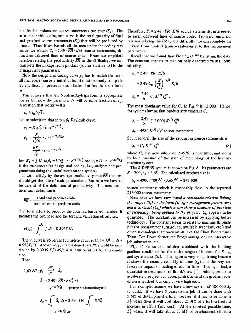
When the natural logarithm of the manpower divided by thecorresponding elapsed time is plotted against elapsed timesquared (Fig. 8), a straight line is produced in which In (Kftd)is the intercept and - 1/2 td is the slope.When this was done for some 100 odd systems, it was found

that the argument of the intercept Kitd, had a most interesting

in 1125)

L

in (5) _

in iY/t)J*

INTERCEPT = 1. K/td2)

~~~~~SLOPE = 1

t2 (years2I

Fig. 8. Difficulty versus time2 [291.

property. If the number K/t? was small, it corresponded witheasy systems; if the number was large, it corresponded withhard systems and appeared to fall in a range between theseextremes. This suggested that the ratio Kitd? represented thedifficulty of a system in terms of the programming effort andthe time to produce it.When this difficulty ratio (Kit2) is plotted against the pro-

ductivity (PR) for a number of systems we get the relation-ships shown in Fig. 9.This relationship is the missing link in the software process.

This can be illustrated by removing the cover from the blackbox, as shown in Fig. 10.

Feasible Effort-Time RegionA feasible software development region can be established

intuitively. Systems range in effort from 1 to 10 000 MY life-cycle. Development times (td) range from 1 or 2 months to5 to 6 years. For large systems, the range narrows to 2-5 yearsfor most systems of interest. Five years is limiting from aneconomic viewpoint. Organizations cannot afford to waitmore than 5 years for a system. Two years is the lower limitbecause the manpower buildup is too great. This can beshown a number of ways.

1) Brooks [1] cites Vysottsky's observation that large scalesoftware projects cannot stand more than a 30 percent per yearbuildup (presumably after the first year). The Rayleigh equa-tion meeting this criterion is with td > 2 years.2) The manpower rate invokes the intercommunication law

cited by Brooks [1]; complexity = N[(N- 1)/2] where Nisthe number of people that have to intercommunicate. Thus, ifthe buildup is too fast, effective human communication can-not take place because the complexity of these communica-tion paths becomes too great.3) Management cannot control the people on a large soft-

ware project at rates governed by the Norden/Rayleigh man-power equation with td < 2 years without heroic measures.4) Generally, internal rates of manpower generation (which

is a function of completion of current work) will not supportan extremely rapid buildup on a new project. New hiring canoffset this, but that approach has its own shortcomings.When the feasible region is portrayed in three dimensions by

introducing the difficulty Kitd? as the third dimension, we have

350


8 _5 t ; f +, t > - S ; 3, ,S lllstt0' ltitw PRODUCTI V ITY X;a6W < <X > WW1 g4 0 ~~~~~~~~~~~~~~DIFF1ICLTY. X4081 AVi!gH'~~~%LACS

. :ix .T 4 t ' iM'MS + S5 lll!lllo l||'!ll| 1 1 :

~~~~~4 | ASCOM1-SWt9<VADB t t X XWdi SAIL; AEwi6 0 - < 4 1+~~~~~~pms ,hR=1 O D'

3 tt X 1 , ..| 9 2 ili 'i!l''l < \ 1l'|S|AA| --2[ ;0 --fXX 1- Hf0 4414 ;Xi~~~~s0t-Xio :t L 0 :.; 0 , <CSLE X~~~VTAA

2 3 4 5 6 7 8 9 iOY 2 3 4 5

DIFFICULTY, D = K/td

Fig. 9. Productivity versus difficulty for a number of U.S. Army Computer Systems Command systems. Lines 1, 2, and 3represent different development environments. Line 1 represents a continental United States environment, batch jobsubmission, a consistent set of standards and for standard Army systems that would be used at many installations. Line 2is typical of a Pacific development environment, (initially) a different set of standards from 1, and the intended applica-tion was for one (or only a few) installations. Line 3 is typical of the European environment, different standards, singleinstallation application. The two points shown for lines 2 and 3 are insufficient in themselves to infer the lines. Othermore comprehensive data [14] show relations like line 1 with the same basic slope (-.6 2 to -.72). Based on this corrob-orating evidence, the lines 2 and 3 are sketched in to show the effect of different environment, standards, tools, andmachine constraints.

SOFTWARE DEVELOPMENT PROCESSl;INPUT 9BLACK BOX TRANSFORMATION OUTPUT

(K, td,O SS)MANPOWER

fl(K, t) 7 7 - \\

x~~~~~~~~~~DEEOPENT PR PR= 12000

(WHAT WE = K/ d2 TIME X PRPAY FOR) td (WHAT WE

Ss=fiPR)y1(t)dt GET-END__ vo g PRODUCT)

ENTROP S, = PR (.17K()?,

ABORTED KCOMPILES LOSSES (FUNCTION OF DIFFICULTY)

t ,'J) JJ. 1 (BLOOD, SWEAT, TEARS)JQ j fWHAT GETS GROUND UP IN THE PROCESS)

Fig. 10. Black box with cover removed.

a difficulty surface (Fig. 11). Note that as the developmenttime is shortened, the difficulty increases dramatically. Sys-tems tend to fall on a set of lines which are the trace of aconstant magnitude of the difficulty gradient. Each of theselines is characteristic of the software house's ability to do acertain class of work. The constants shown [81, [15], [27]are preliminary. Further work is needed to refine these anddevelop others.

Difficulty GradientWe can study the rate of change of difficulty by taking the

gradient of D. The unit vector ^1 points in td direction. Theunit vector 1 points in K (and $COST) direction.grad D points almost completely in the -i(-td) direction.

The importance of this fact is that shortening the developmenttime (by management guidance, say) dramatically increasesthe difficulty, usually to the impossible level.Plotting of U.S. Army Computer Systems Command systems

on the difficulty surface shows that they fall on three distinctlines:

Kftd3 = 8, K/td = 15, and K/td3 = 27.

The expression for gradD is

gradD= I + 23 2td t2(7)

We note that the magnitude of the t: component has the formK/td3. The magnitude of gradD is

Igrad D - a Dla td = 2K/td,.since a Dla K << a D1a td

throughout the feasible region. igrad D is the magnitude ofthe maximum directional derivative. This points in the nega-

351

1 2 3 4 5 6 7 8 9 1 2 3 4 5 6 7 8 9 1 2 3 4 5

n

2 3 4 5 6 7 8 9 l


LINE

/

Fig. 11. Difficulty surface.

tive i (td) direction. The trace of all such points is a line K =constant times td. Such a line seems to be the maximum diffi-culty gradient line that the software organization is capable ofaccomplishing. That is, as system size is increased, the develop-ment time will also increase so as to remain on the trace of aline having a constant magnitude of the gradient defined by

K/td = C, where C can equal either 8, 15, or 27. 2

Study of all U.S. Army Computer Systems Command sys-tems shows that 1) if the system is entirely new-has manyinterfaces and interactions with other systems-C 8; 2) if thesystem is a new stand-alone system, C _ 15; and 3) if the sys-tem is a rebuild or composite built up from existing systemswhere large parts of the logic and code already exist, thenC_ 27. (These values may vary slightly from software houseto software house depending upon the average skill level ofthe analysts, programmers, and management. They are, in asense, figures of merit or "leaming curves" for a softwarehouse doing certain classes of work.)

Significance ofManagement Directed Changes to theDifficultyManagers influence the difficulty of a project by the actions

they take in allocating effort (-K) and specifying scheduledcompletion (-td). We can determine the sensitivity of thedifficulty to management perturbation by considering a fewexamples.Assume we have a system which past experience has shown

2These constants are preliminary. It is very likely that 6 to 8 otherswill emerge as data become available for different classes of systems.

can be done with these parameter values: K = 400 MY, td = 3years. Then D = K/td2 = 400/9 = 44.4 MY/YR2. If manage-ment were to reduce the effort (life-cycle budget) by 10percent, then K = 360, MY td = 3 years, as before, and D =360/9 = 40 (10 percent decrease). However, the more com-mon situation is attempting to compress the schedule. Ifmanagement were to shorten the time by 2 year, then K = 400,td = 2.5, and D = 400/6.25 = 64 (44 percent increase). Theresult is that shortening the natural development time willdramatically increase the difficulty. This can be seen easily byexamining Fig. 6 and by noting that K = V'e)Ymax td. D isthus proportional to Ymax/td which is the slope from the originto the peak of the Norden/Rayleigh curves. If the slope is toogreat, management cannot effectively convert this increasedactivity rate into effective system work probably because ofthe sequential nature of many of the subprocesses in the totalsystem building effort.

V. THE SOFTWARE EQUATIONWe have shown that if we know the management parameters

K and td, then we can generate the manpower, instantaneouscost, and cumulative cost of a software project at any time tby using the Rayleigh equation.But we need a way to estimate K and td, or better yet, ob-

tain a relation that shows the relation between K, td, and theproduct (the total quantity of source code).

It can be shown that if we multiply the first subcycle curve(shown as the design and coding curve in Fig. 4) by the averageproductivity (PR) and a constant scale factor (2.49) to accountfor the overhead inherent in the defmition of productivity,then we obtain the instantaneous coding rate curve. Theshape of this curve is identical to the design and coding curve

352


but its dimensions are source statements per year (S). Thearea under this coding rate curve is the total quantity of finalend product source statements (SS) that will be produced bytime t. Thus, if we include all the area under the coding ratecurve we obtain S8 = 2.49 *PR *K/6 source statements, de-fined as delivered lines of source code. From our empiricalrelation relating the productivity PR to the difficulty, we cancomplete the linkage from product (source statements) to themanagement parameters.Now the design and coding curve A, has to match the over-

all manpower curve y' initially, but it must be nearly completeby td; thus, Y, proceeds much faster, but has the same formasy5.This suggests that the Norden/Rayleigh form is appropriate

for Y, but now the parameter to will be some fraction of td.A relation that works well is

to-tdl4-6

Let us substitute that into a %l Rayleigh curve,

A ,=K/t2 .t e.-t2/2t

Y1= e-t d21di

6KI e-3t2/t?j2td

but K1 = 6 K, sohl, K/t= * t 3t /td andyt =D t eis the manpower for design and coding, i.e., analysts and pro-grammers doing the useful work on the system.

If we multiply by the average productivity rate PR then weshould get the rate of code production. But here we have tobe careful of the definition of productivity. The most com-mon such definition is

total end product codePR = --

total effort to produce code

The total effort to produce the code is a burdened number-itincludes the overhead and the test and validation effort, i.e.,

tdY(td)= 9 dt = 0.3935 K.

The Pi curve is 95 percent complete at td ,yl (td) = ftd A, dt =0.95(K/6). Accordingly, the burdened rate PR should be mul-tiplied by 0.3935 K/0.95/6 K = 2.49 to adjust for this condi-tion.Then

2.49PR*i =dS= s

S8= 2.49 -PR K/tt - t

e-3t2/td source statements/year

0 0

. t -e-3tl dt.

Therefore, Ss = 2.49 -PR K/6 source statements, interpretedto mean delivered lines of source code. From our empiricalrelation relating the PR to the difficulty, we can complete thelinkage from product (source statements) to the managementparameters.Recall that we found that PR = Cn, D-2/3 by fitting the data.

The constant appears to take on only quantized values. Sub-stituting,

Ss = 2.49 * PR * K/6

-2494,~~2/= 2.49 Cn K16

The most dominant value for C,, in Fig. 9 is 12 000. Hence,for systems having that productivity constant C,,

= 6 (12000)K'13t4/3

Ss = 4980 K113 t4'3 source statements.d

So, in general, the size of the product in source statements is

S = CkK13 t413 (8)where Ck has now subsumed 2.49/6, is quantized, and seemsto be a measure of the state of technology of the human-machine system.The SIDPERS system is shown on Fig. 8. Its parameters are

K = 700, td = 3.65. The calculated product size is

Ss = 4980 (700)1/3 (3.65)4/3 = 247 000

source statements which is reasonably close to the reported256 000 source statements.Note that we have now found a reasonable relation linking

the output (SS) to the input (K, td - management parameters)and a constant (Ck) which is somehow a measure of the stateof technology being applied to the project. Ck appears to bequantized. The constant can be increased by applying bettertechnology. The constant seems to relate to machine through-put (or programmer turnaround, available test time, etc.) andother technological improvements like the Chief ProgrammerTeam, Top Down Structured Programming, on-line interactivejob submission, etc.

Fig. 12 shows this relation combined with the limitinggradient conditions for the entire ranges of interest for K, td,and system size (Ss). This figure is very enlightening becauseit shows the incompressibility of time (td) and the very un-favorable impact of trading effort for time. This is, in fact, aquantitative description of Brook's law [1]. Adding people toaccelerate a project can accomplish this until the gradient con-dition is reached, but only at very high cost.For example, assume we have a new system of 100 000 Ss

to build. If we have 5 years to the job, it can be done with5 MY of development effort; however, if it has to be done in34 years then it will cost about 25 MY of effort-a fivefoldincrease in effort (and cost). At the shortest possible time,23 years, it will take about 55 MY of development effort, a

353


SYSTEM SIZE SS (000)

(a)

700 800 900 1000Suu 4uu bEu

SYSTEM SIZE Ss (°°°)

(b)

Fig. 12. (a) Size-time-effort tradeoff for function Ss = 4984 K1/3 td/3. This is representative of about 5 years ago. Batchdevelopment environment, unstructured coding, somewhat "fuzzy" requirements and severe test bed machine constraint.(b) Size-time-effort tradeoff for function S. = 10040 K11/3 t413 This is reasonably representative of a contemporarydevelopment environment with on-line interactive development, structured coding, less "fuzzy" requirements, and ma-chine access fairly unconstrained. In comparing the two sets of curves note the signifilcant improvement in performancefrom the introduction of improved technology which is manifested in the constant Ck.

354

1, 443

siE

.M

DEV 5f MY6

5t

/ 01- _SIZE - TIME - EFFORTTRADE-OFF CHART

)Sr~~~~~~~~~~~~~~~~~~= 1/ L< 3S k Knn 4/3 ck = 10040

0

7

-0

41

J'

x

IlUU zUU bUU "I


tenfold increase over the 5 year plan. Clearly, time is not a"free good" and while you can trade people for time withinnarrow limits, it is a most unfavorable trade and is only justi-fied by comparable benefits or other external factors.

The Effort-Time TradeoffLawThe tradeoff law between effort and time can be obtained

explicity from the software equation

Ss = Ck K113 tH3

A constant number of source statements implies K td constant.So K = constant/td, or proportionally, development effort =constant/t4d, is the effort-development time tradeoff law.Note particularly that development time is compressible

only down to the governing gradient condition (see Fig. 12);the software house is not capable of doing a system in lesstime than this because the system becomes too difficult forthe time available.Accordingly, the set of curves relating development effort

(0.4 K), development time (td), and the product (Ss) permitsproject managers to play "what if" games and to tradeoffcost versus time without exceeding the capacity of the soft-ware organization to do the work.

Effect ofConstant ProductivityOne other relation is worth obtaining; the one where the

average productivity remains constant.

PR = C, D-213 = constant implies thatD = constant.

So the productivity for different projects will be the sameonly if the difficulty is the same. This does not seem reason-able to expect very frequently since the difficulty is a measureof the software work to be done, i.e., K/td =D which is afunction of the number of files, the number of reports, andthe number of programs the system has. Thus, planning a newproject based on using the same productivity a previous pro-ject had, is fallacious unless the difficulty is the same.The significance of this relation for an individual system is

that when the PR is fixed, the difficulty K/td remains constantduring development. However, we know that the difficulty isa function of the system characteristics, so if we change thesystem characteristics during development, say the number offiles, the number of reports, and the number of subprograms,then the difficulty will change and so will the average pro-ductivity. This in turn will change our instantaneous rate ofcode production (S3) which is made up of both parameterterms and time-varying terms.In summary then, Ss = Ck K113 t4/3 appears to be the manage-

ment equation for software system building. As technologyimproves, the exponents should remain fixed since they re-late to the process. Ck will increase (in quantum jumps) withnew technology because this constant relates to the overallinformation throughput capacity of the system and (tenta-tively) seems to be more heavily dependent on machinethroughput than other factors.

The Software Differential EquationHaving shown some of the consequences of the Rayleigh

equation and its application to the software process let us ex-

amine why we have selected this model rather than a numberof other density functions that could be fitted to the data. Wereturn to Norden's initial formulation to obtain the differen-tial equation.Norden's description [8J of the process is this: The rate of

accomplishment is proportional to the pace of the work timesthe amount of work remaining to be done. This leads to thefirst-order differential equation

. = 2at (K - y)where j is the rate of accomplishment, 2at is the "pace" and(K - y) is the work remaining to be done. Making the explicitsubstitution for a = (1/2td) we have j = t/td (K - y). t/t2 isNorden's linear learning law.We differentiate once more with respect to time, rearrange,

and obtain

(9)

This is a second derivative form of the software equation.The Norden/Rayleigh integral is its solution which can beverified by direct substitution. Note that this equation issimilar to the nonhomogeneous 2nd order differential equa-tions frequently encountered in mechanical and electricalsystems. There are two important differences. The forcingfunction D = K/tdi is a constant rather than the more usualsinusoid, and the _j term has a variable coefficient t/td, pro-portional to the 1st power of time.

Uses Of the Software EquationThe differential equation J + t/t2 y + y/t2 = K/td is very

useful because it can be solved step-by-step using the Runge-Kutta solution. The solution can be perturbed at any pointby changing K/td = D, the difficulty. This is just what happensin the real world when the customer changes the requirementsor specifications while development is in process. If we havean estimator for D (which we do) that relates K/td to the sys-tem characteristics, say the number of files, the number ofreports, and the number of application programs, then we cancalculate the change in D and add it to our original D, con-tinue our Runge-Kutta solution from that point in time andthus study the time slippage and cost growth consequences ofsuch requirements changes. Several typical examples are givenin [131.When we convert this differential equation to the design and

coding curve j1 by substituting td/\f6, and K1 =K/6, weobtain

.. 6tl

6 Kd 2t 2td td2' td

(10)

and multiplying this by the PR and conversion factor as beforewe obtain an expression that gives us the coding rate and cumu-lative code produced at time t.

is + tI(td/INf6)2 Ss + lI(td/V6)2 SS = 2.49 PR- K/tlt=Cn(Ka td)a1a3= 2.49 CnD'13. (I11)

Since D is explicit, this equation can also be perturbed at any

355

tltd2 2 = Kltd.. + yltd 2 =D.


TABLE IRUNGE-KUTTA SOLUTION TO CODING RATE DIFFERENTIAL EQUATION

FOR SIDPERS

t (years)

0

.51.01.5

2.0

2.53.03.5

-0 3.65

4.04.55.0

Coding Rate(Ss/year)

(000)

0

52.889.2101.090.868.444.224.920.3312.35.362.09

Cumulative Code(SS)(000)

0

13.650.098.6

147.0187.0

215.0323.0236.0 4- Actual size241.0 at extension

is 256,000 S246.0 which is

247.0 pretty closeto this

SIDPERS parameters

K = 700 MYtd = 3.65 yearsD = 52.54 MY/yrPR = 914 S /MY (burdened)

DIFFERENTIAL EQUATION

S + ___t_ __ S + _ _1 S = 2.49. FI D = 2.49.(12009D-2 3).D3.651 2 13.65 2 = 2.49 (12009) (D)1/3

46}E y = 29902 (52.54)1/3= 111785

time t in the Runge-Kutta solution and changes in require-ments studied relative to their impact on code production.An example of code production for SIDPERS using the

Runge-Kutta solution is shown in Table I.This equation in both its manpower forms y and _YR as well

as the code form can be used to track in real-time manpower,cumulative effort, code production rate, and cumulative code.Since the equation relates to valid end product code and doesnot explicitly account for seemingly good code that later getschanged or discarded, actual instantaneous code will probablybe higher than predicted by the equation. Thus, a calibrationcoefficient should be determined empirically on the firstseveral attempts at use and then applied in later efforts wheremore accurate tracking and control are sought.

VI. SIZING THE SOFTWARE SYSTEMHaving justified the use of the Rayleigh equation from

several viewpoints, we turn to the question of how we can

determine the parameters K and td early in the process-specifically during the requirements and specification phasebefore investment decisions have to be made.One approach that works in the systems definition phase

and in the requirements and specification phase is to use thegraphical representation of the software equation Ss = Ck K113t4/3 as in Fig. 12. Assume we choose Ck using criteria as out-lined in Fig. 12. It is usually feasible to estimate a range ofpossible sizes for the system, e.g., 1500 000 to 2500 000 Ss. Itis also possible to pick the range of desired development times.

These two conditions establish a probable region on the trade-off chart (Fig. 12(b), say). The gradient condition establishedthe limiting constraint on development time. One can thenheuristically pick most probable values for development timeand effort without violating constraints, or one can even simu-late the behavior in this most probable region to generate ex-pected values and variances for development time and effort.The author uses this technique on a programmable pocketcalculator to scope projects very early in their formulation.Another empirical approach is to use a combination of prior

history and regression analysis that relates the managementparameters to a set of system attributes that can be deter-mined before coding starts. This approach has produced goodresults.Unfortunately, K and td are not independently linearly re-

lated to such system attributes as number of files, number ofreports, and number of application programs. However, K/td =D is quite linear with number of files, number of reports, andnumber of application subprograms, both individually andjointly. Statistical tests show that number of files and numberof reports are highly redundant so that we can discard one andget a good estimator from the number of application subpro-grams and either of the other two.There are relationships other than the difficulty that have

significantly high correlation with measures of the product.These relationships are

Klt3 =f2(X1,X2,X3)

K/td =f3(xI,x2,x3)Klt = f4(Xi,X2,X3)K= f5 (x1,x2,X3)

Ktd = f6(x1,x2,x3)

Ktd =f7(xI,x2,x3)where K and td are the parameters of the Norden/Rayleighequation. xi is the number of files the system is expected tohave, x2 is the number of reports or output formats the sys-tem will have, and X3 is the number of application subpro-grams. These independent variables were chosen becausethey directly relate to the program and system building pro-cess, that is, they are representative of the programmer andanalyst work to create modules and subprograms. More im-portantly, they are also a measure of the integration effortthat goes on to get programs to work together in a systemsprogramming product. The other important reason for usingthese variables is practical: they can be estimated with reason-able accuracy (within 10-15 percent) early enough in therequirements specification process to provide timely man-power and dollar estimates. Note also that X1, X2, X3 areimprecise measures-the number of subprograms, say-thisimplies an average size of an individual program with someuncertainty or "random noise" present. It seems prudent tolet the probability laws help us rather than try to be too pre-cise when we know that there are many other random-likeperturbations that will occur later on that are unknown to us.For business applications, the number of files, reports, andapplication subprograms work very well as estimators. For

356


TABLE IIUSACSC SYSTEM CHARACTERISTICS

Number of

System Life Cycle Size Development Time Files Rpts. Appl. Progs.K (MY) td (YRS) xl x2 X3

MPMIS 73.6 2.28 94 45 52

MRM 84 1.48 36 44 31

ACS 33 1.67 11 74 39

SPBS 70 2.00 8 34 23

COMIS 27.5 1.44 14 41 35

AUDIT 10 2.00 11 5 5

CABS 7.74 1.95 22 14 12

MARDIS 91 2.50 6 10 27

MPAS 101 2.10 25 95 109

CARMOCS 153 2.64 13 109 229

SIDPERS 700 3.65 172 179 256

VTAADS 404 3.50 155 101 144

BASOPS-SUP 591 2.73 81 192 223

SAILS AB/C 1028 4.27 540 215 365

SAILS ABlX 1193 3.48 670 200 398

STARCIPS 344 3.48 151 59 75

STANFINS 741 3.30 270 228 241

SAAS 118 2.12 131 152 120

COSCOM 214 4.25 33 101 130

other applications other estimators should be examined. It isusually apparent from the functional purpose of the systemwhich estimators are likely to be best.The dependent variables K/td ... K, Ktd, Ktd also have sig-

nificance. K/t3 is proportional to the difficulty gradient, K/tdiis the difficulty, a force-like term which is built into our time-varying solution model, the Rayleigh equation. KItd is pro-portional to the average manpower of the life-cycle and K isthe life- cycle size (area under Rayleigh manpower curve).Ktd is the "action" association with the action integral, and

Ktd is a term which arises when the change in source state-ments is zero.A numerical procedure to obtain estimators for the various

Ktd, Ktd, K ... K/td terms is to use multiple regression analy-sis and data determined from the past history of the softwarehouse. A set of data from U.S. Army Computer SystemsCommand is shown in Table II.We will determine regression coefficients from x2, X3 to

estimate KItd as an example of the procedure. We write anequation of the form

a2X2 + aL3X3 = KItdfor each data point (K/td, x2, X3) in the set. This gives a setof simultaneous equations in the unknown coefficient *2 anda3 . We solve the equations using matrix algebra as follows:

[X] T [X] [C] = [XI T [K/td] (12)[a] = ([XI T [XI )1 [X]T [Kltd] (13)

a2 [C22 C23 -'[Klt -X2

a3] [C32 C33 J [;KItd * X3](14)

where the a matrix is a single column vector of 2 elements,the X matrix is a matrix ofN rows and 2 columns, the X-1 in-verse matrix is a square matrix of 2 rows and 2 columns, andthe 2KItdi - x matrix is a column vector of two elements.Solving for the ai provides coefficients for the regression esti-mator. For the data set of Table II, we obtain

KItd = 0.2200 x2 + 0.5901 X3.

Estimators for each of the other Kftd3 . . K, Ktd, Ktd4 aredetermined in the same way. These estimators for the data setof Table II are listed below:

K/td = 0.1991 x2 + 0.0859 X3

KItd = 0.2200 x2 + 0.5901 X3

K = -0.3447 x2 + 2.7931 X3

Ktd =-4.1385x2 + 11909x3

Ktd = -483.3196x2 + 791.0870 X3.

Assuming we have estimates of the number of reports andthe number of application subprograms, we can get estimatesofK and td by solving any pair of these equations simultane-ously, or we can solve them all simultaneously by matrixmethods.Since we have observed that different classes of systems tend

357


K(MY)

10 100 1000 10000NO. OF APPLICATION PROGRAMS

Fig. 13. Life-cycle size as a function of number of application pro-grams and number of reports.

to fall along distinct constant difficulty gradient lines, we canexploit this feature by forcing the estimators to intersect withsuch a predetermined constant gradient line. We can illustrateusing the matrix approach. For example, let us assume wehave a new stand-alone system with an estimate from the speci-fication that the system will require 179 reports and 256 appli-cation programs. The gradient relation for a stand-alone is

K/td = 14.

The regression estimators are

K/4 = 57.63

Kltd = 190.45

K = 652.54

Ktd = 2307.91

Ktd =116 004.76.

Taking natural logarithms of these six equations we obtainthe matrix equation

[1 11 1 1 16l-3 -2 -1 0 1 4

1 -31 -2

1 -1

1 0

1 1

14

which yields

InK =6.5189;K 677.86 MY

In td = 1.2772;rd 3.59 YRS.

The data used for these examples are that of SIDPERS (K =700, td = 3.65, as of 1976). The estimators perform quitewell in this general development time and size regime. Theyare less reliable and less valid for small systems (K < 100 MY;td < 1.5 years) because the data on the larger systems are moreconsistent. Extrapolation outside the range of data used togenerate the estimators is very tenuous and apt to give badresults.Once the estimating relationships have been developed for

the software house as just outlined above, then they can berun through the range of likely input values and system typesto construct some quick estimator graphs. An example of anearly set of quick estimator charts for U.S. Army ComputerSystems Command is shown in Figs. 13-15. These figures giveconsiderable insight into the way large scale software projects

2.6391

4.0540

5.2494

6.4809

7.7441

11.6614

358

In K.

I 1 1 1 1 CIn td --3 -2 -1 0 1 4

-


10000

1 000

K(MY)

100

10

0 100 1000 10000NO. OF APPLICATION PROGRAMS

Fig. 14. Life-cycle size as function of number of application programsand number of reports.

td (YRS)

50 100 150 200 250 300 350 400 450 500NO. OF APPLICATION PROGRAMS

Fig. 15. Development time as a function of number of application programs and number of reports.

have to be done in terms of number of application programs,reports, and the effort to integrate these pieces of work.Can the estimators developed here be used by other soft-

ware houses? Probably not-at least not without great careand considerable danger. This is because each software househas its own standards and procedures. These produce differ-ent average lengths of application programs. Accordingly,another software house might have an average length of pro-gram of 750 lines of Cobol compared with about 1000 lines of

Cobol for Computer Systems Command. Thus, the numberof application programs would reflect a different amount ofwork/per application program than CSC experience. Scalingwould be necessary. Scaling may or may not be linear. Thereis no evidence to suggest scaling should be linear since mosteverything else in the software development process is somecomplex power function. Furthermore, we have shown earlierthe influence of the state-of-technology constant. The multipleregression technique does not explicitly account for this; it is

359

1-


implicit within the data. Therefore, the regression analysis hasto be done for each software house to account for those fac-tors which would be part of a state-of-technology constant.

Engineering and Managerial ApplicationSpace does not permit the development of management engi-

neering applications of these concepts to planning and con-

trolling the software life-cycle. The applications have beenrather comprehensively worked out and are contained in [131.Error analysis, or determining the effect of stochastic variation,again has not been treated due to space limitations.

VII. SUMMARYSoftware development has its own characteristic behavior.

Software development is dynamic (time varying)-not static.Code production rates are continuously varying-not con-

stant.The software state variables are

1) the state of technology C,n or Ck;2) the applied effort K;3) the development time td; and4) the independent variable time t.The software equation relates the product to the state

variables:

00Ss= PR -

y, dt =CkKd13t1

The tradeoff law K= Clt?4 demonstrates the cost of tradingdevelopment time for people. Time is not free. It is very

expensive.

REFERENCES

[1] F. P. Brooks, Jr., The Mythical Man-Month. Reading, MA:Addison-Wesley, 1975.

[21 L. H. Morin, "Estimation of resources for computer programmingprojects," M.S. thesis, Univ. North Carolina, Chapel Hill, NC,1973.

[31 P. F. Gehring and U. W. Pooch, "Software development manage-ment," Data Management, pp. 14-18, Feb. 1977.

141 P. F. Gehring, "Improving software development estimates oftime and cost," presented at the 2nd Int. Conf. Software Eng-neering, San Francisco, CA, Oct. 13, 1976.

[51 -, "A quantitative analysis of estimating accuracy in softwaredevelopment," Ph.D. dissertation, Texas Univ., College Station,TX, Aug. 1976.

[6] J. D. Aron, "A subjective evaluation of selected program develop-ment tools," presented at the Software Life Cycle ManagementWorkshop, Airlie, VA, Aug. 1977, sponsored by U.S. ArmyComputer Systems Command.

[7] P. V. Norden, "Useful tools for project management," in Manage-ment of Production, M. K. Starr, Ed. Baltimore, MD: Penguin,1970, pp. 71-101.

[81 -, "Project life cycle modelling: Background and applicationof the life cycle curves," presented at the Software Life CycleManagement Workshop, Airlie, VA, Aug. 1977, sponsored byU.S. Army Computer Systems Command.

[91 L. H. Putnam, "A macro-estimating methodology for softwaredevelopment," in Dig. of Papers, Fall COMPCON '76, 13th IEEEComputer Soc. Int. Conf., pp. 138-143, Sept. 1976.

[101 -, "ADP resource estimating: A macro-level forcasting method-ology for software development," in Proc. 15th Annu. U.S.Army Operations Res. Symp., Fort Lee, VA, pp. 323-327, Oct.26-29, 1976.

f111 -, "A general solution to the software sizing and estimatingproblem," presented at the Life Cycle Management Conf. Amer.Inst. of Industrial Engineers, Washington, DC, Feb. 8, 1977.

[121 -, "The influence of the time-difficulty factor in large scale

software development," in Dig. of Papers, IEEE Fall COMPCON'77 15th IEEE Computer Soc. Int. Conf., Washington, DC, pp.348-353, Sept. 1977.

[131 L. H. Putnam and R. W. Wolverton, "Quantitative management:Software cost estimating," a tutorial presented at COMPSAC'77, IEEE Computer Soc. 1st Int. Computer Software andApplications Conf., Chicago, IL, Nov. 8-10, 1977.

1141 C. E. Walston and C. P. Felix, "A method of programmingmeasurement and estimation," IBM Syst. J., vol. 16, pp. 54-73, 1977.

[151 E. B. Daly, "Management of software development," IEEETrans. Software Eng., vol. SE-3, pp. 229-242, May 1977.

1161 W. E. Stephenson, "An analysis of the resources used in thesafeguard system software development," Bell Lab., draft paper,Aug. 1976.

1171 "Software cost estimation study: Guidelines for improved costestimating," Doty Associates, Inc., Rome Air DevelopmentCenter, Griffiss AFB, NY, Tech. Rep. RADC-TR-77-220, Aug.1977.

[181 G. D. Detletsen, R. H. Keer, and A. S. Norton, "Two genera-tions of transaction processing systems for factory control,"General Electric Company, internal paper, undated, circa 1976.

[191 "Software systems development: A CSDL project history," theCharles Stark Draper Laboratory, Inc., Rome Air DevelopmentCenter, Griffiss AFB, NY, Tech. Rep. RADC-TR-77-213, June1977.

[20] T. C. Jones, "Program quality and programmer productivity,"IBM Syst. J., vol. 17, 1977.

1211 "Software systems development: A CSDL project history," theCharles Stark Draper Laboratory, Inc., Rome Air DevelopmentCenter, Griffiss AFB, NY, Tech. Rep. RADC-TR-77-213, June1977.

[221 A. D. Suding, "Hobbits, dwarfs and software," Datamation,pp. 92-97, June 1977.

[23] T. J. Devenny, "An exploratory study of software cost esti-mating at the electronic systems division," Air Force Inst. ofTechnology, WPAFB, OH, NTIS AD-A1030-162, July 1976.

[241 D. H. Johnson, "Application of a macro-estimating methodologyfor software development to selected C group projects," NSA,internal working paper, May 6, 1977.

1251 J. R. Johnson, "A working measure of productivity," Datamation,pp. 106-108, Feb. 1977.

[261 R. E. Merwin, memorandum for record, subject: "Data processingexperience at NASA-Houston Manned Spacecraft Center,"Rep. on Software Development and Maintenance for Appollo-GEMINI, CSSSO-ST, Jan. 11, 1970.

[271 B. P. Lientz, E. B. Swanson, and G. E. Tompkins, "Characteristicsof application software maintenance," Graduate School ofManagement, UCLA, DDC ADA 034085, 1976.

[281 R. E. Bellman, "Mathematical model making as an adaptiveprocess," ch. 17, in Mathematical Optimization Techniques,The Rand Corporation, R-396-PR, Apr. 1963.

[29] G. E. P. Box and L. Pallesen, "Software budgeting model," Mathe-matics Research Center, University of Wisconsin, Madison, (Feb.1977 prepublication draft).

[30] "Management Information Systems," A Software ResourceMacro-Estimating Procedure, Hq. Dep, of the Army, DA Pam-phlet 18-8, Feb. 1977.

[311 A. M. Pietrasanta, "Resource analysis of computer programsystem development," in On the Management of ComputerProgramming, G. F. Weinwurn, Ed. Princeton, NJ: Auerbach,1970, p. 72.

Lawrence H. Putnam was born in Massachusetts. He attended the Uni-versity of Massachusetts for one year and then attended the U.S.Military Academy, West Point, NY, graduating in 1952. He was com-missioned in Armor and served for the next 5 years in Armor andInfantry troop units. After attending the Armor Officer AdvancedCourse, he attended the U.S. Naval Post Graduate School, Monterey,CA, where he studied nuclear effects engineering for 2 years, gradu-ating in 1961 with the M.S. degree in physics. He then went to the

360


Combat Developments Command Institute of Nuclear Studies, wherehe did operations research work in nuclear effects related to targetanalysis, casualty, and troop safety criteria. Following a tour in Korea,he attended the Command and General Staff College.Shortly thereafter he returned to nuclear work as a Senior Instructor

and Course Director in the Weapons Orientation Advanced Course atField Command, Defense Nuclear Agency, Sandia Base, NM. Follow-ing that, he served in Vietnwn with the G4, I Field Force, commandeda battalion at Fort Knox, KY, for 2 years, and then spend 4 years in the

Office of the Director of Management Information Systems and As-sistant Secretary of the Army at Headquarters, DA. His final tour ofactive service was with the Army Computer Systems Command as

Special Assistant to the Commanding General. He retired in the gradeof Colonel. He is now with the Space Division, Information SystemsPrograms, General Electric Company, Arlington, VA. His principalinterest for the last 4 years has been in developing methods and tech-niques for estimating the life-cycle resource requirements for majorsoftware applications.

361

a general empirical solution to macro software sizing and estimating ... · sizing and estimating...

Documents