a general formulation for the stiffness matrix of parallel
TRANSCRIPT

HAL Id: hal-00759074https://hal.archives-ouvertes.fr/hal-00759074
Preprint submitted on 5 Dec 2012
HAL is a multi-disciplinary open accessarchive for the deposit and dissemination of sci-entific research documents, whether they are pub-lished or not. The documents may come fromteaching and research institutions in France orabroad, or from public or private research centers.
L’archive ouverte pluridisciplinaire HAL, estdestinée au dépôt et à la diffusion de documentsscientifiques de niveau recherche, publiés ou non,émanant des établissements d’enseignement et derecherche français ou étrangers, des laboratoirespublics ou privés.
A General Formulation for the Stiffness Matrix ofParallel Mechanisms
Cyril Quennouelle, Clément M. Gosselin
To cite this version:Cyril Quennouelle, Clément M. Gosselin. A General Formulation for the Stiffness Matrix of ParallelMechanisms. 2009. �hal-00759074�

A General Formulation
for the Stiffness Matrix of Parallel Mechanisms
Cyril Quennouelle∗
Clement Gosselin
Laboratoire de robotique,Departement de genie mecanique, Universite Laval
1065, avenue de la medecine - Quebec, QC, Canada - G1V 0A6
Abstract
Starting from the definition of a stiffness matrix, the authors present a new formula-
tion of the Cartesian stiffness matrix of parallel mechanisms. The proposed formulation
is more general than any other stiffness matrix found in the literature since it can take
into account the stiffness of the passive joints, it can consider additional compliances
in the joints or in the links and it remains valid for large displacements. Then, the
validity, the conservative property, the positive definiteness and the relation with other
formulations of stiffness matrices are discussed theoretically. Finally, a numerical ex-
ample is given in order to illustrate the correctness of this matrix.
1 Introduction
A robotic manipulator is a mechanism designed to displace objects in space or in a plane.Therefore, a high precision in the position and orientation of the end-effector and a goodrepeatability of motion are desirable properties of a manipulator. To fulfil this objective, anaccurate model of the mechanism is required. In particular, it is important to be able toprecisely characterize the stiffness of the manipulator, i.e., to determine the relation betweenthe loads applied to the mechanism and the resulting displacements. The mathematicalobject most commonly used to characterize the stiffness of a mechanism is the stiffnessmatrix.
In the literature, numerous papers deal with the stiffness matrix (SM) of robotic manipu-lators (See section 2). However, to the best knowledge of the authors, none of them presents
∗Corresponding author
1

a SM that is general and valid for any parallel mechanism (PM), notably, PMs with passivejoints that have a non zero stiffness and where some additional compliances (in the jointsas well as in the rigid links) are taken into account. The latter correspond to elasticallyarticulated rigid-body systems [1] or compliant mechanisms [2] (notably when the compliantjoints are modelled using a multi-degree of freedom (DOF) pseudo-rigid body model [3]).Since such a matrix is essential for the quasi-static [4] and the dynamic modelling of thesemechanisms, a SM is presented in this paper that considers the external loads, the changesof geometry of the mechanism, the stiffness of actuated and passive joints and even the finitestiffness of the rigid links, for both planar and spatial PMs.
After an overview of the literature on the SM, the kinematic model of a PM that takesinto account the passive joints is recalled. Then, expressions of the potential energy arederived in order to obtain the generalized stiffness matrix (GSM) of a PM and a general andmeaningful form of its Cartesian stiffness matrix (CSM). The properties of this matrix arethen discussed and finally, an application using the CSM is presented in order to illustratethe correctness and the possible applications of the presented matrix.
2 The Stiffness Matrix in the Literature
Definition Usually, a SM is mathematically defined as the Hessian matrix of a potential,i.e., the square matrix of second-order partial derivatives of this potential. For example, theCSM of a planar mechanism is the Hessian of the potential ξf associated to a wrench f withrespect to the Cartesian coordinates. It is written as
KC =d2ξfdx2
c
, (1)
where dxc represents a infinitesimal variation of the pose. However in many cases, such apotential energy cannot be determined and the latter definition cannot be applied. The SMis then defined as the Jacobian matrix of a wrench. This is written as
KC =df
dxc. (2)
It can be noticed that, when the associated potential is known, the conservative wrench isequal to the gradient of ξf , and both definitions are equivalent1.
Surprisingly, the SM of a mechanism submitted to an external load is symmetric onlywhen it is written in a coordinate basis [5–12]. It is asymmetric otherwise. Chen and Kaoadd in [13–17], that a SM is conservative, i.e., the work done by a force resulting from thismatrix along a closed path must be equal to zero. Finally, the Hessian matrix of a potentialbeing used to determine the stability of an equilibrium [9,18–20], a SM can be either positive-definite (or semi-definite) in a stable equilibrium or not in an unstable position.
1In the literature, it is sometimes stated that a wrench is equal to the opposite of the gradient (f = −∇ξf )and that a stiffness is equal to the opposite of the Jacobian matrix of a wrench (K = −∇f). These definitionslead to the same results.
2

Literature review In 1980, Salisbury was the first to formulate a SM for serial mechanismsin [21]. Then, the formula was extended to PMs in which only the stiffness of the actuatorswas considered [22, 23]. In fact, both matrices —which are still often accepted and appliednowadays—, are only valid in very particular conditions, pointed out by Chen, Kao et al.in [13–15]: they are correct only when the external loads are zero or when the Jacobianmatrix of the mechanism is constant. The misconception stems from the improper use ofthe following equations:
δx = Jδψf = KCδx
}
(3)
where f is the vector of the external loads, δψ a small displacement of the joints, J theJacobian matrix of the mechanism and δx a small displacement of the effector in the firstequation and a small gap of pose in the second equation. When both equations are usedtogether, a small gap and a small displacement are incorrectly considered as equivalent andthe second equation becomes inconsistent: when the external load remains constant, thereshould be no displacement of the mechanism.
The SM proposed by Chen, Kao et al. in [13] is correct for both serial and parallel planarmechanisms and it has been extended to spatial mechanisms in [17]. Using screw theory,Griffis and Duffy also noted the influence of an external load on the SM [24]. However, theproposed matrices still suffer from some lack of generality: they cannot take into accountthe stiffness of the passive joints and the degree of mobility (DOM) of the mechanism hasto be equal to the DOF of its end-effector platform. This results in a loss of accuracy in themodelling of compliant mechanisms.
In [25, 26], Zhang and Gosselin studied PMs with a constraining leg whose complianceswere modelled as virtual joints. Thus, the SM that they proposed considers the stiffness ofsome passive joints. However, they did not describe the effects of the external load nor theeffect of the internal force. Furthermore, their SM is not formulated in a general way andcan only be applied to the type of PMs with a constraining passive leg. Finally, some workshave been published that use a SM approaching the one presented in this paper, howeverwithout mainly focusing on it. For example, [27] considers a redundant actuation and [28]considers the stiffness of the passive joints .
3 Model of a Parallel Mechanism
3.1 Geometric Constraint
In a PM, the closure of the loops formed by the legs defines c geometrical constraints that haveto be satisfied by the joint coordinates. However, since these constraints can be dependentin the case of an overconstrained mechanism, the actual number of independent geometricconstraints is C (C ≤ c). The constraints are written as
K(θ) = 0C, (4)
where θ is the joint coordinate vector of the mechanism, including all joints, actuated andpassive. Note that the flexibility of the links and actuators can be taken into account by
3

adding virtual elastic joints in the mechanism [25, 26, 29]. These additional coordinates arealso included in vector θ.
3.2 Generalized Coordinates
A vector of generalized coordinates ψ, is defined such that λ the vector of the kinematicallydependent coordinates and θ, the complete joint coordinate vector of the mechanism, alwayssatisfy the geometric constraints. One has:
λ = λ(ψ) and θ = θ(ψ) (5)
where λ = [λ1; · · · ;λC]T and θ = [θ1; · · · ; θm]
T withm the number of joints in the mechanismand θk the coordinate associated with the kth joint. The dimension M of vector ψ equalsthe number of DOM of the (kinematically equivalent) mechanism, such that M+ C = m.
Structure of vector θ: The dependent and the generalized coordinates can be chosenarbitrarily. They can correspond to joint coordinates or to functions of the latter. If jointcoordinates are chosen as dependent and generalized coordinates, they can be sorted suchthat θ can be written as θT =
[
ψT ;λT]
.
3.3 Kinematic Constraints
The variation of the kinematically dependent joint coordinates is described by a matrix G
and a matrix R defined as
G =dλ
dψand R =
dθ
dψ=
[
1M
G
]
(6)
where 1M stands for the (M ×M) identity matrix. The above matrices represent the kine-matic constraints in a PM. The relations between the variation of the joint coordinates andthe variation of the generalized coordinates are expressed as
dλ = Gdψ and dθ = Rdψ. (7)
3.4 Kinematic Model
3.4.1 Pose of the Platform
The pose of the platform, represented by a set of parameters x, is defined as the averagepose of the end-effector of all legs of the mechanism. For the ith leg, the latter is writtenas xTi =
[
cTi ;qTi
]
, ci being the position vector of a chosen point on the platform and qi a setof parameters representing the orientation. The legs of the PM are indexed from a to n.
In a planar mechanism, qi is an angle along the z-axis; in a translational spatial mech-anism, the orientation is constant thus qi is not used; and in the general 6-DOF spatialcase, qi is a quaternion vector describing the orientation of the platform.
4

3.4.2 Variation of the Pose of the Platform
The instantaneous Cartesian variation of the pose of the platform is represented by a vector tdefined as tT =
[
vT ;ωT]
, v being the velocity of a chosen point of the platform and ω itsangular velocity. In a planar mechanism, t is equal to the instantaneous variation of thepose x, i.e., v = p and ω = q. But in the spatial case, since the angular velocity ω is a3-coordinate vector, a 3 × 4 matrix Λ is used to determine ω as a function of the variationof the quaternion vector q (See [30]). Defining a 6 × 7 matrix L, the variation of the posecan be written as
t = Lx, where L =
[
1 0
0 Λ
]
. (8)
An infinitesimal Cartesian variation of the pose dxc can also be defined as
dxc = tdt = Ldx, (9)
where dt represents an infinitesimal period of time. In the planar case, dxc = dx but in thespatial case, dxc has 6 components, while dx has 7 components.
3.4.3 Cartesian Kinematic model
The Jacobian matrix Jθ of a PM in which all joints —even the passive ones— are consideredis defined in [4] as the Jacobian matrix of the Cartesian pose with respect to the jointcoordinates. It is written as
Jθ =dxcdθ
. (10)
This matrix is actually composed of the columns of matrices Jθa to Jθn , the Jacobian matricesof each of the legs considered as an independent serial mechanism.
The Jacobian matrix of the pose of the end-effector with respect to the generalizedcoordinates is noted J and is defined as
J =dxcdψ
. (11)
The Cartesian kinematic model of the mechanism is written as
t = Jθθ = JθRψ = Jψ. (12)
3.4.4 Complete Kinematic Model
In a mechanism, especially in a compliant one, the number of DOM M can be larger thanthe number of degrees of freedom F of the end-effector platform [3, 29], thus determiningonly t may not be sufficient to completely determine the configuration of the mechanism.Therefore, t comprising F components, (M − F) additional output coordinates are chosento complete the kinematic model. They are noted yi and assembled in a vector y. Thesecoordinates can be any Cartesian coordinates of others points of the mechanism as wellas joint coordinates. By assembling all the yi and the F components of t in a vector u
containing M components, the direct complete kinematic model can be written as
u =
[
t
y
]
=
[
J
Jy
]
ψ = Hψ, (13)
5
where H is theM×M complete Jacobian matrix of the mechanism and Jy is the (M−F)×MJacobian matrix of the yi coordinates with respect to the generalized coordinates.
Inverse Kinematic Model In a non singular configuration, H is invertible. Then, fromequation (13), the inverse kinematic model of the mechanism is expressed as :
ψ = H−1u. (14)
When M = F, no additional coordinates yi are required, thus u = t and H = J. In thiscase, equation (14), can be written as
ψ = J−1t. (15)
Infinitesimal Variation With the infinitesimal variation of the pose and of the yi coor-dinates, the complete direct and inverse kinematic model are respectively written as
[
dxcdy
]
= Hdψ and dψ = H−1
[
dxcdy
]
. (16)
4 Stiffness Matrix of a Parallel Mechanism
4.1 Potential Energy of a Mechanism
4.1.1 Elastic Potential Energy
The potential energy stored in the elastic joints of a mechanism, noted ξθ, is written as
ξθ =
∫ θ
θ0
τ Tθ dθ =
∫ ψ
ψ0
τ Tψdψ +
∫ λ
λ0
τ Tλdλ (17)
where τ j is the vector of joint torques/forces associated with the joints corresponding tovector j and where θ0, ψ0
and λ0 correspond to the undeformed configurations of the joints.In the particular —but frequent— case of elastic joints with constant stiffness, the potentialenergy is written as
ξθ =1
2∆ψTKψ∆ψ +
1
2∆λTKλ∆λ, (18)
with ∆ψ = ψ −ψ0and ∆λ = λ− λ0 and where Kψ and Kλ are the (diagonal) joint SMs.
4.1.2 Conservative External Load
In a planar mechanism, the potential energy ξf associated to the load f applied to theend-effector platform is equal to
ξf =
∫
x
x0
fTdxc =
∫
x
x0
fTJdψ, (19)
where x0 corresponds to the unloaded configuration.
6

In the spatial case since the angular velocity ω and the infinitesimal variation of pose dxcare not integrable, the associated potential cannot be written. However, the instantaneouspower of a 6-dimensional external load is defined as
ξf = fTl v +mTω = fT t = fTJψ, (20)
where fT =[
fTl ;mT]
, fl representing the 3-dimensional force vector and m the 3-dimensionalmoment vector.
4.1.3 Potential Energy of the Mechanism
In a planar mechanism, the potential energy ξf due to the external wrench is equal —apartfrom a constant ξ0— to the energy stored in the mechanism (ξf = ξθ+ ξ0). Using eq.(7) andeq.(19), this can be written as
∫ ψ
ψf0
fTJdψ =
∫ ψ
ψf0
τ Tψdψ +
∫ ψ
ψf0
τ TλGdψ + ξ0, (21)
where ξ0 represents the energy stored in the mechanism in configuration ψf0, where f = 0.This energy is not zero when a preload exists in the compliant joints. The infinitesimalvariation of eq.(21) is also valid for a spatial mechanism. It is written as
fTJdψ = τ Tψdψ + τ TλGdψ. (22)
4.2 Static Equilibrium
Differentiating eq.(21) with respect to the generalized coordinates ψ leads to the generalizedstatic equilibrium of a mechanism subjected to an external wrench, which is written as
dξfdψ
=dξθdψ
+dξ0dψ⇔ JT f = τψ +GTτ λ. (23)
The right-hand side of the latter relation is also valid in the spatial case, since it correspondsto the differentiation of eq.(22) with respect to dψ. Introducing the generalized force τM ,eq.(23) is equivalent to
τM = τψ +GTτ λ − JT f = 0. (24)
Note that in the most general case, the stiffness of the joints is not constant and the corre-sponding forces/torques are defined as
τψ =
∫ ψ
ψ0
Kψdψ and τ λ =
∫ λ
λ0
Kλdλ. (25)
7

4.3 Generalized Stiffness Matrix
The GSM KM of a mechanism is defined as the Hessian matrix of the potential energy withrespect to the generalized coordinates. However when no expression for the potential energyis known —such as in the case of a spatial mechanism— the equivalent following definitionis used: KM is equal to the differentiation of the generalized force τM with respect to ψ.Therefore, using eqs. (24) and (25), it is obvious that KM is not constant and depends onthe stiffness of the joints and the geometric configuration of the mechanism.
dτMdψ
=d
dψ
(∫ ψ
ψ0
Kψdψ
+GT
∫ ψ
ψ0
KλGdψ − JT f
)
,
(26)
which leads todτMdψ
= Kψ +KI +KE, (27)
where
KI =d
dψ
(
GT
∫ ψ
ψ0
KλGdψ
)
KE =d
dψ
(
−JT f)
(28)
Detailed expressions are derived for KI and KE in the next subsections.
4.3.1 Matrix KE
The impact of the external wrench on the configuration of the mechanism is governed by theequation τ f = JT f , where τ f is the vector of joint force/torque due to the external wrench f .In this paper, the external load f is assumed to be independent from the configuration,thus df/dψ = 0. Matrix KE is equal to
KE =d
dψ
(
−JT f)
= −dJT
dψf . (29)
The derivative of the Jacobian matrix dJT/dψ is a tensor of order 3. Although it is nota commonly used mathematical object, its manipulation presents no particular difficulty(See [13]). In practice, one can differentiate JT f considering f as a constant wrench. Thismatrix captures the effect of a change of geometry on τ f and therefore on τM . Matrix KE
is written as
KE = −
[
(dJT
dψ1
f); · · · ; (dJT
dψM
f)
]
, (30)
where ψi is the ith joint coordinate of ψ and (dJT/dψi)f is a vector forming the ith column
of M ×M matrix KE. It can be noted that matrix KE is indeed equal to the opposite ofthe matrix noted KG, the active SM introduced in [5, 6, 13–15, 17].
8

4.3.2 Matrix KI
Developing eq.(28), matrix KI is composed of two elements:
KI =dGT
dψτ λ +GTKλG. (31)
Similarly to matrix KE, matrix KI contains a tensor of order 3, namely (dGT/dψ). There-fore, a matrix KIG that captures the effect of the change of geometry of the kinematicconstraints, is defined as
KIG =dGT
dψτ λ =
[
(dGT
dψ1
τ λ) · · · (dGT
dψM
τ λ)
]
(32)
where (dGT/dψi)τ λ is a vector forming the ith column of M×M matrix KIG. Recalling thedefinition of matrix G (eq.(6)), matrix KIG can also be defined as KIG = (d2λT/dψ2)τ λ.Matrices KIG and GTKλG are functions of the generalized coordinates and represent thecontribution of the kinematically constrained joints to the stiffness of the mechanism. Thiscontribution is assembled in matrix KI .
4.3.3 Generalized Stiffness Matrix
Finally, combining eq.(27), eq.(29) and eq.(31), the stiffness of the mechanisms is describedin the domain of the generalized coordinates, by matrix KM which is written as
KM = Kψ +KI +KE. (33)
This matrix includes the three contributions that determine the stiffness of a mechanism,namely: the stiffness of the kinematically unconstrained joints (Kψ), the stiffness due tothe dependent coordinates (passive joints and additional compliances) and the internaltorques/forces (KI), and the stiffness due to the external loads (KE). Note that gravitycan also easily be taken into account as additional external forces applied at different pointof the mechanism.
4.4 Cartesian Stiffness Matrix
The definition of the CSM as dfm/dxc or −df/dxc is valid for planar and spatial mechanisms.Using the chain rule, the following derivation can be performed:
KC = −
(
dxcdf
)
−1
= −
(
dxcdψ
dψ
dτM
dτMdf
)
−1
, (34)
where dxc/dψ is the F ×M Jacobian matrix J defined in eq.(11); matrix dψ/dτM existssince it is the M ×M generalized compliance matrix and it is equal to the inverse of KM
defined in eq.(33); finally using eq.(24), dτM/df is a M × F matrix equal to −JT . Thus,the CSM is a F× F matrix equal to
KC =(
J (Kψ +KI +KE)−1
JT)−1
. (35)
9

When M = F and when J is not singular, the relationship between the stiffness inthe generalized domain and in the Cartesian domain can be written under a familiar form,namely
KC = J−TKMJ−1. (36)
And the inverse relation is written as
KM = JTKCJ. (37)
Complete Stiffness Matrix Using the complete kinematic model (eq.(13) and eq.(14)),the complete SM —a M×M matrix noted KU— can be written as
KU = H−TKMH−1. (38)
5 Properties of the Matrix
5.1 Symmetry
The properties of the SM for mechanisms without stiff passive joints nor additional com-pliance has been intensively discussed in the literature [6, 7, 9–12, 17, 20, 31]. This matrix,noted K0
C , is written asK0
C = J−T (Kψ +KE)J−1. (39)
In matrix K0
C , matrix Kψ is symmetric by definition and matrix KE is symmetric only whenit is expressed in a coordinate basis, i.e., a basis satisfying Schwarz’s theorem. For example ina 2-DOF planar mechanism, matrix KE is symmetric when the Cartesian coordinates (x, y)are used and non-symmetric when the polar coordinates (r, ϑ) are used [5]. In a spatial mech-anism, since no coordinate basis can be used to describe a 6-DOF mechanism, matrix KE isnot symmetric. Moreover, even if the CSM K0
C can be asymmetric, it is conservative [13–17].The GSM KM comprises one additional term when the passive joints or the links are
compliant, namely KI . Since this SM KI has been calculated as the Hessian matrix of ξλ,the elastic potential energy stored in joints λ with respect to the generalized coordinates ψthat form a coordinate basis, KI is symmetric and conservative. Thus, KM , which corre-sponds to the sum of Kψ, KE and KI has the same symmetric and conservative propertiesas KE. Hence, the fact that J is square or not (when additional compliances are added inthe mechanism) has no influence on the symmetry and the conservativeness of KC . There-fore, matrix KC defined in eq.(35) has the same symmetric and conservative properties asmatrix K0
C .
5.2 Positive Definite Property
In [13], the authors show that the SM of a mechanism without compliant passive jointscan be positive definite, positive semi-definite or non-positive definite depending on theconfiguration and the external forces. Similarly, the SM presented in this paper can bepositive definite, positive semi-definite or non-positive definite. Indeed, a SM is by definition,a measure of the stability of an equilibrium and a positive definite matrix is required to
10
6
x = (x, y)
ρa ρb
θa θb
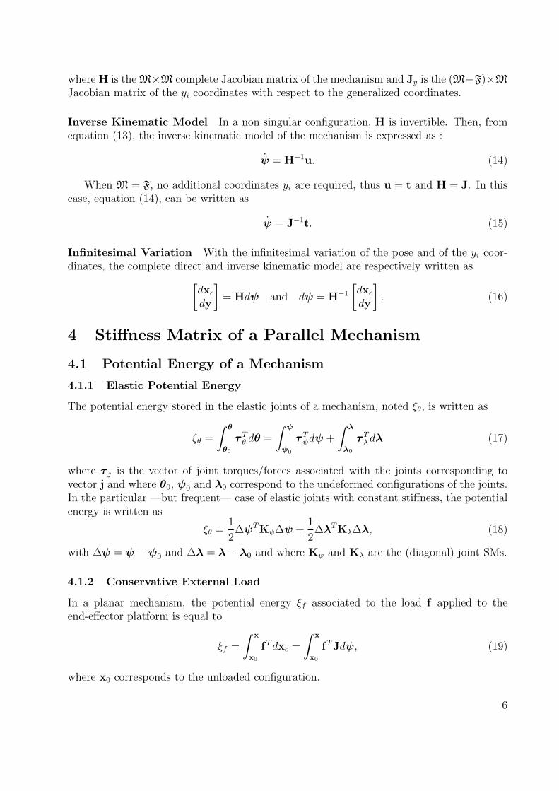
Figure 1: 2-DOF parallel mechanism in an unstable static equilibrium.
maintain stability. For example, one can compute the SM of the 2-DOF mechanism shown inFig.1. When both springs are in tension (ρa > ρa0 and ρb > ρb0), the mechanism is in a stablestatic equilibrium and the SM is positive-definite. When the springs are in compression, themechanism is in an unstable static equilibrium and the SM is non-positive definite since theeigenvalue of the matrix corresponding to the vertical axis is negative. Moreover, it canbe noticed that by choosing θa and ρa as generalized coordinates, the configuration of themechanism shown in Fig.1 is not kinematically singular (i.e., detJ 6= 0 with ψ = [θa, ρa]).
Any other proposed CSM that does not take into account neither the stiffness of thepassive joints nor the effects of the changes of geometry (through matrices KI and KE) willnot allow the description of this phenomenon of instability.
5.3 Other Stiffness Matrices
The CSMs found in the literature can be easily obtained from the matrix presented here,since the latter is more general:
• In the literature, the DOM M is almost always equal to F the degree of freedomof the end-effector platform, thus J−1 exists when the mechanism is not in a singularconfiguration. Therefore, the comparisons in this subsection can be made with eq.(36).
• The matrices for serial mechanisms (Salisbury [21], Chen and Kao [13]) in which thereare no passive joints, i.e., θ = ψ. Thus there are no internal wrenches and KI = 0.
• The matrices when the external wrench f is zero or the Jacobian matrix is constant(Salisbury [21]). Both cases give KE = 0.
• The “infinite” SM of conventional mechanisms that are considered as not sensitive toexternal wrenches. In these cases, the stiffness of the actuators is considered infinite andthat of the passive joints equal to 0, therefore eq.(33) gives KM = diag(∞) and eq.(35)gives KC =∞3×3.
5.4 Use of a Stiffness Matrix
In the literature on the theory of mechanisms, the research papers mainly focus on the F×F
CSM. However, this matrix is not the most useful SM to describe the behaviour of a PM.First, the GSM KM is simpler to obtain and allows a complete description of the mech-
anism, notably when M > F, and of the relation between wrenches and displacements —so
11

can the M×M CSM KU but the latter is more expensive to compute. Note that the conceptof GSM is recent, because before the understanding of the influence of external wrenches onthe stiffness in the 1990’s, KM could not be distinguished from Kψ.
Then, more important than the changes of coordinate basis that, in fine, correspond tothe choice between Cartesian or GSM, the idea of characterizing a mechanism by a stiffnessmatrix is not very relevant. Actually, this choice seems to be due to a mimetism with springsthat are generally characterized by their stiffness. In practice, the computation of the SMis not as useful as that of the compliance matrix that determines the displacement of themechanism due to a variation of the wrenches applied on it. For example, the computation ofthe quasi-static model of a compliant PM [4] requires the determination of the generalizedcompliance matrix, noted CM and equal to K−1
M . The relations between these matricesare written as
CU = HCMHT =
[
CC J CMJTy
JyCMJT Jy CMJTy
]
, (40)
where CC = JCMJT is the F×F Cartesian compliance matrix and CU , the M×M Cartesiancompliance matrix.
5.5 Alternative Formulation
Following the definition of matrices KE and KIG, the calculation of the GSM KM (eq.(33))requires the differentiation of matrices J andG with respect to the generalized coordinates ψ.Yet, in practice an analytical expression of these matrices as functions of ψ is not alwaysknown and thus, their differentiation might not be performed simply. For this reason, anotherformulation of KM has been developed that only requires differentiation with respect to θ.This alternative formulation is detailed in appendix B and is used in the application.
6 Application to a Compliant 3-RPR Mechanism
In this section, the stiffness of a compliant 3-RPR mechanism presented in [18] is studied.This example is relatively simple and the compliant joints are modelled as 1-DOF joints inorder to obtain short and simple formal equations. First, the details of the modelling aregiven, then a comparison between the different SMs proposed in the literature is performedand finally one new possibility offered by the presented SM is used to show the impact ofthe stiffness of the passive joints on the behaviour of this mechanism.
6.1 Modelling of the Mechanism
6.1.1 Geometry of the Mechanism
Geometric Parameters of the Legs Each leg i, indexed from a to c, is defined by thefollowing parameters:• All elastic joints are modelled as 1-DOF joints, thus the DOM of the mechanism is equalto the degree of freedom of the platform: M = F = 3.• The angles associated with the first revolute joints of each leg are noted αi. Their unloaded
12

@@IAa
αa
ρa
βa
���Ab
αb
ρb
βb
-Ac
αc
ρc
βc
x
Figure 2: 3-RPR planar compliant mechanism.
configurations are: αa0 = 0.5404 rad, αb0 = 2.0695 rad and αc0 = −1.8252 rad.• The coordinates of the prismatic joints are noted ρi. Their unloaded configurationsare ρa0 = 583.10mm, ρb0 = 683.22mm and ρc0 = 688.18mm.• The angles associated with the second revolute joints of each leg are noted βi. Their un-loaded configurations are: βa0 = 1.0304 rad, βb0 = −4.6875 rad and βc0 = 1.3016 rad.• The position of the points of the base are Aa = (xa0, ya0) = (−50,−50) cm, Ab = (xb0, yb0)= (50,−50) cm and Ac = (xc0, yc0) = (−50, 76) cm.• The distance between all second revolute joints and the effector’s point of reference: la =lb = lc = l.
Pose of the Platform The pose of the platform, when considered the end-effector ofthe ith leg, is written as
xi =
xiyiφi
=
xi0 + ρicαi + lic(αi + βi)yi0 + ρisαi + lis(αi + βi)
αi + βi
, (41)
where c stands for cos and s for sin. The pose is defined such that x0 = 0 when the externalforces/torques are f = 0.
Geometric Constraints on the Platform The platform of this PM is a rigid body.Hence, the distance between each of the attachment points of the legs on the platform mustremain constant. The position of the attachment point of leg i is noted Ci and is written as
Ci = [xi0 + ρicαi; yi0 + ρisαi]T . (42)
The distance CiCj between 2 points Ci and Cj can be calculated with the following equation,
CiCj =√
(Cj −Ci)T (Cj −Ci)
=√
(xCj − xCi)2 + (yCj − yCi)2 = Lij
(43)
where Lij is the constant distance between Ci and Cj . These constraint equations can thenbe written as
Qij = CiCj2
− L2
ij , ij ∈ {a, b, c}2 , i 6= j. (44)
13

Geometric Constraints and Generalized Coordinates Since there are two indepen-dent kinematic loops in this planar mechanism, 6 constraints have to be satisfied. Thismechanism has 9 joints and thus its number of DOM is 3.
The 3 coordinates ρi are arbitrarily chosen as the generalized coordinates. Thus, thevector of generalized coordinates is written as ψ = [ρa; ρb; ρc]
T and the vector of all the jointcoordinates in the mechanism is written as
θ =
[
ψ
λ
]
=
[
[ρa; ρb; ρc]T
[αa; βa;αb; βb;αc; βc]T
]
, (45)
where λ = [αa; βa;αb; βb;αc; βc]T is the vector of the dependent joint coordinates.
The rigidity of the platform must always be satisfied, i.e., the position (xi, yi) of the endof the 3 legs must be equal2 and the distance between the attachment points must alwaysremain constant. Thus, the constraint function for a kinematic loop is written as :
Kij(θ) =
xi − xjyi − yjQij
= 0. (46)
And the vector of the kinematic constraints for the whole mechanism is defined as
K(θ) =
[
Kab(θ)Kac(θ)
]
. (47)
6.1.2 Kinematics: Infinitesimal Variations
Rigidity of the Platform The differentiation of the square of the distance between theattachment points on the platform with respect to the joint coordinates is calculated as
dQij
dρi= −2cαi(xj0 + ρjcαj − xi0 − ρicαi)
+2sαi(yj0 + ρjsαj − yi0 − ρisαi),
dQij
dαi= 2ρisαi(xj0 + ρjcαj − xi0 − ρicαi)
−2ρicαi(yj0 + ρjsαj − yi0 − ρisαi),
dQij
dβi= 0.
(48)
Kinematic Constraints Matrix S is defined in appendix A.1 and represents the infinitesi-mal kinematic constraints such that Sdθ = 0, ∀dθ. It is equal to dK/dθ. Matrices Sψ and Sλare constructed using the corresponding columns of matrix S, namely
Sλ = [Sα1;Sβ1; . . . ;Sβ3] and Sψ = [Sρ1 ;Sρ2 ;Sρ3] . (49)
2The third component of the pose, representing the orientation of the platform is not used because thisorientation is not a function of ψ, the generalized coordinates.
14

6.1.3 Stiffness Matrix
The formulation presented in equation (68) with the details given in appendix B is used inthis application, namely
KC = J−T[
RT (Kθ +KθE)R+KR
]
J−1. (50)
Matrices G, R, Jλ and J Since all components of matrices Sψ and Sλ are explicitlyknown, a formal expression of matrix G could theoretically be obtained. However, theinversion of the 6 × 6 matrix will lead to a very complex expression, and it is thereforesimpler to compute G numerically, i.e., compute Sψ and Sλ from their formal expressionand then compute the inversion and multiplication as given in appendix A.2.
Matrix Jλ corresponds to the last 6 columns of matrix Jθ and matrix J is obtained byright-multiplying matrix Jθ by matrix R (eq.(11)).
Matrix KθE By definition (eq.64), matrix Kθ
E requires taking the derivative of Jθ. Thisdifferentiation can be preferably performed formally in order to avoid round-off errors dueto a numerical derivation. Moreover, to avoid manipulating a tensor of 3rd order, matrix Kθ
E
is calculated asKθE = Jacobian(JTθ f , θ) (51)
where f = [fx; fy;mφ]T is considered constant.
Matrix KR This matrix is more complicated to compute, because obtaining a formalexpression of R is almost impossible for the 3-RPR mechanism. Therefore, the alternativeformulation of KR detailed in appendix B is used. The algorithm used to implement andcompute matrix KR without introducing numerical errors, is presented below.
• Calculate formal expressions of matrices Sλ and Sψ.
• Calculate a formal expression of matrices Mρ and Mλ, with the constant vector (v =
[v1; · · · ; v6]T ) :
Mρ = Jacobian(STψv, θ),
Mλ = Jacobian(STλv, θ).(52)
• Compute numerically vectors sλ and v :
sλ = Kλ(λ− λ0)− JTλ f and v = S−Tλ sλ. (53)
• Assign the numerical value of the components of v to variables vi to enable the com-putation of Mλ and Mρ.
• Compute numerically R (appendix A.2).
• Finally compute KR :KR = (−Mρ + S−T
ψ S−Tλ Mλ)R. (54)
15
Stiffness Matrix With the above matrices and vectors, the CSM of the 3-RPR mecha-nism can be computed in any non-singular configuration, using the formulation presented ineq.(68).
6.2 Simulation of the Mechanism
In order to illustrate the validity and the accuracy of the proposed SM, a simple applicationis presented below.
The trajectory followed by the 3-RPR mechanism subjected to an external wrench (ap-plied on its end-effector) is computed using the SM. Actually, each increment of the externalwrench multiplied by the SM computed in the local configuration provides an incrementaldisplacement and the combination of all these displacements enables to plot the trajectory.In other words, the trajectory is computed with the following expression, implemented nu-merically:
x← x+K−1
C δf . (55)
On the other hand, the results of the commercial software MSC. Adams are used as referencesto evaluate the accuracy of the computations and indirectly to prove the validity of thepresented SM. In MSC. Adams, the equilibrium and the position of the mechanism arecomputed at each step and therefore there is no drift due to an iterative method. Moreover,by choosing the static simulation option, the dynamical effects are not taken into account,which is consistent with our assumptions. The wrench applied on the reference point of theplatform is
f(t) = [f0 sin(2πt); f0 sin(4πt); 0]T , f0 = 100N. (56)
6.2.1 Comparison with Other Formulations
In this subsection, we consider a mechanism in which the stiffness of the actuators are finitebut the stiffness of the passive joints is equal to zero.
With this simulation, we can compare (a) the accuracy of the SM presented by Salis-bury [21], (b) the accuracy of the SM presented by Chen and Kao [13] and (c) the accuracyof the proposed SM. The SM for PMs presented in this paper is noted PM (c). Matrices (c)and (b) represents the conservative congruence transformation (CCT).
To make the comparison between all these matrices, matrix (c) is computed with thevalue of stiffness of the passive joints equal to zero (Kλ = 0). Thus, formulations (b)and (c) become equivalent, but since their implementation are different, mainly becauseof the alternative formulation used here, their computation can provide slightly differentresults. The three expressions of KC are written as
(a) Salisbury : KC = J−Tρ KρJ
−1
ρ
(b) Chen : KC = J−Tρ (Kρ +K
ρE)J
−1
ρ
(c) PM : KC = J−T (Kψ +KI +KE)J−1
(57)
where Jρ is the Jacobian matrix usually used for the 3-RPR mechanism, Kρ is the 3 × 3diagonal matrix representing the stiffness of the actuators ρi and K
ρE corresponds to the
matrix (−KG) defined in [13]. In cases (a) and (c), the coordinates of the passive joints αi
16

−0.06 −0.04 −0.02 0 0.02 0.04 0.06−0.04
−0.03
−0.02
−0.01
0
0.01
0.02
0.03
0.04
(a) Salisbury
(b) Kao
(c) CPM
Adams
y
x
Figure 3: Trajectory (x, y) described by the mechanism subjected to f(t).
0 50 100 150 200 250 300−1
−0.5
0
0.5
1
1.5
2
2.5
3x 10
−3
(a) Salisbury
(b) Kao
(c) CPM
Adams
∆y
t
Figure 4: Discrepancy in x-coordinate of the pose of the mechanism subjected to f(t).
and βi do not appear. The time of simulation t varies from 0 s to 1 s in 250 iterations, suchthat δt = 1/250 s (4ms). The increment of external wrench is δf = f ′(t)δt. And the stiffnessvalues of the joints used in this section are kα = kβ = 0N.rad−1 and kρ = 2000N.mm−1.
Results Figure 3 shows the trajectory described by the mechanism, computed with thesoftware MSC. Adams and with the four matrices. It can be noticed that the results obtainedwith matrix (a) does not correspond to the trajectory computed with MSC. Adams, whileresults of the CCT matrices (b) and (c) are accurate. Since the results are very close to eachother, they are presented in another form in Figs. 4, 5 and 6. The latter graphs show thedifference in the 3 components (x,y,φ) of the pose x, between the reference from MSC. Adamsand the computation with each matrix.
Some important points can be noted on the graphs:• The discrepancy between the results obtained with MSC. Adams and with the CCT matri-ces increases uniformly as the simulation proceeds. This effect is a drift due to the iterativecomputation. In a real use of these matrices, the variables are updated by a measurementon the robot at each step, thus this drift should disappear.• On the contrary, the discrepancy between the results obtained with MSC. Adams andSalisbury’s matrix is clearly a function of the external loads. The larger these loads are, thelarger the error in the stiffness computation will be. The drift due to the iterative computa-
17

0 50 100 150 200 250 300−3
−2.5
−2
−1.5
−1
−0.5
0
0.5x 10
−3
(a) Salisbury
(b) Kao
(c) CPM
Adams
∆y
t
Figure 5: Discrepancy in y-coordinate of the pose of the mechanism subjected to f(t).
0 50 100 150 200 250 300−2
0
2
4
6
8
10
12x 10
−3
(a) Salisbury
(b) Kao
(c) CPM
Adams
∆φ
t
Figure 6: Discrepancy in φ-coordinate of the pose of the mechanism subjected to f(t).
tion also exists but it is secondary compared to the effect of loads. We can however observethat the error due to the load seems to be compensated for since the error decreases whenthe load decreases.• As shown in Fig. 3, the simulation with the CCT matrices are much more accurate thanwith Salisbury’s matrix. The range of deviation for the CCT matrices after 250 iterationsis 0, 5µm in position and 2.10−3 rad in orientation, while the maximal deviation for Salis-bury’s matrix is 3µm in position and 1, 2.10−2 rad in orientation.• A small difference between matrices (b) and (c) can be noticed at the end of the simulation(notably in Fig. 5 and Fig. 6). These differences are only due to the numerical computations.
Conclusion This simulation confirms the validity and the equivalence of both CCT for-mulations. It also shows their accuracy. On the other hand, this simulation proves theinvalidity of Salisbury’s matrix. Indeed, if the latter matrix can seem acceptable for verysmall external wrenches such as vibrations, the error grows quickly with the loads.
6.2.2 Impact of the Passive Joints
The main novelty of the SM proposed in this paper is the possibility to take into account thestiffness of the passive joints. Figure 7 illustrates this new possibility and shows the trajectory
18

−0.06 −0.04 −0.02 0 0.02 0.04 0.06−0.03
−0.02
−0.01
0
0.01
0.02
0.03
0.04
0 N/rad
10 N/rad
100 N/rad
y
x
Figure 7: Trajectory (x, y) described by different mechanisms subjected to f(t).
performed by the mechanism when it is subjected to the external wrench f(t) defined ineq.(56). This trajectory is computed with passive joints having different stiffness kαi
and kβi,namely: 0N.rad−1, 10N.rad−1 and 100N.rad−1. Note that the trajectories calculated withMSC. Adams are not represented in figure 7 because they coincide exactly with those of ourmodel. The discrepancy cannot be observed at this scale.
As expected, it can be observed that stiffer passive joints give a stiffer mechanism anddecrease the amplitude of the displacement due to external wrenches. The shape of thedisplacement is also affected. The curve drawn with crosses represents the trajectory of amechanism in which the stiffness of the passive joint is only 20 times smaller than that of theactuators, but even in this extreme and almost unrealistic case, the trajectory is computedwith a very good accuracy.
The important point illustrated by this application is the possibility to accurately deter-mine the behaviour of a mechanism subjected to external loads. Indeed, the stiffness of thepassive joints can be regarded as an advantage or as a disadvantage in the context of controlof a manipulator since it makes the manipulator less sensitive to external perturbations butrequires more powerful actuators. However, if high precision is required, with the new SMthat enables to compute accurately their behaviour, compliant joints with zero mechanicalclearance offer only advantages. In other words, with the knowledge of the SM, the precisionof a mechanism becomes independent from its stiffness.
7 Conclusion
The proposed formulation of the stiffness matrix is clear and meaningful. The presentedCartesian stiffness matrix is a generalization of the already existing matrices published inthe literature, since it can take into account non-zero external loads, non-constant Jacobianmatrices, stiff passive joints and additional compliances, these two latter points being itsmain novelty.
Moreover, the results predicted with this stiffness matrix are very accurate and the pro-posed SM enables a very accurate control of parallel manipulators built with elastic joints.
19

Acknowledgements
The authors would like to acknowledge the financial support of the Natural Sciences andEngineering Research Council of Canada (NSERC) as well as the Canada Research Chair(CRC) Program.
References
[1] Kovecses, J. and Angeles, J., 2007, “The Stiffness Matrix in Elastically ArticulatedRigid-Body Systems,” Multibody System Dynamics, 18(2), pp. 169–184.
[2] Howell, L., 2001, Compliant Mechanisms, Wiley-Interscience.
[3] Su, H.-J., 2009, “A Pseudorigid-Body 3R Model for Determining Large Deflection ofCantilever Beams Subject to Tip Loads,” Journal of Mechanisms and Robotics, 1(2),021008.
[4] Quennouelle, C. and Gosselin, C., 2009, “A Quasi-Static Model for Planar CompliantParallel Mechanisms,” Journal of Mechanisms and Robotics, 1(2), 021012.
[5] Li, Y., Chen, S., and Kao, I., 2002, “Stiffness Control and Transformation for RoboticSystems with Coordinate and Non-Coordinate Bases,” IEEE International Conferenceon Robotics and Automation, vol. 1.
[6] Chen, S., 2003, “The 6×6 Stiffness Formulation and Transformation of Serial Manipula-tors via the CCT Theory,” IEEE International Conference on Robotics and Automation,vol. 3.
[7] Howard, W., Zefran, M., and Kumar, V., 1998, “On the 6×6 Cartesian Stiffness Matrixfor Three-Dimensional Motions,” Mechanism and Machine Theory, 33(4), pp. 389–408.
[8] Zefran, M. and Kumar, V., 2002, “A Geometrical Approach to the Study of the Carte-sian Stiffness Matrix,” Journal of Mechanical Design, 124(1), pp. 30–38.
[9] Svinin, M., Hosoe, S., and Uchiyama, M., 2001, “On the Stiffness and Stability ofGough-Stewart Platforms,” IEEE International Conference on Robotics and Automa-tion, vol. 4.
[10] Ciblak, N. and Lipkin, H., 1994, “Asymmetric Cartesian Stiffness for the Modeling ofCompliant Robotic Systems,” 23rd Biennial Mechanical Conference, Design Engineer-ing Division, vol. 72.
[11] Zefran, M. and Kumar, V., 1997, “Affine Connections for the Cartesian Stiffness Ma-trix,” IEEE International Conference on Robotics and Automation, vol. 2.
[12] Ciblak, N. and Lipkin, H., 1999, “Synthesis of Cartesian Stiffness for Robotic Applica-tions,” IEEE International Conference on Robotics and Automation, vol. 3.
20

[13] Chen, S. and Kao, I., 2000, “Conservative Congruence Transformation for Joint andCartesian Stiffness Matrices of Robotic Hands and Fingers,” The International Journalof Robotics Research, 19(9), pp. 835–847.
[14] Huang, C., Hung, W., and Kao, I., 2002, “New Conservative Stiffness Mapping for theStewart-Gough Platform,” IEEE International Conference on Robotics and Automation,pp. 823–828.
[15] Li, Y. and Kao, I., 2001, “On the Stiffness Control and Congruence TransformationUsing the Conservative Congruence Transformation (CCT),” IEEE International Con-ference on Robotics and Automation, pp. 823–828.
[16] Kao, I. and Ngo, C., 1999, “Properties of the Grasp Stiffness Matrix and ConservativeControl Strategies,” The International Journal of Robotics Research, 18(2), pp. 159–167.
[17] Chen, S., 2005, “The Spatial Conservative Congruence Transformation for Manipula-tor Stiffness Modeling with Coordinate and Noncoordinate Bases,” Journal of RoboticSystems, 22(1), pp. 31–44.
[18] Su, H.-J. and Mc Carthy, J., 2006, “A Polynomial Homotopy Formulation of the In-verse Static Analysis of Planar Compliant Mechanisms,” ASME Journal of MechanicalDesign, 128(4), pp. 776–786.
[19] Carricato, M., Duffy, J., and Parenti-Castelli, V., 2002, “Catastrophe Analysis of aPlanar System with Flexural Pivots,” Mechanism and Machine Theory, 37(7), pp. 693–716.
[20] Carricato, M., Duffy, J., and Parenti-Castelli, V., 2000, “The Stiffness Matrix and theHessian Matrix of the Total Potential Energy in Mechanisms,” Publication no. 111 ofDIEM, Dept. of Mechanical Engineering of the University of Bologna, Italy, pp. 1–17.
[21] Salisbury, J., 1980, “Active Stiffness Control of a Manipulator in Cartesian Coordi-nates,” 19th IEEE Conference on Decision and Control, pp. 87–97.
[22] Gosselin, C., 1990, “Stiffness Mapping for Parallel Manipulators,” IEEE Transactionson Robotics and Automation, 6(3), pp. 377–382.
[23] Merlet, J., 2006, Parallel Robots, Kluwer Academic Publisher.
[24] Griffis, M. and Duffy, J., 1993, “Global Stiffness Modeling of a Class of Simple CompliantCouplings,” Mechanism and machine theory, 28(2), pp. 207–224.
[25] Zhang, D., 2000, Kinetostatic Analysis and Optimization of Parallel and Hybrid Archi-tectures for Machine Tools, Ph.D. thesis, Universite Laval, Quebec, QC, Canada.
[26] Zhang, D. and Gosselin, C., 2002, “Kinetostatic Modeling of Parallel Mechanisms witha Passive Constraining Leg and Revolute Actuators,” Mechanism and Machine Theory,37(6), pp. 599–617.
21

[27] Cho, W., Tesar, D., and Freeman, R., 1989, “The Dynamic and Stiffness Modeling ofGeneral Robotic Manipulator Systems with Antagonistic Actuation,” IEEE Interna-tional Conference on Robotics and Automation, pp. 1380–1387.
[28] Yi, B., Chung, G., Na, H., Kim, W., and Suh, I., 2003, “Design and Experiment ofa 3-DOF Parallel Micromechanism Utilizing Flexure Hinges,” IEEE Transactions onRobotics and Automation, 19(4), pp. 604–612.
[29] Quennouelle, C., 2009, Modelisation geometrico-statique des mecanismes paralleles com-pliants, Ph.D. thesis, Universite Laval, Quebec, QC, Canada.
[30] Angeles, J., 2003, Fundamentals of Robotic Mechanical Systems: Theory, Methods, andAlgorithms, Springer.
[31] Chen, S. and Kao, I., 2000, “Geometrical Method for Modeling of Asymmetric 6×6Cartesian Stiffness Matrix,” IEEE/RSJ International Conference on Intelligent Robotsand Systems, vol. 2.
A Matrices of Constraints
A.1 Matrices S, Sλ and Sψ
From the geometric constraints (eq.(4)), the kinematic constraints of a PM can also bewritten as
dK(θ) =dK(θ)
dθdθ = Sdθ = 0, (58)
where matrix is S is defined as the derivative of K with respect to θ. Making the distinctionbetween the generalized and the dependent coordinates, one can write
Sdθ = [Sψ;Sλ]
[
dψdλ
]
= Sψdψ + Sλdλ = 0, (59)
where Sψ is the C×M matrix composed of the M columns of S corresponding to ψ and Sλis the C× C matrix composed of the C columns of S corresponding to λ.
A.2 Matrices G and R
By definition, the C coordinates λi are the solutions of the C geometrical constraints K
for a set ψ, so Sλ = dK/dλ is a matrix of full rank and therefore is always invertible.Equation (59) is equivalent to
dλ = −S−1
λ Sψdψ. (60)
Thus, matrices G and R are expressed as
G = −S−1
λ Sψ and R =
[
1M
−S−1
λ Sψ
]
. (61)
22

B Implementation of the Stiffness Matrix
B.1 Alternative Formulation of KC
B.1.1 Matrix KE
In some PMs, a formal expression of J as a function of ψ can be difficult to obtain whereas Jθis easy to formulate as a function of coordinates θi. And G and R are defined as functionof θ. Therefore, it is generally more interesting to calculate d(·)/dθ instead of d(·)/dψ.Using equation (11), the definition of KE (eq.(29)) is equivalent to
KE =−dJ
dψ
T
f = −d(JθR)
dψ
T
f
= −RT (dJθdθ
T
f)dθ
dψ−dR
dψ
T
JTθ f
(62)
In this equation, matrix (−dJθ/dθ)T f is noted Kθ
E. In this matrix, the kinematic constraintsare not taken into account, each leg is considered as an independent mechanism. Hence,since RT =
[
1;GT]
, the last term of eq.(62) is noted KEG and can be calculated as
KEG = −dR
dψ
T
JTθ f = −d1
dψ
T
JTψf −dG
dψ
T
JTλ f
= −
[
dG
dθ
T
JTλ f
]
R.
(63)
where Jλ = dxc/dλ contains the columns of Jθ corresponding to coordinates λi. Thus eq.(62)can be written as
KE = RTKθER+KEG. (64)
B.1.2 Matrix KI
A matrix KR that represents the effects of the change of the constraints GT is defined by
KR = KIG +KEG =dG
dψ
T
τ λ −dG
dψ
T
JTλ f . (65)
Thus, with the same operations as in section (B.1.1), KR is calculated as
KR =
[
dG
dθ
T
(τ λ − JTλ f)
]
R =
[
dG
dθ
T
sλ
]
R. (66)
where sλ represents the sum of the forces/torques applied on the constrained joints.
B.1.3 Cartesian Stiffness Matrix
Using the above matrices, KC can be written as
KC = J−T(
Kψ +GTKλG+KR +RTKθER
)
J−1. (67)
This latter equation being equivalent to
KC = J−T[
RT (Kθ +KθE)R+KR
]
J−1 (68)
23

B.2 Computation of Matrix KR
Matrix KR results from the differentiation of matrix G. But since a formal expression of Gmight be too complex to be handled in closed form due to the inversion of the (C × C)matrix Sλ, an alternative method to calculate it can be used. Moreover, the derivative of amatrix with respect to a vector gives a tensor of 3rd order, and this type of mathematicalobject and all its associated functions are usually not developed in most current softwarepackages. For the above reasons, a detailed formulation of KR is presented below. Thisformulation is easier to implement and it enables the computation of KR without introducingnumerical inaccuracies.
To avoid taking the derivative of matrix S with respect to vector θ—which gives a tensorof 3rd order— the vector GT sλ is first calculated
GT sλ = −S−1
λ STψsλ. (69)
Then, the Jacobian matrix of GT sλ with respect to θ can be calculated, considering sλ as aconstant vector (noted sλ)
dGT
dθsλ =
d(GT sλ)
dθ=d(−STψS
−Tλ )
dθsλ. (70)
Equation (70) is equivalent to :
dGT
dθsλ = −
dSTψdθ
S−Tλ sλ − STψ
dS−Tλ
dθsλ. (71)
Since calculating a formal expression of S−1
λ might be too complex and since a formal deriva-tive is desired to avoid any round-off errors in the computation ofKS, the following equivalentformulation of S−T
λ is used. In this equation, the inversion can be computed numerically butthe derivative can be obtained formally.
dS−Tλ
dθ= −S−T
λ
dSTλdθ
S−Tλ . (72)
Thus, equation (71) is equivalent to
dGT
dθs = −
dSTψdθ
S−Tλ sλ + STψS
−Tλ
dSTλdθ
S−Tλ sλ. (73)
Here again, the derivative of a matrix with respect to a vector is required. To avoid such aderivative, the following vectors are introduced :
v = S−Tλ sλ
mψ = STψS−Tλ sλ = STψv
mλ = STλS−Tλ sλ = STλv
(74)
For practical purposes, the vectors mψ and mλ are formally calculated with a vector of
constant components (v = [v1, · · · , vC]T ), then the formal derivatives are calculated. Finally,
24

the numerically computed components of v are assigned to variables vi to obtain matricesMψ
and Mλ.
dSTψdθ
S−Tλ sλ =
dmψ
dθ= Mψ
dSTλdθ
S−Tλ sλ =
dmλ
dθ= Mλ
(75)
An alternative formulation of matrix KR defined in eq.(66) can then be written as
KR =
[
−dSTψdθ
S−Tλ sλ + STψS
−Tλ
dSTλdθ
S−Tλ sλ
]
R. (76)
25