a generalized numerical framework of imprecise probability...

A generalized numerical framework of impreciseprobability to propagate epistemic uncertainty

Marco de Angelis,E. Patelli, M. Beer

E: [email protected]: www.liv.ac.uk/risk-and-uncertaintyT: +44 01517945481

M. de Angelis, et al. 26th May 2014 1 / 30

Outline

1 Introduction

2 Uncertainty propagationImprecise failure probabilityLine sampling estimation

3 ExamplesExplicit functionLarge scale finite element model

4 Conclusions


Introduction

Problem statement

Computer modelReliability assessmentDecision making


Introduction

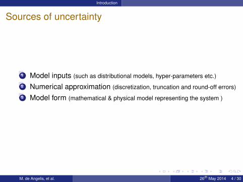
Sources of uncertainty

1 Model inputs (such as distributional models, hyper-parameters etc.)

2 Numerical approximation (discretization, truncation and round-off errors)

3 Model form (mathematical & physical model representing the system )


Introduction

Uncertainty framework

VerificationNumerical approximation

Discretization errorsRound-off errors

Uncertainty propagationpropagation of input uncertainties through the modelprocessing of output uncertainties

Validationcheck the model against experimental data

Decisionidentify the worst case scenariodecide whether worst case is acceptable


Introduction

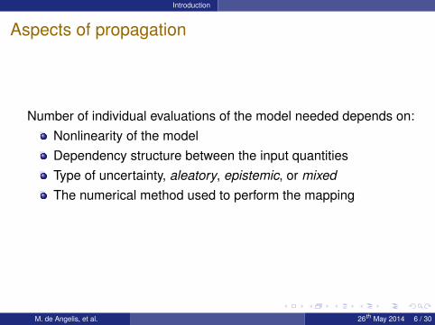
Aspects of propagation

Number of individual evaluations of the model needed depends on:Nonlinearity of the modelDependency structure between the input quantitiesType of uncertainty, aleatory, epistemic, or mixedThe numerical method used to perform the mapping


Introduction

Parametric approachStandard approach

1

2

j

n

p1

p3

pj

pm-1

pm

p2

p4

f1(.) f2(.) f3(.) RQ

Monte Carlo Simulation

RQ

Simulated CDFGlobal Optimization

i

a1i

a2i

aji

a2i

Search feasible domain B

i

θ

θ

θ

θ

pF = 1N

i=1

N

I (RQ<0)i

EPR=1N

i=1

N

RQi


Introduction

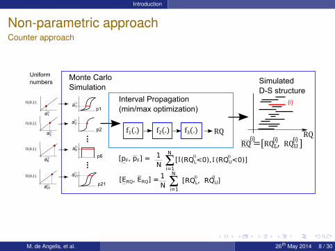
Non-parametric approachCounter approach

p1

p2

p6

p21

U(0,1)

a1i

a1i

U(0,1)

a6i

a6i

U(0,1)

a2i

U(0,1)

a21i

a2i

a21i

Interval Propagation(min/max optimization)

RQ

i

RQ=[RQL,RQU]i i i

SimulatedD-S structure

f1(.) f2(.) f3(.) RQ


Uniform numbers

1N

i=1

N

I(RQL<0), (RQU<0)]i[pF, pF] = [ I

i

1N

i=1

N

RQL, RQU]i[ERQ, ERQ] = [

i


Introduction

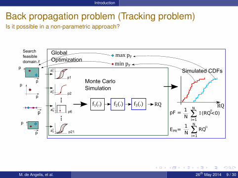
Back propagation problem (Tracking problem)Is it possible in a non-parametric approach?

p1

p2

p6

p21

p

p

p

p

p

p

p


RQ

Simulated CDFs

Global Optimization

a1i

a2i

a6i

a2i

Search feasible domain B minpF

maxpF

pF = 1N

i=1

N

I (RQ<0)i

EPR=1N

i=1

N

RQi

f1(.) f2(.) f3(.) RQ


Introduction

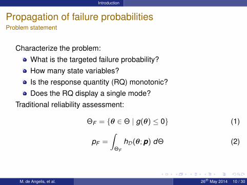
Propagation of failure probabilitiesProblem statement

Characterize the problem:What is the targeted failure probability?How many state variables?Is the response quantity (RQ) monotonic?Does the RQ display a single mode?


Introduction

Propagation of failure probabilitiesProblem statement

Characterize the problem:What is the targeted failure probability?How many state variables?Is the response quantity (RQ) monotonic?Does the RQ display a single mode?

Traditional reliability assessment:

ΘF = θ ∈ Θ | g(θ) ≤ 0 (1)

pF =

∫ΘF

hD(θ; p) dΘ (2)


Uncertainty propagation

Outline

1 Introduction



4 Conclusions


Uncertainty propagation Imprecise failure probability

Generalized numerical framework of uncertainties

A bounded set B is defined by a vector of intervals x i , i = 1, ...,nxand a dependence function Φ(x)

B =×nxi=1[Φ(xi), Φ(xi)] (3)

A credal set C is the set of distribution functions

C = hD (ξ; p) | p ∈ Bp , Bp =×npi [pi , pi ] (4)



Generalized numerical framework of uncertaintiesA bounded set B is defined by a vector of intervals x i , i = 1, ...,nxand a dependence function Φ(x)

B =×nxi=1[Φ(xi), Φ(xi)] (3)

A credal set C is the set of distribution functions

C = hD (ξ; p) | p ∈ Bp , Bp =×npi [pi , pi ] (4)

Redefinition of failure domain:

ΘF = ΩF × XF (5)

where,ΩF (x) = ξ ∈ Rnξ | g(ξ,x) ≤ 0 , (6)

XF (ξ) = x ∈ Rnx | g(ξ,x) ≤ 0 . (7)



Failure probabilityLower and upper bounds

Lower and upper bounds of failure probability are

pF

(C,Bx ) = infx∈Bx p∈Bp

∫ΩF (x)

hD(ξ; p) dΩ; (8)

pF (C,Bx ) = supx∈Bx p∈Bp

∫ΩF (x)

hD(ξ; p) dΩ. (9)



Failure probabilityConjugate relationship

When the uncertainty setM is restricted to C only, i.e. M = C, theprobability function h that yields the lower bound p

Fsatisfies∫

ΩF

hD(ξ) dΩ +

∫ΩS

hD(ξ) dΩ = 1, (10)

where, ΩF ∪ ΩS = Ω. Then, Eq. (9) establishes a conjugate (dual)relationship

p(ΩS) = 1− p(ΩF ), (11)

with p(ΩS) =∫

ΩShD(ξ) dΩ and p(ΩF ) =

∫ΩF

hD(ξ) dΩ.


Uncertainty propagation Line sampling estimation

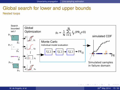
Global search for lower and upper boundsNested loops

1

2

i

n

f(.) f(.) PR

Monte Carlo Individual model evaluation

0 PR

simulated CDF

Global Optimization

i

a1i

a2i

a6i

a2i

Search bounded set B

if(.)1 2 3

p1

p2p3

p4

pi

pm-1

pm

pF =1N

I (PR <0)ii=1

N

F

Simulated samples in failure domain



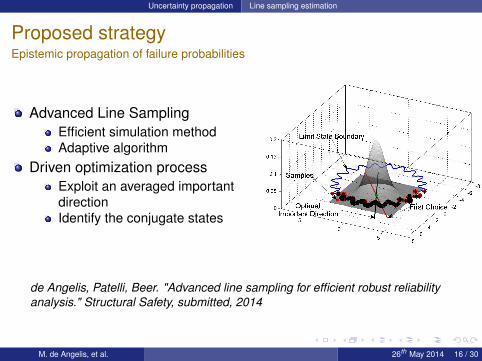
Proposed strategyEpistemic propagation of failure probabilities

Advanced Line SamplingEfficient simulation methodAdaptive algorithm

Driven optimization processExploit an averaged importantdirectionIdentify the conjugate states

de Angelis, Patelli, Beer. "Advanced line sampling for efficient robust reliabilityanalysis." Structural Safety, submitted, 2014



Line Sampling

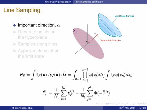
Important direction, αGenerate points onthe hyperplaneSamples along linesApproximate point onthe limit state

Limit State Surface

Sta

Important Direction

PF =

∫IF (x) hN (x) dx =

∫n−1

n−1∏j=1

φ(xj)dxj

∫IFφ(xn)dxn

PF =1

NL

NL∑j=1

p(j)F =

1NL

NL∑j=1

Φ(−¯(j))



Line Sampling


Sta

PF =


∫n−1

n−1∏j=1

φ(xj)dxj

∫IFφ(xn)dxn

PF =1

NL

NL∑j=1

p(j)F =

1NL

NL∑j=1

Φ(−¯(j))



Line Sampling


Line sample

Line

Xt(j) + l(j) a

Xt(j)

l(j)

Sta

PF =


∫n−1

n−1∏j=1

φ(xj)dxj

∫IFφ(xn)dxn

PF =1

NL

NL∑j=1

p(j)F =

1NL

NL∑j=1

Φ(−¯(j))



Line Sampling


Intersectionw/ LSF

Xt(j) + l a

Sta

PF =


∫n−1

n−1∏j=1

φ(xj)dxj

∫IFφ(xn)dxn

PF =1

NL

NL∑j=1

p(j)F =

1NL

NL∑j=1

Φ(−¯(j))



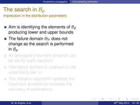
The search in BpImprecision in the distribution parameters

Aim is identifying the elements of Bpproducing lower and upper boundsThe failure domain ΘF does notchange as the search is performedin Bp

An averaged important direction canbe set for each iterationThe failure domain is invariant to theuncertainty setMThe adaptive algorithm updates theimportant direction to increase theaccuracy of estimations






1

- 3

- 2

- 1

Physical Space

xi

xj

Standard Normal Spaceuj

ui






1 2

- 3

- 2

- 1Standard Normal Spaceuj

ui

xi

xj Physical Space






1 2

- 3

- 2

- 1

uj

ui

xi

xj Physical Space

Standard Normal Space



The search in BxImprecision in the structural parameters

Recall the definition of failure domain from Eq. (4):

ΩF (x) = ξ ∈ Rnξ | g(ξ,x) ≤ 0 ,

Intervals make the failure domain no longer invariant to theuncertainty setM,For the sake of searching in Bx , assume the intervals areimprecise Gaussian random variables

x → η ∈ Cx =

hN (η;µx ,σx ) | µx = x , σx ∈ [0,x r ], (12)

The uncertainty set is now the credal setM′ = C ∪ Cx



The search in BxImprecision in the structural parameters

The search inM′ allows to identify the conjugate states

µ∗ = arg minM′

pF , µ∗ = arg maxM′

pF (13)

To these states it is associated the corresponding argumentminimum and maximum to be held within the intervals

(µx∗, µ∗x )→ (x∗, x∗) (14)

As the argument optima (x∗, x∗) are identified in Bx , just twomore reliability analyses are needed to estimate lower andupper failure probabilities.


Examples Explicit function

Outline

1 Introduction



4 Conclusions



Linear performance function with noisecase (a): description

g(ξ,x) = −500 + ξ1 + 2ξ2 + 2ξ3 + ξ4 − 5x1 − 5x2 +

+0.0014∑

i=1

sin(100ξi) + 0.0012∑

j=1

sin(100xj);

SV Symbol Uncert. type Mean/Interval Stand. dev.

1 ξ1 LN(µ1, σ1) µ1 = [110, 125] σ1 = [10, 14]

2 ξ2 LN(µ2, σ2) µ2 = [115, 130] σ2 = [10, 14]

3 ξ3 LN(µ3, σ3) µ3 = [115, 130] σ3 = [10, 14]

4 ξ4 LN(µ4, σ4) µ4 = [115, 130] σ4 = [10, 14]

5 x1 Interval x1 x1 = [45, 52] -6 x2 Interval x2 x2 = [35, 43] -



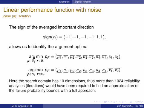
Linear performance function with noisecase (a): solution

The sign of the averaged important direction

sign(α) = (−1,−1,−1,−1,1,1),

allows us to identify the argument optima

arg minp∈Bξ x∈Bx

pF = (µ1, σ1, µ2, σ2, µ3, σ3, µ4, σ4, x1, x2),

arg maxp∈Bξ x∈Bx

pF = (µ1, σ1, µ2, σ2, µ3, σ3, µ4, σ4, x1, x2).

Here the search domain has 10 dimensions, thus more than 1024 reliabilityanalyses (iterations) would have been required to find an approximation ofthe failure probability bounds with a full approach.



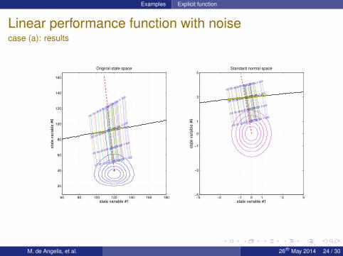
Linear performance function with noisecase (a): results

state variable #1

sta

te v

ariable

#6

Original state space

60 80 100 120 140 160 180

20

40

60

80

100

120

140

160

state variable #1

sta

te v

ara

ible

#6

Standard normal space

−5 −3 −1 0 1 3 5−5

−3

−1

0

1

3

5



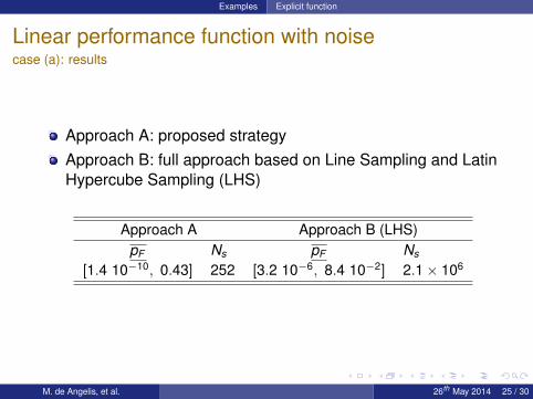
Linear performance function with noisecase (a): results

Approach A: proposed strategyApproach B: full approach based on Line Sampling and LatinHypercube Sampling (LHS)

Approach A Approach B (LHS)pF Ns pF Ns

[1.4 10−10, 0.43] 252 [3.2 10−6, 8.4 10−2] 2.1× 106


Examples Large scale finite element model

Six-level buildingimprecision in distribution parameters

244 State Variables, 8200 elements,66300 degrees of freedomColumns’ depth and breadth are theinterval [0.36, 0.44]mPerformance function:g(θ) = |σI(θ)− σIII(θ)| /2− σy ,

Investigate sensitivity of failureprobabilities against imprecisionIdentify the worst case scenario

Robust realibility analysis





Investigate sensitivity of failureprobabilities against imprecisionIdentify the worst case scenario


3 3.2 3.4 3.6 3.8 4 4.2 4.4 4.6 4.8

−1.5

−1

−0.5

0

0.5

1

x 107

distance fromhyperplane

performance

values





Objectives:Investigate sensitivity of failureprobabilities against imprecisionIdentify the worst case scenario


3 3.2 3.4 3.6 3.8 4 4.2 4.4 4.6 4.8

−1.5

−1

−0.5

0

0.5

1

x 107

distance fromhyperplane

performance

values



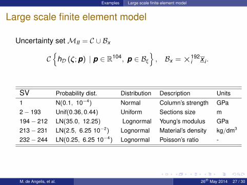
Large scale finite element model

Uncertainty setMII = C ∪ Bx

C

hD (ζ; p) | p ∈ R104, p ∈ Bξ, Bx =×192

i x i .

SV Probability dist. Distribution Description Units

1 N(0.1, 10−4) Normal Column’s strength GPa2 − 193 Unif(0.36, 0.44) Uniform Sections size m194 − 212 LN(35.0, 12.25) Lognormal Young’s modulus GPa213 − 231 LN(2.5, 6.25 10−2) Lognormal Material’s density kg/dm3

232 − 244 LN(0.25, 6.25 10−4) Lognormal Poisson’s ratio -



Large scale finite element model

Uncertainty setMII = C ∪ Bx

C

hD (ζ; p) | p ∈ R104, p ∈ Bξ, Bx =×192

i x i .

SV Uncertainties type p = pc [1 − ε, 1 + ε], x = [x , x ]

1 distribution N(µ, σ2) µc = 0.1 σc = 0.012 − 193 interval x x = 0.36 x = 0.44194 − 212 distribution LN(m, v) mc = 35 vc = 12.25213 − 231 distribution LN(m, v) mc = 2.5 vc = 6.25 10−2

232 − 244 distribution LN(m, v) mc = 0.25 vc = 6.25 10−4



Large scale finite element modelResults

Lower Bound Upper Boundε p

FCoV pF CoV Ns

0.000 4.70 10−7 10.2 10−2 6.73 10−3 11.5 10−2 2590.010 2.28 10−7 13.4 10−2 9.71 10−3 12.2 10−2 2470.015 1.10 10−7 10.3 10−2 1.11 10−2 7.6 10−2 2550.020 5.19 10−8 13.1 10−2 2.08 10−2 14.6 10−2 2550.025 2.51 10−8 9.97 10−2 2.72 10−2 15.3 10−2 2490.030 1.40 10−8 9.94 10−2 3.21 10−2 6.5 10−2 254



Large scale finite element modelResults

0

0.1

0.2

0.3

0.4

0.5

0.6

0.7

0.8

0.9

1

mem

bers

hip

pc(1- ) pc(1+ )3 3pc

3=0.03

3=0.075

3=0.05

3=0.025

3=0.01

3=0

10−8

10−7

10−6

10−5

10−4

10−3

10−2

10−1

0

0.1

0.2

0.3

0.4

0.5

0.6

0.7

0.8

0.9

1

mem

bers

hip

pF

(a) (b)


Conclusions

Outline

1 Introduction



4 Conclusions


Conclusions

Final remarksA strategy to propagate epistemic uncertainty with the failureprobability was proposedBounded and Credal sets are formulated as a sound way toaccount for epistemic uncertainty in a parametric senseWith the proposed numerical strategy, uncertainty propagation’sefficiency can be significantly increasedWhen the underlying model displays monotonic, time of theanalysis is comparable to a single Monte CarloThe strategy is generally applicable so far as the model displaysa single failure modeThe solution strategy is integrated in the general purposesoftware Open Cossan


a generalized numerical framework of imprecise probability...

Documents