a generic evaluation of a categorical compositional ... · a generic evaluation of a categorical...
TRANSCRIPT
A Generic Evaluation of a CategoricalCompositional-distributional Model of
Meaning
University of OxfordMSc Computer Science
Jiannan Zhang
St Cross College
Candidate Number: 409265
Supervisors: Bob Coecke, Dimitri Kartsaklis
August 31, 2014
Contents
Acknowledgements 3
Abstract 5
1 Introduction 6
2 Background 92.1 Formal semantics . . . . . . . . . . . . . . . . . . . . . . . . . 92.2 Distributional semantics . . . . . . . . . . . . . . . . . . . . . 112.3 Compositionality in distributional models of meaning . . . . . 12
2.3.1 Additive models . . . . . . . . . . . . . . . . . . . . . . 122.3.2 Multiplicative models . . . . . . . . . . . . . . . . . . . 132.3.3 Sentence living in tensor space . . . . . . . . . . . . . . 132.3.4 Other models . . . . . . . . . . . . . . . . . . . . . . . 14
2.4 A categorical framework of meaning . . . . . . . . . . . . . . . 152.4.1 Category . . . . . . . . . . . . . . . . . . . . . . . . . . 152.4.2 Monoidal category . . . . . . . . . . . . . . . . . . . . 162.4.3 Compact closed categories . . . . . . . . . . . . . . . . 172.4.4 Pregroups grammar and FVect as compact closed cate-
gories . . . . . . . . . . . . . . . . . . . . . . . . . . . 182.4.5 A passage from syntax to semantics . . . . . . . . . . . 202.4.6 Frobenius Algebra . . . . . . . . . . . . . . . . . . . . 21
2.5 Progress of building practical models and evaluation of the cat-egorical model . . . . . . . . . . . . . . . . . . . . . . . . . . . 22
3 Methodology 233.1 Semantic word spaces for the categorical model . . . . . . . . 233.2 Sentence space . . . . . . . . . . . . . . . . . . . . . . . . . . 243.3 Create tensors for relational words . . . . . . . . . . . . . . . 25
3.3.1 Noun-modifying prepositions . . . . . . . . . . . . . . . 263.3.2 Transitive verbs . . . . . . . . . . . . . . . . . . . . . . 293.3.3 Adjectives and intransitive verbs . . . . . . . . . . . . 303.3.4 Adverbs . . . . . . . . . . . . . . . . . . . . . . . . . . 323.3.5 Compound verb . . . . . . . . . . . . . . . . . . . . . . 343.3.6 Relative pronouns . . . . . . . . . . . . . . . . . . . . . 34
1
3.3.7 Disjunctions and conjunctions . . . . . . . . . . . . . . 353.3.8 Sentence vs. phrase . . . . . . . . . . . . . . . . . . . . 36
3.4 Implementation of a practical categorical model . . . . . . . . 363.4.1 Corpus for training . . . . . . . . . . . . . . . . . . . . 363.4.2 Train transitive verb matrices . . . . . . . . . . . . . . 373.4.3 “Direct tensor”: another way to create transitive verb’s
tensor . . . . . . . . . . . . . . . . . . . . . . . . . . . 373.4.4 Train preposition matrices . . . . . . . . . . . . . . . . 373.4.5 Train adjective/adverb vectors . . . . . . . . . . . . . . 383.4.6 Train intransitive verb vectors . . . . . . . . . . . . . . 383.4.7 Adding once vs. adding all . . . . . . . . . . . . . . . . 383.4.8 Parse arbitrary sentences for the categorical model . . 383.4.9 Recursive sentences vs. non-recursive sentences . . . . 403.4.10 Algorithm to calculate a sentence vector . . . . . . . . 40
4 Experimental work 434.1 A term-definition classification task . . . . . . . . . . . . . . . 434.2 Extract datasets for evaluation . . . . . . . . . . . . . . . . . 434.3 Baseline evaluation methods . . . . . . . . . . . . . . . . . . . 44
4.3.1 An additive model . . . . . . . . . . . . . . . . . . . . 454.3.2 A multiplicative model . . . . . . . . . . . . . . . . . . 454.3.3 Head word of sentence . . . . . . . . . . . . . . . . . . 45
4.4 Experimental results . . . . . . . . . . . . . . . . . . . . . . . 464.4.1 Evaluate relative pronouns . . . . . . . . . . . . . . . . 464.4.2 Evaluate adjectives . . . . . . . . . . . . . . . . . . . . 474.4.3 Evaluate prepositions . . . . . . . . . . . . . . . . . . . 484.4.4 A mixed evaluation on non-recursive phrases . . . . . . 484.4.5 An evaluation on recursive phrases . . . . . . . . . . . 484.4.6 An overall evaluation . . . . . . . . . . . . . . . . . . . 50
5 Discussion 515.1 Overall performance of the categorical model . . . . . . . . . . 515.2 Vectors with negative values . . . . . . . . . . . . . . . . . . . 525.3 The role of abstract words . . . . . . . . . . . . . . . . . . . . 53
6 Future work 556.1 Further investigation into phrases of “vague” and “specific” words 556.2 Negative phrases . . . . . . . . . . . . . . . . . . . . . . . . . 556.3 Reduce size of semantic word vector space . . . . . . . . . . . 556.4 Other ways of training relational word vectors . . . . . . . . . 56
7 Conclusion 57
2
Acknowledgements
I would love to express my sincerest gratitude to my supervisor Bob Coecke,
who introduced me to quantum computer science, and later brought me into
the new and interesting research area of categorical models of meaning. His
instructions during Hillary term helped me understand the theoretical frame-
work. I also want to thank my co-supervisor Dimitri Kartsaklis, who started
to guide me on the practical side of this research from early April. The experi-
ment went through a long way, Dimitri’s patient explanations to di↵erent parts
of the model, supports on technology stacks, and help with analysis of the re-
sults were extremely important for me to finish this research. I also want to
thank the following people, who gave me kind supports and more importantly,
inspirations in various ways during these few months (names in alphabetical
order): Jacob Cole, Edward David, Mariami Gachechiladze, Eirene Limeng
Liang, Ben Koo, Mehrnoosh Sadrzadeh, Archit Sharma, Stephen Wolfram. I
appreciate Miss. Xin Yu Lau for her understanding and company, Dong Hui
Li and Sugarman Chang for their technical support. Lastly and especially, I
want to express my deepest love to my parents and to thank them for their
support.
3
MSc in COMPUTER SCIENCE DECLARATION OF AUTHORSHIP - DISSERTATION
This certificate should be completed and submitted to the Examination Schools with your
dissertation by noon on Friday 5th September 2014.
Name (in capitals): JIANNAN ZHANG
Candidate number: 409265
College (in capitals): ST CROSS
[Supervisor/Adviser:] Bob Coecke
Title of dissertation (in capitals): A GENERIC EVALUATION OF A CATEGORICAL COMPOSITIONAL-DISTRIBUTIONAL MODEL OF MEANING
Word count: 18,657 I am aware of the University’s disciplinary regulations concerning conduct in examinations and, in particular, of the regulations on plagiarism.
The dissertation I am submitting is entirely my own work except where otherwise indicated.
It has not been submitted, either wholly or substantially, for another Honour School or degree of this University, or for a degree at any other institution.
I have clearly signalled the presence of quoted or paraphrased material and referenced all sources at the relevant point.
I have acknowledged appropriately any assistance I have received in addition to that provided by my [supervisor/adviser].
I have not sought assistance from any professional agency.
The dissertation does not exceed 30,000 words in length, plus not more than 30 pages of diagrams, tables, listing, etc.
I have submitted, or will submit by the deadline, an electronic copy of my dissertation to Turnitin. I have read the notice concerning the use of Turnitin at, and consent to my dissertation being screened as described there. I confirm that the electronic copy is identical in content to the hard copy.
I agree to also retain an electronic version of the work and to make it available on request from the Chair of Examiners should this be required in order to confirm my word count or to check for plagiarism.
Candidate’s signature: Jiannan Zhang Date: 3/September/2014
Abstract
Until this research, the evaluation work on the categorical model of sentence
meaning (Coecke et al.) [6] has only been limited to small datasets that
contain simple phrases with no recursive grammatical structures. Each of
them only considered limited language units individually [16][19][30][31]. In
this project, the categorical framework is instantiated on some concrete dis-
tributional models. It is the first unified practical model that handles most
language units (nouns, verbs, prepositions, adjectives, adverbs, relative pro-
nouns, conjunctions, and disjunctions) and complex grammatical structures
(arbitrary sentences of any lengths). This project also conducts the first
large-scale generic evaluation for the categorical model, based on the “term-
definition” classification method first introduced by (Kartsaklis et al.) [19].
Specifically, the experiment is divided into the following steps. First, how
well the categorical model performs on di↵erent types of phrases, including
simple subject/object/possessive relative pronoun phrases, prepositions, and
adjective phrases. Here, the categorical model gives good results in general.
The second step is to mix all simple phases of di↵erent types. In this case,
the categorical model also gives better results than the bag-of-words baseline
models. The last step is to introduce complex sentences with recursive gram-
matical structures, the experiment shows that categorical doesn’t give better
results than the baseline methods in this case. Based on the experiment and
its results, a detailed discussion is given at the end to analyze the cause for
all results obtained. Some insights into building practical categorical models
are shared, and some potential future work is mentioned.
5
Chapter 1
Introduction
But what is the meaning of theword ‘five’? No such thing wasin question here, only how theword ‘five’ is used.
Ludwig Wittgenstein
Natural language is ambiguous and messy in its nature. People have been
seeking ways to automate the process of understanding natural language for a
long time. From the early ages, philosophers had been looking for frameworks
of understanding natural language. Aristotle tried to compress the di↵erent
types of “constructions” into truth statements, with words as terms of dif-
ferent types, and inference is made from terms [25]. Later Frege developed
the mathematical framework of logic, and provided a way to represent and
inference the truth theoretic system to reason about propositions [11], and
Montague gave a framework to reason syntax using logic [9]. All of these are
based on the idea that words have meaning and a sentence is a functional
composition of words. On the other hand, Wittgenstein argued in his Philo-
sophical Investigations [40] that a word’s meaning depends on its context of
use.
In modern age, enabling computers to understand natural language is
one of the central tasks of machine intelligence. Based on di↵erent schools
of thoughts, di↵erent approaches in computational linguistics have been in-
vented. In particular, most of these methods can be classified into formal
semantics and distributional semantics.
Formal semantic approaches model language using a type-logical frame-
work. In this framework, semantics is from logical expressions derived from
6
CHAPTER 1. INTRODUCTION
syntax structures of a sentence. Distributional semantics provides a vector
space model that enables similarity comparison between linguistic units.
In recent years, due to the availability of large amounts of text online, and
an increase of computing power, distributional semantics gained great success
in many applications, such as machine translation, text mining, synonym
discovery and paraphrasing. In such models, vector spaces have been used
to express the meaning of natural language. However, there is one problem
of distributional semantics to build sentence vectors: it is hard to find a
particular sentence in any corpus, even though a big corpus is used. Therefore,
if sentences are considered as the basic units, their vectors will contain many
zeros, which will make similarity comparison nearly impossible.
Thus incorporating compositional information into distributional models
of word meaning is important to fix this problem and improve the practical
results. Theoretically, Coecke et. al. [6] discovered that pregroups grammar
and vector spaces with linear maps share a compact closed structure. Un-
der this framework, a categorical model of sentence meaning was developed.
Sadrzadeh et al. [30][31] further developed models for sentences involving
subject, object and possessive relative pronouns. In all of these papers, toy
experiments were performed, and a few other more formal but small scale
evaluations on simple phrases were performed [16][19].
This research is to build a practical model and perform a generic, large
scale evaluation on the categorical compositional-distributional model. The
practical model is built based on some concrete distributional models, then
a systematical evaluation is performed. The evaluation is divided into the
following steps: the first step is to perform a larger scale experiment of rel-
ative pronouns, transitive verbs, intransitive verbs, adjectives, adverbs, and
prepositions; the second step is to perform evaluations on sentences with re-
cursive grammatical structures; lastly, an evaluation on a few mixed, relatively
large datasets is performed. The dataset used for evaluation in this project is
extracted from the Oxford Junior Dictionary, and the method is to classify def-
initions (sentences) to their corresponding terms (nouns), as first introduced
in (Kartsaklis et al.) [19].
The results show that the categorical model gives better results on non-
recursive sentences in general, but gives slightly lower accuracy on complex
sentences with recursive structures, but not significantly worse. The back-
ground chapter will introduce the theories behind related models used in this
Page 7
CHAPTER 1. INTRODUCTION
paper, the methodology chapter will give details about the ways di↵erent
types of words are modeled, and how the practical model was built, as well
as the evaluation methods. The experimental work chapter will introduce the
term-definition classification work in this project, and list the results. In the
discussion chapter, I will give some analysis of the results, and some insights
into the practical model and the results obtained from the experiments. Some
future work is mentioned at the end.
Page 8
Chapter 2
Background
Expressing meaning is one of the core tasks in Computational Linguistics,
because it is the slate of many important applications, including paraphrase
identification, question-answering systems, text summarization, information
retrieval, machine translation and so on.
There are two “camps” in Computational Linguistics for a long time: the
formal semantic models, and the distributional semantic models. The former
tells compositional information of a sentence but does not provide quantitative
information such as similarity, while the latter is quantitative but does not
contain compositional information [6].
In this chapter, an introduction to the background is given: the formal
semantics and the distributional models. After that, I introduce the theoreti-
cal framework of the categorical model of meaning, which builds up a passage
between the two seemingly orthogonal approaches.
2.1 Formal semantics
Rooted in Frege’s view of language is the idea that the meaning of a sentence
is some functional composition of the meaning of individual words it contains
[11]. That is, given a sentence, the semantics of this sentence is composed of
the meaning of the individual words and the rules of combining these words,
just like a thought is a composition of senses [12]. Indeed, with the words
and the grammars, a person can produce new sentences and use them to
express what he/she wants to say. Later Montague gave a systematic way of
formalizing natural language semantics in his revolutionary papers EFL, UG,
9
CHAPTER 2. BACKGROUND
PTQ, in which he claimed that natural language is naturally incoherent; but
the semantics of it can be represented using some well known tools from logic,
such as type theory and lambda-calculus.(Barwise, Jon and Robin Cooper.
1981) [1].
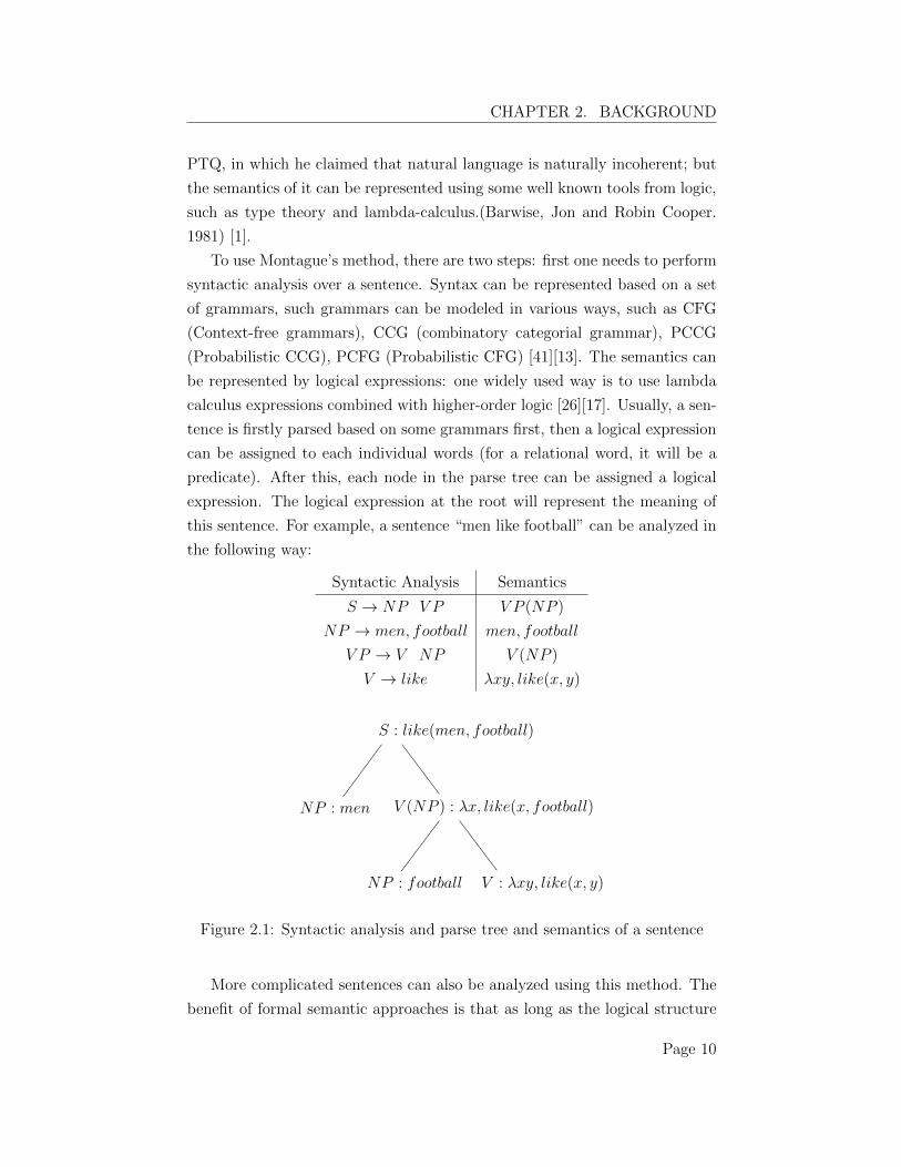
To use Montague’s method, there are two steps: first one needs to perform
syntactic analysis over a sentence. Syntax can be represented based on a set
of grammars, such grammars can be modeled in various ways, such as CFG
(Context-free grammars), CCG (combinatory categorial grammar), PCCG
(Probabilistic CCG), PCFG (Probabilistic CFG) [41][13]. The semantics can
be represented by logical expressions: one widely used way is to use lambda
calculus expressions combined with higher-order logic [26][17]. Usually, a sen-
tence is firstly parsed based on some grammars first, then a logical expression
can be assigned to each individual words (for a relational word, it will be a
predicate). After this, each node in the parse tree can be assigned a logical
expression. The logical expression at the root will represent the meaning of
this sentence. For example, a sentence “men like football” can be analyzed in
the following way:
Syntactic Analysis Semantics
S ! NP V P V P (NP )
NP ! men, football men, football
V P ! V NP V (NP )
V ! like �xy, like(x, y)
NP : football
V (NP ) : �x, like(x, football)
V : �xy, like(x, y)
S : like(men, football)
NP : men
Figure 2.1: Syntactic analysis and parse tree and semantics of a sentence
More complicated sentences can also be analyzed using this method. The
benefit of formal semantic approaches is that as long as the logical structure
Page 10
CHAPTER 2. BACKGROUND
of a sentence is obtained, the truth value of a sentence can be calculated. In
real world applications, this greatly helps analyze the inference of a sentence.
However, formal semantics is not really quantitative, and simply using
truth values cannot tell a lot of things, such as the similarity between words,
which can be calculated from distributional models described below. Formal
semantics also fails when a sentence is grammatically correct but has no sense
in term of semantics. For example, Chomsky’s example “colorless green ideas
sleep furiously” in his Syntactic Structures [2]. In other cases, such as id-
ioms and metaphors, where the semantic of a sentence is not exactly what it
suggests literally, formal semantics also will not work well. Moreover, formal
semantics approaches always su↵er from ambiguity of sentence, lack of context
data, and complexity issues in practice.
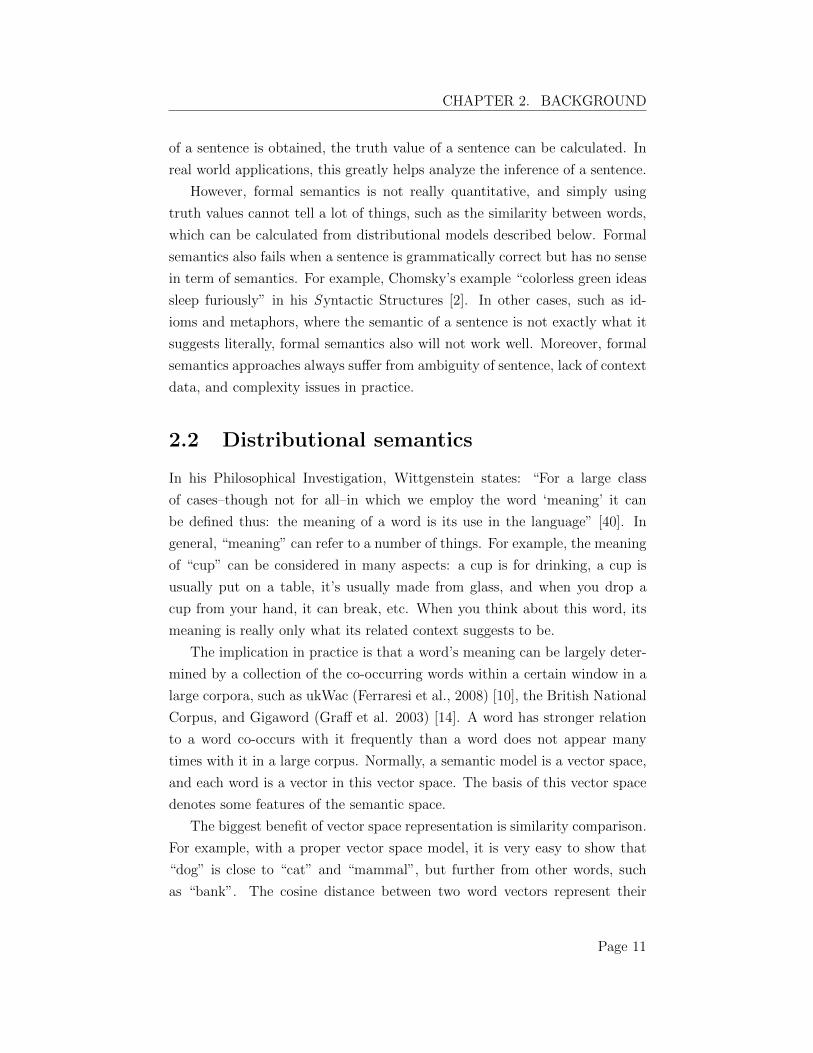
2.2 Distributional semantics
In his Philosophical Investigation, Wittgenstein states: “For a large class
of cases–though not for all–in which we employ the word ‘meaning’ it can
be defined thus: the meaning of a word is its use in the language” [40]. In
general, “meaning” can refer to a number of things. For example, the meaning
of “cup” can be considered in many aspects: a cup is for drinking, a cup is
usually put on a table, it’s usually made from glass, and when you drop a
cup from your hand, it can break, etc. When you think about this word, its
meaning is really only what its related context suggests to be.
The implication in practice is that a word’s meaning can be largely deter-
mined by a collection of the co-occurring words within a certain window in a
large corpora, such as ukWac (Ferraresi et al., 2008) [10], the British National
Corpus, and Gigaword (Gra↵ et al. 2003) [14]. A word has stronger relation
to a word co-occurs with it frequently than a word does not appear many
times with it in a large corpus. Normally, a semantic model is a vector space,
and each word is a vector in this vector space. The basis of this vector space
denotes some features of the semantic space.
The biggest benefit of vector space representation is similarity comparison.
For example, with a proper vector space model, it is very easy to show that
“dog” is close to “cat” and “mammal”, but further from other words, such
as “bank”. The cosine distance between two word vectors represent their
Page 11
CHAPTER 2. BACKGROUND
similarity. Given two words “cat” and “dog”, they can be expressed as�!cat and
�!dog in some semantic vector space, and their distance is
�!cat·
�!dog
k�!catkk�!dogk
. This model
has already been useful in many fields, such as word clustering, automatic
thesauri discovery, information retrieval and paraphrasing.
2.3 Compositionality in distributional models
of meaning
The two camps are thought to be orthogonal methods, and either of them has
pros and cons complementary to the other. In recent years, adding composi-
tional information to distributional models had been investigated.
The three basic models introduced below will be the baseline models in
the experiment later.
2.3.1 Additive models
The simplest idea is to add all word vectors in a sentence together, and produce
a new vector representing the sentence. The vector for a sentence containing
n words will be calculated as following:
���������!W1W2 . . .Wn
=nX
i=1
�!W
i
A simple example:
�������������������!Mike Studies Economies =
���!Mike+
�����!Studies+
�������!Economies
The additive model has been proved to be very e�cient in computing, and
has given good results in experiments [24]. The main problem of the additive
model is that the addition operation is commutative, therefore “cat catches
mouse” will be equal to “mouse catches cat”. However, this can be solved,
as stated in [24], by adding scalar factors to di↵erent words:���������!W1W2 . . .Wn
=P
n
i=1 ci�!W
i
, where {ci
}i
is a set of coe�cients. In this case, the result is never
Page 12
CHAPTER 2. BACKGROUND
commutative anymore, but how to determine the values of those scalar factors
is another problem.
2.3.2 Multiplicative models
The multiplicative model is also a so-called ”bag of words” model. Instead
of adding vectors, it point-wise multiplies all vectors in a sentence to produce
sentence vector.
���������!W1W2 . . .Wn
=nY
i=1
�!W
i
Again, a simple example can be:
�������������������!Mike Studies Economies =
���!Mike�
�����!Studies��������!
Economies
The multiplicative model still su↵ers from the commutative problem; and
by adding coe�cients to weight the individual words (as shown in the additive
model) will not solve this problem either. In addition, if the vectors are sparse,
the sentence vectors computed from point-wise multiplications will contain a
large number of zeros, which will make similarity comparison very imprecise.
In most cases this is not a desired property. The use of some smoothing tech-
niques can avoid too many zero entries in the resulted vectors [24]. Although
the multiplicative method is commutative, Edward Grefenstette [15] pointed
out that the multiplicative model evaluated in [24] shows better ability for
disambiguation on verbs. This is mainly because multiplication is an infor-
mation non-increasing process. As shown in the next chapter this property,
and the information non-decreasing property of the additive method can help
with modeling disjunctions and conjunctions.
2.3.3 Sentence living in tensor space
One elegant idea is to represent sentences as tensor products of words (Smolen-
sky, 1990, [24]). A sentence of n words can be represented by:
Page 13
CHAPTER 2. BACKGROUND
���������!W1W2 . . .Wn
=W1 ⌦W2 ⌦ · · ·⌦W
n
�������������������!Mike Studies Economies =
���!Mike⌦
�����!Studies⌦�������!
Economies
In this approach, sentence vectors live in higher dimensional spaces. Also
tensor product is non-commutative, so it does not have the bag-of-words mod-
els’ problem of commutative property.
In addition, Clark and Pulman further proposed the idea to embed word
types into the representation of vectors [3]. But long sentences produce higher
dimensional vectors, and sentences of di↵erent lengths will fall into vector
spaces of di↵erent orders. Therefore they will not be comparable to each
other. Both of these problems make this approach not feasible in practice.
2.3.4 Other models
Some research makes use of the topological structures of sentences, especially
in the applications where similarity comparison is important. In these meth-
ods, a sentence is firstly parsed by some dependency parser. The similarity of
two sentences depends on the common edges of the trees (word-overlap) [39].
Remarkably, Vasile Rus, et al. (2008) used a graph based model [29]. In their
paper, text is firstly converted into a graph according to some dependency-
graph formalism (text ! dependency graph). The graph is thus a represen-
tation of the sentence. After that, the sentence similarity problem is reduced
to a graph isomorphism search (graph subsumption or containment). Rus’
model obtained very positive results for paraphrasing.
Other feasible models have also been proposed. For example, many deep
learning based models have been developed recently. Socher et al. [34][35][36]
used recursive neural networks (RNN) that parse natural language sentences
and produce vectors for sentences based on compositionality. The model works
for sentences with variable sizes, and it works particularly well on identifying
negations. Their recursive auto-encoder model has been applied to paraphrase
detection and prediction of sentiment distribution, which also obtained very
Page 14

CHAPTER 2. BACKGROUND
good results [33][37].
Coecke et al. (2010) [6] proposed a categorical framework of meaning
which takes advantage of the fact that both a pregroup grammar and the
category of finite-dimensional vector spaces with linear maps share a compact
closed structure. The construction of a sentence vector from word vectors
is performed by tensor contraction. The framework preserves the order of
words, and more importantly, does not su↵er from the dimensionality expan-
sion problems of other tensor-product approaches, since the tensor contraction
process guarantees that every sentence vector will live in a basic vector space.
And the following section will introduce the categorical model in details.
2.4 A categorical framework of meaning
The categorical model provides a mathematical foundation of a compositional
distributional models of meaning. The essentiality of category theory here as
a passage is described in (Coecke et. al.) [6].
First I will start with the basic components will be used in this paper.
2.4.1 Category
A category C can be defined as following:
1. a collection of objects
2. a collection of morphisms (or arrows)
3. each morphism has domain (dom) A and codomain (cod) B, therefore a
morphism f can be written as f : A ! B
4. there is a composition operation � for each pair of arrows f, g, with
cod(f) = dom(g), g � f : dom(f) ! cod(g), composition operation satis-
fies the associative law.
5. for each object A, there is an identity morphism 1A
: A ! A. For any
morphism f : A ! B, there is f � 1A
= f , 1B
� f = f .
Based on this simple definition of category, many other categories can be
constructed with some additional structures. They have strong expressive
power to model many existing mathematical structures. For more details
about Category Theory itself, one can refer to Benjamin Pierece’s book [27].
Page 15
CHAPTER 2. BACKGROUND
2.4.2 Monoidal category
Another essential property we want to capture in natural language is the
“parallel composition”. A sentence “W1W2...Wm
” can be represented by ten-
sor W1 ⌦W2 ⌦ ...⌦W
m
. Each of these words can be a vector, or a tensor of
any order, and they are composed in parallel by monoidal tensor.
Here, each word can either live in a vector space of order 1, or live in a
higher-order vector space. The resulted sentence vector is the tensor prod-
uct of all words sequentially. To capture parallel composition, the feature of
monoidal category is useful.
A monoidal category is a category that admits monoidal tensor: For each
ordered pair of objects (A, B), there is a parallel composite object A ⌦ B,
where ⌦ is called the monoidal tensor. There is a unit object I in a monoidal
category, satisfying the following property:
A⌦ I = A = I ⌦ A
For each pair of morphisms (f : A ! B, g : C ! D), there is a parallel
composite morphism f ⌦ g : A⌦ C ! B ⌦D.
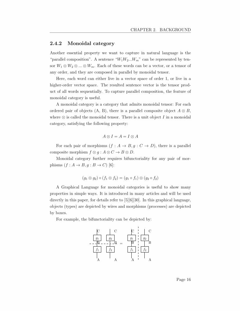
Monoidal category further requires bifunctoriality for any pair of mor-
phisms (f : A ! B, g : B ! C) [6]:
(g1 ⌦ g2) � (f1 ⌦ f2) = (g1 � f1)⌦ (g2 � f2)
A Graphical Language for monoidal categories is useful to show many
properties in simple ways. It is introduced in many articles and will be used
directly in this paper, for details refer to [5][6][30]. In this graphical language,
objects (types) are depicted by wires and morphisms (processes) are depicted
by boxes.
For example, the bifunctoriality can be depicted by:
g1
f1
g2
f2
g1
f1
g2
f2
=
A
B
C
A
B
C
A
B
C C
B
A
Page 16
CHAPTER 2. BACKGROUND
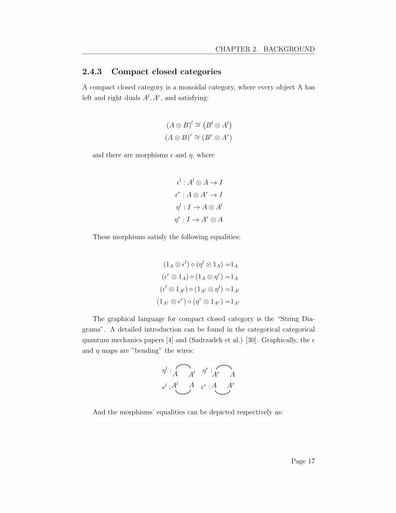
2.4.3 Compact closed categories
A compact closed category is a monoidal category, where every object A has
left and right duals Al
, A
r, and satisfying:
(A⌦ B)l ⇠=�B
l ⌦ A
l
�
(A⌦ B)r ⇠= (Br ⌦ A
r)
and there are morphisms ✏ and ⌘, where
✏
l : Al ⌦ A ! I
✏
r : A⌦ A
r ! I
⌘
l : I ! A⌦ A
l
⌘
r : I ! A
r ⌦ A
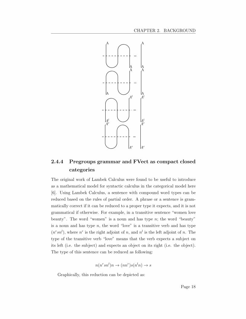
These morphisms satisfy the following equalities:
(1A
⌦ ✏
l) � (⌘l ⌦ 1A
) =1A
(✏r ⌦ 1A
) � (1A
⌦ ⌘
r) =1A
(✏l ⌦ 1A
l) � (1A
l ⌦ ⌘
l) =1A
l
(1A
r ⌦ ✏
r) � (⌘r ⌦ 1A
r) =1A
r
The graphical language for compact closed category is the “String Dia-
grams”. A detailed introduction can be found in the categorical categorical
quantum mechanics papers [4] and (Sadrzadeh et al.) [30]. Graphically, the ✏
and ⌘ maps are ”bending” the wires:
⌘
l :A
A
l
⌘
r :A
r
A
✏
l : A
A
l
✏
r : A
r
A
And the morphisms’ equalities can be depicted respectively as:
Page 17
CHAPTER 2. BACKGROUND
=
A
A A
A
=
A
A
A
A
=
Al
Al
Al
Al
=
Ar
Ar Ar
Ar
2.4.4 Pregroups grammar and FVect as compact closed
categories
The original work of Lambek Calculus were found to be useful to introduce
as a mathematical model for syntactic calculus in the categorical model here
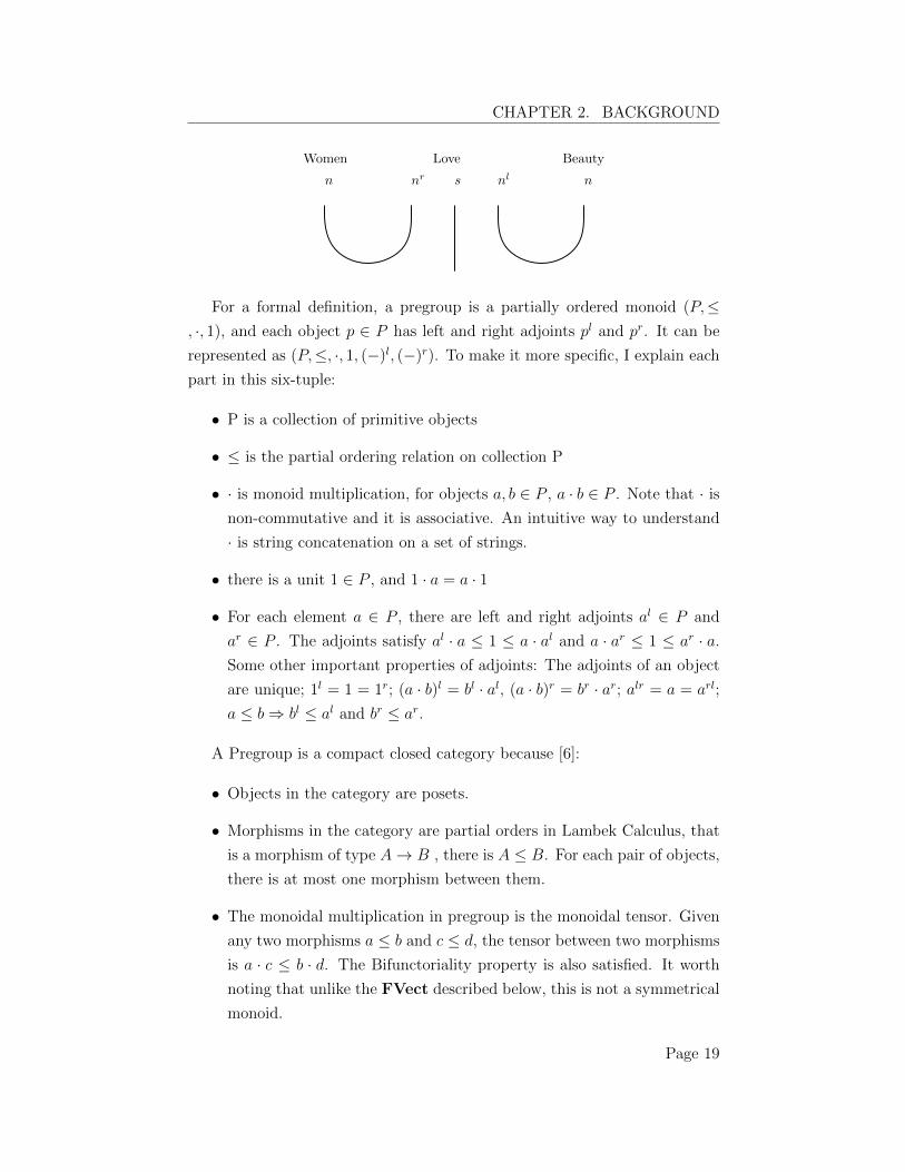
[6]. Using Lambek Calculus, a sentence with compound word types can be
reduced based on the rules of partial order. A phrase or a sentence is gram-
matically correct if it can be reduced to a proper type it expects, and it is not
grammatical if otherwise. For example, in a transitive sentence “women love
beauty”. The word “women” is a noun and has type n; the word “beauty”
is a noun and has type n, the word “love” is a transitive verb and has type
(nr
sn
l), where nr is the right adjoint of n, and n
l is the left adjoint of n. The
type of the transitive verb “love” means that the verb expects a subject on
its left (i.e. the subject) and expects an object on its right (i.e. the object).
The type of this sentence can be reduced as following:
n(nr
sn
l)n ! (nnr)s(nl
n) ! s
Graphically, this reduction can be depicted as:
Page 18
CHAPTER 2. BACKGROUND
s nlnr nn
Women Love Beauty
For a formal definition, a pregroup is a partially ordered monoid (P,, ·, 1), and each object p 2 P has left and right adjoints pl and p
r. It can be
represented as (P,, ·, 1, (�)l, (�)r). To make it more specific, I explain each
part in this six-tuple:
• P is a collection of primitive objects
• is the partial ordering relation on collection P
• · is monoid multiplication, for objects a, b 2 P , a · b 2 P . Note that · isnon-commutative and it is associative. An intuitive way to understand
· is string concatenation on a set of strings.
• there is a unit 1 2 P , and 1 · a = a · 1
• For each element a 2 P , there are left and right adjoints a
l 2 P and
a
r 2 P . The adjoints satisfy a
l · a 1 a · al and a · ar 1 a
r · a.Some other important properties of adjoints: The adjoints of an object
are unique; 1l = 1 = 1r; (a · b)l = b
l · al, (a · b)r = b
r · ar; alr = a = a
rl;
a b ) b
l a
l and b
r a
r.
A Pregroup is a compact closed category because [6]:
• Objects in the category are posets.
• Morphisms in the category are partial orders in Lambek Calculus, that
is a morphism of type A ! B , there is A B. For each pair of objects,
there is at most one morphism between them.
• The monoidal multiplication in pregroup is the monoidal tensor. Given
any two morphisms a b and c d, the tensor between two morphisms
is a · c b · d. The Bifunctoriality property is also satisfied. It worth
noting that unlike the FVect described below, this is not a symmetrical
monoid.
Page 19
CHAPTER 2. BACKGROUND
• Each object has left and right adjoints. The epsilon maps and eta maps
are: ✏
l : pl · p 1, ✏r : p · pr 1, ⌘l : 1 p · pl and ⌘
r : 1 p
r · p.They correspondes to the “cups” and “caps” in the graphically language
respectively.
FVect is the category where finite-dimensional vector spaces over R are
objects, linear maps are morphisms and vector space tensor is monoidal tensor
[6]. There is also inner product for the vector spaces. FVect is a compact
closed category when vector spaces on R are objects, linear maps between
vector spaces are morphisms, and vector space tensor product is monoidal
tensor, the unit is the scalars in R. There is also an isomorphism V1 ⌦ V2⇠=
V2 ⌦ V1 for any tensor objects V1 ⌦ V2 and V2 ⌦ V1. This makes FVect a
symmetrical monoidal category. Every vector space has a dual vector space
(conjugate transpose) V ⇤. Since the vector space is over R, the dual space is
its transpose, and V
⇠= V
⇤. Because of the symmetrical property of FVect,
the left adjoint and right adjoint of a vector space are the same, and they are
equal to its dual: V l = V
⇤ = V
r. We also assume that the vector spaces have
fixed basis {�!ni
}i
, and there is inner product over a vector space. The epsilon
and eta maps can be concretely defined as:
✏
l = ✏
r : V ⌦ V ! R ::X
ij
c
ij
�!n
i
⌦�!n
j
!X
ij
c
ij
h�!ni
|�!nj
i
⌘
l = ⌘
r : R ! V ⌦ V :: 1 !X
ij
c
ij
�!n
i
⌦�!n
j
The fact that FVect is a compact closed category can then be verified
[6][15].
2.4.5 A passage from syntax to semantics
The previous subsection has shown that the Pregroups Grammars and Vector
spaces with linear maps share the same compact closed structure. The cat-
egorical framework unites these two important aspects of natural language:
compositional information represented by grammar and meaning represented
by vector space. In practice, this means that a sentence’s grammatical struc-
ture can be reduced based on the word types and rules in the grammar, and
this can be a guidance of how the tensor of a sentence can be reduced to a
Page 20
CHAPTER 2. BACKGROUND
basic order-1 vector. This takes into account the composition information of
a sentence, in the same time it reduces sentence vector into a basic vector
(order 1), solved the dimensionality problem.
In the original work of (Coecke et al.) [6], the “meaning” of language is
considered to be the product category FVect ⇥ P , in which a pair of vector
space and grammar type (V, a) is an object and a pair of linear map and
pregroup order relation (f,) is a morphism. This product category is also
a compact closed category. In particular, there are four morphisms: (✏l,),
(✏r,), (⌘l,) and (⌘r,). The sentence’s type can be reduced based on the
grammar, and the corresponding vector space linear maps are applied to the
words’ vectors. Concrete examples of di↵erent types of phrases and sentences
will be given in the Methodology Chapter.
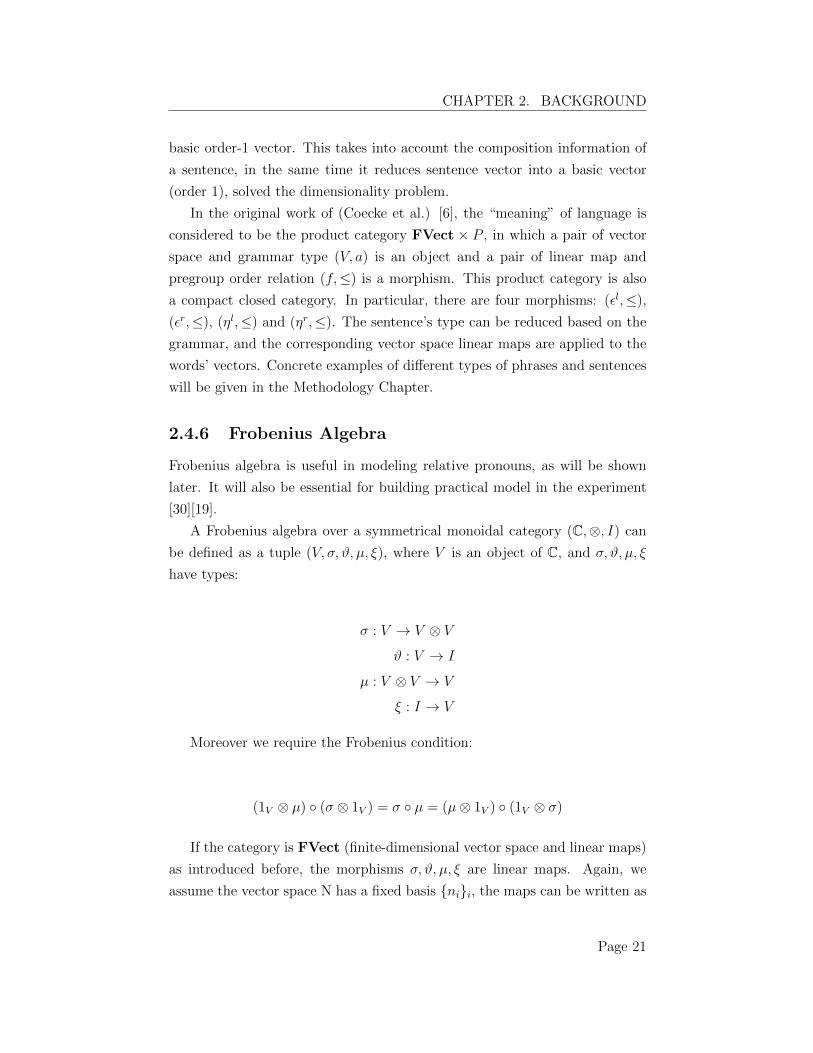
2.4.6 Frobenius Algebra
Frobenius algebra is useful in modeling relative pronouns, as will be shown
later. It will also be essential for building practical model in the experiment
[30][19].
A Frobenius algebra over a symmetrical monoidal category (C,⌦, I) can
be defined as a tuple (V, �,#, µ, ⇠), where V is an object of C, and �,#, µ, ⇠
have types:
� : V ! V ⌦ V
# : V ! I
µ : V ⌦ V ! V
⇠ : I ! V
Moreover we require the Frobenius condition:
(1V
⌦ µ) � (� ⌦ 1V
) = � � µ = (µ⌦ 1V
) � (1V
⌦ �)
If the category is FVect (finite-dimensional vector space and linear maps)
as introduced before, the morphisms �,#, µ, ⇠ are linear maps. Again, we
assume the vector space N has a fixed basis {ni
}i
, the maps can be written as
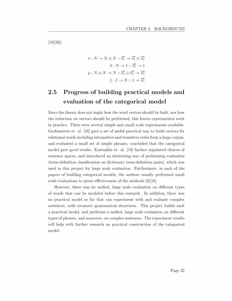
Page 21
CHAPTER 2. BACKGROUND
[19][30]:
� : N ! N ⌦N :: �!ni
! �!n
i
⌦�!n
i
# : N ! I :: �!ni
! 1
µ : N ⌦N ! N :: �!ni
⌦�!n
i
! �!n
i
⇠ : I ! N :: 1 ! �!n
i
2.5 Progress of building practical models and
evaluation of the categorical model
Since the theory does not imply how the word vectors should be built, nor how
the reduction on vectors should be performed, this leaves experimental work
in practice. There were several simple and small scale experiments available.
Grefenstette et. al. [16] gave a set of useful practical way to build vectors for
relational words including intransitive and transitive verbs from a large corpus,
and evaluated a small set of simple phrases, concluded that the categorical
model gave good results. Kartsaklis et. al. [19] further stipulated choices of
sentence spaces, and introduced an interesting way of performing evaluation
(term-definition classification on dictionary term-definition pairs), which was
used in this project for large scale evaluation. Furthermore, in each of the
papers of building categorical models, the authors usually performed small
scale evaluations to prove e↵ectiveness of the methods [6][16].
However, there was no unified, large scale evaluation on di↵erent types
of words that can be modeled before this research. In addition, there was
no practical model so far that can experiment with and evaluate complex
sentences, with recursive grammatical structures. This project builds such
a practical model, and performs a unified, large scale evaluation on di↵erent
types of phrases, and moreover, on complex sentences. The experiment results
will help with further research on practical construction of the categorical
model.
Page 22
Chapter 3
Methodology
In this section, a set of practical solutions of building the categorical model
are provided. First di↵erent semantic word spaces are introduced, then the
particular ways of creating vectors for di↵erent types of relational words in
this paper. Lastly, I introduce the details of implementing the model, which
will be used in the experimental work in the next chapter.
3.1 Semantic word spaces for the categorical
model
Semantic word space is the basic building block of distributional semantic
models, and the tensor spaces for relational words are built upon the basic
semantic word spaces.
A semantic word space is a vector space of words’ semantics, in which each
word is represented by a vector. Each dimension of the vector space represents
one certain feature. In a conventional vector space, each dimension of a word
vector is the co-occurrence count of another word within a window over a
large corpora. The vector space used in this project is from an experiment
conducted by Kartsaklis et al. [18]. The vectors were trained from the ukWaC
corpus (Ferraresi et al. 2008) [10], and used 2000 content words (excluding
the 50 most frequent “stop” words) as the basis. The context is set up to be
a 5-word window from each side of the target word. A vector is created for
every content word that has at least 100 occurrences in the ukWaC corpus.
The semantic space is scored 0.77 Spearman’s rank correlation coe�cient (i.e.
Spearman’s ⇢) on a benchmark dataset of Rubenstein and Goodenough (1965)
23
CHAPTER 3. METHODOLOGY
[18][28]. In the vector space, each word has a tag to denote its type. There are
four types of words: noun, verb, adjective, and adverb. All vectors contain
only positive numbers.
There are also other types of semantic word spaces being built so far.
One popular type of semantic vectors is the so called neural vectors using
machine learning techniques, such as neural networks. These models usually
produce decent word vector spaces of relatively low dimensions ( 300). I
experimented two neural vector spaces during a very early stage of this project:
The vector space trained by Turian et al. [38], which implemented the model
introduced by Collobert and Weston (2008) [7], as well as the Word2Vec tool
developed by Mikolov et al. [23]. However, having negative values is not a
desired property in the multiplicative model, and hence the categorical model.
This result will be shown in the experiment chapter.
It was also experimented by Kartsaklis et al. [18] to reduce the original
vector space to a 300 dimensional vector space using Singular Vector Decom-
position (SVD). After the SVD process, the vector space has a much lower
dimension (300), but introduces negative numbers as well. Thus in the exper-
iment, I used the vector space before SVD, which is 2000-dimensional.
3.2 Sentence space
As the categorical framework actually does not imply a particular sentence
space, Kartsaklis et. al. [19] gave a clear comparison of two feasible sentence
spaces in practice: S = N ⌦N and S = N [19]. When sentences are instan-
tiated on S = N ⌦ N , it comes with the problem that sentences of di↵erent
grammatical structure and di↵erent lengths will have vectors of di↵erent or-
ders. This will cause troubles when comparing arbitrary sentences. In this
project, sentence vectors of order 1 (S = N) will be preferred because of its
ability to compare sentences of any grammatical structures in the basic vector
space, by calculating the cosine distance between these vectors. In the later
session “Implementation Details”, I will explain how a an arbitrary sentence
can be reduced to a basic vector based on the categorical framework with
some simplification described below.
Page 24
CHAPTER 3. METHODOLOGY
3.3 Create tensors for relational words
Another practical issue that the categorical framework does not specify is
how the tensors for relational words are created. For example, the matrix for
adjectives and the order-3 tensors (“cubes”) for transitive verbs, etc. As the
pregroup types of words show in the background chapter, there are basic order-
1 vectors (usually the nouns), and there are multi-linear maps (the relational
words, usually functional words such as verbs, adjectives, etc.). The relational
words should be “applied” to other words, and they are tensors of higher
orders.
This research focuses on creating tensor spaces directly from corpus. Grefen-
stette et. al. introduced a general way to create vectors for relational words
in [16]. It specifically discussed how the tensors for intransitive words and
transitive words can be trained from a corpus: in the intransitive case, the
subjects of the intransitive words were added together in the corpus, in the
transitive case, tensor of each subject-object pair of the transitive verb in a
corpus is added.
It is worth noting that in the original theory, an intransitive verb is a
matrix and a transitive verb is a tensor of order 3 (“a cube”). The method
mentioned above creates tensors that are one-order less than it supposes to be.
To solve this problem, one way is to directly construct higher-order vectors
is to add the verb itself in the tensor product, another way is to use machine
learning techniques to help construct the tensors. Considering the time and
space required for the first approach, these two methods are not included in
the scope of this experiment.
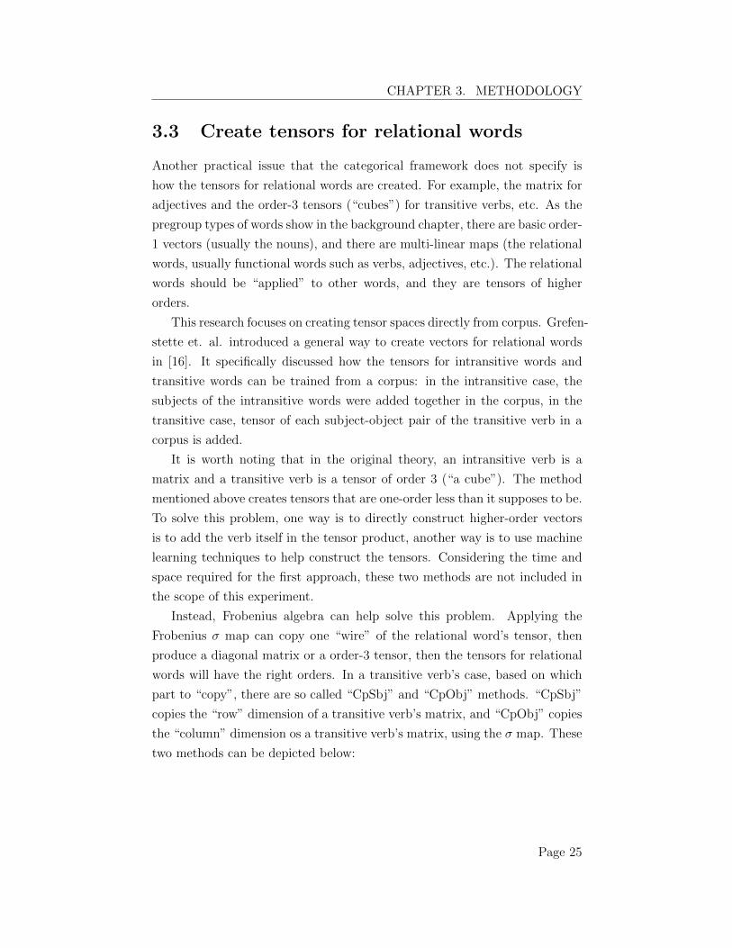
Instead, Frobenius algebra can help solve this problem. Applying the
Frobenius � map can copy one “wire” of the relational word’s tensor, then
produce a diagonal matrix or a order-3 tensor, then the tensors for relational
words will have the right orders. In a transitive verb’s case, based on which
part to “copy”, there are so called “CpSbj” and “CpObj” methods. “CpSbj”
copies the “row” dimension of a transitive verb’s matrix, and “CpObj” copies
the “column” dimension os a transitive verb’s matrix, using the � map. These
two methods can be depicted below:
Page 25
CHAPTER 3. METHODOLOGY
CpSbj CpObj
However, we suspect later this simplification will a↵ect the performance
in practice.
Based on the models and techniques introduced so far, we can now extend
the model to many other concrete types of words.
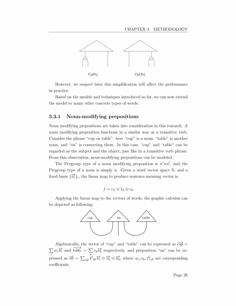
3.3.1 Noun-modifying prepositions
Noun modifying prepositions are taken into consideration in this research. A
noun modifying preposition functions in a similar way as a transitive verb.
Consider the phrase “cup on table”: here “cup” is a noun, “table” is another
noun, and “on” is connecting them. In this case, “cup” and “table” can be
regarded as the subject and the object, just like in a transitive verb phrase.
From this observation, noun-modifying prepositions can be modeled.
The Pregroup type of a noun modifying preposition is n
r
nn
l, and the
Pregroup type of a noun is simply n. Given a word vector space N, and a
fixed basis {�!ni
}i
, the linear map to produce sentence meaning vector is:
f = ✏N ⌦ 1S ⌦ ✏N
Applying the linear map to the vectors of words, the graphic calculus can
be depicted as following:
cup on table
Algebraically, the vector of “cup” and “table” can be expressed as �!cup =Pi
wi�!ni and
��!table =
Pk
vk�!nk respectively, and preposition “on” can be ex-
pressed as �!on =
Pijk
P ijk�!ni ⌦ �!
nj ⌦ �!nk, where w
i
, v
k
, P
ijk
are corresponding
coe�cients.
Page 26
CHAPTER 3. METHODOLOGY
Applying the linear map f to the tensor of word vectors:
f
⇣�!cup⌦�!
on⌦��!table
⌘
=✏
r
N
⌦ 1N
⌦ ✏
l
N
h�!cup⌦�!
on⌦��!table
i
=✏
r
N
⌦ 1N
⌦ ✏
l
N
" X
i
m
i
�!n
i
!⌦ X
ijk
P
ijk
�!n
i
⌦�!n
j
⌦�!n
k
!⌦ X
k
v
k
�!n
k
!#
=✏
r
N
⌦ 1N
⌦ ✏
l
N
"X
ijk
P
ijk
m
i
v
k
�!n
i
⌦�!n
i
⌦�!n
j
⌦�!n
k
⌦�!n
k
#
=X
ijk
P
ijk
✏
r
N
(�!ni
⌦�!n
i
)⌦ 1N
(�!nj
)⌦ ✏
l
N
(�!nk
⌦�!n
k
)
=X
ijk
P
ijk
m
i
v
k
h�!ni
|�!ni
i ⌦ �!n
j
⌦ h�!nk
|�!nk
i
=X
ijk
P
ijk
m
i
v
k
1⌦�!n
j
⌦ 1
⇠=X
ijk
P
ijk
m
i
v
k
�!n
j
The above equation is exactly �!cup ⇥
⇣�!on⇥
��!table
⌘T
. However, due to the
di�culty of creating order-3 tensors for relational words, in practical, Frobe-
nius models are used in this experiment. Since there is no particular emphasis
on either using CpSbj or using CpObj, the final vector is the addition (hence
average in cosine distance sense) of two vectors from CpSubj and CpObj. In
the CpSubj case, the derivation of “cup on table” is:
Page 27
CHAPTER 3. METHODOLOGY
µ
N
⌦ ✏
l
⇥�!cup⌦�!
on⌦��!table
⇤
=µ
N
⌦ ✏
l
⇥ X
i
mi�!n
i
!⌦ X
ijk
P
ik
�!n
i
⌦�!n
k
!⌦X
k
v
k
�!n
k
⇤
= µ
N
⌦ ✏
l
⇥X
ijk
P
ik
m
i
vk�!ni ⌦�!
ni ⌦�!nk ⌦�!
nk
⇤
=X
ik
P
ik
m
i
v
k
µ
N
(�!ni ⌦�!ni )⌦ ✏
l
N
(�!nk
⌦�!n
k
)
=X
ik
P
ik
m
k
v
k
�!n
i
⌦ 1
⇠=X
ik
P
ik
m
i
v
k
�!n
i
= �!cup�
⇣�!on⇥
��!table
⌘T
The commutative diagram is:
N ⌦N
r ⌦N
l ⌦N
1N
⌦ �
r
N
⌦ 1N
⌦ 1N
N ⌦N
r ⌦N
r ⌦N
l ⌦N
✏
r
N
⌦ 1rN
⌦ ✏
l
N
N
r ⇠= N
�µ
N
⌦ ✏
l
N
�
�✏
r
N
⌦ 1N
⌦ ✏
l
N
�� (1
N
⌦ �
N
⌦ 1⌦ 1)
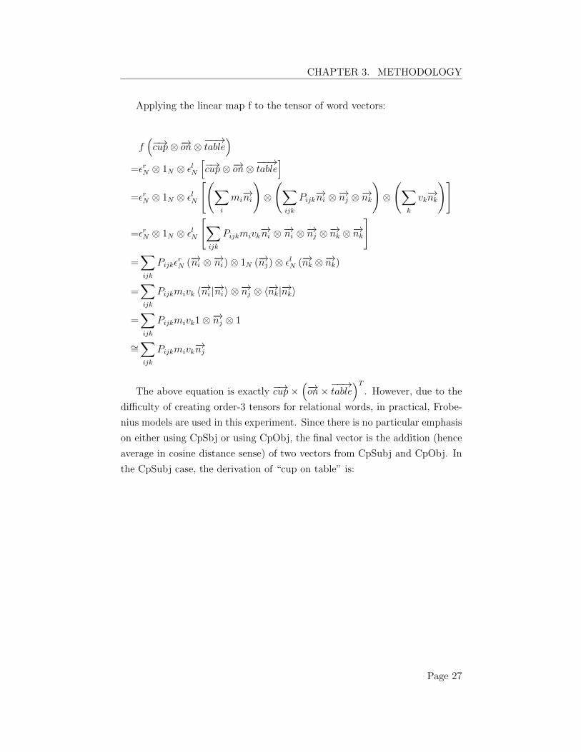
Graphically, CpSubj is depicted as below:
R OS
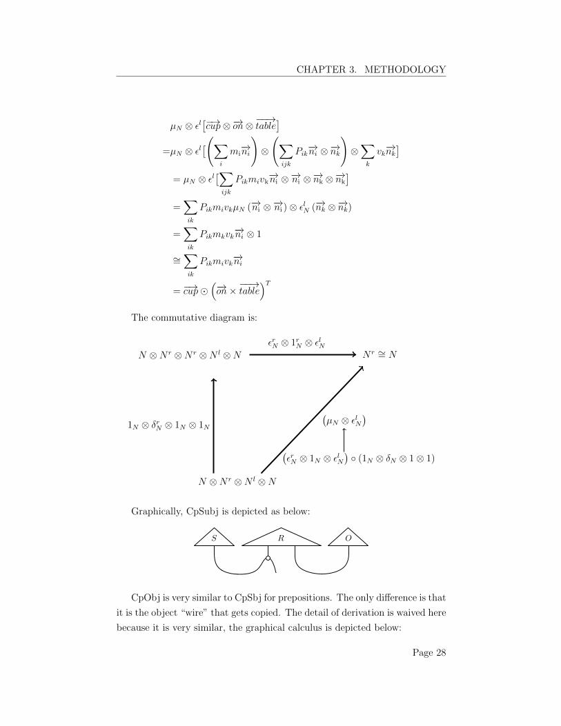
CpObj is very similar to CpSbj for prepositions. The only di↵erence is that
it is the object “wire” that gets copied. The detail of derivation is waived here
because it is very similar, the graphical calculus is depicted below:
Page 28
CHAPTER 3. METHODOLOGY
R OS
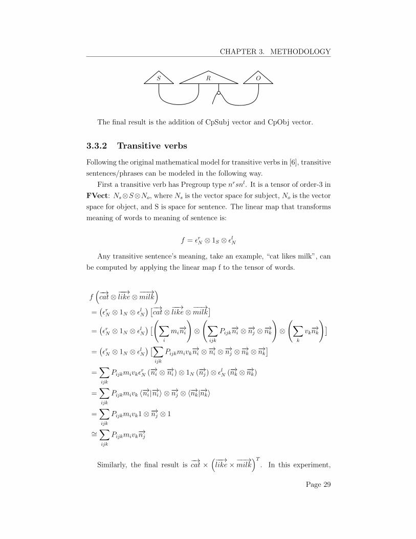
The final result is the addition of CpSubj vector and CpObj vector.
3.3.2 Transitive verbs
Following the original mathematical model for transitive verbs in [6], transitive
sentences/phrases can be modeled in the following way.
First a transitive verb has Pregroup type nr
sn
l. It is a tensor of order-3 in
FVect: Ns
⌦S⌦N
o
, where Ns
is the vector space for subject, No
is the vector
space for object, and S is space for sentence. The linear map that transforms
meaning of words to meaning of sentence is:
f = ✏
r
N
⌦ 1S
⌦ ✏
l
N
Any transitive sentence’s meaning, take an example, “cat likes milk”, can
be computed by applying the linear map f to the tensor of words.
f
⇣�!cat⌦
��!like⌦
��!milk
⌘
=�✏
r
N
⌦ 1N
⌦ ✏
l
N
� ⇥�!cat⌦
��!like⌦
��!milk
⇤
=�✏
r
N
⌦ 1N
⌦ ✏
l
N
� ⇥ X
i
m
i
�!n
i
!⌦ X
ijk
P
ijk
�!n
i
⌦�!n
j
⌦�!n
k
!⌦ X
k
v
k
�!n
k
!⇤
=�✏
r
N
⌦ 1N
⌦ ✏
l
N
� ⇥X
ijk
P
ijk
m
i
v
k
�!n
i
⌦�!n
i
⌦�!n
j
⌦�!n
k
⌦�!n
k
⇤
=X
ijk
P
ijk
m
i
v
k
✏
r
N
(�!ni
⌦�!n
i
)⌦ 1N
(�!nj
)⌦ ✏
l
N
(�!nk
⌦�!n
k
)
=X
ijk
P
ijk
m
i
v
k
h�!ni
|�!ni
i ⌦ �!n
j
⌦ h�!nk
|�!nk
i
=X
ijk
P
ijk
m
i
v
k
1⌦�!n
j
⌦ 1
⇠=X
ijk
P
ijk
m
i
v
k
�!n
j
Similarly, the final result is�!cat ⇥
⇣��!like⇥
��!milk
⌘T
. In this experiment,
Page 29
CHAPTER 3. METHODOLOGY
again, the Frobenius model are more suitable in practice. The final vector is
the addition of two vectors from CpSubj and CpObj. In the CpSubj case, the
derivation of ”cat likes milk” is:
�µ
N
⌦ ✏
l
� ⇥�!cat⌦
��!like⌦
��!milk
⇤
= (µN
⌦ ✏
l
)⇥ X
i
mi�!n
i
!⌦ X
ik
P
ik
�!n
i
⌦�!n
k
!⌦ X
k
v
k
�!n
k
!⇤
=�µ
N
⌦ ✏
l
� ⇥X
ijk
P
i
km
i
vk�!ni ⌦�!
ni ⌦�!nk ⌦�!
nk
⇤
=X
ik
P
ik
m
i
v
k
µ
N
(�!ni ⌦�!ni )⌦ ✏
l
N
(�!nk
⌦�!n
k
)
=X
ik
P
ik
m
k
v
k
�!n
i
⌦ 1
⇠=X
ik
P
ik
m
i
v
k
�!n
i
=�!cat�
⇣��!like⇥
��!milk
⌘T
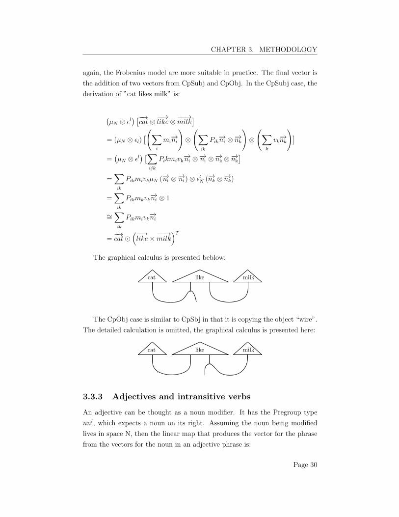
The graphical calculus is presented beblow:
cat like milk
The CpObj case is similar to CpSbj in that it is copying the object “wire”.
The detailed calculation is omitted, the graphical calculus is presented here:
cat like milk
3.3.3 Adjectives and intransitive verbs
An adjective can be thought as a noun modifier. It has the Pregroup type
nn
l, which expects a noun on its right. Assuming the noun being modified
lives in space N, then the linear map that produces the vector for the phrase
from the vectors for the noun in an adjective phrase is:
Page 30
CHAPTER 3. METHODOLOGY
f = 1N ⌦ ✏
l
N
Take a very simple example phrase “red goat”, given a fixed basis {�!ni
}i
,
the two words can be represented by:
�!red =
X
ij
A
ij
�!n
i
⌦�!n
j
��!goat =
X
j
m
j
�!n
j
By applying the linear map f to the meaning space of the adjective phrase,
the result can be derived in the following way:
�I
N
⌦ ✏
l
N
� h�!red⌦��!
goat
i
=�I
N
⌦ ✏
l
N
�" X
ij
A
ij
�!n
i
⌦�!n
j
!⌦ X
j
m
j
�!n
j
!#
=�I
N
⌦ ✏
l
N
�"X
ij
A
ij
m
j
�!n
i
⌦�!n
j
⌦�!n
j
#
=X
ij
A
ij
m
j
I
N
⇣�!n
i
⌘⌦ ✏
l
N
⇣�!n
j
⌦�!n
j
⌘
=X
ij
A
ij
m
j
�!n
i
⌦ h�!nj
|�!nj
i
=X
ij
A
ij
m
j
�!n
i
⌦ 1
=�!red⇥��!
goat
T
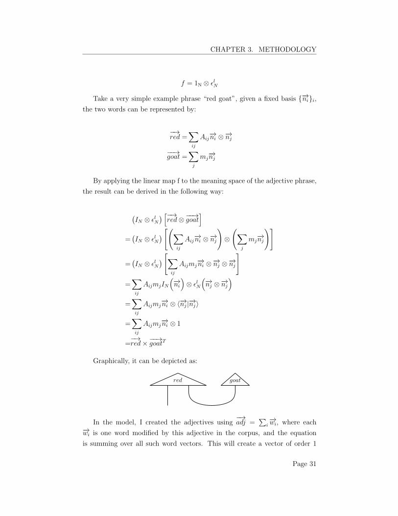
Graphically, it can be depicted as:
red goat
In the model, I created the adjectives using�!adj =
Pi
�!w
i
, where each�!w
i
is one word modified by this adjective in the corpus, and the equation
is summing over all such word vectors. This will create a vector of order 1
Page 31
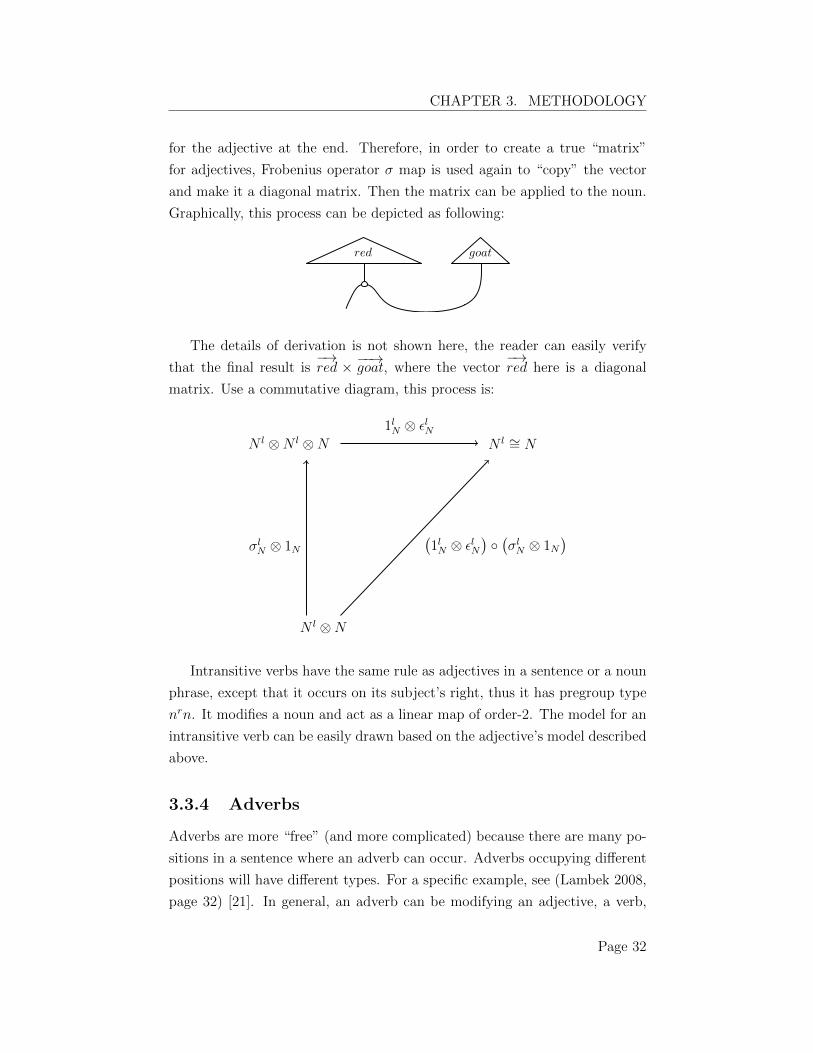
CHAPTER 3. METHODOLOGY
for the adjective at the end. Therefore, in order to create a true “matrix”
for adjectives, Frobenius operator � map is used again to “copy” the vector
and make it a diagonal matrix. Then the matrix can be applied to the noun.
Graphically, this process can be depicted as following:
red goat
The details of derivation is not shown here, the reader can easily verify
that the final result is�!red ⇥ ��!
goat, where the vector�!red here is a diagonal
matrix. Use a commutative diagram, this process is:
N
l ⌦N
�
l
N
⌦ 1N
N
l ⌦N
l ⌦N
1lN
⌦ ✏
l
N
N
l ⇠= N
�1lN
⌦ ✏
l
N
����
l
N
⌦ 1N
�
Intransitive verbs have the same rule as adjectives in a sentence or a noun
phrase, except that it occurs on its subject’s right, thus it has pregroup type
n
r
n. It modifies a noun and act as a linear map of order-2. The model for an
intransitive verb can be easily drawn based on the adjective’s model described
above.
3.3.4 Adverbs
Adverbs are more “free” (and more complicated) because there are many po-
sitions in a sentence where an adverb can occur. Adverbs occupying di↵erent
positions will have di↵erent types. For a specific example, see (Lambek 2008,
page 32) [21]. In general, an adverb can be modifying an adjective, a verb,
Page 32
CHAPTER 3. METHODOLOGY
a preposition or a sentence, depending on where the adverb occurs in that
sentence.
Take an intransitive verb-modifying adverb for an example: the adverb
has type (nr
s)r(nr
s) ! s
r
n
rr
n
r
s if it is on the right side of the verb; it has
type (nr
s)(nr
s)l ! n
r
ss
l
n. Adjective-modifying adverbs have similar types.
Here an adverb is a order-4 tensor in FVect. When an adverb is modifying a
transitive verb, it is a order-6 tenor.
An adverb can also be a sentence modifier. In this case, an adverb can
have type s
r
s or ss
l, depending on which side of the sentence this adverb
appears. Since a sentence is instantiated on a basic vector, an adverb is a
matrix in this case.
One interesting simplification that is worth noticing is from Lambek [20][22].
It assigns an adverb a basic type ↵. Any other word modified by an adverb is
thus reduced to its own type: give a word of any type t, t↵ t and ↵t t [20].
However, this does not give us freedom in terms of vector spaces, since the
type ↵ can represent tensors of di↵erent orders in a real sentence depending
on what it modifies.
A order-4 or a order-6 tensor is not feasible to build in practice because
of the training time and space requirements. We need some simplification
on adverbs. First of all, verb-modifying adverbs are not considered in this
project. From the dataset, there are a few adjective-modifying adverbs and
sentence-modifying adverbs. We will only consider these two here.
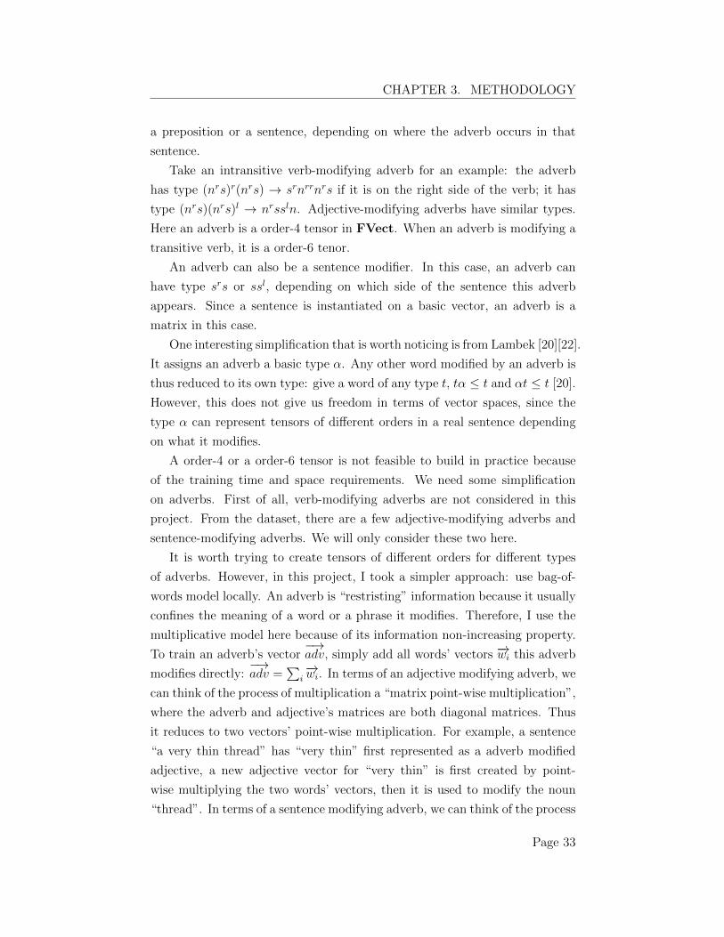
It is worth trying to create tensors of di↵erent orders for di↵erent types
of adverbs. However, in this project, I took a simpler approach: use bag-of-
words model locally. An adverb is “restristing” information because it usually
confines the meaning of a word or a phrase it modifies. Therefore, I use the
multiplicative model here because of its information non-increasing property.
To train an adverb’s vector�!adv, simply add all words’ vectors �!w
i
this adverb
modifies directly:�!adv =
Pi
�!w
i
. In terms of an adjective modifying adverb, we
can think of the process of multiplication a “matrix point-wise multiplication”,
where the adverb and adjective’s matrices are both diagonal matrices. Thus
it reduces to two vectors’ point-wise multiplication. For example, a sentence
“a very thin thread” has “very thin” first represented as a adverb modified
adjective, a new adjective vector for “very thin” is first created by point-
wise multiplying the two words’ vectors, then it is used to modify the noun
“thread”. In terms of a sentence modifying adverb, we can think of the process
Page 33
CHAPTER 3. METHODOLOGY
of multiplication a vector point-wise multiplication. For example, a sentence
“Quickly, we believed him”. In this case, the final sentence vector created
can be point-wise multiplication of the adverb “quickly” and the vector of the
sentence “we believed him”.
3.3.5 Compound verb
In real sentences, compound verbs are often used. There are di↵erent types
of compound verbs. Here I give a few examples:
• Prepositional verbs: “rely on”, “climb over”. Here the prepositions are
acting as normal prepositions and they are used together with verbs to
apply on particular objects.
• Phrasal verbs: “break down”, “work out”. Here the prepositions are
acting like adverbs.
• A compound single word as a verb: “water-proof”
• Verbs with Auxiliaries: Examples are “am thinking”, “have been doing”.
In the first two cases, a transitive verb-modifying preposition has type
(nr
sn
l)r(nr
sn
l). It is a order-6 tensor in FVect. Again I did a simplification
by using the additive model on such cases locally. Both a transitive verb and
a preposition live in the same order-3 tensor space as linear maps. Therefore,
I treat a prepositional verb as a new verb that is close to both to the verb and
the preposition. Similar to the adverbs, for simplification, vector addition is
used here. For example, the vector for the prepositional verb “rely on” will
be (��!rely + �!
on). There are a few prepositional verbs and phrasal verbs in the
experimental dataset.
A compound single word is treated as a single verb in this project. If such
a verb occurs in the BNC corpus, it will be considered as one word, therefore
it makes no di↵erence from a normal verb.
Verbs with auxiliaries are not considered in this research.
3.3.6 Relative pronouns
The work of (Sadrzadeh et. al) [30][31] gave a very detailed explanation in
their two papers to model relative pronouns. In the first paper, subject and
Page 34
CHAPTER 3. METHODOLOGY
object relative pronouns were modeled [30], in the second paper, possessive
relative pronouns were modeled [31]. In this research, I followed the models
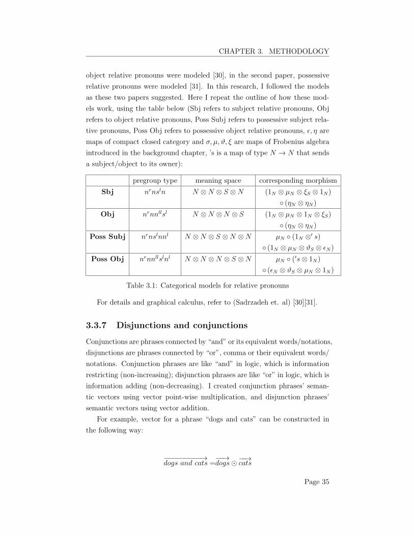
as these two papers suggested. Here I repeat the outline of how these mod-
els work, using the table below (Sbj refers to subject relative pronouns, Obj
refers to object relative pronouns, Poss Subj refers to possessive subject rela-
tive pronouns, Poss Obj refers to possessive object relative pronouns, ✏, ⌘ are
maps of compact closed category and �, µ,#, ⇠ are maps of Frobenius algebra
introduced in the background chapter, ’s is a map of type N ! N that sends
a subject/object to its owner):
pregroup type meaning space corresponding morphism
Sbj n
r
ns
l
n N ⌦N ⌦ S ⌦N (1N
⌦ µ
N
⌦ ⇠
S
⌦ 1N
)
� (⌘N
⌦ ⌘
N
)
Obj n
r
nn
ll
s
l
N ⌦N ⌦N ⌦ S (1N
⌦ µ
N
⌦ 1N
⌦ ⇠
S
)
� (⌘N
⌦ ⌘
N
)
Poss Subj n
r
ns
l
nn
l
N ⌦N ⌦ S ⌦N ⌦N µ
N
� (1N
⌦0s)
� (1N
⌦ µ
N
⌦ #
S
⌦ ✏
N
)
Poss Obj n
r
nn
ll
s
l
n
l
N ⌦N ⌦N ⌦ S ⌦N µ
N
� (0s⌦ 1N
)
� (✏N
⌦ #
S
⌦ µ
N
⌦ 1N
)
Table 3.1: Categorical models for relative pronouns
For details and graphical calculus, refer to (Sadrzadeh et. al) [30][31].
3.3.7 Disjunctions and conjunctions
Conjunctions are phrases connected by “and” or its equivalent words/notations,
disjunctions are phrases connected by “or”, comma or their equivalent words/
notations. Conjunction phrases are like “and” in logic, which is information
restricting (non-increasing); disjunction phrases are like “or” in logic, which is
information adding (non-decreasing). I created conjunction phrases’ seman-
tic vectors using vector point-wise multiplication, and disjunction phrases’
semantic vectors using vector addition.
For example, vector for a phrase “dogs and cats” can be constructed in
the following way:
���������!dogs and cats =
��!dogs���!
cats
Page 35
CHAPTER 3. METHODOLOGY
A disjunction phrase “year, month, hour” can be constructed in the fol-
lowing way:
������������!year month hour =��!
year +����!month+
��!hour
I consider a conjunction/disjunction phrase as a “compound” word/phrase
that is an average of all the individual components in it. Therefore, vector
point-wise multiplication and addition for such phrases inside a categorical
framework is reasonable in practice.
3.3.8 Sentence vs. phrase
In all the above discussions, we assumed that we were mostly working on
sentences: the types finally reduce to sentence type s. In the experiment,
all definitions from the dictionary are essentially noun phrases since they are
defining nouns. The only di↵erence we are going to make, is to replace s type
with n type when it is necessary.
3.4 Implementation of a practical categorical
model
This section will introduce how the relational word vectors were trained from
the British National Corpus (BNC), then outline the specific way in this
project to parse sentences/phrases so that the evaluation can be performed
accurately. Lastly, I will introduce the algorithm that takes the parse infor-
mation for a sentence, and computes the sentence vector.
3.4.1 Corpus for training
There are multiple large English corpus available for facilitating Computa-
tional Linguistics/NLP tasks. I adopted the British National Corpus (BNC),
with CCG (combinatory categorial grammar) parsing information 1. The BNC
has about 100 million words, selected from a wide range of written and spoken
1This corpus data was given by Dimitri Kartsaklis and Edward Grefenstette from theComputational Linguistics Group of Oxford University Computer Science Department.
Page 36
CHAPTER 3. METHODOLOGY
sources. The version I obtained is a CCG parsed BNC corpus available at the
Computational Linguistics Group of Oxford Computer Science Department.
CCG is very similar to pregoup grammars in structure, and additional infor-
mation is given in the corpus to help identify the words’ types and relations.
3.4.2 Train transitive verb matrices
A matrix for a transitive verb was trained by summing all subject/object ten-
sors with which the transitive verb appeared in the corpus:P
i
subject
i
⌦object
i
. This can be achieved by a simple algorithm. However scanning
through the BNC and constructing the matrices is time consuming. When
the 2000-dimensional word vectors are used, the space for each verb’s matrix
is huge. Because the nature of this project is an evaluation of the categorical
model, I only need to create matrices for less than 200 verbs. The strategy
used in the training process was to store every verb’s matrix in a separate file
to avoid a single, oversized file (shelve file) for all verb matrices. However,
this will not be practical in any real-world applications, thus reducing the
dimensionality of the word vector space is a necessary task (e.g. performing
non-negative matrix factorization). If the dimension of the word vectors is
300, then the size of a matrix is reduced from 20002 to 3002 in terms of the
number of entries.
3.4.3 “Direct tensor”: another way to create transitive
verb’s tensor
Instead creating a transitive verb’s tensor using the method introduced in
previous subsection, there is a simple way. For each transitive verb v in
the semantic word vector space, its matrix can be directly created by v ⌦v. This approach gave di↵erent but consistent results. As shown in the
experimental work chapter, I will denote this method as “VT-Direct” and
denote the method introduced in the previous section as “VT-BNC”.
3.4.4 Train preposition matrices
Training noun-modifying preposition matrices was very much like training
transitive verb matrices. The two nouns on the two sides of a preposition
Page 37
CHAPTER 3. METHODOLOGY
have same rules as the subject and the object of a transitive verb. Thus
training process was exactly the same as training transitive verb matrices.
3.4.5 Train adjective/adverb vectors
A vector for an adjective was trained by summing all nouns’ vectors with
which the adjective appears in the corpus:P
i
noun
i
. A vector for an adverb
is trained by summing all words’ vectors with which the adverb appears in
the corpus:P
i
word
i
[19].
3.4.6 Train intransitive verb vectors
An intransitive verb’s vector is also trained in a similar way: summing all
subjects with which the intransitive verb appears in the corpus:P
i
subject
i
.
3.4.7 Adding once vs. adding all
When training all these vector and tensor spaces for relational words, there
are two di↵erent methods. Take a transitive verb’s matrix as an example: a
transitive verb’s matrix is the sum over all the tensors of subject/object pairs
in a corpus,P
i
subject
i
⌦ object
i
. One approach is to add tensor of each pair
(subjecti
, object
i
) only once, the other approach is to add tensors of all pairs,
regardless of how many times the pair appears in the corpus. I suspected that
the first approach would give di↵erent results since the vectors created would
be di↵erent. However some intermediate experiments showed that the two
approaches gave very similar performance under this experimental setting.
Thus in the final experiment, I used the second approach because it takes less
time to train.
3.4.8 Parse arbitrary sentences for the categorical model
Before using the categorical model to produce the vector for a sentence, pars-
ing is an essential step because the information of how a sentence is composed
is required. In particular, the parse should reflect how the words should be
composed so that the types in the sentence can be reduced grammatically.
There are many parsers available, such as the C&C parser developed by Cur-
ran et al. [8], which can produce CCG parse tree for a given sentence. CCG
Page 38
CHAPTER 3. METHODOLOGY
is very close to pregroups grammar, thus a CCG parse can be converted to
pregroup grammar. However, all parsers su↵er from inaccuracy, and in many
cases they produce wrong parse.
As we need to carefully evaluate the performance of the categorical model,
and compare it to other models, inaccurate/wrong parse for a sentence is not
acceptable. Therefore, I used a simple notation to parse sentences, and later I
parsed all definitions used in this experiment by hand to guarantee accuracy.
This part will provide an introduction to this notation. Based on the
methodology introduced in the previous chapter, there are the following op-
erations in this simple notation system:
1. Inner product as tensor contraction operation of an order-3 relational
word. This is denoted by “|” in the sentence parse information.
2. Point-wise multiplication as tensor contraction operation of an order-2
relational word. This is denoted by “*” in the parse information. No-
tably, there is no “point-wise multiplication” in the theoretical frame-
work, but under the Frobenius setting, a matrix for an order-2 relational
word is essentially a diagonal matrix. Therefore, the inner product of
such a matrix with a vector will be equal to point-wise multiplication of
the diagonal vector for the relational word, and the order-1 word vector
being modified. Point-wise multiplication for conjunctions and adverbs
is also denoted by “*”.
3. Addition for disjunctions and compound verbs, denoted by “+”.
There are a few additional remarks on notations:
1. Every word is associated with a type, separated by “#”
2. Every sentence is recursively parsed. In the parse tree, the root is “Fi-
nal”, non-leaf nodes are named in capital characters, and leaf nodes are
the words in the phrase.
3. Each node in the parse tree is separated by “!!”.
4. Each string after “=” only contains one kind of operation.
5. Determinators and quantifiers are not taken into consideration.
Page 39
CHAPTER 3. METHODOLOGY
Given a sentence, the parse of this sentence can be denoted as a recursive
structure. Here is one simple example of an adjective phrase:
Term: fibre (noun)
Definition: a thin thread
Parse: Final=very#d*thin#a*thread#n
A more complicated example involves some recursive structure:
Term: bank (noun)
Definition: the ground near the edge of a river, canal, or lake
Parse: A=river#n+canal#n+lake#n!!B=edge#n|of#p|A!!Final=ground#n|near#p|B
3.4.9 Recursive sentences vs. non-recursive sentences
In this paper, a recursive sentence is a sentence which cannot be parsed
without using the notation recursively; a non-recursive sentence is a sen-
tence which can be parsed without using the notation recursively. The pur-
pose of this di↵erentiation to evaluate the categorical model’s performance on
simple and complex sentences later.
3.4.10 Algorithm to calculate a sentence vector
Based on the helper notation and methodologies introduced in section 3.4.8,
the following algorithms are proposed to calculate a sentence’s vector.
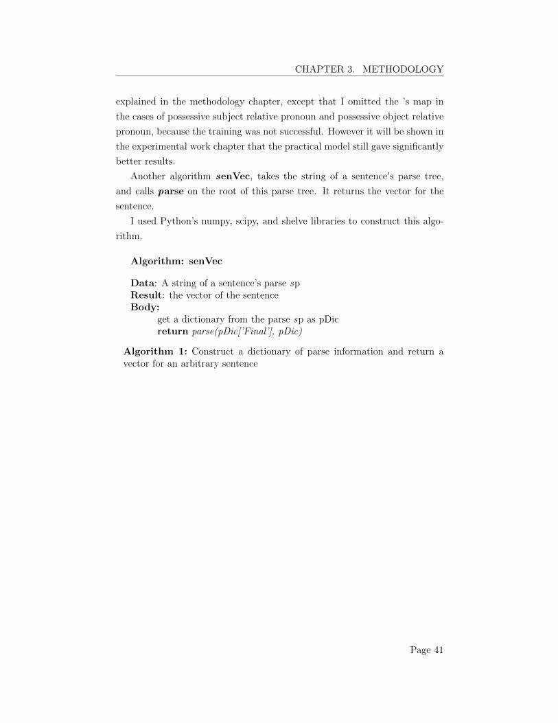
The algorithm parse takes in a sentence’s parse information, and a string
of the parse of current node, denoted by the notation in the previous section,
returns a vector. It assumes that a word semantic vector space and relational
words’ tensor spaces are ready to use. The body of this algorithm first looks
at the input string, which is the compositional information of current level
in a parse tree. For example, A=river#n+canal#n+lake#n in the previous
example, or the root Final=ground#n|near#p|B. If it is a single word, then
the algorithm returns a vector or a tensor according to its type; if it is a
phrase, the algorithm will first determine which kind of phrase it is, then call
itself recursively to return a proper vector. The algorithm follows the models
Page 40
CHAPTER 3. METHODOLOGY
explained in the methodology chapter, except that I omitted the ’s map in
the cases of possessive subject relative pronoun and possessive object relative
pronoun, because the training was not successful. However it will be shown in
the experimental work chapter that the practical model still gave significantly
better results.
Another algorithm senVec, takes the string of a sentence’s parse tree,
and calls parse on the root of this parse tree. It returns the vector for the
sentence.
I used Python’s numpy, scipy, and shelve libraries to construct this algo-
rithm.
Algorithm: senVec
Data: A string of a sentence’s parse spResult: the vector of the sentenceBody:
get a dictionary from the parse sp as pDicreturn parse(pDic[’Final’], pDic)
Algorithm 1: Construct a dictionary of parse information and return avector for an arbitrary sentence
Page 41
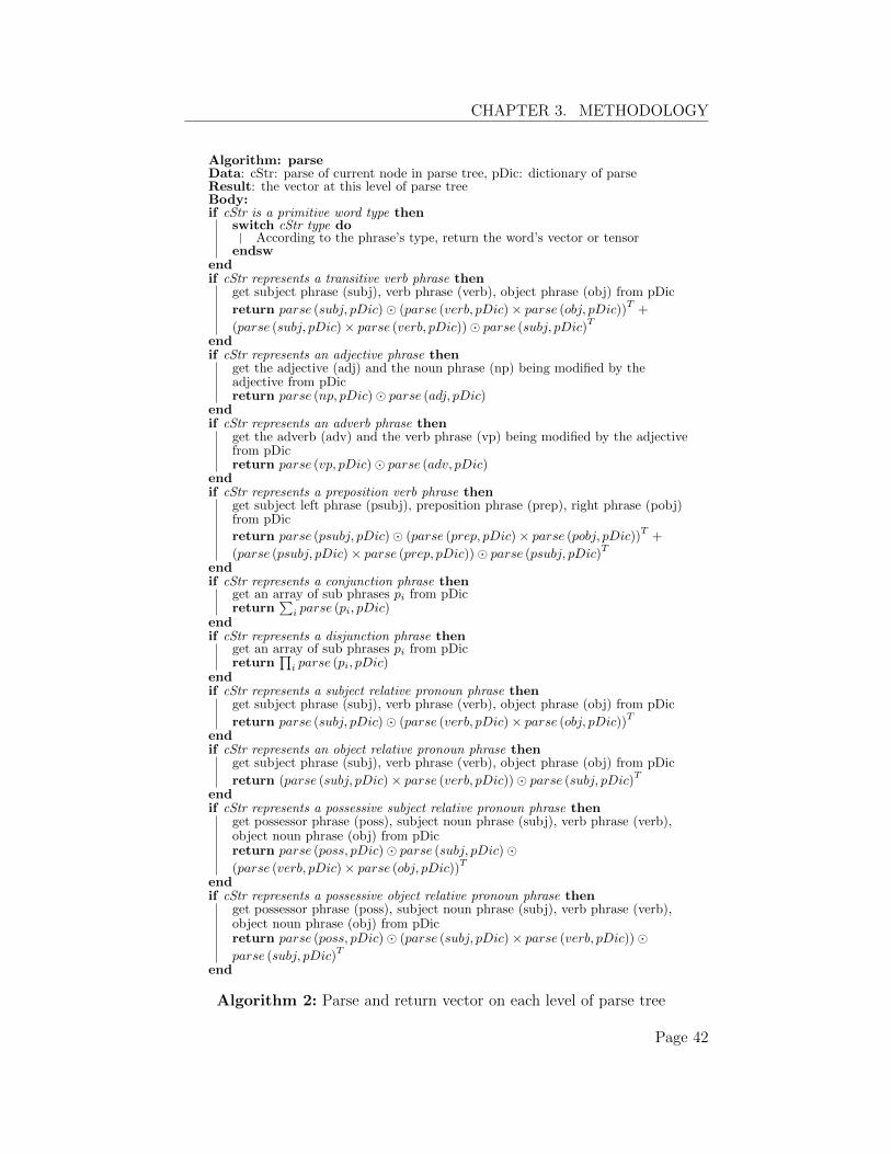
CHAPTER 3. METHODOLOGY
Algorithm: parse
Data: cStr: parse of current node in parse tree, pDic: dictionary of parseResult: the vector at this level of parse treeBody:
if cStr is a primitive word type then
switch cStr type do
According to the phrase’s type, return the word’s vector or tensorendsw
end
if cStr represents a transitive verb phrase then
get subject phrase (subj), verb phrase (verb), object phrase (obj) from pDic
return parse (subj, pDic)� (parse (verb, pDic)⇥ parse (obj, pDic))T+
(parse (subj, pDic)⇥ parse (verb, pDic))� parse (subj, pDic)T
end
if cStr represents an adjective phrase then
get the adjective (adj) and the noun phrase (np) being modified by theadjective from pDicreturn parse (np, pDic)� parse (adj, pDic)
end
if cStr represents an adverb phrase then
get the adverb (adv) and the verb phrase (vp) being modified by the adjectivefrom pDicreturn parse (vp, pDic)� parse (adv, pDic)
end
if cStr represents a preposition verb phrase then
get subject left phrase (psubj), preposition phrase (prep), right phrase (pobj)from pDic
return parse (psubj, pDic)� (parse (prep, pDic)⇥ parse (pobj, pDic))T+
(parse (psubj, pDic)⇥ parse (prep, pDic))� parse (psubj, pDic)T
end
if cStr represents a conjunction phrase then
get an array of sub phrases pi from pDicreturn
Pi parse (pi, pDic)
end
if cStr represents a disjunction phrase then
get an array of sub phrases pi from pDicreturn
Qi parse (pi, pDic)
end
if cStr represents a subject relative pronoun phrase then
get subject phrase (subj), verb phrase (verb), object phrase (obj) from pDic
return parse (subj, pDic)� (parse (verb, pDic)⇥ parse (obj, pDic))T
end
if cStr represents an object relative pronoun phrase then
get subject phrase (subj), verb phrase (verb), object phrase (obj) from pDic
return (parse (subj, pDic)⇥ parse (verb, pDic))� parse (subj, pDic)T
end
if cStr represents a possessive subject relative pronoun phrase then
get possessor phrase (poss), subject noun phrase (subj), verb phrase (verb),object noun phrase (obj) from pDicreturn parse (poss, pDic)� parse (subj, pDic)�(parse (verb, pDic)⇥ parse (obj, pDic))
T
end
if cStr represents a possessive object relative pronoun phrase then
get possessor phrase (poss), subject noun phrase (subj), verb phrase (verb),object noun phrase (obj) from pDicreturn parse (poss, pDic)� (parse (subj, pDic)⇥ parse (verb, pDic))�parse (subj, pDic)
T
end
Algorithm 2: Parse and return vector on each level of parse tree
Page 42
Chapter 4
Experimental work
4.1 A term-definition classification task
The experimental work of this research is based on a term-definition classi-
fication task first introduced by Kartsaklis et al. [19] to match terms with
phrases. In their paper 112 terms from the Oxford Junior Dictionary were
extracted. Each term in the dataset contains three definitions from the Ox-
ford Junior Dictionary itself [32], the Oxford Concise School Dictionary, and
the WordNet [19]. The task was to treat terms as classes, and use cosine dis-
tance as similarity. Finally, a definition is assigned to the term which is most
similar (smallest cosine distance). The results were evaluated by calculating
the accuracy of the classification task. Nouns and verbs with very simple
definitions were evaluated in their experiment, and the categorical model was
scored slightly higher than the baseline models.
In this experiment, I used the mean reciprocal rank (MRR) in addition to
accuracy. MRR gives more objective results, it considers “how good” the vec-
tors are instead of just looking at how many definitions are matched exactly.
This experiment involves larger datasets, therefore MRR is necessary to give
a good idea for each model’s overall performance.
4.2 Extract datasets for evaluation
In this experiment, I extracted data only from the Oxford Junior Dictionary,
and all terms are nouns; therefore all definitions are noun phrases. There
are thousands of words in the dictionary; each word contains at least one
43
CHAPTER 4. EXPERIMENTAL WORK
definition. I used a collection of 221 nouns’ term-definition pairs randomly
extracted from the dictionary, and each term only keeps one definition. I
classified the definition phrases into two types: non-recursive phrases and
recursive phrases as introduced in section 3.4.9.
Examples of non-recursive phrases are “a particular thing” and “woman
who rules a country”. They are non-recursive because “a particular thing” is
a direct composition of an adjective “particular” and a noun “thing”, where
“particular” is an adjective that expects one argument on its right; and
“woman who rules a country” is a direct composition of “woman”, “rules”
and “country”, where “rules” is a transitive verb that expects two arguments.
Examples of recursive phrases are “a lot of loud noise” and “a big party with
a lot of dancing”. The first phrase has “loud noise” and then “a lot of loud
noise”; the second phrase has “a big party”, “a lot of dancing”, and the two
parts get composed as “a big party with a lot of dancing”.
There are 104 term-definition pairs containing non-recursive (simple) phrases
and 77 term-definition pairs containing recursive (complex) phrases. Some
additional term-definition pairs are added to this dataset to create a unified
evaluation at the end.
I also created datasets for a few specific cases in order to evaluate the
categorical model on di↵erent types of relational words under the current
experimental setting. Specifically, subject/object relative pronoun phrases,
preposition phrases, transitive verb phrases and adjective phrases. They are
mostly simple (non-recursive) phrases. There are not enough non-recursive
phrases for disjunctions, conjunctions and adverbs to extract from the dictio-
nary dataset I obtained; therefore the specific evaluation on these three types
of words is not performed in this experiment.
The datasets are available in the Appendix.
4.3 Baseline evaluation methods
This section introduces the baseline methods of creating vectors for phrases
and sentences: the additive model, the multiplicative model, and a head word
model.
Page 44
CHAPTER 4. EXPERIMENTAL WORK
4.3.1 An additive model
In the additive model, a sentence vector is created by adding all the order-1
word vectors from the sentence. In practice, the additive model can add all
word vectors in a sentence. However, because of the stop words (very frequent
words) and some insignificant words (words not contributing to the meaning
of a sentence, such as prepositions, logical words, etc.), adding all words might
not give good results. The reason is that stop words occur so frequently that
they can be with any other words. For example, “very”, “is”, and “of” can
appear everywhere in an article. Their vectors will have similar numbers for
each entry element, which means the they will not contribute much about the
meaning of a sentence overall. Instead, adding these vectors could reduce the
accuracy of the sentence vector produced.
In the actual experiment I conducted, the sentence was first preprocessed
to remove all stop words and insignificant words (such as determinators). The
model then adds the rest words’ vectors to produce a sentence vector.
4.3.2 A multiplicative model
In the multiplicative model, a sentence vector is created by point-wise mul-
tiplying all the order-1 word vectors in the sentence. Again in practice, the
multiplicative model can point-wise multiply all word vectors in a sentence.
However, the stop words and insignificant words will not contribute to the sen-
tence vector positively. In the actual experiment, stop words and insignificant
words were dropped.
4.3.3 Head word of sentence
In some cases, the head word of a sentence is most significant and could
stand in a position that best represents a sentence. One good example is a
the term-definition pair, “coach” and “bus that takes people”, where “bus” is
already very close to “coach”. This is obviously not always true. For example,
consider the term-definition pair, “clerk” and “someone who writes letters”.
The word “someone” in some case would not be a good representative for the
term “clerk”. The head word model surely does not capture all the important
information of the sentence. However, this method is nevertheless a trivial
baseline method.
Page 45
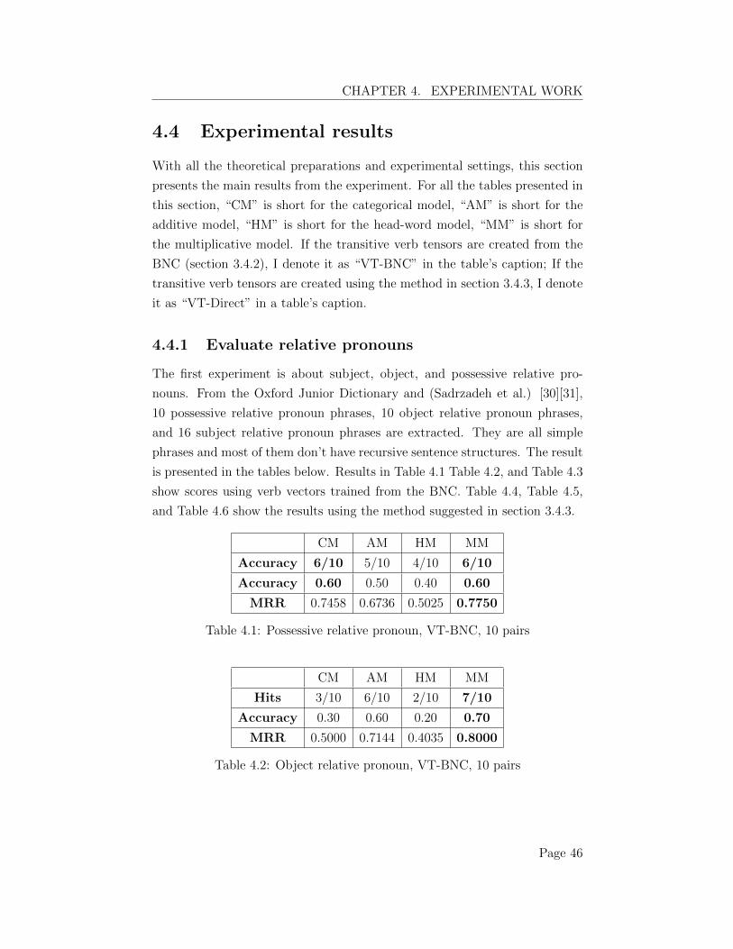
CHAPTER 4. EXPERIMENTAL WORK
4.4 Experimental results
With all the theoretical preparations and experimental settings, this section
presents the main results from the experiment. For all the tables presented in
this section, “CM” is short for the categorical model, “AM” is short for the
additive model, “HM” is short for the head-word model, “MM” is short for
the multiplicative model. If the transitive verb tensors are created from the
BNC (section 3.4.2), I denote it as “VT-BNC” in the table’s caption; If the
transitive verb tensors are created using the method in section 3.4.3, I denote
it as “VT-Direct” in a table’s caption.
4.4.1 Evaluate relative pronouns
The first experiment is about subject, object, and possessive relative pro-
nouns. From the Oxford Junior Dictionary and (Sadrzadeh et al.) [30][31],
10 possessive relative pronoun phrases, 10 object relative pronoun phrases,
and 16 subject relative pronoun phrases are extracted. They are all simple
phrases and most of them don’t have recursive sentence structures. The result
is presented in the tables below. Results in Table 4.1 Table 4.2, and Table 4.3
show scores using verb vectors trained from the BNC. Table 4.4, Table 4.5,
and Table 4.6 show the results using the method suggested in section 3.4.3.
CM AM HM MM
Accuracy 6/10 5/10 4/10 6/10
Accuracy 0.60 0.50 0.40 0.60
MRR 0.7458 0.6736 0.5025 0.7750
Table 4.1: Possessive relative pronoun, VT-BNC, 10 pairs
CM AM HM MM
Hits 3/10 6/10 2/10 7/10
Accuracy 0.30 0.60 0.20 0.70
MRR 0.5000 0.7144 0.4035 0.8000
Table 4.2: Object relative pronoun, VT-BNC, 10 pairs
Page 46
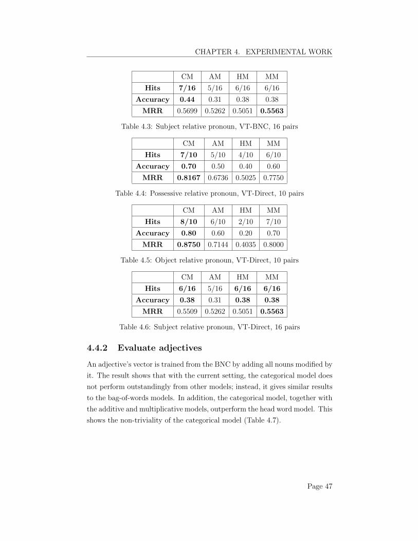
CHAPTER 4. EXPERIMENTAL WORK
CM AM HM MM
Hits 7/16 5/16 6/16 6/16
Accuracy 0.44 0.31 0.38 0.38
MRR 0.5699 0.5262 0.5051 0.5563
Table 4.3: Subject relative pronoun, VT-BNC, 16 pairs
CM AM HM MM
Hits 7/10 5/10 4/10 6/10
Accuracy 0.70 0.50 0.40 0.60
MRR 0.8167 0.6736 0.5025 0.7750
Table 4.4: Possessive relative pronoun, VT-Direct, 10 pairs
CM AM HM MM
Hits 8/10 6/10 2/10 7/10
Accuracy 0.80 0.60 0.20 0.70
MRR 0.8750 0.7144 0.4035 0.8000
Table 4.5: Object relative pronoun, VT-Direct, 10 pairs
CM AM HM MM
Hits 6/16 5/16 6/16 6/16
Accuracy 0.38 0.31 0.38 0.38
MRR 0.5509 0.5262 0.5051 0.5563
Table 4.6: Subject relative pronoun, VT-Direct, 16 pairs
4.4.2 Evaluate adjectives
An adjective’s vector is trained from the BNC by adding all nouns modified by
it. The result shows that with the current setting, the categorical model does
not perform outstandingly from other models; instead, it gives similar results
to the bag-of-words models. In addition, the categorical model, together with
the additive and multiplicative models, outperform the head word model. This
shows the non-triviality of the categorical model (Table 4.7).
Page 47
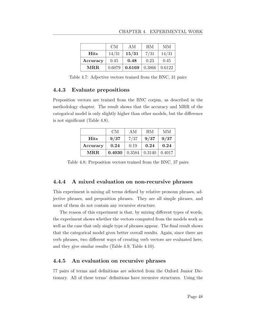
CHAPTER 4. EXPERIMENTAL WORK
CM AM HM MM
Hits 14/31 15/31 7/31 14/31
Accuracy 0.45 0.48 0.23 0.45
MRR 0.6079 0.6169 0.3866 0.6122
Table 4.7: Adjective vectors trained from the BNC, 31 pairs
4.4.3 Evaluate prepositions
Preposition vectors are trained from the BNC corpus, as described in the
methodology chapter. The result shows that the accuracy and MRR of the
categorical model is only slightly higher than other models, but the di↵erence
is not significant (Table 4.8).
CM AM HM MM
Hits 9/37 7/37 9/37 9/37
Accuracy 0.24 0.19 0.24 0.24
MRR 0.4030 0.3584 0.3140 0.4017
Table 4.8: Preposition vectors trained from the BNC, 37 pairs
4.4.4 A mixed evaluation on non-recursive phrases
This experiment is mixing all terms defined by relative pronoun phrases, ad-
jective phrases, and preposition phrases. They are all simple phrases, and
most of them do not contain any recursive structure.
The reason of this experiment is that, by mixing di↵erent types of words,
the experiment shows whether the vectors computed from the models work as
well as the case that only single type of phrases appear. The final result shows
that the categorical model gives better overall results. Again, since there are
verb phrases, two di↵erent ways of creating verb vectors are evaluated here,
and they give similar results (Table 4.9, Table 4.10).
4.4.5 An evaluation on recursive phrases
77 pairs of terms and definitions are selected from the Oxford Junior Dic-
tionary. All of these terms’ definitions have recursive structures. Using the
Page 48
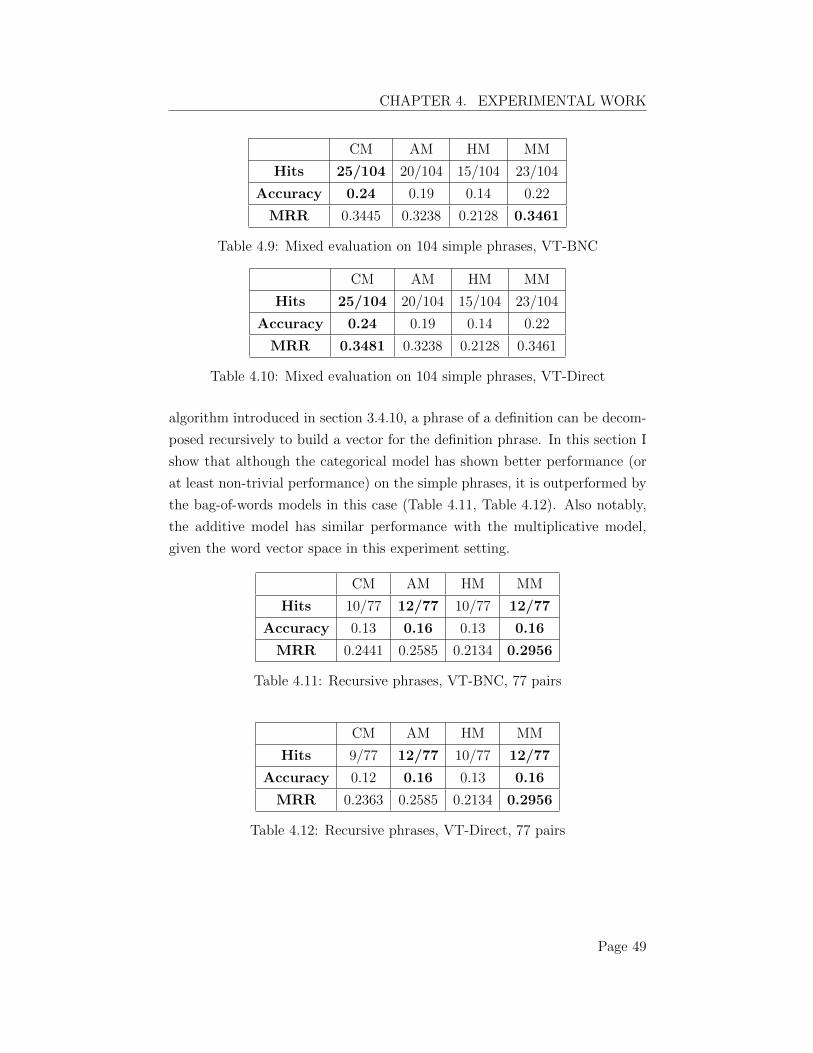
CHAPTER 4. EXPERIMENTAL WORK
CM AM HM MM
Hits 25/104 20/104 15/104 23/104
Accuracy 0.24 0.19 0.14 0.22
MRR 0.3445 0.3238 0.2128 0.3461
Table 4.9: Mixed evaluation on 104 simple phrases, VT-BNC
CM AM HM MM
Hits 25/104 20/104 15/104 23/104
Accuracy 0.24 0.19 0.14 0.22
MRR 0.3481 0.3238 0.2128 0.3461
Table 4.10: Mixed evaluation on 104 simple phrases, VT-Direct
algorithm introduced in section 3.4.10, a phrase of a definition can be decom-
posed recursively to build a vector for the definition phrase. In this section I
show that although the categorical model has shown better performance (or
at least non-trivial performance) on the simple phrases, it is outperformed by
the bag-of-words models in this case (Table 4.11, Table 4.12). Also notably,
the additive model has similar performance with the multiplicative model,
given the word vector space in this experiment setting.
CM AM HM MM
Hits 10/77 12/77 10/77 12/77
Accuracy 0.13 0.16 0.13 0.16
MRR 0.2441 0.2585 0.2134 0.2956
Table 4.11: Recursive phrases, VT-BNC, 77 pairs
CM AM HM MM
Hits 9/77 12/77 10/77 12/77
Accuracy 0.12 0.16 0.13 0.16
MRR 0.2363 0.2585 0.2134 0.2956
Table 4.12: Recursive phrases, VT-Direct, 77 pairs
Page 49
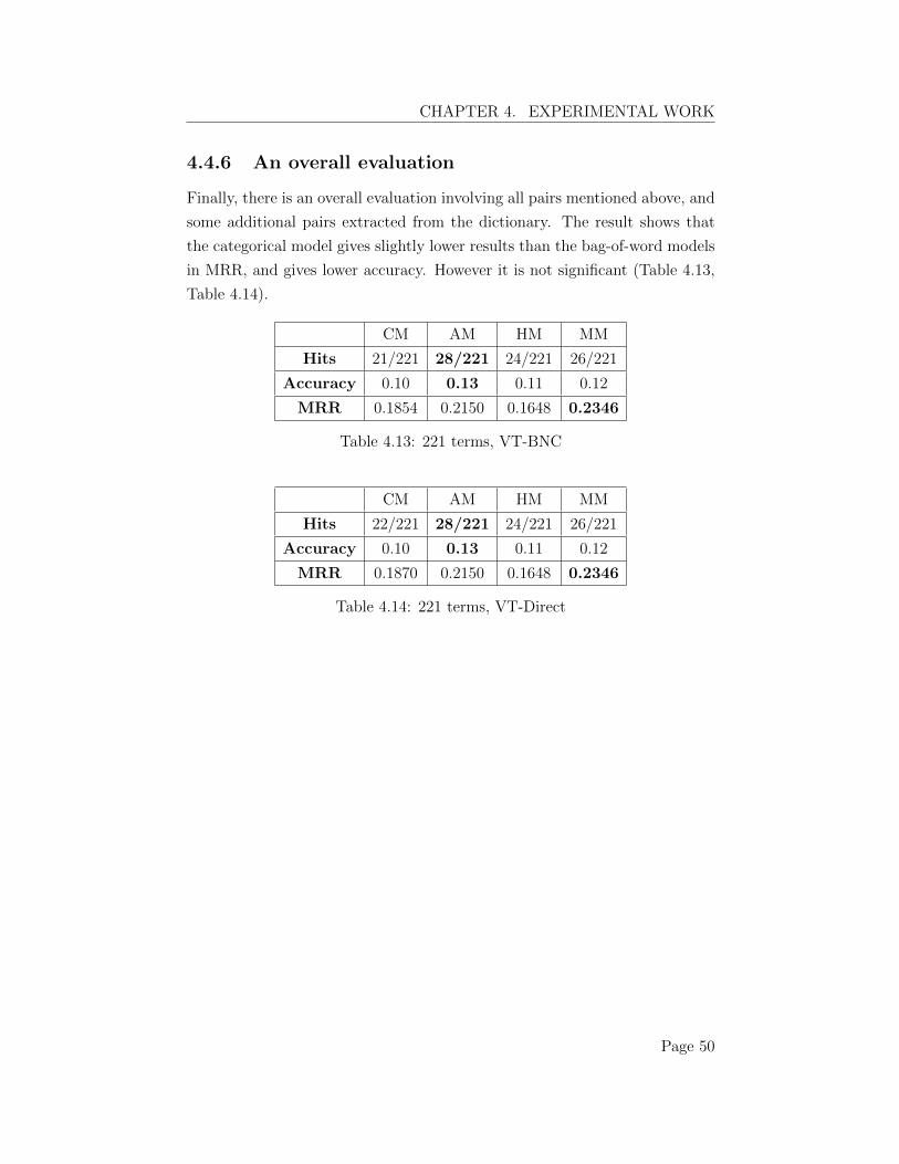
CHAPTER 4. EXPERIMENTAL WORK
4.4.6 An overall evaluation
Finally, there is an overall evaluation involving all pairs mentioned above, and
some additional pairs extracted from the dictionary. The result shows that
the categorical model gives slightly lower results than the bag-of-word models
in MRR, and gives lower accuracy. However it is not significant (Table 4.13,
Table 4.14).
CM AM HM MM
Hits 21/221 28/221 24/221 26/221
Accuracy 0.10 0.13 0.11 0.12
MRR 0.1854 0.2150 0.1648 0.2346
Table 4.13: 221 terms, VT-BNC
CM AM HM MM
Hits 22/221 28/221 24/221 26/221
Accuracy 0.10 0.13 0.11 0.12
MRR 0.1870 0.2150 0.1648 0.2346
Table 4.14: 221 terms, VT-Direct
Page 50

Chapter 5
Discussion
5.1 Overall performance of the categorical model
The primary objective of this research is to give a unified evaluation for the
categorical compositional-distributional model. With the current experimen-
tal setting, there are a few observations:
1. The categorical model is non-trivial: the results show that the cate-
gorical model outperforms the head-word baseline. This is as expected
because the head-word baseline model is only a vague and sometimes in-
accurate approximation to the meaning of a whole phrase. It is expected
that the categorical model, the additive model, and the multiplicative
model give better results, because they take more information into ac-
count from a phrase.
2. The categorical model gives better performance on non-recursive phrases
(i.e. simple phrases). I expected that the categorical model gives better
results than any other bag-of-words baseline models because the cat-
egorical model not only considers individual words’ meaning, but also
considers the compositional information in the phrase. It treats rela-
tional words as multi-linear maps and compose the vectors in a mean-
ingful way. The experiment also shows that the categorical model does
not give significantly better results (rather, it is just a bit better than
the additive model and the multiplicative model). I suspect that this
is because of the simplification during the training of relational words’
vectors: I used the Frobenius algebra operation � to expand a vector
51
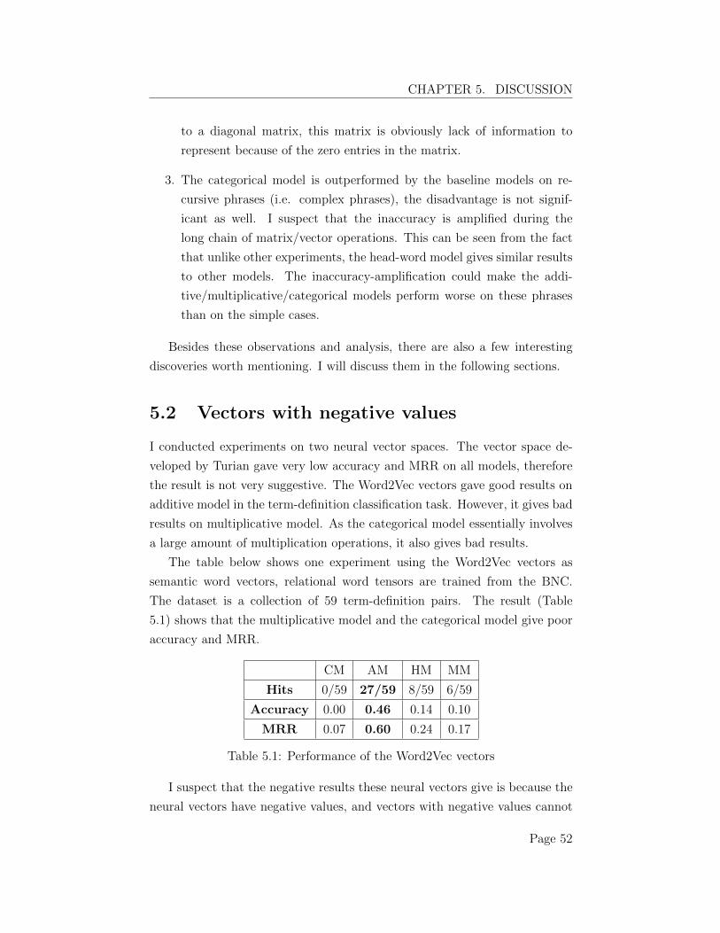
CHAPTER 5. DISCUSSION
to a diagonal matrix, this matrix is obviously lack of information to
represent because of the zero entries in the matrix.
3. The categorical model is outperformed by the baseline models on re-
cursive phrases (i.e. complex phrases), the disadvantage is not signif-
icant as well. I suspect that the inaccuracy is amplified during the
long chain of matrix/vector operations. This can be seen from the fact
that unlike other experiments, the head-word model gives similar results
to other models. The inaccuracy-amplification could make the addi-
tive/multiplicative/categorical models perform worse on these phrases
than on the simple cases.
Besides these observations and analysis, there are also a few interesting
discoveries worth mentioning. I will discuss them in the following sections.
5.2 Vectors with negative values
I conducted experiments on two neural vector spaces. The vector space de-
veloped by Turian gave very low accuracy and MRR on all models, therefore
the result is not very suggestive. The Word2Vec vectors gave good results on
additive model in the term-definition classification task. However, it gives bad
results on multiplicative model. As the categorical model essentially involves
a large amount of multiplication operations, it also gives bad results.
The table below shows one experiment using the Word2Vec vectors as
semantic word vectors, relational word tensors are trained from the BNC.
The dataset is a collection of 59 term-definition pairs. The result (Table
5.1) shows that the multiplicative model and the categorical model give poor
accuracy and MRR.
CM AM HM MM
Hits 0/59 27/59 8/59 6/59
Accuracy 0.00 0.46 0.14 0.10
MRR 0.07 0.60 0.24 0.17
Table 5.1: Performance of the Word2Vec vectors
I suspect that the negative results these neural vectors give is because the
neural vectors have negative values, and vectors with negative values cannot
Page 52
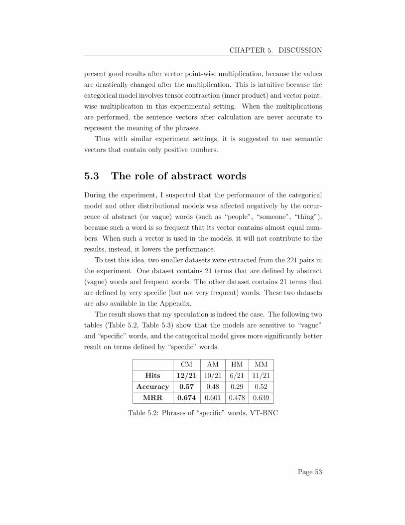
CHAPTER 5. DISCUSSION
present good results after vector point-wise multiplication, because the values
are drastically changed after the multiplication. This is intuitive because the
categorical model involves tensor contraction (inner product) and vector point-
wise multiplication in this experimental setting. When the multiplications
are performed, the sentence vectors after calculation are never accurate to
represent the meaning of the phrases.
Thus with similar experiment settings, it is suggested to use semantic
vectors that contain only positive numbers.
5.3 The role of abstract words
During the experiment, I suspected that the performance of the categorical
model and other distributional models was a↵ected negatively by the occur-
rence of abstract (or vague) words (such as “people”, “someone”, “thing”),
because such a word is so frequent that its vector contains almost equal num-
bers. When such a vector is used in the models, it will not contribute to the
results, instead, it lowers the performance.
To test this idea, two smaller datasets were extracted from the 221 pairs in
the experiment. One dataset contains 21 terms that are defined by abstract
(vague) words and frequent words. The other dataset contains 21 terms that
are defined by very specific (but not very frequent) words. These two datasets
are also available in the Appendix.
The result shows that my speculation is indeed the case. The following two
tables (Table 5.2, Table 5.3) show that the models are sensitive to “vague”
and “specific” words, and the categorical model gives more significantly better
result on terms defined by “specific” words.
CM AM HM MM
Hits 12/21 10/21 6/21 11/21
Accuracy 0.57 0.48 0.29 0.52
MRR 0.674 0.601 0.478 0.639
Table 5.2: Phrases of “specific” words, VT-BNC
Page 53
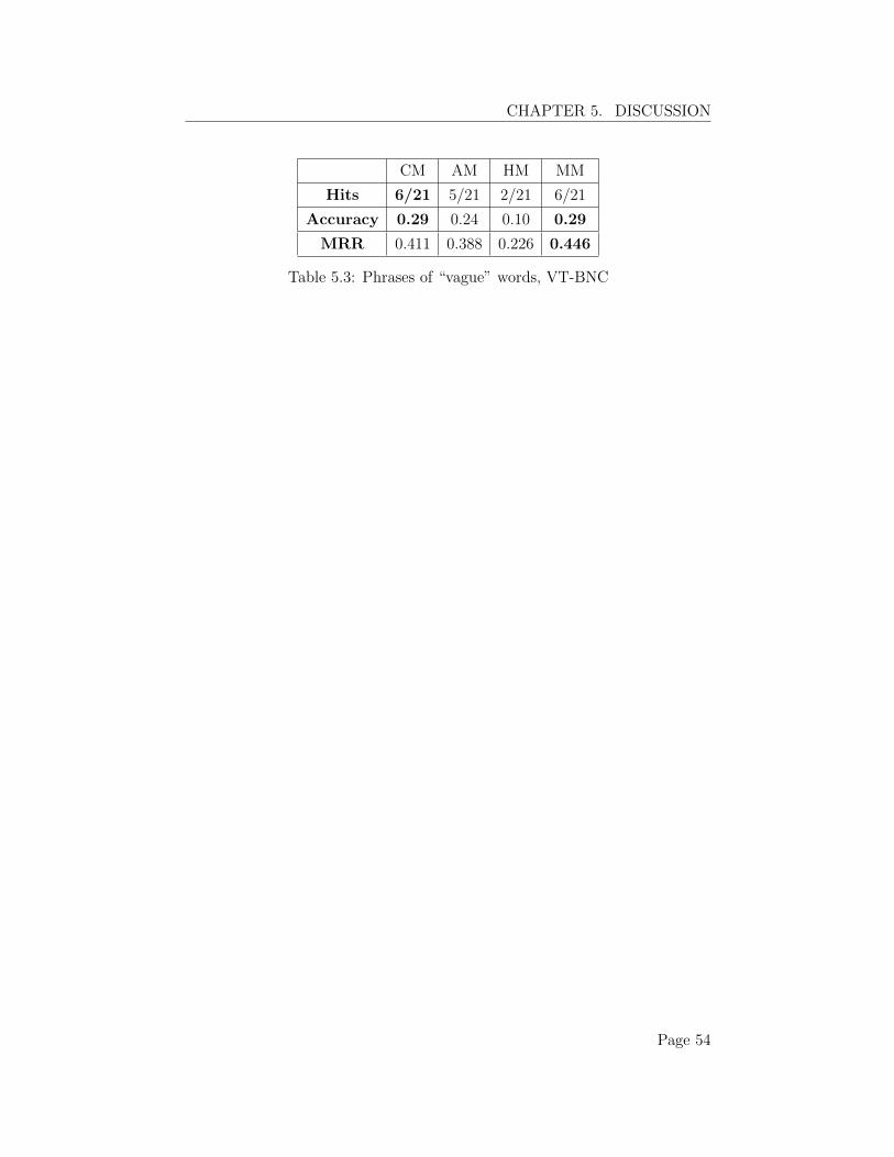
CHAPTER 5. DISCUSSION
CM AM HM MM
Hits 6/21 5/21 2/21 6/21
Accuracy 0.29 0.24 0.10 0.29
MRR 0.411 0.388 0.226 0.446
Table 5.3: Phrases of “vague” words, VT-BNC
Page 54
Chapter 6
Future work
6.1 Further investigation into phrases of “vague”
and “specific” words
One immediate task that could be done is to expand datasets of phrases of
“vague” words and phrases of “specific” words. A large scale evaluation of
this could help the understanding of the performance of distributional models
over di↵erent types of words, and especially how the categorical model reacts
on the di↵erence.
6.2 Negative phrases
Negative phrases and sentences are not discussed in this work. However nega-
tive phrases are not unusual. (Coecke et al.) [6] has already modeled negative
sentences within the categorical framework. An e↵ective way of evaluating
how the categorical model performs on negative phrases and sentences is nec-
essary.
6.3 Reduce size of semantic word vector space
As stated previously, under the experimental setting of this project, only vec-
tor spaces containing positive numbers can be used because they work on
multiplication and inner product. The vector is 2000-dimension, taking more
than 5Gb space on disk (as a shelve database). When training relational
55
CHAPTER 6. FUTURE WORK
word vectors, a matrix for one relational word can take up to 1Gb space on
disk. Even for evaluation task, this is over sized. Any attempt to reduce the
size of semantic word space is plausible. One possible attempt is to perform
non-negative matrix factorization on the vector space to produce a word vec-
tor space of lower dimensionality while preserving its performance on word
similarity comparison.
6.4 Other ways of training relational word vec-
tors
The relational words’ representations are created using a tensor based ap-
proach in this project, and the tensors are created directly from the BNC
corpus. However, this approach only creates tensors that are 1-order less than
it should be. For example, an adjective’s vector is created by adding all nouns’
vectors modified by the adjective in the corpus. The result is a order-1 vector
instead of a matrix. The Frobenius algebra copy operation creates a diagonal
matrix, which might not contain enough information for how the adjective is
modifying other nouns. Same for a transitive verb, the outcome is a matrix
instead of a “cube”, hence Frobenius algebra copy operation is used to expand
it to a cube. However the cube only has non-zero numbers on its diagonal
plane, which again might not be a complete representation of a transitive verb.
However, the tensor-based approach in the experiment cannot create a
adjective matrix or a transitive verb “cube” easily, because there is no infor-
mation to represent the extra order. Some machine learning techniques can
be used to create complete “matrices” and “cubes”.
Page 56
Chapter 7
Conclusion
A practical categorical model was instantiated on concrete distributional mod-
els in this research. It could compute vectors for complex sentences and
phrases based on the categorical model of sentence meaning. A dataset for
large-scale evaluation was extracted from the Oxford Junior Dictionary. Based
on the practical model and the evaluation dataset, a large scale, generic eval-
uation was performed. The experimental results has been giving valuable
insights into the practice of building distributional models and especially,
building categorical models. Future practical models and experiments can
be set up based on this work.
57
Bibliography
[1] J. Barwise and R. Cooper. Generalized quantifiers and natural language.
Linguistics and philosophy, 4(2):159–219, 1981.
[2] N. Chomsky. Syntactic structures. Walter de Gruyter, 2002.
[3] S. Clark and S. Pulman. Combining symbolic and distributional models
of meaning. In AAAI Spring Symposium: Quantum Interaction, pages
52–55, 2007.
[4] B. Coecke. Quantum picturalism. Contemporary physics, 51(1):59–83,
2010.
[5] B. Coecke and E. O. Paquette. Categories for the practising physicist.
In New Structures for Physics, pages 173–286. Springer, 2011.
[6] B. Coecke, M. Sadrzadeh, and S. Clark. Mathematical foundations
for a compositional distributional model of meaning. arXiv preprint
arXiv:1003.4394, 2010.
[7] R. Collobert and J. Weston. A unified architecture for natural language
processing: Deep neural networks with multitask learning. In Proceedings
of the 25th international conference on Machine learning, pages 160–167.
ACM, 2008.
[8] J. R. Curran, S. Clark, and J. Bos. Linguistically motivated large-scale
nlp with c&c and boxer. In Proceedings of the 45th Annual Meeting of
the ACL on Interactive Poster and Demonstration Sessions, pages 33–36.
Association for Computational Linguistics, 2007.
[9] D. R. Dowty. Word meaning and Montague grammar: The semantics
of verbs and times in generative semantics and in Montague’s PTQ, vol-
ume 7. Springer, 1979.
58
BIBLIOGRAPHY
[10] A. Ferraresi, E. Zanchetta, M. Baroni, and S. Bernardini. Introducing
and evaluating ukwac, a very large web-derived corpus of english. In
Proceedings of the 4th Web as Corpus Workshop (WAC-4) Can we beat
Google, pages 47–54, 2008.
[11] G. Frege. The Foundations of Arithmetic: A logico-mathematical enquiry
into the concept of number. Northwestern University Press, 1980.
[12] G. Frege. Ueber sinn und bedeutunq (on sense and reference). Per-
spectives in the Philosophy of Language: A Concise Anthology, page 45,
2000.
[13] R. Ge and R. J. Mooney. A statistical semantic parser that integrates
syntax and semantics. In Proceedings of the Ninth Conference on Com-
putational Natural Language Learning, pages 9–16. Association for Com-
putational Linguistics, 2005.
[14] D. Gra↵, J. Kong, K. Chen, and K. Maeda. English gigaword. Linguistic
Data Consortium, Philadelphia, 2003.
[15] E. Grefenstette. Category-theoretic quantitative compositional dis-
tributional models of natural language semantics. arXiv preprint
arXiv:1311.1539, 2013.
[16] E. Grefenstette and M. Sadrzadeh. Experimental support for a categorical
compositional distributional model of meaning. In Proceedings of the
Conference on Empirical Methods in Natural Language Processing, pages
1394–1404. Association for Computational Linguistics, 2011.
[17] D. Kartsaklis. Compositional operators in distributional semantics. arXiv
preprint arXiv:1401.5327, 2014.
[18] D. Kartsaklis, N. Kalchbrenner, and M. Sadrzadeh. Resolving lexical
ambiguity in tensor regression models of meaning. In Proceedings of the
52th Annual Meeting of the Association for Computational Linguistics
(ACL): Short Papers, Baltimore, USA. To appear, 2014.
[19] D. Kartsaklis, M. Sadrzadeh, and S. Pulman. A unified sentence space
for categorical distributional-compositional semantics: Theory and ex-
periments. In In Proceedings of COLING: Posters. Citeseer, 2012.
Page 59
BIBLIOGRAPHY
[20] J. Lambek. Type grammars as pregroups. Grammars, 4(1):21–39, 2001.
[21] J. Lambek. From Word to Sentence: a computational algebraic approach
to grammar. Polimetrica sas, 2008.
[22] J. Lambek. Pregroup grammars and chomsky’s earliest examples. Journal
of Logic, Language and Information, 17(2):141–160, 2008.
[23] T. Mikolov, K. Chen, G. Corrado, and J. Dean. E�cient estimation of
word representations in vector space. arXiv preprint arXiv:1301.3781,
2013.
[24] J. Mitchell and M. Lapata. Composition in distributional models of se-
mantics. Cognitive science, 34(8):1388–1429, 2010.
[25] D. K. Modrak. Aristotle’s theory of language and meaning. Cambridge
University Press, 2001.
[26] R. Montague. Universal grammar. Theoria, 36(3):373–398, 1970.
[27] B. C. Pierce. Basic category theory for computer scientists. MIT press,
1991.
[28] H. Rubenstein and J. B. Goodenough. Contextual correlates of synonymy.
Communications of the ACM, 8(10):627–633, 1965.
[29] V. Rus, P. M. McCarthy, M. C. Lintean, D. S. McNamara, and A. C.
Graesser. Paraphrase identification with lexico-syntactic graph subsump-
tion. In FLAIRS conference, pages 201–206, 2008.
[30] M. Sadrzadeh, S. Clark, and B. Coecke. The frobenius anatomy of word
meanings i: subject and object relative pronouns. Journal of Logic and
Computation, 23(6):1293–1317, 2013.
[31] M. Sadrzadeh, S. Clark, and B. Coecke. The frobenius anatomy of word
meanings ii: possessive relative pronouns. Journal of Logic and Compu-
tation, page exu027, 2014.
[32] R. Sansome, D. Reid, A. Spooner, and B. Rowe. The Oxford Illustrated
Junior Dictionary. Oxford University Press, 2000.
Page 60
BIBLIOGRAPHY
[33] R. Socher, E. H. Huang, J. Pennington, A. Y. Ng, and C. D. Manning.
Dynamic pooling and unfolding recursive autoencoders for paraphrase
detection. In NIPS, volume 24, pages 801–809, 2011.
[34] R. Socher, B. Huval, C. D. Manning, and A. Y. Ng. Semantic compo-
sitionality through recursive matrix-vector spaces. In Proceedings of the
2012 Joint Conference on Empirical Methods in Natural Language Pro-
cessing and Computational Natural Language Learning, pages 1201–1211.
Association for Computational Linguistics, 2012.
[35] R. Socher, C. C. Lin, C. Manning, and A. Y. Ng. Parsing natural scenes
and natural language with recursive neural networks. In Proceedings
of the 28th International Conference on Machine Learning (ICML-11),
pages 129–136, 2011.
[36] R. Socher, C. D. Manning, and A. Y. Ng. Learning continuous phrase
representations and syntactic parsing with recursive neural networks. In
Proceedings of the NIPS-2010 Deep Learning and Unsupervised Feature
Learning Workshop, pages 1–9, 2010.
[37] R. Socher, J. Pennington, E. H. Huang, A. Y. Ng, and C. D. Manning.
Semi-supervised recursive autoencoders for predicting sentiment distribu-
tions. In Proceedings of the Conference on Empirical Methods in Natural
Language Processing, pages 151–161. Association for Computational Lin-
guistics, 2011.
[38] J. Turian, L. Ratinov, and Y. Bengio. Word representations: a simple
and general method for semi-supervised learning. In Proceedings of the
48th Annual Meeting of the Association for Computational Linguistics,
pages 384–394. Association for Computational Linguistics, 2010.
[39] S. Wan, M. Dras, R. Dale, and C. Paris. Using dependency-based fea-
tures to take the “para-farce” out of paraphrase. In Proceedings of the
Australasian Language Technology Workshop, volume 2006, 2006.
[40] L. Wittgenstein. Philosophical investigations. John Wiley & Sons, 2010.
[41] L. S. Zettlemoyer and M. Collins. Learning to map sentences to logical
form: Structured classification with probabilistic categorial grammars.
arXiv preprint arXiv:1207.1420, 2012.
Page 61
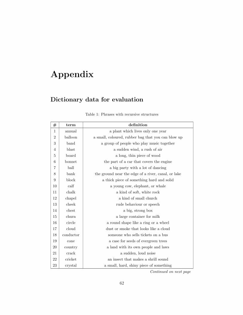
Appendix
Dictionary data for evaluation
Table 1: Phrases with recursive structures
# term definition
1 annual a plant which lives only one year
2 balloon a small, coloured, rubber bag that you can blow up
3 band a group of people who play music together
4 blast a sudden wind, a rush of air
5 board a long, thin piece of wood
6 bonnet the part of a car that covers the engine
7 ball a big party with a lot of dancing
8 bank the ground near the edge of a river, canal, or lake
9 block a thick piece of something hard and solid
10 calf a young cow, elephant, or whale
11 chalk a kind of soft, white rock
12 chapel a kind of small church
13 cheek rude behaviour or speech
14 chest a big, strong box
15 churn a large container for milk
16 circle a round shape like a ring or a wheel
17 cloud dust or smoke that looks like a cloud
18 conductor someone who sells tickets on a bus
19 cone a case for seeds of evergreen trees
20 country a land with its own people and laws
21 crack a sudden, loud noise
22 cricket an insect that makes a shrill sound
23 crystal a small, hard, shiny piece of something
Continued on next page
62
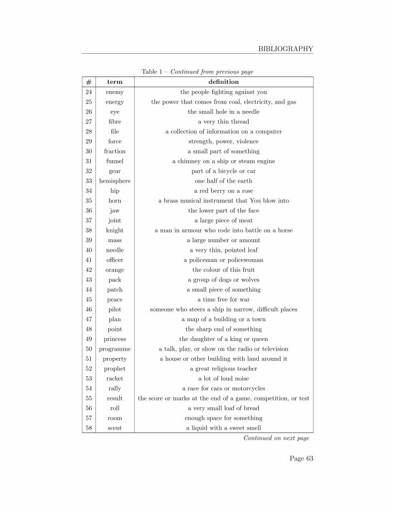
BIBLIOGRAPHY
Table 1 – Continued from previous page
# term definition
24 enemy the people fighting against you
25 energy the power that comes from coal, electricity, and gas
26 eye the small hole in a needle
27 fibre a very thin thread
28 file a collection of information on a computer
29 force strength, power, violence
30 fraction a small part of something
31 funnel a chimney on a ship or steam engine
32 gear part of a bicycle or car
33 hemisphere one half of the earth
34 hip a red berry on a rose
35 horn a brass musical instrument that You blow into
36 jaw the lower part of the face
37 joint a large piece of meat
38 knight a man in armour who rode into battle on a horse
39 mass a large number or amount
40 needle a very thin, pointed leaf
41 o�cer a policeman or policewoman
42 orange the colour of this fruit
43 pack a group of dogs or wolves
44 patch a small piece of something
45 peace a time free for war
46 pilot someone who steers a ship in narrow, di�cult places
47 plan a map of a building or a town
48 point the sharp end of something
49 princess the daughter of a king or queen
50 programme a talk, play, or show on the radio or television
51 property a house or other building with land around it
52 prophet a great religious teacher
53 racket a lot of loud noise
54 rally a race for cars or motorcycles
55 result the score or marks at the end of a game, competition, or test
56 roll a very small loaf of bread
57 room enough space for something
58 scent a liquid with a sweet smell
Continued on next page
Page 63
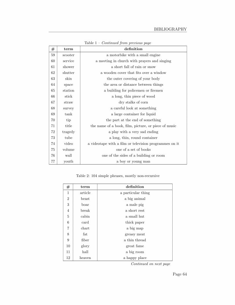
BIBLIOGRAPHY
Table 1 – Continued from previous page
# term definition
59 scooter a motorbike with a small engine
60 service a meeting in church with prayers and singing
61 shower a short fall of rain or snow
62 shutter a wooden cover that fits over a window
63 skin the outer covering of your body
64 space the area or distance between things
65 station a building for policemen or firemen
66 stick a long, thin piece of wood
67 straw dry stalks of corn
68 survey a careful look at something
69 tank a large container for liquid
70 tip the part at the end of something
71 title the name of a book, film, picture, or piece of music
72 tragedy a play with a very sad ending
73 tube a long, thin, round container
74 video a videotape with a film or television programmes on it
75 volume one of a set of books
76 wall one of the sides of a building or room
77 youth a boy or young man
Table 2: 104 simple phrases, mostly non-recursive
# term definition
1 article a particular thing
2 beast a big animal
3 boar a male pig
4 break a short rest
5 cabin a small hut
6 card thick paper
7 chart a big map
8 fat greasy meat
9 fiber a thin thread
10 glory great fame
11 hall a big room
12 heaven a happy place
Continued on next page
Page 64
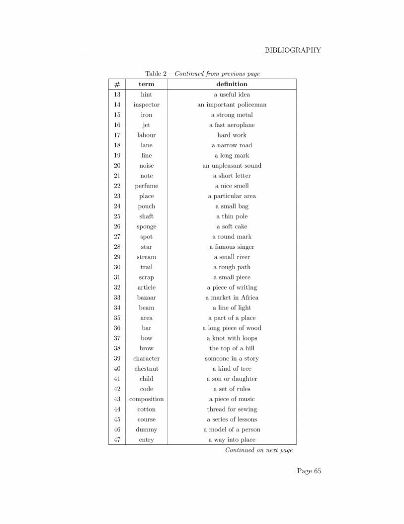
BIBLIOGRAPHY
Table 2 – Continued from previous page
# term definition
13 hint a useful idea
14 inspector an important policeman
15 iron a strong metal
16 jet a fast aeroplane
17 labour hard work
18 lane a narrow road
19 line a long mark
20 noise an unpleasant sound
21 note a short letter
22 perfume a nice smell
23 place a particular area
24 pouch a small bag
25 shaft a thin pole
26 sponge a soft cake
27 spot a round mark
28 star a famous singer
29 stream a small river
30 trail a rough path
31 scrap a small piece
32 article a piece of writing
33 bazaar a market in Africa
34 beam a line of light
35 area a part of a place
36 bar a long piece of wood
37 bow a knot with loops
38 brow the top of a hill
39 character someone in a story
40 chestnut a kind of tree
41 child a son or daughter
42 code a set of rules
43 composition a piece of music
44 cotton thread for sewing
45 course a series of lessons
46 dummy a model of a person
47 entry a way into place
Continued on next page
Page 65
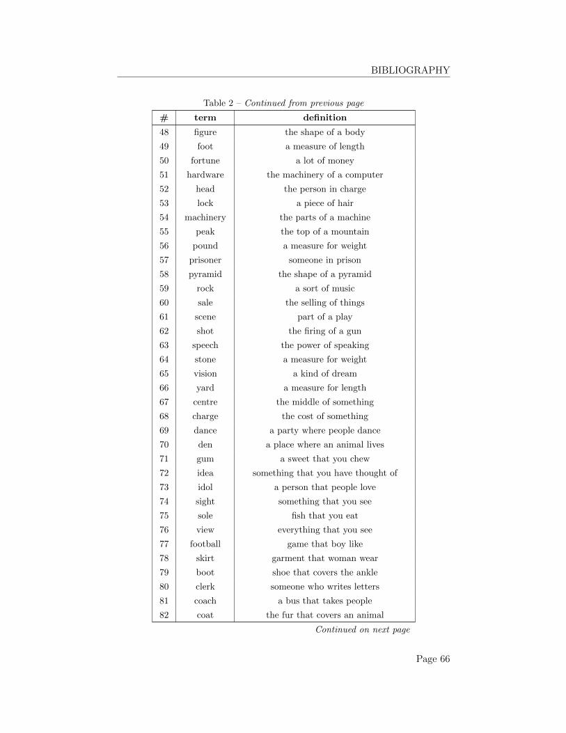
BIBLIOGRAPHY
Table 2 – Continued from previous page
# term definition
48 figure the shape of a body
49 foot a measure of length
50 fortune a lot of money
51 hardware the machinery of a computer
52 head the person in charge
53 lock a piece of hair
54 machinery the parts of a machine
55 peak the top of a mountain
56 pound a measure for weight
57 prisoner someone in prison
58 pyramid the shape of a pyramid
59 rock a sort of music
60 sale the selling of things
61 scene part of a play
62 shot the firing of a gun
63 speech the power of speaking
64 stone a measure for weight
65 vision a kind of dream
66 yard a measure for length
67 centre the middle of something
68 charge the cost of something
69 dance a party where people dance
70 den a place where an animal lives
71 gum a sweet that you chew
72 idea something that you have thought of
73 idol a person that people love
74 sight something that you see
75 sole fish that you eat
76 view everything that you see
77 football game that boy like
78 skirt garment that woman wear
79 boot shoe that covers the ankle
80 clerk someone who writes letters
81 coach a bus that takes people
82 coat the fur that covers an animal
Continued on next page
Page 66
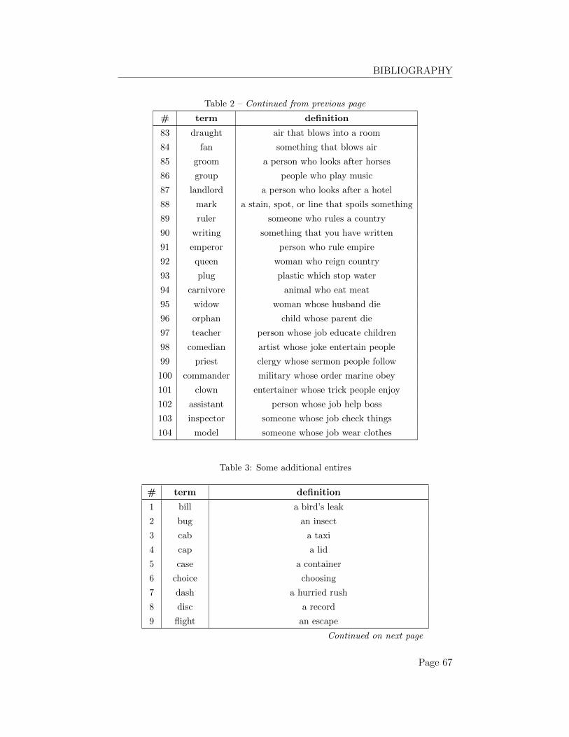
BIBLIOGRAPHY
Table 2 – Continued from previous page
# term definition
83 draught air that blows into a room
84 fan something that blows air
85 groom a person who looks after horses
86 group people who play music
87 landlord a person who looks after a hotel
88 mark a stain, spot, or line that spoils something
89 ruler someone who rules a country
90 writing something that you have written
91 emperor person who rule empire
92 queen woman who reign country
93 plug plastic which stop water
94 carnivore animal who eat meat
95 widow woman whose husband die
96 orphan child whose parent die
97 teacher person whose job educate children
98 comedian artist whose joke entertain people
99 priest clergy whose sermon people follow
100 commander military whose order marine obey
101 clown entertainer whose trick people enjoy
102 assistant person whose job help boss
103 inspector someone whose job check things
104 model someone whose job wear clothes
Table 3: Some additional entires
# term definition
1 bill a bird’s leak
2 bug an insect
3 cab a taxi
4 cap a lid
5 case a container
6 choice choosing
7 dash a hurried rush
8 disc a record
9 flight an escape
Continued on next page
Page 67
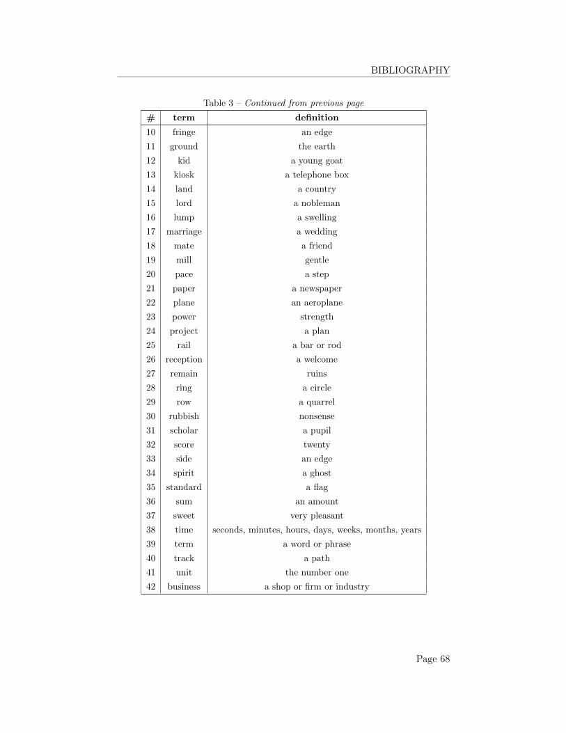
BIBLIOGRAPHY
Table 3 – Continued from previous page
# term definition
10 fringe an edge
11 ground the earth
12 kid a young goat
13 kiosk a telephone box
14 land a country
15 lord a nobleman
16 lump a swelling
17 marriage a wedding
18 mate a friend
19 mill gentle
20 pace a step
21 paper a newspaper
22 plane an aeroplane
23 power strength
24 project a plan
25 rail a bar or rod
26 reception a welcome
27 remain ruins
28 ring a circle
29 row a quarrel
30 rubbish nonsense
31 scholar a pupil
32 score twenty
33 side an edge
34 spirit a ghost
35 standard a flag
36 sum an amount
37 sweet very pleasant
38 time seconds, minutes, hours, days, weeks, months, years
39 term a word or phrase
40 track a path
41 unit the number one
42 business a shop or firm or industry
Page 68
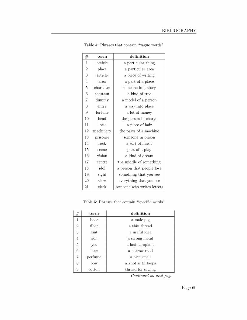
BIBLIOGRAPHY
Table 4: Phrases that contain “vague words”
# term definition
1 article a particular thing
2 place a particular area
3 article a piece of writing
4 area a part of a place
5 character someone in a story
6 chestnut a kind of tree
7 dummy a model of a person
8 entry a way into place
9 fortune a lot of money
10 head the person in charge
11 lock a piece of hair
12 machinery the parts of a machine
13 prisoner someone in prison
14 rock a sort of music
15 scene part of a play
16 vision a kind of dream
17 centre the middle of something
18 idol a person that people love
19 sight something that you see
20 view everything that you see
21 clerk someone who writes letters
Table 5: Phrases that contain “specific words”
# term definition
1 boar a male pig
2 fiber a thin thread
3 hint a useful idea
4 iron a strong metal
5 yet a fast aeroplane
6 lane a narrow road
7 perfume a nice smell
8 bow a knot with loops
9 cotton thread for sewing
Continued on next page
Page 69
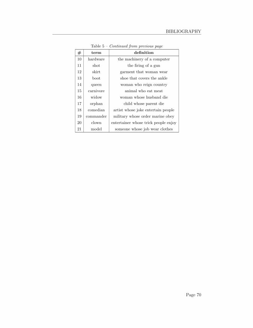
BIBLIOGRAPHY
Table 5 – Continued from previous page
# term definition
10 hardware the machinery of a computer
11 shot the firing of a gun
12 skirt garment that woman wear
13 boot shoe that covers the ankle
14 queen woman who reign country
15 carnivore animal who eat meat
16 widow woman whose husband die
17 orphan child whose parent die
18 comedian artist whose joke entertain people
19 commander military whose order marine obey
20 clown entertainer whose trick people enjoy
21 model someone whose job wear clothes
Page 70