a gentle introduction to haskell 98 · haskell programming experience, and cannot be avoided. 2...

A Gentle Introduction to Haskell 98

Paul HudakYale University

Department of Computer Science

John PetersonYale University

Department of Computer Science

Joseph H. FaselUniversity of California

Los Alamos National Laboratory

October, 1999

Copyright c© 1999 Paul Hudak, John Peterson and Joseph Fasel

Permission is hereby granted, free of charge, to any person obtaining a copy of “A GentleIntroduction to Haskell” (the Text), to deal in the Text without restriction, including withoutlimitation the rights to use, copy, modify, merge, publish, distribute, sublicense, and/or sellcopies of the Text, and to permit persons to whom the Text is furnished to do so, subject to thefollowing condition: The above copyright notice and this permission notice shall be included inall copies or substantial portions of the Text.

1 Introduction

Our purpose in writing this tutorial is not to teach programming, nor even to teach functionalprogramming. Rather, it is intended to serve as a supplement to the Haskell Report [4], whichis otherwise a rather dense technical exposition. Our goal is to provide a gentle introduction toHaskell for someone who has experience with at least one other language, preferably a functionallanguage (even if only an “almost-functional” language such as ML or Scheme). If the readerwishes to learn more about the functional programming style, we highly recommend Bird’s textIntroduction to Functional Programming [1] or Davie’s An Introduction to Functional Program-ming Systems Using Haskell [2]. For a useful survey of functional programming languages andtechniques, including some of the language design principles used in Haskell, see [3].

The Haskell language has evolved significantly since its birth in 1987. This tutorial deals withHaskell 98. Older versions of the language are now obsolete; Haskell users are encouraged to useHaskell 98. There are also many extensions to Haskell 98 that have been widely implemented.These are not yet a formal part of the Haskell language and are not covered in this tutorial.

Our general strategy for introducing language features is this: motivate the idea, define someterms, give some examples, and then point to the Report for details. We suggest, however, thatthe reader completely ignore the details until the Gentle Introduction has been completely read.On the other hand, Haskell’s Standard Prelude (in Appendix A of the Report and the standardlibraries (found in the Library Report [5]) contain lots of useful examples of Haskell code; weencourage a thorough reading once this tutorial is completed. This will not only give the readera feel for what real Haskell code looks like, but will also familiarize her with Haskell’s standardset of predefined functions and types.

1

2 VALUES, TYPES, AND OTHER GOODIES 2

Finally, the Haskell web site, http://haskell.org, has a wealth of information about theHaskell language and its implementations.

[We have also taken the course of not laying out a plethora of lexical syntax rules at theoutset. Rather, we introduce them incrementally as our examples demand, and enclose themin brackets, as with this paragraph. This is in stark contrast to the organization of the Report,although the Report remains the authoritative source for details (references such as “§2.1” referto sections in the Report).]

Haskell is a typeful programming language:1 types are pervasive, and the newcomer is bestoff becoming well aware of the full power and complexity of Haskell’s type system from theoutset. For those whose only experience is with relatively “untypeful” languages such as Perl,Tcl, or Scheme, this may be a difficult adjustment; for those familiar with Java, C, Modula, oreven ML, the adjustment should be easier but still not insignificant, since Haskell’s type systemis different and somewhat richer than most. In any case, “typeful programming” is part of theHaskell programming experience, and cannot be avoided.

2 Values, Types, and Other Goodies

Because Haskell is a purely functional language, all computations are done via the evaluation ofexpressions (syntactic terms) to yield values (abstract entities that we regard as answers). Everyvalue has an associated type. (Intuitively, we can think of types as sets of values.) Examplesof expressions include atomic values such as the integer 5, the character ’a’, and the function\x -> x+1, as well as structured values such as the list [1,2,3] and the pair (’b’,4).

Just as expressions denote values, type expressions are syntactic terms that denote typevalues (or just types). Examples of type expressions include the atomic types Integer (infinite-precision integers), Char (characters), Integer->Integer (functions mapping Integer to Integer),as well as the structured types [Integer] (homogeneous lists of integers) and (Char,Integer)(character, integer pairs).

All Haskell values are “first-class”—they may be passed as arguments to functions, returnedas results, placed in data structures, etc. Haskell types, on the other hand, are not first-class.Types in a sense describe values, and the association of a value with its type is called a typing.Using the examples of values and types above, we write typings as follows:

5 :: Integer’a’ :: Charinc :: Integer -> Integer

[1,2,3] :: [Integer](’b’,4) :: (Char,Integer)

The “::” can be read “has type.”

Functions in Haskell are normally defined by a series of equations. For example, the functioninc can be defined by the single equation:

inc n = n+1

An equation is an example of a declaration. Another kind of declaration is a type signaturedeclaration (§4.4.1), with which we can declare an explicit typing for inc:

inc :: Integer -> Integer

We will have much more to say about function definitions in Section 3.1Coined by Luca Cardelli.


For pedagogical purposes, when we wish to indicate that an expression e1 evaluates, or“reduces,” to another expression or value e2, we will write:

e1 ⇒ e2

For example, note that:inc (inc 3) ⇒ 5

Haskell’s static type system defines the formal relationship between types and values (§4.1.3).The static type system ensures that Haskell programs are type safe; that is, that the programmerhas not mismatched types in some way. For example, we cannot generally add together twocharacters, so the expression ’a’+’b’ is ill-typed. The main advantage of statically typedlanguages is well-known: All type errors are detected at compile-time. Not all errors are caughtby the type system; an expression such as 1/0 is typable but its evaluation will result in an errorat execution time. Still, the type system finds many program errors at compile time, aids theuser in reasoning about programs, and also permits a compiler to generate more efficient code(for example, no run-time type tags or tests are required).

The type system also ensures that user-supplied type signatures are correct. In fact, Haskell’stype system is powerful enough to allow us to avoid writing any type signatures at all;2 we saythat the type system infers the correct types for us. Nevertheless, judicious placement of typesignatures such as that we gave for inc is a good idea, since type signatures are a very effectiveform of documentation and help bring programming errors to light.

[The reader will note that we have capitalized identifiers that denote specific types, suchas Integer and Char, but not identifiers that denote values, such as inc. This is not just aconvention: it is enforced by Haskell’s lexical syntax. In fact, the case of the other charactersmatters, too: foo, fOo, and fOO are all distinct identifiers.]

2.1 Polymorphic Types

Haskell also incorporates polymorphic types—types that are universally quantified in some wayover all types. Polymorphic type expressions essentially describe families of types. For example,(∀a)[a] is the family of types consisting of, for every type a, the type of lists of a. Lists ofintegers (e.g. [1,2,3]), lists of characters ([’a’,’b’,’c’]), even lists of lists of integers, etc.,are all members of this family. (Note, however, that [2,’b’] is not a valid example, since thereis no single type that contains both 2 and ’b’.)

[Identifiers such as a above are called type variables, and are uncapitalized to distinguishthem from specific types such as Int. Furthermore, since Haskell has only universally quantifiedtypes, there is no need to explicitly write out the symbol for universal quantification, and thuswe simply write [a] in the example above. In other words, all type variables are implicitlyuniversally quantified.]

Lists are a commonly used data structure in functional languages, and are a good vehicle forexplaining the principles of polymorphism. The list [1,2,3] in Haskell is actually shorthandfor the list 1:(2:(3:[])), where [] is the empty list and : is the infix operator that adds itsfirst argument to the front of its second argument (a list).3 Since : is right associative, we canalso write this list as 1:2:3:[].

As an example of a user-defined function that operates on lists, consider the problem ofcounting the number of elements in a list:

2With a few exceptions to be described later.3: and [] are like Lisp’s cons and nil, respectively.


length :: [a] -> Integerlength [] = 0length (x:xs) = 1 + length xs

This definition is almost self-explanatory. We can read the equations as saying: “The length ofthe empty list is 0, and the length of a list whose first element is x and remainder is xs is 1 plusthe length of xs.” (Note the naming convention used here; xs is the plural of x, and should beread that way.)

Although intuitive, this example highlights an important aspect of Haskell that is yet to beexplained: pattern matching. The left-hand sides of the equations contain patterns such as []and x:xs. In a function application these patterns are matched against actual parameters in afairly intuitive way ([] only matches the empty list, and x:xs will successfully match any listwith at least one element, binding x to the first element and xs to the rest of the list). If thematch succeeds, the right-hand side is evaluated and returned as the result of the application.If it fails, the next equation is tried, and if all equations fail, an error results.

Defining functions by pattern matching is quite common in Haskell, and the user shouldbecome familiar with the various kinds of patterns that are allowed; we will return to this issuein Section 4.

The length function is also an example of a polymorphic function. It can be applied to alist containing elements of any type, for example [Integer], [Char], or [[Integer]].

length [1,2,3] ⇒ 3length [’a’,’b’,’c’] ⇒ 3length [[1],[2],[3]] ⇒ 3

Here are two other useful polymorphic functions on lists that will be used later. Functionhead returns the first element of a list, function tail returns all but the first.

head :: [a] -> ahead (x:xs) = x

tail :: [a] -> [a]tail (x:xs) = xs

Unlike length, these functions are not defined for all possible values of their argument. Aruntime error occurs when these functions are applied to an empty list.

With polymorphic types, we find that some types are in a sense strictly more general thanothers in the sense that the set of values they define is larger. For example, the type [a] is moregeneral than [Char]. In other words, the latter type can be derived from the former by a suitablesubstitution for a. With regard to this generalization ordering, Haskell’s type system possessestwo important properties: First, every well-typed expression is guaranteed to have a uniqueprincipal type (explained below), and second, the principal type can be inferred automatically(§4.1.3). In comparison to a monomorphically typed language such as C, the reader will findthat polymorphism improves expressiveness, and type inference lessens the burden of types onthe programmer.

An expression’s or function’s principal type is the least general type that, intuitively, “con-tains all instances of the expression”. For example, the principal type of head is [a]->a; [b]->a,a->a, or even a are correct types, but too general, whereas something like [Integer]->Integeris too specific. The existence of unique principal types is the hallmark feature of the Hindley-Milner type system, which forms the basis of the type systems of Haskell, ML, Miranda,4 andseveral other (mostly functional) languages.

4“Miranda” is a trademark of Research Software, Ltd.


2.2 User-Defined Types

We can define our own types in Haskell using a data declaration, which we introduce via a seriesof examples (§4.2.1).

An important predefined type in Haskell is that of truth values:

data Bool = False | True

The type being defined here is Bool, and it has exactly two values: True and False. TypeBool is an example of a (nullary) type constructor, and True and False are (also nullary) dataconstructors (or just constructors, for short).

Similarly, we might wish to define a color type:

data Color = Red | Green | Blue | Indigo | Violet

Both Bool and Color are examples of enumerated types, since they consist of a finite numberof nullary data constructors.

Here is an example of a type with just one data constructor:

data Point a = Pt a a

Because of the single constructor, a type like Point is often called a tuple type, since it isessentially just a cartesian product (in this case binary) of other types.5 In contrast, multi-constructor types, such as Bool and Color, are called (disjoint) union or sum types.

More importantly, however, Point is an example of a polymorphic type: for any type t,it defines the type of cartesian points that use t as the coordinate type. The Point type cannow be seen clearly as a unary type constructor, since from the type t it constructs a new typePoint t. (In the same sense, using the list example given earlier, [] is also a type constructor.Given any type t we can “apply” [] to yield a new type [t]. The Haskell syntax allows [] t tobe written as [t]. Similarly, -> is a type constructor: given two types t and u, t->u is the typeof functions mapping elements of type t to elements of type u.)

Note that the type of the binary data constructor Pt is a -> a -> Point a, and thus thefollowing typings are valid:

Pt 2.0 3.0 :: Point FloatPt ’a’ ’b’ :: Point CharPt True False :: Point Bool

On the other hand, an expression such as Pt ’a’ 1 is ill-typed because ’a’ and 1 are of differenttypes.

It is important to distinguish between applying a data constructor to yield a value, andapplying a type constructor to yield a type; the former happens at run-time and is how wecompute things in Haskell, whereas the latter happens at compile-time and is part of the typesystem’s process of ensuring type safety.

[Type constructors such as Point and data constructors such as Pt are in separate names-paces. This allows the same name to be used for both a type constructor and data constructor,as in the following:

data Point a = Point a a

While this may seem a little confusing at first, it serves to make the link between a type and itsdata constructor more obvious.]

5Tuples are somewhat like records in other languages.


2.2.1 Recursive Types

Types can also be recursive, as in the type of binary trees:

data Tree a = Leaf a | Branch (Tree a) (Tree a)

Here we have defined a polymorphic binary tree type whose elements are either leaf nodescontaining a value of type a, or internal nodes (“branches”) containing (recursively) two sub-trees.

When reading data declarations such as this, remember again that Tree is a type constructor,whereas Branch and Leaf are data constructors. Aside from establishing a connection betweenthese constructors, the above declaration is essentially defining the following types for Branchand Leaf:

Branch :: Tree a -> Tree a -> Tree aLeaf :: a -> Tree a

With this example we have defined a type sufficiently rich to allow defining some interesting(recursive) functions that use it. For example, suppose we wish to define a function fringethat returns a list of all the elements in the leaves of a tree from left to right. It’s usuallyhelpful to write down the type of new functions first; in this case we see that the type shouldbe Tree a -> [a]. That is, fringe is a polymorphic function that, for any type a, maps treesof a into lists of a. A suitable definition follows:

fringe :: Tree a -> [a]fringe (Leaf x) = [x]fringe (Branch left right) = fringe left ++ fringe right

Here ++ is the infix operator that concatenates two lists (its full definition will be given inSection 9.1). As with the length example given earlier, the fringe function is defined usingpattern matching, except that here we see patterns involving user-defined constructors: Leafand Branch. [Note that the formal parameters are easily identified as the ones beginning withlower-case letters.]

2.3 Type Synonyms

For convenience, Haskell provides a way to define type synonyms; i.e. names for commonly usedtypes. Type synonyms are created using a type declaration (§4.2.2). Here are several examples:

type String = [Char]type Person = (Name,Address)type Name = Stringdata Address = None | Addr String

Type synonyms do not define new types, but simply give new names for existing types. Forexample, the type Person -> Name is precisely equivalent to (String,Address) -> String.The new names are often shorter than the types they are synonymous with, but this is notthe only purpose of type synonyms: they can also improve readability of programs by beingmore mnemonic; indeed, the above examples highlight this. We can even give new names topolymorphic types:

type AssocList a b = [(a,b)]

This is the type of “association lists” which associate values of type a with those of type b.


2.4 Built-in Types Are Not Special

Earlier we introduced several “built-in” types such as lists, tuples, integers, and characters. Wehave also shown how new user-defined types can be defined. Aside from special syntax, are thebuilt-in types in any way more special than the user-defined ones? The answer is no. The specialsyntax is for convenience and for consistency with historical convention, but has no semanticconsequences.

We can emphasize this point by considering what the type declarations would look like forthese built-in types if in fact we were allowed to use the special syntax in defining them. Forexample, the Char type might be written as:

data Char = ’a’ | ’b’ | ’c’ | ... -- This is not valid| ’A’ | ’B’ | ’C’ | ... -- Haskell code!| ’1’ | ’2’ | ’3’ | ......

These constructor names are not syntactically valid; to fix them we would have to write some-thing like:

data Char = Ca | Cb | Cc | ...| CA | CB | CC | ...| C1 | C2 | C3 | ......

Even though these constructors are more concise, they are quite unconventional for representingcharacters.

In any case, writing “pseudo-Haskell” code in this way helps us to see through the specialsyntax. We see now that Char is just an enumerated type consisting of a large number of nullaryconstructors. Thinking of Char in this way makes it clear that we can pattern-match againstcharacters in function definitions, just as we would expect to be able to do so for any of a type’sconstructors.

[This example also demonstrates the use of comments in Haskell; the characters -- and allsubsequent characters to the end of the line are ignored. Haskell also permits nested commentswhich have the form {-. . .-} and can appear anywhere (§2.2).]

Similarly, we could define Int (fixed precision integers) and Integer by:

data Int = -65532 | ... | -1 | 0 | 1 | ... | 65532 -- more pseudo-codedata Integer = ... -2 | -1 | 0 | 1 | 2 ...

where -65532 and 65532, say, are the maximum and minimum fixed precision integers for agiven implementation. Int is a much larger enumeration than Char, but it’s still finite! Incontrast, the pseudo-code for Integer is intended to convey an infinite enumeration.

Tuples are also easy to define playing this game:

data (a,b) = (a,b) -- more pseudo-codedata (a,b,c) = (a,b,c)data (a,b,c,d) = (a,b,c,d). .. .. .

Each declaration above defines a tuple type of a particular length, with (...) playing a role inboth the expression syntax (as data constructor) and type-expression syntax (as type construc-tor). The vertical dots after the last declaration are intended to convey an infinite number ofsuch declarations, reflecting the fact that tuples of all lengths are allowed in Haskell.


Lists are also easily handled, and more interestingly, they are recursive:

data [a] = [] | a : [a] -- more pseudo-code

We can now see clearly what we described about lists earlier: [] is the empty list, and : isthe infix list constructor; thus [1,2,3] must be equivalent to the list 1:2:3:[]. (: is rightassociative.) The type of [] is [a], and the type of : is a->[a]->[a].

[The way “:” is defined here is actually legal syntax—infix constructors are permitted indata declarations, and are distinguished from infix operators (for pattern-matching purposes)by the fact that they must begin with a “:” (a property trivially satisfied by “:”).]

At this point the reader should note carefully the differences between tuples and lists, whichthe above definitions make abundantly clear. In particular, note the recursive nature of the listtype whose elements are homogeneous and of arbitrary length, and the non-recursive nature of a(particular) tuple type whose elements are heterogeneous and of fixed length. The typing rulesfor tuples and lists should now also be clear:

For (e1,e2, . . . ,en), n ≥ 2, if ti is the type of ei, then the type of the tuple is (t1,t2, . . . ,tn).

For [e1,e2, . . . ,en], n ≥ 0, each ei must have the same type t, and the type of the list is[t].

2.4.1 List Comprehensions and Arithmetic Sequences

As with Lisp dialects, lists are pervasive in Haskell, and as with other functional languages, thereis yet more syntactic sugar to aid in their creation. Aside from the constructors for lists justdiscussed, Haskell provides an expression known as a list comprehension that is best explainedby example:

[ f x | x <- xs ]

This expression can intuitively be read as “the list of all f x such that x is drawn from xs.”The similarity to set notation is not a coincidence. The phrase x <- xs is called a generator, ofwhich more than one is allowed, as in:

[ (x,y) | x <- xs, y <- ys ]

This list comprehension forms the cartesian product of the two lists xs and ys. The elementsare selected as if the generators were “nested” from left to right (with the rightmost generatorvarying fastest); thus, if xs is [1,2] and ys is [3,4], the result is [(1,3),(1,4),(2,3),(2,4)].

Besides generators, boolean expressions called guards are permitted. Guards place con-straints on the elements generated. For example, here is a concise definition of everybody’sfavorite sorting algorithm:

quicksort [] = []quicksort (x:xs) = quicksort [y | y <- xs, y<x ]

++ [x]++ quicksort [y | y <- xs, y>=x]

To further support the use of lists, Haskell has special syntax for arithmetic sequences, whichare best explained by a series of examples:

[1..10] ⇒ [1,2,3,4,5,6,7,8,9,10][1,3..10] ⇒ [1,3,5,7,9][1,3..] ⇒ [1,3,5,7,9, ... (infinite sequence)

More will be said about arithmetic sequences in Section 8.2, and “infinite lists” in Section 3.4.

3 FUNCTIONS 9

2.4.2 Strings

As another example of syntactic sugar for built-in types, we note that the literal string "hello"is actually shorthand for the list of characters [’h’,’e’,’l’,’l’,’o’]. Indeed, the type of"hello" is String, where String is a predefined type synonym (that we gave as an earlierexample):

type String = [Char]

This means we can use predefined polymorphic list functions to operate on strings. For example:

"hello" ++ " world" ⇒ "hello world"

3 Functions

Since Haskell is a functional language, one would expect functions to play a major role, andindeed they do. In this section, we look at several aspects of functions in Haskell.

First, consider this definition of a function which adds its two arguments:

add :: Integer -> Integer -> Integeradd x y = x + y

This is an example of a curried function.6 An application of add has the form add e1 e2,and is equivalent to (add e1) e2, since function application associates to the left. In otherwords, applying add to one argument yields a new function which is then applied to the secondargument. This is consistent with the type of add, Integer->Integer->Integer, which isequivalent to Integer->(Integer->Integer); i.e. -> associates to the right. Indeed, using add,we can define inc in a different way from earlier:

inc = add 1

This is an example of the partial application of a curried function, and is one way that a functioncan be returned as a value. Let’s consider a case in which it’s useful to pass a function as anargument. The well-known map function is a perfect example:

map :: (a->b) -> [a] -> [b]map f [] = []map f (x:xs) = f x : map f xs

[Function application has higher precedence than any infix operator, and thus the right-handside of the second equation parses as (f x) : (map f xs).] The map function is polymorphicand its type indicates clearly that its first argument is a function; note also that the two a’smust be instantiated with the same type (likewise for the b’s). As an example of the use of map,we can increment the elements in a list:

map (add 1) [1,2,3] ⇒ [2,3,4]

These examples demonstrate the first-class nature of functions, which when used in this wayare usually called higher-order functions.

6The name curry derives from the person who popularized the idea: Haskell Curry. To get the effect of anuncurried function, we could use a tuple, as in:

add (x,y) = x + y

But then we see that this version of add is really just a function of one argument!

3 FUNCTIONS 10

3.1 Lambda Abstractions

Instead of using equations to define functions, we can also define them “anonymously” via alambda abstraction. For example, a function equivalent to inc could be written as \x -> x+1.Similarly, the function add is equivalent to \x -> \y -> x+y. Nested lambda abstractions suchas this may be written using the equivalent shorthand notation \x y -> x+y. In fact, theequations:

inc x = x+1add x y = x+y

are really shorthand for:

inc = \x -> x+1add = \x y -> x+y

We will have more to say about such equivalences later.

In general, given that x has type t1 and exp has type t2, then \x->exp has type t1->t2.

3.2 Infix Operators

Infix operators are really just functions, and can also be defined using equations. For example,here is a definition of a list concatenation operator:

(++) :: [a] -> [a] -> [a][] ++ ys = ys(x:xs) ++ ys = x : (xs++ys)

[Lexically, infix operators consist entirely of “symbols,” as opposed to normal identifiers whichare alphanumeric (§2.4). Haskell has no prefix operators, with the exception of minus (-), whichis both infix and prefix.]

As another example, an important infix operator on functions is that for function composi-tion:

(.) :: (b->c) -> (a->b) -> (a->c)f . g = \ x -> f (g x)

3.2.1 Sections

Since infix operators are really just functions, it makes sense to be able to partially apply themas well. In Haskell the partial application of an infix operator is called a section. For example:

(x+) ≡ \y -> x+y(+y) ≡ \x -> x+y(+) ≡ \x y -> x+y

[The parentheses are mandatory.]

The last form of section given above essentially coerces an infix operator into an equivalentfunctional value, and is handy when passing an infix operator as an argument to a function,as in map (+) [1,2,3] (the reader should verify that this returns a list of functions!). It isalso necessary when giving a function type signature, as in the examples of (++) and (.) givenearlier.

We can now see that add defined earlier is just (+), and inc is just (+1)! Indeed, thesedefinitions would do just fine:

3 FUNCTIONS 11

inc = (+ 1)add = (+)

We can coerce an infix operator into a functional value, but can we go the other way?Yes—we simply enclose an identifier bound to a functional value in backquotes. For example,x ‘add‘ y is the same as add x y.7 Some functions read better this way. An example is thepredefined list membership predicate elem; the expression x ‘elem‘ xs can be read intuitivelyas “x is an element of xs.”

[There are some special rules regarding sections involving the prefix/infix operator -; see(§3.5,§3.4).]

At this point, the reader may be confused at having so many ways to define a function! Thedecision to provide these mechanisms partly reflects historical conventions, and partly reflectsthe desire for consistency (for example, in the treatment of infix vs. regular functions).

3.2.2 Fixity Declarations

A fixity declaration can be given for any infix operator or constructor (including those madefrom ordinary identifiers, such as ‘elem‘). This declaration specifies a precedence level from 0to 9 (with 9 being the strongest; normal application is assumed to have a precedence level of10), and left-, right-, or non-associativity. For example, the fixity declarations for ++ and . are:

infixr 5 ++infixr 9 .

Both of these specify right-associativity, the first with a precedence level of 5, the other 9. Leftassociativity is specified via infixl, and non-associativity by infix. Also, the fixity of morethan one operator may be specified with the same fixity declaration. If no fixity declaration isgiven for a particular operator, it defaults to infixl 9. (See §5.9 for a detailed definition of theassociativity rules.)

3.3 Functions are Non-strict

Suppose bot is defined by:

bot = bot

In other words, bot is a non-terminating expression. Abstractly, we denote the value of a non-terminating expression as ⊥ (read “bottom”). Expressions that result in some kind of a run-timeerror, such as 1/0, also have this value. Such an error is not recoverable: programs will notcontinue past these errors. Errors encountered by the I/O system, such as an end-of-file error,are recoverable and are handled in a different manner. (Such an I/O error is really not an errorat all but rather an exception. Much more will be said about exceptions in Section 7.)

A function f is said to be strict if, when applied to a nonterminating expression, it also failsto terminate. In other words, f is strict iff the value of f bot is ⊥. For most programminglanguages, all functions are strict. But this is not so in Haskell. As a simple example, considerconst1, the constant 1 function, defined by:

const1 x = 1

The value of const1 bot in Haskell is 1. Operationally speaking, since const1 does not “need”7Note carefully that add is enclosed in backquotes, not apostrophes as used in the syntax of characters; i.e. ’f’

is a character, whereas ‘f‘ is an infix operator. Fortunately, most ASCII terminals distinguish these much betterthan the font used in this manuscript.

3 FUNCTIONS 12

the value of its argument, it never attempts to evaluate it, and thus never gets caught in a non-terminating computation. For this reason, non-strict functions are also called “lazy functions”,and are said to evaluate their arguments “lazily”, or “by need”.

Since error and nonterminating values are semantically the same in Haskell, the above argu-ment also holds for errors. For example, const1 (1/0) also evaluates properly to 1.

Non-strict functions are extremely useful in a variety of contexts. The main advantage isthat they free the programmer from many concerns about evaluation order. Computationallyexpensive values may be passed as arguments to functions without fear of them being computedif they are not needed. An important example of this is a possibly infinite data structure.

Another way of explaining non-strict functions is that Haskell computes using definitionsrather than the assignments found in traditional languages. Read a declaration such as

v = 1/0

as ‘define v as 1/0’ instead of ‘compute 1/0 and store the result in v’. Only if the value(definition) of v is needed will the division by zero error occur. By itself, this declaration doesnot imply any computation. Programming using assignments requires careful attention to theordering of the assignments: the meaning of the program depends on the order in which theassignments are executed. Definitions, in contrast, are much simpler: they can be presented inany order without affecting the meaning of the program.

3.4 “Infinite” Data Structures

One advantage of the non-strict nature of Haskell is that data constructors are non-strict, too.This should not be surprising, since constructors are really just a special kind of function (thedistinguishing feature being that they can be used in pattern matching). For example, theconstructor for lists, (:), is non-strict.

Non-strict constructors permit the definition of (conceptually) infinite data structures. Hereis an infinite list of ones:

ones = 1 : ones

Perhaps more interesting is the function numsFrom:

numsFrom n = n : numsFrom (n+1)

Thus numsFrom n is the infinite list of successive integers beginning with n. From it we canconstruct an infinite list of squares:

squares = map (^2) (numsfrom 0)

(Note the use of a section; ^ is the infix exponentiation operator.)

Of course, eventually we expect to extract some finite portion of the list for actual compu-tation, and there are lots of predefined functions in Haskell that do this sort of thing: take,takeWhile, filter, and others. The definition of Haskell includes a large set of built-in func-tions and types—this is called the “Standard Prelude”. The complete Standard Prelude isincluded in Appendix A of the Haskell report; see the portion named PreludeList for manyuseful functions involving lists. For example, take removes the first n elements from a list:

take 5 squares ⇒ [0,1,4,9,16]

The definition of ones above is an example of a circular list. In most circumstances lazinesshas an important impact on efficiency, since an implementation can be expected to implementthe list as a true circular structure, thus saving space.

4 CASE EXPRESSIONS AND PATTERN MATCHING 13

Figure 1: Circular Fibonacci Sequence

For another example of the use of circularity, the Fibonacci sequence can be computedefficiently as the following infinite sequence:

fib = 1 : 1 : [ a+b | (a,b) <- zip fib (tail fib) ]

where zip is a Standard Prelude function that returns the pairwise interleaving of its two listarguments:

zip (x:xs) (y:ys) = (x,y) : zip xs yszip xs ys = []

Note how fib, an infinite list, is defined in terms of itself, as if it were “chasing its tail.” Indeed,we can draw a picture of this computation as shown in Figure 1.

For another application of infinite lists, see Section 4.4.

3.5 The Error Function

Haskell has a built-in function called error whose type is String->a. This is a somewhat oddfunction: From its type it looks as if it is returning a value of a polymorphic type about whichit knows nothing, since it never receives a value of that type as an argument!

In fact, there is one value “shared” by all types: ⊥. Indeed, semantically that is exactlywhat value is always returned by error (recall that all errors have value ⊥). However, we canexpect that a reasonable implementation will print the string argument to error for diagnosticpurposes. Thus this function is useful when we wish to terminate a program when somethinghas “gone wrong.” For example, the actual definition of head taken from the Standard Preludeis:

head (x:xs) = xhead [] = error "head{PreludeList}: head []"

4 Case Expressions and Pattern Matching

Earlier we gave several examples of pattern matching in defining functions—for example lengthand fringe. In this section we will look at the pattern-matching process in greater detail(§3.17).8

8Pattern matching in Haskell is different from that found in logic programming languages such as Prolog; inparticular, it can be viewed as “one-way” matching, whereas Prolog allows “two-way” matching (via unification),along with implicit backtracking in its evaluation mechanism.


Patterns are not “first-class;” there is only a fixed set of different kinds of patterns. We havealready seen several examples of data constructor patterns; both length and fringe definedearlier use such patterns, the former on the constructors of a “built-in” type (lists), the latter ona user-defined type (Tree). Indeed, matching is permitted using the constructors of any type,user-defined or not. This includes tuples, strings, numbers, characters, etc. For example, here’sa contrived function that matches against a tuple of “constants:”

contrived :: ([a], Char, (Int, Float), String, Bool) -> Boolcontrived ([], ’b’, (1, 2.0), "hi", True) = False

This example also demonstrates that nesting of patterns is permitted (to arbitrary depth).

Technically speaking, formal parameters9 are also patterns—it’s just that they never fail tomatch a value. As a “side effect” of the successful match, the formal parameter is bound to thevalue it is being matched against. For this reason patterns in any one equation are not allowedto have more than one occurrence of the same formal parameter (a property called linearity§3.17, §3.3, §4.4.2).

Patterns such as formal parameters that never fail to match are said to be irrefutable, incontrast to refutable patterns which may fail to match. The pattern used in the contrivedexample above is refutable. There are three other kinds of irrefutable patterns, two of which wewill introduce now (the other we will delay until Section 4.4).

As-patterns. Sometimes it is convenient to name a pattern for use on the right-hand side ofan equation. For example, a function that duplicates the first element in a list might be writtenas:

f (x:xs) = x:x:xs

(Recall that “:” associates to the right.) Note that x:xs appears both as a pattern on the left-hand side, and an expression on the right-hand side. To improve readability, we might prefer towrite x:xs just once, which we can achieve using an as-pattern as follows:10

f s@(x:xs) = x:s

Technically speaking, as-patterns always result in a successful match, although the sub-pattern(in this case x:xs) could, of course, fail.

Wild-cards. Another common situation is matching against a value we really care nothingabout. For example, the functions head and tail defined in Section 2.1 can be rewritten as:

head (x:_) = xtail (_:xs) = xs

in which we have “advertised” the fact that we don’t care what a certain part of the input is.Each wild-card independently matches anything, but in contrast to a formal parameter, eachbinds nothing; for this reason more than one is allowed in an equation.

4.1 Pattern-Matching Semantics

So far we have discussed how individual patterns are matched, how some are refutable, some areirrefutable, etc. But what drives the overall process? In what order are the matches attempted?What if none succeeds? This section addresses these questions.

9The Report calls these variables.10Another advantage to doing this is that a naive implementation might completely reconstruct x:xs rather

than re-use the value being matched against.


Pattern matching can either fail, succeed or diverge. A successful match binds the formalparameters in the pattern. Divergence occurs when a value needed by the pattern contains anerror (⊥). The matching process itself occurs “top-down, left-to-right.” Failure of a patternanywhere in one equation results in failure of the whole equation, and the next equation is thentried. If all equations fail, the value of the function application is ⊥, and results in a run-timeerror.

For example, if [1,2] is matched against [0,bot], then 1 fails to match 0, so the result isa failed match. (Recall that bot, defined earlier, is a variable bound to ⊥.) But if [1,2] ismatched against [bot,0], then matching 1 against bot causes divergence (i.e. ⊥).

The other twist to this set of rules is that top-level patterns may also have a boolean guard,as in this definition of a function that forms an abstract version of a number’s sign:

sign x | x > 0 = 1| x == 0 = 0| x < 0 = -1

Note that a sequence of guards may be provided for the same pattern; as with patterns, theyare evaluated top-down, and the first that evaluates to True results in a successful match.

4.2 An Example

The pattern-matching rules can have subtle effects on the meaning of functions. For example,consider this definition of take:

take 0 _ = []take _ [] = []take n (x:xs) = x : take (n-1) xs

and this slightly different version (the first 2 equations have been reversed):

take1 _ [] = []take1 0 _ = []take1 n (x:xs) = x : take1 (n-1) xs

Now note the following:take 0 bot ⇒ []take1 0 bot ⇒ ⊥

take bot [] ⇒ ⊥take1 bot [] ⇒ []

We see that take is “more defined” with respect to its second argument, whereas take1 is moredefined with respect to its first. It is difficult to say in this case which definition is better.Just remember that in certain applications, it may make a difference. (The Standard Preludeincludes a definition corresponding to take.)

4.3 Case Expressions

Pattern matching provides a way to “dispatch control” based on structural properties of a value.In many circumstances we don’t wish to define a function every time we need to do this, butso far we have only shown how to do pattern matching in function definitions. Haskell’s caseexpression provides a way to solve this problem. Indeed, the meaning of pattern matching infunction definitions is specified in the Report in terms of case expressions, which are considered


more primitive. In particular, a function definition of the form:

f p11 . . . p1k = e1

. . .f pn1 . . . pnk = en

where each pij is a pattern, is semantically equivalent to:

f x1 x2 . . . xk = case (x1, . . . , xk) of (p11 , . . . , p1k) -> e1

. . .(pn1 , . . . , pnk) -> en

where the xi are new identifiers. (For a more general translation that includes guards, see§4.4.2.) For example, the definition of take given earlier is equivalent to:

take m ys = case (m,ys) of(0,_) -> [](_,[]) -> [](n,x:xs) -> x : take (n-1) xs

A point not made earlier is that, for type correctness, the types of the right-hand sides of acase expression or set of equations comprising a function definition must all be the same; moreprecisely, they must all share a common principal type.

The pattern-matching rules for case expressions are the same as we have given for functiondefinitions, so there is really nothing new to learn here, other than to note the convenience thatcase expressions offer. Indeed, there’s one use of a case expression that is so common that it hasspecial syntax: the conditional expression. In Haskell, conditional expressions have the familiarform:

if e1 then e2 else e3

which is really short-hand for:

case e1 of True -> e2

False -> e3

From this expansion it should be clear that e1 must have type Bool, and e2 and e3 must have thesame (but otherwise arbitrary) type. In other words, if-then-else when viewed as a functionhas type Bool->a->a->a.

4.4 Lazy Patterns

There is one other kind of pattern allowed in Haskell. It is called a lazy pattern, and has the form~pat. Lazy patterns are irrefutable: matching a value v against ~pat always succeeds, regardlessof pat. Operationally speaking, if an identifier in pat is later “used” on the right-hand-side, itwill be bound to that portion of the value that would result if v were to successfully match pat,and ⊥ otherwise.

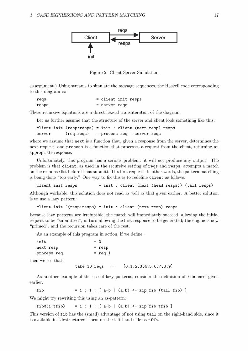
Lazy patterns are useful in contexts where infinite data structures are being defined recur-sively. For example, infinite lists are an excellent vehicle for writing simulation programs, and inthis context the infinite lists are often called streams. Consider the simple case of simulating theinteractions between a server process server and a client process client, where client sends asequence of requests to server, and server replies to each request with some kind of response.This situation is shown pictorially in Figure 2. (Note that client also takes an initial message


Figure 2: Client-Server Simulation

as argument.) Using streams to simulate the message sequences, the Haskell code correspondingto this diagram is:

reqs = client init respsresps = server reqs

These recursive equations are a direct lexical transliteration of the diagram.

Let us further assume that the structure of the server and client look something like this:

client init (resp:resps) = init : client (next resp) respsserver (req:reqs) = process req : server reqs

where we assume that next is a function that, given a response from the server, determines thenext request, and process is a function that processes a request from the client, returning anappropriate response.

Unfortunately, this program has a serious problem: it will not produce any output! Theproblem is that client, as used in the recursive setting of reqs and resps, attempts a matchon the response list before it has submitted its first request! In other words, the pattern matchingis being done “too early.” One way to fix this is to redefine client as follows:

client init resps = init : client (next (head resps)) (tail resps)

Although workable, this solution does not read as well as that given earlier. A better solutionis to use a lazy pattern:

client init ~(resp:resps) = init : client (next resp) resps

Because lazy patterns are irrefutable, the match will immediately succeed, allowing the initialrequest to be “submitted”, in turn allowing the first response to be generated; the engine is now“primed”, and the recursion takes care of the rest.

As an example of this program in action, if we define:

init = 0next resp = respprocess req = req+1

then we see that:take 10 reqs ⇒ [0,1,2,3,4,5,6,7,8,9]

As another example of the use of lazy patterns, consider the definition of Fibonacci givenearlier:

fib = 1 : 1 : [ a+b | (a,b) <- zip fib (tail fib) ]

We might try rewriting this using an as-pattern:

fib@(1:tfib) = 1 : 1 : [ a+b | (a,b) <- zip fib tfib ]

This version of fib has the (small) advantage of not using tail on the right-hand side, since itis available in “destructured” form on the left-hand side as tfib.


[This kind of equation is called a pattern binding because it is a top-level equation in whichthe entire left-hand side is a pattern; i.e. both fib and tfib become bound within the scope ofthe declaration.]

Now, using the same reasoning as earlier, we should be led to believe that this programwill not generate any output. Curiously, however, it does, and the reason is simple: in Haskell,pattern bindings are assumed to have an implicit ~ in front of them, reflecting the most commonbehavior expected of pattern bindings, and avoiding some anomalous situations which are beyondthe scope of this tutorial. Thus we see that lazy patterns play an important role in Haskell, ifonly implicitly.

4.5 Lexical Scoping and Nested Forms

It is often desirable to create a nested scope within an expression, for the purpose of creatinglocal bindings not seen elsewhere—i.e. some kind of “block-structuring” form. In Haskell thereare two ways to achieve this:

Let Expressions. Haskell’s let expressions are useful whenever a nested set of bindings isrequired. As a simple example, consider:

let y = a*bf x = (x+y)/y

in f c + f d

The set of bindings created by a let expression is mutually recursive, and pattern bindings aretreated as lazy patterns (i.e. they carry an implicit ~). The only kind of declarations permittedare type signatures, function bindings, and pattern bindings.

Where Clauses. Sometimes it is convenient to scope bindings over several guarded equations,which requires a where clause:

f x y | y>z = ...| y==z = ...| y<z = ...

where z = x*x

Note that this cannot be done with a let expression, which only scopes over the expressionwhich it encloses. A where clause is only allowed at the top level of a set of equations or caseexpression. The same properties and constraints on bindings in let expressions apply to thosein where clauses.

These two forms of nested scope seem very similar, but remember that a let expression isan expression, whereas a where clause is not—it is part of the syntax of function declarationsand case expressions.

4.6 Layout

The reader may have been wondering how it is that Haskell programs avoid the use of semicolons,or some other kind of terminator, to mark the end of equations, declarations, etc. For example,consider this let expression from the last section:

let y = a*bf x = (x+y)/y

in f c + f d

5 TYPE CLASSES AND OVERLOADING 19

How does the parser know not to parse this as:

let y = a*b fx = (x+y)/y

in f c + f d

?

The answer is that Haskell uses a two-dimensional syntax called layout that essentially relieson declarations being “lined up in columns.” In the above example, note that y and f begin inthe same column. The rules for layout are spelled out in detail in the Report (§2.7, §B.3), butin practice, use of layout is rather intuitive. Just remember two things:

First, the next character following any of the keywords where, let, or of is what determinesthe starting column for the declarations in the where, let, or case expression being written (therule also applies to where used in the class and instance declarations to be introduced in Section5). Thus we can begin the declarations on the same line as the keyword, the next line, etc. (Thedo keyword, to be discussed later, also uses layout).

Second, just be sure that the starting column is further to the right than the starting columnassociated with the immediately surrounding clause (otherwise it would be ambiguous). The“termination” of a declaration happens when something appears at or to the left of the startingcolumn associated with that binding form.11

Layout is actually shorthand for an explicit grouping mechanism, which deserves mentionbecause it can be useful under certain circumstances. The let example above is equivalent to:

let { y = a*b; f x = (x+y)/y}

in f c + f d

Note the explicit curly braces and semicolons. One way in which this explicit notation is usefulis when more than one declaration is desired on a line; for example, this is a valid expression:

let y = a*b; z = a/bf x = (x+y)/z

in f c + f d

For another example of the expansion of layout into explicit delimiters, see §2.7.

The use of layout greatly reduces the syntactic clutter associated with declaration lists, thusenhancing readability. It is easy to learn, and its use is encouraged.

5 Type Classes and Overloading

There is one final feature of Haskell’s type system that sets it apart from other programminglanguages. The kind of polymorphism that we have talked about so far is commonly calledparametric polymorphism. There is another kind called ad hoc polymorphism, better known asoverloading. Here are some examples of ad hoc polymorphism:

• The literals 1, 2, etc. are often used to represent both fixed and arbitrary precision integers.

• Numeric operators such as + are often defined to work on many different kinds of numbers.11Haskell observes the convention that tabs count as 8 blanks; thus care must be taken when using an editor

which may observe some other convention.


• The equality operator (== in Haskell) usually works on numbers and many other (but notall) types.

Note that these overloaded behaviors are different for each type (in fact the behavior is some-times undefined, or error), whereas in parametric polymorphism the type truly does not matter(fringe, for example, really doesn’t care what kind of elements are found in the leaves of atree). In Haskell, type classes provide a structured way to control ad hoc polymorphism, oroverloading.

Let’s start with a simple, but important, example: equality. There are many types for whichwe would like equality defined, but some for which we would not. For example, comparing theequality of functions is generally considered computationally intractable, whereas we often wantto compare two lists for equality.12 To highlight the issue, consider this definition of the functionelem which tests for membership in a list:

x ‘elem‘ [] = Falsex ‘elem‘ (y:ys) = x==y || (x ‘elem‘ ys)

[For the stylistic reason we discussed in Section 3.1, we have chosen to define elem in infix form.== and || are the infix operators for equality and logical or, respectively.]

Intuitively speaking, the type of elem “ought” to be: a->[a]->Bool. But this would imply that== has type a->a->Bool, even though we just said that we don’t expect == to be defined for alltypes.

Furthermore, as we have noted earlier, even if == were defined on all types, comparing twolists for equality is very different from comparing two integers. In this sense, we expect == tobe overloaded to carry on these various tasks.

Type classes conveniently solve both of these problems. They allow us to declare which typesare instances of which class, and to provide definitions of the overloaded operations associatedwith a class. For example, let’s define a type class containing an equality operator:

class Eq a where(==) :: a -> a -> Bool

Here Eq is the name of the class being defined, and == is the single operation in the class. Thisdeclaration may be read “a type a is an instance of the class Eq if there is an (overloaded)operation ==, of the appropriate type, defined on it.” (Note that == is only defined on pairs ofobjects of the same type.)

The constraint that a type a must be an instance of the class Eq is written Eq a. Thus Eq ais not a type expression, but rather it expresses a constraint on a type, and is called a context.Contexts are placed at the front of type expressions. For example, the effect of the above classdeclaration is to assign the following type to ==:

(==) :: (Eq a) => a -> a -> Bool

This should be read, “For every type a that is an instance of the class Eq, == has typea->a->Bool”. This is the type that would be used for == in the elem example, and indeedthe constraint imposed by the context propagates to the principal type for elem:

elem :: (Eq a) => a -> [a] -> Bool

This is read, “For every type a that is an instance of the class Eq, elem has type a->[a]->Bool”.This is just what we want—it expresses the fact that elem is not defined on all types, just thosefor which we know how to compare elements for equality.

12The kind of equality we are referring to here is “value equality,” and opposed to the “pointer equality” found,for example, with Java’s ==. Pointer equality is not referentially transparent, and thus does not sit well in a purelyfunctional language.


So far so good. But how do we specify which types are instances of the class Eq, and theactual behavior of == on each of those types? This is done with an instance declaration. Forexample:

instance Eq Integer wherex == y = x ‘integerEq‘ y

The definition of == is called a method. The function integerEq happens to be the primitivefunction that compares integers for equality, but in general any valid expression is allowed on theright-hand side, just as for any other function definition. The overall declaration is essentiallysaying: “The type Integer is an instance of the class Eq, and here is the definition of the methodcorresponding to the operation ==.” Given this declaration, we can now compare fixed precisionintegers for equality using ==. Similarly:

instance Eq Float wherex == y = x ‘floatEq‘ y

allows us to compare floating point numbers using ==.

Recursive types such as Tree defined earlier can also be handled:

instance (Eq a) => Eq (Tree a) whereLeaf a == Leaf b = a == b(Branch l1 r1) == (Branch l2 r2) = (l1==l2) && (r1==r2)_ == _ = False

Note the context Eq a in the first line—this is necessary because the elements in the leaves (oftype a) are compared for equality in the second line. The additional constraint is essentiallysaying that we can compare trees of a’s for equality as long as we know how to compare a’s forequality. If the context were omitted from the instance declaration, a static type error wouldresult.

The Haskell Report, especially the Prelude, contains a wealth of useful examples of typeclasses. Indeed, a class Eq is defined that is slightly larger than the one defined earlier:

class Eq a where(==), (/=) :: a -> a -> Boolx /= y = not (x == y)

This is an example of a class with two operations, one for equality, the other for inequality. Italso demonstrates the use of a default method, in this case for the inequality operation /=. Ifa method for a particular operation is omitted in an instance declaration, then the default onedefined in the class declaration, if it exists, is used instead. For example, the three instancesof Eq defined earlier will work perfectly well with the above class declaration, yielding just theright definition of inequality that we want: the logical negation of equality.

Haskell also supports a notion of class extension. For example, we may wish to define a classOrd which inherits all of the operations in Eq, but in addition has a set of comparison operationsand minimum and maximum functions:

class (Eq a) => Ord a where(<), (<=), (>=), (>) :: a -> a -> Boolmax, min :: a -> a -> a

Note the context in the class declaration. We say that Eq is a superclass of Ord (conversely,Ord is a subclass of Eq), and any type which is an instance of Ord must also be an instance ofEq. (In the next Section we give a fuller definition of Ord taken from the Prelude.)

One benefit of such class inclusions is shorter contexts: a type expression for a function thatuses operations from both the Eq and Ord classes can use the context (Ord a), rather than


(Eq a, Ord a), since Ord “implies” Eq. More importantly, methods for subclass operations canassume the existence of methods for superclass operations. For example, the Ord declaration inthe Standard Prelude contains this default method for (<):

x < y = x <= y && x /= y

As an example of the use of Ord, the principal typing of quicksort defined in Section 2.4.1 is:

quicksort :: (Ord a) => [a] -> [a]

In other words, quicksort only operates on lists of values of ordered types. This typing forquicksort arises because of the use of the comparison operators < and >= in its definition.

Haskell also permits multiple inheritance, since classes may have more than one superclass.For example, the declaration

class (Eq a, Show a) => C a where ...

creates a class C which inherits operations from both Eq and Show.

Class methods are treated as top level declarations in Haskell. They share the same names-pace as ordinary variables; a name cannot be used to denote both a class method and a variableor methods in different classes.

Contexts are also allowed in data declarations; see §4.2.1.

Class methods may have additional class constraints on any type variable except the onedefining the current class. For example, in this class:

class C a wherem :: Show b => a -> b

the method m requires that type b is in class Show. However, the method m could not place anyadditional class constraints on type a. These would instead have to be part of the context inthe class declaration.

So far, we have been using “first-order” types. For example, the type constructor Tree hasso far always been paired with an argument, as in Tree Integer (a tree containing Integervalues) or Tree a (representing the family of trees containing a values). But Tree by itself is atype constructor, and as such takes a type as an argument and returns a type as a result. Thereare no values in Haskell that have this type, but such “higher-order” types can be used in classdeclarations.

To begin, consider the following Functor class (taken from the Prelude):

class Functor f wherefmap :: (a -> b) -> f a -> f b

The fmap function generalizes the map function used previously. Note that the type variable fis applied to other types in f a and f b. Thus we would expect it to be bound to a type suchas Tree which can be applied to an argument. An instance of Functor for type Tree would be:

instance Functor Tree wherefmap f (Leaf x) = Leaf (f x)fmap f (Branch t1 t2) = Branch (fmap f t1) (fmap f t2)

This instance declaration declares that Tree, rather than Tree a, is an instance of Functor.This capability is quite useful, and here demonstrates the ability to describe generic “container”types, allowing functions such as fmap to work uniformly over arbitrary trees, lists, and otherdata types.

[Type applications are written in the same manner as function applications. The type T a bis parsed as (T a) b. Types such as tuples which use special syntax can be written in an


alternative style which allows currying. For functions, (->) is a type constructor; the typesf -> g and (->) f g are the same. Similarly, the types [a] and [] a are the same. For tuples,the type constructors (as well as the data constructors) are (,), (,,), and so on.]

As we know, the type system detects typing errors in expressions. But what about errorsdue to malformed type expressions? The expression (+) 1 2 3 results in a type error since (+)takes only two arguments. Similarly, the type Tree Int Int should produce some sort of anerror since the Tree type takes only a single argument. So, how does Haskell detect malformedtype expressions? The answer is a second type system which ensures the correctness of types!Each type has an associated kind which ensures that the type is used correctly.

Type expressions are classified into different kinds which take one of two possible forms:

• The symbol ∗ represents the kind of type associated with concrete data objects. That is,if the value v has type t , the kind of v must be ∗.

• If κ1 and κ2 are kinds, then κ1 → κ2 is the kind of types that take a type of kind κ1 andreturn a type of kind κ2.

The type constructor Tree has the kind ∗ → ∗; the type Tree Int has the kind ∗. Members ofthe Functor class must all have the kind ∗ → ∗; a kinding error would result from an declarationsuch as

instance Functor Integer where ...

since Integer has the kind ∗.

Kinds do not appear directly in Haskell programs. The compiler infers kinds before doingtype checking without any need for ‘kind declarations’. Kinds stay in the background of aHaskell program except when an erroneous type signature leads to a kind error. Kinds aresimple enough that compilers should be able to provide descriptive error messages when kindconflicts occur. See §4.1.1 and §4.6 for more information about kinds.

A Different Perspective. Before going on to further examples of the use of type classes, itis worth pointing out two other views of Haskell’s type classes. The first is by analogy withobject-oriented programming (OOP). In the following general statement about OOP, simplysubstituting type class for class, and type for object, yields a valid summary of Haskell’s typeclass mechanism:

“Classes capture common sets of operations. A particular object may be an instance ofa class, and will have a method corresponding to each operation. Classes may be arrangedhierarchically, forming notions of superclasses and subclasses, and permitting inheritance ofoperations/methods. A default method may also be associated with an operation.”

In contrast to OOP, it should be clear that types are not objects, and in particular there is nonotion of an object’s or type’s internal mutable state. An advantage over some OOP languagesis that methods in Haskell are completely type-safe: any attempt to apply a method to a valuewhose type is not in the required class will be detected at compile time instead of at runtime.In other words, methods are not “looked up” at runtime but are simply passed as higher-orderfunctions.

A different perspective can be gotten by considering the relationship between parametricand ad hoc polymorphism. We have shown how parametric polymorphism is useful in definingfamilies of types by universally quantifying over all types. Sometimes, however, that universalquantification is too broad—we wish to quantify over some smaller set of types, such as thosetypes whose elements can be compared for equality. Type classes can be seen as providing a

6 TYPES, AGAIN 24

structured way to do just this. Indeed, we can think of parametric polymorphism as a kindof overloading too! It’s just that the overloading occurs implicitly over all types instead of aconstrained set of types (i.e. a type class).

Comparison to Other Languages. The classes used by Haskell are similar to those usedin other object-oriented languages such as C++ and Java. However, there are some significantdifferences:

• Haskell separates the definition of a type from the definition of the methods associatedwith that type. A class in C++ or Java usually defines both a data structure (the membervariables) and the functions associated with the structure (the methods). In Haskell, thesedefinitions are separated.

• The class methods defined by a Haskell class correspond to virtual functions in a C++class. Each instance of a class provides its own definition for each method; class defaultscorrespond to default definitions for a virtual function in the base class.

• Haskell classes are roughly similar to a Java interface. Like an interface declaration, aHaskell class declaration defines a protocol for using an object rather than defining anobject itself.

• Haskell does not support the C++ overloading style in which functions with different typesshare a common name.

• The type of a Haskell object cannot be implicitly coerced; there is no universal base classsuch as Object which values can be projected into or out of.

• C++ and Java attach identifying information (such as a VTable) to the runtime represen-tation of an object. In Haskell, such information is attached logically instead of physicallyto values, through the type system.

• There is no access control (such as public or private class constituents) built into the Haskellclass system. Instead, the module system must be used to hide or reveal components of aclass.

6 Types, Again

Here we examine some of the more advanced aspects of type declarations.

6.1 The Newtype Declaration

A common programming practice is to define a type whose representation is identical to anexisting one but which has a separate identity in the type system. In Haskell, the newtypedeclaration creates a new type from an existing one. For example, natural numbers can berepresented by the type Integer using the following declaration:

newtype Natural = MakeNatural Integer

This creates an entirely new type, Natural, whose only constructor contains a single Integer.The constructor MakeNatural converts between an Natural and an Integer:

6 TYPES, AGAIN 25

toNatural :: Integer -> NaturaltoNatural x | x < 0 = error "Can’t create negative naturals!"

| otherwise = MakeNatural x

fromNatural :: Natural -> IntegerfromNatural (MakeNatural i) = i

The following instance declaration admits Natural to the Num class:

instance Num Natural wherefromInteger = toNaturalx + y = toNatural (fromNatural x + fromNatural y)x - y = let r = fromNatural x - fromNatural y in

if r < 0 then error "Unnatural subtraction"else toNatural r

x * y = toNatural (fromNatural x * fromNatural y)

Without this declaration, Natural would not be in Num. Instances declared for the old type donot carry over to the new one. Indeed, the whole purpose of this type is to introduce a differentNum instance. This would not be possible if Natural were defined as a type synonym of Integer.

All of this works using a data declaration instead of a newtype declaration. However, thedata declaration incurs extra overhead in the representation of Natural values. The use ofnewtype avoids the extra level of indirection (caused by laziness) that the data declarationwould introduce. See section 4.2.3 of the report for a more discussion of the relation betweennewtype, data, and type declarations.

[Except for the keyword, the newtype declaration uses the same syntax as a data declarationwith a single constructor containing a single field. This is appropriate since types defined usingnewtype are nearly identical to those created by an ordinary data declaration.]

6.2 Field Labels

The fields within a Haskell data type can be accessed either positionally or by name usingfield labels. Consider a data type for a two-dimensional point:

data Point = Pt Float Float

The two components of a Point are the first and second arguments to the constructor Pt. Afunction such as

pointx :: Point -> Floatpointx (Pt x _) = x

may be used to refer to the first component of a point in a more descriptive way, but, for largestructures, it becomes tedious to create such functions by hand.

Constructors in a data declaration may be declared with associated field names, enclosedin braces. These field names identify the components of constructor by name rather than byposition. This is an alternative way to define Point:

data Point = Pt {pointx, pointy :: Float}

This data type is identical to the earlier definition of Point. The constructor Pt is the same inboth cases. However, this declaration also defines two field names, pointx and pointy. Thesefield names can be used as selector functions to extract a component from a structure. In thisexample, the selectors are:

pointx :: Point -> Floatpointy :: Point -> Float

6 TYPES, AGAIN 26

This is a function using these selectors:

absPoint :: Point -> FloatabsPoint p = sqrt (pointx p * pointx p +

pointy p * pointy p)

Field labels can also be used to construct new values. The expression Pt {pointx=1, pointy=2}is identical to Pt 1 2. The use of field names in the declaration of a data constructor does notpreclude the positional style of field access; both Pt {pointx=1, pointy=2} and Pt 1 2 areallowed. When constructing a value using field names, some fields may be omitted; these absentfields are undefined.

Pattern matching using field names uses a similar syntax for the constructor Pt:

absPoint (Pt {pointx = x, pointy = y}) = sqrt (x*x + y*y)

An update function uses field values in an existing structure to fill in components of a newstructure. If p is a Point, then p {pointx=2} is a point with the same pointy as p but withpointx replaced by 2. This is not a destructive update: the update function merely creates anew copy of the object, filling in the specified fields with new values.

[The braces used in conjunction with field labels are somewhat special: Haskell syntax usuallyallows braces to be omitted using the layout rule (described in Section 4.6). However, the bracesassociated with field names must be explicit.]

Field names are not restricted to types with a single constructor (commonly called ‘record’types). In a type with multiple constructors, selection or update operations using field namesmay fail at runtime. This is similar to the behavior of the head function when applied to anempty list.

Field labels share the top level namespace with ordinary variables and class methods. Afield name cannot be used in more than one data type in scope. However, within a data type,the same field name can be used in more than one of the constructors so long as it has the sametyping in all cases. For example, in this data type

data T = C1 {f :: Int, g :: Float}| C2 {f :: Int, h :: Bool}

the field name f applies to both constructors in T. Thus if x is of type T, then x {f=5} willwork for values created by either of the constructors in T.

Field names does not change the basic nature of an algebraic data type; they are simplya convenient syntax for accessing the components of a data structure by name rather than byposition. They make constructors with many components more manageable since fields can beadded or removed without changing every reference to the constructor. For full details of fieldlabels and their semantics, see Section §4.2.1.

6.3 Strict Data Constructors

Data structures in Haskell are generally lazy : the components are not evaluated until needed.This permits structures that contain elements which, if evaluated, would lead to an error or failto terminate. Lazy data structures enhance the expressiveness of Haskell and are an essentialaspect of the Haskell programming style.

Internally, each field of a lazy data object is wrapped up in a structure commonly referred toas a thunk that encapsulates the computation defining the field value. This thunk is not entered

7 INPUT/OUTPUT 27

until the value is needed; thunks which contain errors (⊥) do not affect other elements of a datastructure. For example, the tuple (’a’,⊥) is a perfectly legal Haskell value. The ’a’ may beused without disturbing the other component of the tuple. Most programming languages arestrict instead of lazy: that is, all components of a data structure are reduced to values beforebeing placed in the structure.

There are a number of overheads associated with thunks: they take time to construct andevaluate, they occupy space in the heap, and they cause the garbage collector to retain otherstructures needed for the evaluation of the thunk. To avoid these overheads, strictness flags indata declarations allow specific fields of a constructor to be evaluated immediately, selectivelysuppressing laziness. A field marked by ! in a data declaration is evaluated when the structureis created instead of delayed in a thunk.

There are a number of situations where it may be appropriate to use strictness flags:

• Structure components that are sure to be evaluated at some point during program execu-tion.

• Structure components that are simple to evaluate and never cause errors.

• Types in which partially undefined values are not meaningful.

For example, the complex number library defines the Complex type as:

data RealFloat a => Complex a = !a :+ !a

[note the infix definition of the constructor :+.] This definition marks the two components,the real and imaginary parts, of the complex number as being strict. This is a more compactrepresentation of complex numbers but this comes at the expense of making a complex numberwith an undefined component, 1 :+ ⊥ for example, totally undefined (⊥). As there is no realneed for partially defined complex numbers, it makes sense to use strictness flags to achieve amore efficient representation.

Strictness flags may be used to address memory leaks: structures retained by the garbagecollector but no longer necessary for computation.

The strictness flag, !, can only appear in data declarations. It cannot be used in other typesignatures or in any other type definitions. There is no corresponding way to mark functionarguments as being strict, although the same effect can be obtained using the seq or !$ functions.See §4.2.1 for further details.

It is difficult to present exact guidelines for the use of strictness flags. They should be usedwith caution: laziness is one of the fundamental properties of Haskell and adding strictness flagsmay lead to hard to find infinite loops or have other unexpected consequences.

7 Input/Output

The I/O system in Haskell is purely functional, yet has all of the expressive power found inconventional programming languages. In imperative languages, programs proceed via actionswhich examine and modify the current state of the world. Typical actions include reading andsetting global variables, writing files, reading input, and opening windows. Such actions are alsoa part of Haskell but are cleanly separated from the purely functional core of the language.

Haskell’s I/O system is built around a somewhat daunting mathematical foundation: themonad . However, understanding of the underlying monad theory is not necessary to programusing the I/O system. Rather, monads are a conceptual structure into which I/O happens to

7 INPUT/OUTPUT 28

fit. It is no more necessary to understand monad theory to perform Haskell I/O than it is tounderstand group theory to do simple arithmetic. A detailed explanation of monads is found inSection 9.

The monadic operators that the I/O system is built upon are also used for other purposes; wewill look more deeply into monads later. For now, we will avoid the term monad and concentrateon the use of the I/O system. It’s best to think of the I/O monad as simply an abstract datatype.

Actions are defined rather than invoked within the expression language of Haskell. Evaluatingthe definition of an action doesn’t actually cause the action to happen. Rather, the invocationof actions takes place outside of the expression evaluation we have considered up to this point.

Actions are either atomic, as defined in system primitives, or are a sequential compositionof other actions. The I/O monad contains primitives which build composite actions, a processsimilar to joining statements in sequential order using ‘;’ in other languages. Thus the monadserves as the glue which binds together the actions in a program.

7.1 Basic I/O Operations

Every I/O action returns a value. In the type system, the return value is ‘tagged’ with IO type,distinguishing actions from other values. For example, the type of the function getChar is:

getChar :: IO Char

The IO Char indicates that getChar, when invoked, performs some action which returns acharacter. Actions which return no interesting values use the unit type, (). For example, theputChar function:

putChar :: Char -> IO ()

takes a character as an argument but returns nothing useful. The unit type is similar to voidin other languages.

Actions are sequenced using an operator that has a rather cryptic name: >>= (or ‘bind’).Instead of using this operator directly, we choose some syntactic sugar, the do notation, to hidethese sequencing operators under a syntax resembling more conventional languages. The donotation can be trivially expanded to >>=, as described in §3.14.

The keyword do introduces a sequence of statements which are executed in order. A state-ment is either an action, a pattern bound to the result of an action using <-, or a set of localdefinitions introduced using let. The do notation uses layout in the same manner as let orwhere so we can omit braces and semicolons with proper indentation. Here is a simple programto read and then print a character:

main :: IO ()main = do c <- getChar

putChar c

The use of the name main is important: main is defined to be the entry point of a Haskellprogram (similar to the main function in C), and must have an IO type, usually IO (). (Thename main is special only in the module Main; we will have more to say about modules later.)This program performs two actions in sequence: first it reads in a character, binding the result tothe variable c, and then prints the character. Unlike a let expression where variables are scopedover all definitions, the variables defined by <- are only in scope in the following statements.

There is still one missing piece. We can invoke actions and examine their results using do,but how do we return a value from a sequence of actions? For example, consider the readyfunction that reads a character and returns True if the character was a ‘y’:

7 INPUT/OUTPUT 29

ready :: IO Boolready = do c <- getChar

c == ’y’ -- Bad!!!

This doesn’t work because the second statement in the ‘do’ is just a boolean value, not an action.We need to take this boolean and create an action that does nothing but return the boolean asits result. The return function does just that:

return :: a -> IO a

The return function completes the set of sequencing primitives. The last line of ready shouldread return (c == ’y’).

We are now ready to look at more complicated I/O functions. First, the function getLine:

getLine :: IO StringgetLine = do c <- getChar

if c == ’\n’then return ""else do l <- getLine

return (c:l)

Note the second do in the else clause. Each do introduces a single chain of statements. Anyintervening construct, such as the if, must use a new do to initiate further sequences of actions.

The return function admits an ordinary value such as a boolean to the realm of I/O actions.What about the other direction? Can we invoke some I/O actions within an ordinary expression?For example, how can we say x + print y in an expression so that y is printed out as theexpression evaluates? The answer is that we can’t! It is not possible to sneak into the imperativeuniverse while in the midst of purely functional code. Any value ‘infected’ by the imperativeworld must be tagged as such. A function such as

f :: Int -> Int -> Int

absolutely cannot do any I/O since IO does not appear in the returned type. This fact is oftenquite distressing to programmers used to placing print statements liberally throughout theircode during debugging. There are, in fact, some unsafe functions available to get around thisproblem but these are better left to advanced programmers. Debugging packages (like Trace)often make liberal use of these ‘forbidden functions’ in an entirely safe manner.

7.2 Programming With Actions

I/O actions are ordinary Haskell values: they may be passed to functions, placed in structures,and used as any other Haskell value. Consider this list of actions:

todoList :: [IO ()]

todoList = [putChar ’a’,do putChar ’b’

putChar ’c’,do c <- getChar

putChar c]

This list doesn’t actually invoke any actions—it simply holds them. To join these actions intoa single action, a function such as sequence_ is needed:

sequence_ :: [IO ()] -> IO ()sequence_ [] = return ()sequence_ (a:as) = do a

sequence as

7 INPUT/OUTPUT 30

This can be simplified by noting that do x;y is expanded to x >> y (see Section 9.1). Thispattern of recursion is captured by the foldr function (see the Prelude for a definition of foldr);a better definition of sequence_ is:

sequence_ :: [IO ()] -> IO ()sequence_ = foldr (>>) (return ())

The do notation is a useful tool but in this case the underlying monadic operator, >>, is moreappropriate. An understanding of the operators upon which do is built is quite useful to theHaskell programmer.

The sequence_ function can be used to construct putStr from putChar:

putStr :: String -> IO ()putStr s = sequence_ (map putChar s)

One of the differences between Haskell and conventional imperative programming can be seen inputStr. In an imperative language, mapping an imperative version of putChar over the stringwould be sufficient to print it. In Haskell, however, the map function does not perform any action.Instead it creates a list of actions, one for each character in the string. The folding operationin sequence_ uses the >> function to combine all of the individual actions into a single action.The return () used here is quite necessary – foldr needs a null action at the end of the chainof actions it creates (especially if there are no characters in the string!).

The Prelude and the libraries contains many functions which are useful for sequencing I/Oactions. These are usually generalized to arbitrary monads; any function with a context includingMonad m => works with the IO type.

7.3 Exception Handling

So far, we have avoided the issue of exceptions during I/O operations. What would happenif getChar encounters an end of file?13 To deal with exceptional conditions such as ‘file notfound’ within the I/O monad, a handling mechanism is used, similar in functionality to theone in standard ML. No special syntax or semantics are used; exception handling is part of thedefinition of the I/O sequencing operations.

Errors are encoded using a special data type, IOError. This type represents all possibleexceptions that may occur within the I/O monad. This is an abstract type: no constructors forIOError are available to the user. Predicates allow IOError values to be queried. For example,the function

isEOFError :: IOError -> Bool

determines whether an error was caused by an end-of-file condition. By making IOError ab-stract, new sorts of errors may be added to the system without a noticeable change to the datatype. The function isEOFError is defined in a separate library, IO, and must be explicitlyimported into a program.

An exception handler has type IOError -> IO a. The catch function associates an excep-tion handler with an action or set of actions:

catch :: IO a -> (IOError -> IO a) -> IO a

The arguments to catch are an action and a handler. If the action succeeds, its result is returnedwithout invoking the handler. If an error occurs, it is passed to the handler as a value of type

13We use the term error for ⊥: a condition which cannot be recovered from such as non-termination or patternmatch failure. Exceptions, on the other hand, can be caught and handled within the I/O monad.

7 INPUT/OUTPUT 31

IOError and the action associated with the handler is then invoked. For example, this versionof getChar returns a newline when an error is encountered:

getChar’ :: IO ChargetChar’ = getChar ‘catch‘ (\e -> return ’\n’)

This is rather crude since it treats all errors in the same manner. If only end-of-file is to berecognized, the error value must be queried:

getChar’ :: IO ChargetChar’ = getChar ‘catch‘ eofHandler where

eofHandler e = if isEofError e then return ’\n’ else ioError e

The ioError function used here throws an exception on to the next exception handler. Thetype of ioError is

ioError :: IOError -> IO a

It is similar to return except that it transfers control to the exception handler instead ofproceeding to the next I/O action. Nested calls to catch are permitted, and produce nestedexception handlers.

Using getChar’, we can redefine getLine to demonstrate the use of nested handlers:

getLine’ :: IO StringgetLine’ = catch getLine’’ (\err -> return ("Error: " ++ show err))

wheregetLine’’ = do c <- getChar’

if c == ’\n’ then return ""else do l <- getLine’

return (c:l)

The nested error handlers allow getChar’ to catch end of file while any other error resultsin a string starting with "Error: " from getLine’.

For convenience, Haskell provides a default exception handler at the topmost level of aprogram that prints out the exception and terminates the program.

7.4 Files, Channels, and Handles

Aside from the I/O monad and the exception handling mechanism it provides, I/O facilities inHaskell are for the most part quite similar to those in other languages. Many of these functionsare in the IO library instead of the Prelude and thus must be explicitly imported to be in scope(modules and importing are discussed in Section 11). Also, many of these functions are discussedin the Library Report instead of the main report.

Opening a file creates a handle (of type Handle) for use in I/O transactions. Closing thehandle closes the associated file:

type FilePath = String -- path names in the file systemopenFile :: FilePath -> IOMode -> IO HandlehClose :: Handle -> IO ()data IOMode = ReadMode | WriteMode | AppendMode | ReadWriteMode

Handles can also be associated with channels: communication ports not directly attached tofiles. A few channel handles are predefined, including stdin (standard input), stdout (standardoutput), and stderr (standard error). Character level I/O operations include hGetChar andhPutChar, which take a handle as an argument. The getChar function used previously can bedefined as:

7 INPUT/OUTPUT 32

getChar = hGetChar stdin

Haskell also allows the entire contents of a file or channel to be returned as a single string:

getContents :: Handle -> IO String

Pragmatically, it may seem that getContents must immediately read an entire file or channel,resulting in poor space and time performance under certain conditions. However, this is notthe case. The key point is that getContents returns a “lazy” (i.e. non-strict) list of characters(recall that strings are just lists of characters in Haskell), whose elements are read “by demand”just like any other list. An implementation can be expected to implement this demand-drivenbehavior by reading one character at a time from the file as they are required by the computation.

In this example, a Haskell program copies one file to another:

main = do fromHandle <- getAndOpenFile "Copy from: " ReadModetoHandle <- getAndOpenFile "Copy to: " WriteModecontents <- hGetContents fromHandlehPutStr toHandle contentshClose toHandleputStr "Done."

getAndOpenFile :: String -> IOMode -> IO Handle

getAndOpenFile prompt mode =do putStr prompt

name <- getLinecatch (openFile name mode)

(\_ -> do putStrLn ("Cannot open "++ name ++ "\n")getAndOpenFile prompt mode)

By using the lazy getContents function, the entire contents of the file need not be read intomemory all at once. If hPutStr chooses to buffer the output by writing the string in fixed sizedblocks of characters, only one block of the input file needs to be in memory at once. The inputfile is closed implicitly when the last character has been read.

7.5 Haskell and Imperative Programming

As a final note, I/O programming raises an important issue: this style looks suspiciously likeordinary imperative programming. For example, the getLine function:

getLine = do c <- getCharif c == ’\n’

then return ""else do l <- getLine

return (c:l)

bears a striking similarity to imperative code (not in any real language) :

function getLine() {c := getChar();if c == ‘\n‘ then return ""

else {l := getLine();return c:l}}

So, in the end, has Haskell simply re-invented the imperative wheel?

8 STANDARD HASKELL CLASSES 33

In some sense, yes. The I/O monad constitutes a small imperative sub-language insideHaskell, and thus the I/O component of a program may appear similar to ordinary imperativecode. But there is one important difference: There is no special semantics that the user needsto deal with. In particular, equational reasoning in Haskell is not compromised. The imperativefeel of the monadic code in a program does not detract from the functional aspect of Haskell. Anexperienced functional programmer should be able to minimize the imperative component of theprogram, only using the I/O monad for a minimal amount of top-level sequencing. The monadcleanly separates the functional and imperative program components. In contrast, imperativelanguages with functional subsets do not generally have any well-defined barrier between thepurely functional and imperative worlds.

8 Standard Haskell Classes

In this section we introduce the predefined standard type classes in Haskell. We have simplifiedthese classes somewhat by omitting some of the less interesting methods in these classes; theHaskell report contains a more complete description. Also, some of the standard classes are partof the standard Haskell libraries; these are described in the Haskell Library Report.

8.1 Equality and Ordered Classes

The classes Eq and Ord have already been discussed. The definition of Ord in the Prelude issomewhat more complex than the simplified version of Ord presented earlier. In particular, notethe compare method:

data Ordering = EQ | LT | GTcompare :: Ord a => a -> a -> Ordering

The compare method is sufficient to define all other methods (via defaults) in this class and isthe best way to create Ord instances.

8.2 The Enumeration Class

Class Enum has a set of operations that underlie the syntactic sugar of arithmetic sequences; forexample, the arithmetic sequence expression [1,3..] stands for enumFromThen 1 3 (see §3.10for the formal translation). We can now see that arithmetic sequence expressions can be usedto generate lists of any type that is an instance of Enum. This includes not only most numerictypes, but also Char, so that, for instance, [’a’..’z’] denotes the list of lower-case letters inalphabetical order. Furthermore, user-defined enumerated types like Color can easily be givenEnum instance declarations. If so:

[Red .. Violet] ⇒ [Red, Green, Blue, Indigo, Violet]

Note that such a sequence is arithmetic in the sense that the increment between values isconstant, even though the values are not numbers. Most types in Enum can be mapped ontofixed precision integers; for these, the fromEnum and toEnum convert between Int and a type inEnum.

8.3 The Read and Show Classes

The instances of class Show are those types that can be converted to character strings (typicallyfor I/O). The class Read provides operations for parsing character strings to obtain the valuesthey may represent. The simplest function in the class Show is show:


show :: (Show a) => a -> String

Naturally enough, show takes any value of an appropriate type and returns its representationas a character string (list of characters), as in show (2+2), which results in "4". This is fineas far as it goes, but we typically need to produce more complex strings that may have therepresentations of many values in them, as in

"The sum of " ++ show x ++ " and " ++ show y ++ " is " ++ show (x+y) ++ "."

and after a while, all that concatenation gets to be a bit inefficient. Specifically, let’s considera function to represent the binary trees of Section 2.2.1 as a string, with suitable markings toshow the nesting of subtrees and the separation of left and right branches (provided the elementtype is representable as a string):

showTree :: (Show a) => Tree a -> StringshowTree (Leaf x) = show xshowTree (Branch l r) = "<" ++ showTree l ++ "|" ++ showTree r ++ ">"

Because (++) has time complexity linear in the length of its left argument, showTree is poten-tially quadratic in the size of the tree.

To restore linear complexity, the function shows is provided:

shows :: (Show a) => a -> String -> String

shows takes a printable value and a string and returns that string with the value’s representationconcatenated at the front. The second argument serves as a sort of string accumulator, and showcan now be defined as shows with the null accumulator. This is the default definition of showin the Show class definition:

show x = shows x ""

We can use shows to define a more efficient version of showTree, which also has a string accu-mulator argument:

showsTree :: (Show a) => Tree a -> String -> StringshowsTree (Leaf x) s = shows x sshowsTree (Branch l r) s= ’<’ : showsTree l (’|’ : showsTree r (’>’ : s))

This solves our efficiency problem (showsTree has linear complexity), but the presentation ofthis function (and others like it) can be improved. First, let’s create a type synonym:

type ShowS = String -> String

This is the type of a function that returns a string representation of something followed byan accumulator string. Second, we can avoid carrying accumulators around, and also avoidamassing parentheses at the right end of long constructions, by using functional composition:

showsTree :: (Show a) => Tree a -> ShowSshowsTree (Leaf x) = shows xshowsTree (Branch l r) = (’<’:) . showsTree l . (’|’:) . showsTree r . (’>’:)

Something more important than just tidying up the code has come about by this transforma-tion: we have raised the presentation from an object level (in this case, strings) to a functionlevel. We can think of the typing as saying that showsTree maps a tree into a showing function.Functions like (’<’ :) or ("a string" ++) are primitive showing functions, and we build upmore complex functions by function composition.

Now that we can turn trees into strings, let’s turn to the inverse problem. The basic idea isa parser for a type a, which is a function that takes a string and returns a list of (a, String)pairs [9]. The Prelude provides a type synonym for such functions:

type ReadS a = String -> [(a,String)]


Normally, a parser returns a singleton list, containing a value of type a that was read from theinput string and the remaining string that follows what was parsed. If no parse was possible,however, the result is the empty list, and if there is more than one possible parse (an ambiguity),the resulting list contains more than one pair. The standard function reads is a parser for anyinstance of Read:

reads :: (Read a) => ReadS a

We can use this function to define a parsing function for the string representation of binary treesproduced by showsTree. List comprehensions give us a convenient idiom for constructing suchparsers:14

readsTree :: (Read a) => ReadS (Tree a)readsTree (’<’:s) = [(Branch l r, u) | (l, ’|’:t) <- readsTree s,

(r, ’>’:u) <- readsTree t ]readsTree s = [(Leaf x, t) | (x,t) <- reads s]

Let’s take a moment to examine this function definition in detail. There are two main cases toconsider: If the first character of the string to be parsed is ’<’, we should have the representationof a branch; otherwise, we have a leaf. In the first case, calling the rest of the input stringfollowing the opening angle bracket s, any possible parse must be a tree Branch l r withremaining string u, subject to the following conditions:

1. The tree l can be parsed from the beginning of the string s.

2. The string remaining (following the representation of l) begins with ’|’. Call the tail ofthis string t.

3. The tree r can be parsed from the beginning of t.

4. The string remaining from that parse begins with ’>’, and u is the tail.

Notice the expressive power we get from the combination of pattern matching with list compre-hension: the form of a resulting parse is given by the main expression of the list comprehension,the first two conditions above are expressed by the first generator (“(l, ’|’:t) is drawn fromthe list of parses of s”), and the remaining conditions are expressed by the second generator.

The second defining equation above just says that to parse the representation of a leaf, weparse a representation of the element type of the tree and apply the constructor Leaf to thevalue thus obtained.

We’ll accept on faith for the moment that there is a Read (and Show) instance of Integer(among many other types), providing a reads that behaves as one would expect, e.g.:

(reads "5 golden rings") :: [(Integer,String)] ⇒ [(5, " golden rings")]

With this understanding, the reader should verify the following evaluations:

readsTree "<1|<2|3>>" ⇒ [(Branch (Leaf 1) (Branch (Leaf 2) (Leaf 3)), "")]readsTree "<1|2" ⇒ []

There are a couple of shortcomings in our definition of readsTree. One is that the parser isquite rigid, allowing no white space before or between the elements of the tree representation;the other is that the way we parse our punctuation symbols is quite different from the way weparse leaf values and subtrees, this lack of uniformity making the function definition harder to

14An even more elegant approach to parsing uses monads and parser combinators. These are part of a standardparsing library distributed with most Haskell systems.


read. We can address both of these problems by using the lexical analyzer provided by thePrelude:

lex :: ReadS String

lex normally returns a singleton list containing a pair of strings: the first lexeme in the inputstring and the remainder of the input. The lexical rules are those of Haskell programs, includingcomments, which lex skips, along with whitespace. If the input string is empty or contains onlywhitespace and comments, lex returns [("","")]; if the input is not empty in this sense, butalso does not begin with a valid lexeme after any leading whitespace and comments, lex returns[].

Using the lexical analyzer, our tree parser now looks like this:

readsTree :: (Read a) => ReadS (Tree a)readsTree s = [(Branch l r, x) | ("<", t) <- lex s,

(l, u) <- readsTree t,("|", v) <- lex u,(r, w) <- readsTree v,(">", x) <- lex w ]

++[(Leaf x, t) | (x, t) <- reads s ]

We may now wish to use readsTree and showsTree to declare (Read a) => Tree a aninstance of Read and (Show a) => Tree a an instance of Show. This would allow us to usethe generic overloaded functions from the Prelude to parse and display trees. Moreover, wewould automatically then be able to parse and display many other types containing trees ascomponents, for example, [Tree Integer]. As it turns out, readsTree and showsTree are ofalmost the right types to be Show and Read methods The showsPrec and readsPrec methodsare parameterized versions of shows and reads. The extra parameter is a precedence level, usedto properly parenthesize expressions containing infix constructors. For types such as Tree, theprecedence can be ignored. The Show and Read instances for Tree are:

instance Show a => Show (Tree a) whereshowsPrec _ x = showsTree x

instance Read a => Read (Tree a) wherereadsPrec _ s = readsTree s

Alternatively, the Show instance could be defined in terms of showTree:

instance Show a => Show (Tree a) whereshow t = showTree t

This, however, will be less efficient than the ShowS version. Note that the Show class definesdefault methods for both showsPrec and show, allowing the user to define either one of thesein an instance declaration. Since these defaults are mutually recursive, an instance declarationthat defines neither of these functions will loop when called. Other classes such as Num also havethese “interlocking defaults”.

We refer the interested reader to §D for details of the Read and Show classes.

We can test the Read and Show instances by applying (read . show) (which should be theidentity) to some trees, where read is a specialization of reads:

read :: (Read a) => String -> a

This function fails if there is not a unique parse or if the input contains anything more than arepresentation of one value of type a (and possibly, comments and whitespace).


8.4 Derived Instances

Recall the Eq instance for trees we presented in Section 5; such a declaration is simple—andboring—to produce: we require that the element type in the leaves be an equality type; then,two leaves are equal iff they contain equal elements, and two branches are equal iff their left andright subtrees are equal, respectively. Any other two trees are unequal:

instance (Eq a) => Eq (Tree a) where(Leaf x) == (Leaf y) = x == y(Branch l r) == (Branch l’ r’) = l == l’ && r == r’_ == _ = False

Fortunately, we don’t need to go through this tedium every time we need equality operatorsfor a new type; the Eq instance can be derived automatically from the data declaration if we sospecify:

data Tree a = Leaf a | Branch (Tree a) (Tree a) deriving Eq

The deriving clause implicitly produces an Eq instance declaration just like the one in Section5. Instances of Ord, Enum, Ix, Read, and Show can also be generated by the deriving clause.[More than one class name can be specified, in which case the list of names must be parenthesizedand the names separated by commas.]

The derived Ord instance for Tree is slightly more complicated than the Eq instance:

instance (Ord a) => Ord (Tree a) where(Leaf _) <= (Branch _) = True(Leaf x) <= (Leaf y) = x <= y(Branch _) <= (Leaf _) = False(Branch l r) <= (Branch l’ r’) = l == l’ && r <= r’ || l <= l’

This specifies a lexicographic order: Constructors are ordered by the order of their appearancein the data declaration, and the arguments of a constructor are compared from left to right.Recall that the built-in list type is semantically equivalent to an ordinary two-constructor type.In fact, this is the full declaration:

data [a] = [] | a : [a] deriving (Eq, Ord) -- pseudo-code

(Lists also have Show and Read instances, which are not derived.) The derived Eq and Ordinstances for lists are the usual ones; in particular, character strings, as lists of characters, areordered as determined by the underlying Char type, with an initial substring comparing lessthan a longer string; for example, "cat" < "catalog".

In practice, Eq and Ord instances are almost always derived, rather than user-defined. Infact, we should provide our own definitions of equality and ordering predicates only with sometrepidation, being careful to maintain the expected algebraic properties of equivalence relationsand total orders. An intransitive (==) predicate, for example, could be disastrous, confusingreaders of the program and confounding manual or automatic program transformations thatrely on the (==) predicate’s being an approximation to definitional equality. Nevertheless, it issometimes necessary to provide Eq or Ord instances different from those that would be derived;probably the most important example is that of an abstract data type in which different concretevalues may represent the same abstract value.

An enumerated type can have a derived Enum instance, and here again, the ordering is thatof the constructors in the data declaration. For example:

data Day = Sunday | Monday | Tuesday | Wednesday| Thursday | Friday | Saturday deriving (Enum)

9 ABOUT MONADS 38

Here are some simple examples using the derived instances for this type:

[Wednesday .. Friday] ⇒ [Wednesday, Thursday, Friday][Monday, Wednesday ..] ⇒ [Monday, Wednesday, Friday]

Derived Read (Show) instances are possible for all types whose component types also haveRead (Show) instances. (Read and Show instances for most of the standard types are providedby the Prelude. Some types, such as the function type (->), have a Show instance but not acorresponding Read.) The textual representation defined by a derived Show instance is consistentwith the appearance of constant Haskell expressions of the type in question. For example, if weadd Show and Read to the deriving clause for type Day, above, we obtain

show [Monday .. Wednesday] ⇒ "[Monday,Tuesday,Wednesday]"

9 About Monads

Many newcomers to Haskell are puzzled by the concept of monads. Monads are frequentlyencountered in Haskell: the IO system is constructed using a monad, a special syntax formonads has been provided (do expressions), and the standard libraries contain an entire modulededicated to monads. In this section we explore monadic programming in more detail.

This section is perhaps less “gentle” than the others. Here we address not only the languagefeatures that involve monads but also try to reveal the bigger picture: why monads are such animportant tool and how they are used. There is no single way of explaining monads that worksfor everyone; more explanations can be found at haskell.org. Another good introduction topractical programming using monads is Wadler’s Monads for Functional Programming [10].

9.1 Monadic Classes

The Prelude contains a number of classes defining monads are they are used in Haskell. Theseclasses are based on the monad construct in category theory; whilst the category theoreticterminology provides the names for the monadic classes and operations, it is not necessary todelve into abstract mathematics to get an intuitive understanding of how to use the monadicclasses.

A monad is constructed on top of a polymorphic type such as IO. The monad itself isdefined by instance declarations associating the type with the some or all of the monadic classes,Functor, Monad, and MonadPlus. None of the monadic classes are derivable. In addition to IO,two other types in the Prelude are members of the monadic classes: lists ([]) and Maybe.

Mathematically, monads are governed by set of laws that should hold for the monadic op-erations. This idea of laws is not unique to monads: Haskell includes other operations that aregoverned, at least informally, by laws. For example, x /= y and not (x == y) ought to be thesame for any type of values being compared. However, there is no guarantee of this: both ==and /= are separate methods in the Eq class and there is no way to assure that == and =/ arerelated in this manner. In the same sense, the monadic laws presented here are not enforced byHaskell, but ought be obeyed by any instances of a monadic class. The monad laws give insightinto the underlying structure of monads: by examining these laws, we hope to give a feel forhow monads are used.

The Functor class, already discussed in section 5, defines a single operation: fmap. Themap function applies an operation to the objects inside a container (polymorphic types can be

9 ABOUT MONADS 39

thought of as containers for values of another type), returning a container of the same shape.These laws apply to fmap in the class Functor:

fmap id = idfmap (f . g) = fmap f . fmap g

These laws ensure that the container shape is unchanged by fmap and that the contents of thecontainer are not re-arranged by the mapping operation.

The Monad class defines two basic operators: >>= (bind) and return.

infixl 1 >>, >>=class Monad m where

(>>=) :: m a -> (a -> m b) -> m b(>>) :: m a -> m b -> m breturn :: a -> m afail :: String -> m a

m >> k = m >>= \_ -> k

The bind operations, >> and >>=, combine two monadic values while the return operationinjects a value into the monad (container). The signature of >>= helps us to understand thisoperation: ma >>= \v -> mb combines a monadic value ma containing values of type a and afunction which operates on a value v of type a, returning the monadic value mb. The result isto combine ma and mb into a monadic value containing b. The >> function is used when thefunction does not need the value produced by the first monadic operator.

The precise meaning of binding depends, of course, on the monad. For example, in theIO monad, x >>= y performs two actions sequentially, passing the result of the first into thesecond. For the other built-in monads, lists and the Maybe type, these monadic operations canbe understood in terms of passing zero or more values from one calculation to the next. We willsee examples of this shortly.

The do syntax provides a simple shorthand for chains of monadic operations. The essentialtranslation of do is captured in the following two rules:

do e1 ; e2 = e1 >> e2do p <- e1; e2 = e1 >>= \p -> e2

When the pattern in this second form of do is refutable, pattern match failure calls the failoperation. This may raise an error (as in the IO monad) or return a “zero” (as in the listmonad). Thus the more complex translation is

do p <- e1; e2 = e1 >>= (\v -> case v of p -> e2; _ -> fail "s")

where "s" is a string identifying the location of the do statement for possible use in an errormessage. For example, in the I/O monad, an action such as ’a’ <- getChar will call fail ifthe character typed is not ’a’. This, in turn, terminates the program since in the I/O monadfail calls error.

The laws which govern >>= and return are:

return a >>= k = k am >>= return = mxs >>= return . f = fmap f xsm >>= (\x -> k x >>= h) = (m >>= k) >>= h

The class MonadPlus is used for monads that have a zero element and a plus operation:

9 ABOUT MONADS 40

class (Monad m) => MonadPlus m wheremzero :: m amplus :: m a -> m a -> m a

The zero element obeys the following laws:

m >>= \x -> mzero = mzeromzero >>= m = mzero

For lists, the zero value is [], the empty list. The I/O monad has no zero element and is not amember of this class.

The laws governing the mplus operator are as follows:

m ‘mplus‘ mzero = mmzero ‘mplus‘ m = m

The mplus operator is ordinary list concatenation in the list monad.

9.2 Built-in Monads

Given the monadic operations and the laws that govern them, what can we build? We havealready examined the I/O monad in detail so we start with the two other built-in monads.

For lists, monadic binding involves joining together a set of calculations for each value in thelist. When used with lists, the signature of >>= becomes:

(>>=) :: [a] -> (a -> [b]) -> [b]

That is, given a list of a’s and a function that maps an a onto a list of b’s, binding appliesthis function to each of the a’s in the input and returns all of the generated b’s concatenatedinto a list. The return function creates a singleton list. These operations should already befamiliar: list comprehensions can easily be expressed using the monadic operations defined forlists. These following three expressions are all different syntax for the same thing:

[(x,y) | x <- [1,2,3] , y <- [1,2,3], x /= y]

do x <- [1,2,3]y <- [1,2,3]True <- return (x /= y)return (x,y)

[1,2,3] >>= (\ x -> [1,2,3] >>= (\y -> return (x/=y) >>=(\r -> case r of True -> return (x,y)

_ -> fail "")))

This definition depends on the definition of fail in this monad as the empty list. Essentially,each <- is generating a set of values which is passed on into the remainder of the monadiccomputation. Thus x <- [1,2,3] invokes the remainder of the monadic computation threetimes, once for each element of the list. The returned expression, (x,y), will be evaluated for allpossible combinations of bindings that surround it. In this sense, the list monad can be thoughtof as describing functions of multi-valued arguments. For example, this function:

mvLift2 :: (a -> b -> c) -> [a] -> [b] -> [c]mvLift2 f x y = do x’ <- x

y’ <- yreturn (f x’ y’)

turns an ordinary function of two arguments (f) into a function over multiple values (lists of

9 ABOUT MONADS 41

arguments), returning a value for each possible combination of the two input arguments. Forexample,

mvLift2 (+) [1,3] [10,20,30] ⇒ [11,21,31,13,23,33]mvLift2 (\a b->[a,b]) "ab" "cd" ⇒ ["ac","ad","bc","bd"]mvLift2 (*) [1,2,4] [] ⇒ []

This function is a specialized version of the LiftM2 function in the monad library. You can thinkof it as transporting a function from outside the list monad, f, into the list monad in whichcomputations take on multiple values.

The monad defined for Maybe is similar to the list monad: the value Nothing serves as []and Just x as [x].

9.3 Using Monads

Explaining the monadic operators and their associated laws doesn’t really show what monads aregood for. What they really provide is modularity. That is, by defining an operation monadically,we can hide underlying machinery in a way that allows new features to be incorporated into themonad transparently. Wadler’s paper [10] is an excellent example of how monads can be usedto construct modular programs. We will start with a monad taken directly from this paper, thestate monad, and then build a more complex monad with a similar definition.

Briefly, a state monad built around a state type S looks like this:

data SM a = SM (S -> (a,S)) -- The monadic type

instance Monad SM where-- defines state propagationSM c1 >>= fc2 = SM (\s0 -> let (r,s1) = c1 s0

SM c2 = fc2 r inc2 s1)

return k = SM (\s -> (k,s))

-- extracts the state from the monadreadSM :: SM SreadSM = SM (\s -> (s,s))

-- updates the state of the monadupdateSM :: (S -> S) -> SM () -- alters the stateupdateSM f = SM (\s -> ((), f s))

-- run a computation in the SM monadrunSM :: S -> SM a -> (a,S)runSM s0 (SM c) = c s0

This example defines a new type, SM, to be a computation that implicitly carries a type S. Thatis, a computation of type SM t defines a value of type t while also interacting with (reading andwriting) the state of type S. The definition of SM is simple: it consists of functions that take astate and produce two results: a returned value (of any type) and an updated state. We can’tuse a type synonym here: we need a type name like SM that can be used in instance declarations.The newtype declaration is often used here instead of data.

This instance declaration defines the ‘plumbing’ of the monad: how to sequence two com-putations and the definition of an empty computation. Sequencing (the >>= operator) definesa computation (denoted by the constructor SM) that passes an initial state, s0, into c1, thenpasses the value coming out of this computation, r, to the function that returns the second

9 ABOUT MONADS 42

computation, c2. Finally, the state coming out of c1 is passed into c2 and the overall result isthe result of c2.

The definition of return is easier: return doesn’t change the state at all; it only serves tobring a value into the monad.

While >>= and return are the basic monadic sequencing operations, we also need somemonadic primitives. A monadic primitive is simply an operation that uses the insides of themonad abstraction and taps into the ‘wheels and gears’ that make the monad work. For example,in the IO monad, operators such as putChar are primitive since they deal with the inner workingsof the IO monad. Similarly, our state monad uses two primitives: readSM and updateSM. Notethat these depend on the inner structure of the monad - a change to the definition of the SMtype would require a change to these primitives.

The definition of readSM and updateSM are simple: readSM brings the state out of the monadfor observation while updateSM allows the user to alter the state in the monad. (We could alsohave used writeSM as a primitive but update is often a more natural way of dealing with state).

Finally, we need a function that runs computations in the monad, runSM. This takes aninitial state and a computation and yields both the returned value of the computation and thefinal state.

Looking at the bigger picture, what we are trying to do is define an overall computation asa series of steps (functions with type SM a), sequenced using >>= and return. These steps mayinteract with the state (via readSM or updateSM) or may ignore the state. However, the use(or non-use) of the state is hidden: we don’t invoke or sequence our computations differentlydepending on whether or not they use S.

Rather than present any examples using this simple state monad, we proceed on to a morecomplex example that includes the state monad. We define a small embedded language ofresource-using calculations. That is, we build a special purpose language implemented as aset of Haskell types and functions. Such languages use the basic tools of Haskell, functions andtypes, to build a library of operations and types specifically tailored to a domain of interest.

In this example, consider a computation that requires some sort of resource. If the resourceis available, computation proceeds; when the resource is unavailable, the computation suspends.We use the type R to denote a computation using resources controlled by our monad. Thedefinition of R is as follows:

data R a = R (Resource -> (Resource, Either a (R a)))

Each computation is a function from available resources to remaining resources, coupled witheither a result, of type a, or a suspended computation, of type R a, capturing the work done upto the point where resources were exhausted.

The Monad instance for R is as follows:instance Monad R where

R c1 >>= fc2 = R (\r -> case c1 r of(r’, Left v) -> let R c2 = fc2 v in

c2 r’(r’, Right pc1) -> (r’, Right (pc1 >>= fc2)))

return v = R (\r -> (r, (Left v)))

The Resource type is used in the same manner as the state in the state monad. This definitionreads as follows: to combine two ‘resourceful’ computations, c1 and fc2 (a function producingc2), pass the initial resources into c1. The result will be either

• a value, v, and remaining resources, which are used to determine the next computation(the call fc2 v), or

9 ABOUT MONADS 43

• a suspended computation, pc1, and resources remaining at the point of suspension.

The suspension must take the second computation into consideration: pc1 suspends only the firstcomputation, c1, so we must bind c2 to this to produce a suspension of the overall computation.The definition of return leaves the resources unchanged while moving v into the monad.

This instance declaration defines the basic structure of the monad but does not determine howresources are used. This monad could be used to control many types of resource or implementmany different types of resource usage policies. We will demonstrate a very simple definitionof resources as an example: we choose Resource to be an Integer, representing availablecomputation steps:

type Resource = Integer

This function takes a step unless no steps are available:

step :: a -> R astep v = c where

c = R (\r -> if r /= 0 then (r-1, Left v)else (r, Right c))

The Left and Right constructors are part of the Either type. This function continues compu-tation in R by returning v so long as there is at least one computational step resource available.If no steps are available, the step function suspends the current computation (this suspensionis captured in c) and passes this suspended computation back into the monad.

So far, we have the tools to define a sequence of “resourceful” computations (the monad)and we can express a form of resource usage using step. Finally, we need to address howcomputations in this monad are expressed.

Consider an increment function in our monad:inc :: R Integer -> R Integerinc i = do iValue <- i

step (iValue+1)

This defines increment as a single step of computation. The <- is necessary to pull the argumentvalue out of the monad; the type of iValue is Integer instead of R Integer.

This definition isn’t particularly satisfying, though, compared to the standard definitionof the increment function. Can we instead “dress up” existing operations like + so that theywork in our monadic world? We’ll start with a set of lifting functions. These bring existingfunctionality into the monad. Consider the definition of lift1 (this is slightly different fromthe liftM1 found in the Monad library):

lift1 :: (a -> b) -> (R a -> R b)lift1 f = \ra1 -> do a1 <- ra1

step (f a1)

This takes a function of a single argument, f, and creates a function in R that executes the liftedfunction in a single step. Using lift1, inc becomes

inc :: R Integer -> R Integerinc i = lift1 (i+1)

This is better but still not ideal. First, we add lift2:

lift2 :: (a -> b -> c) -> (R a -> R b -> R c)lift2 f = \ra1 ra2 -> do a1 <- ra1

a2 <- ra2step (f a1 a2)

9 ABOUT MONADS 44

Notice that this function explicitly sets the order of evaluation in the lifted function: the com-putation yielding a1 occurs before the computation for a2.

Using lift2, we can create a new version of == in the R monad:

(==*) :: Ord a => R a -> R a -> R Bool(==*) = lift2 (==)

We had to use a slightly different name for this new function since == is already taken butin some cases we can use the same name for the lifted and unlifted function. This instancedeclaration allows all of the operators in Num to be used in R:

instance Num a => Num (R a) where(+) = lift2 (+)(-) = lift2 (-)negate = lift1 negate(*) = lift2 (*)abs = lift1 absfromInteger = return . fromInteger

The fromInteger function is applied implicitly to all integer constants in a Haskell program(see Section 10.3); this definition allows integer constants to have the type R Integer. We cannow, finally, write increment in a completely natural style:

inc :: R Integer -> R Integerinc x = x + 1

Note that we cannot lift the Eq class in the same manner as the Num class: the signature of ==*is not compatible with allowable overloadings of == since the result of ==* is R Bool instead ofBool.

To express interesting computations in R we will need a conditional. Since we can’t use if(it requires that the test be of type Bool instead of R Bool), we name the function ifR:

ifR :: R Bool -> R a -> R a -> R aifR tst thn els = do t <- tst

if t then thn else els

Now we’re ready for a larger program in the R monad:

fact :: R Integer -> R Integerfact x = ifR (x ==* 0) 1 (x * fact (x-1))

Now this isn’t quite the same as an ordinary factorial function but still quite readable. The ideaof providing new definitions for existing operations like + or if is an essential part of creating anembedded language in Haskell. Monads are particularly useful for encapsulating the semanticsof these embedded languages in a clean and modular way.

We’re now ready to actually run some programs. This function runs a program in M given amaximum number of computation steps:

run :: Resource -> R a -> Maybe arun s (R p) = case (p s) of

(_, Left v) -> Just v_ -> Nothing

We use the Maybe type to deal with the possibility of the computation not finishing in theallotted number of steps. We can now compute

run 10 (fact 2) ⇒ Just 2run 10 (fact 20) ⇒ Nothing

10 NUMBERS 45

Finally, we can add some more interesting functionality to this monad. Consider the followingfunction:

(|||) :: R a -> R a -> R a

This runs two computations in parallel, returning the value of the first one to complete. Onepossible definition of this function is:

c1 ||| c2 = oneStep c1 (\c1’ -> c2 ||| c1’)where

oneStep :: R a -> (R a -> R a) -> R aoneStep (R c1) f =

R (\r -> case c1 1 of(r’, Left v) -> (r+r’-1, Left v)(r’, Right c1’) -> -- r’ must be 0let R next = f c1’ in

next (r+r’-1))

This takes a step in c1, returning its value of c1 complete or, if c1 returns a suspended compu-tation (c1’), it evaluates c2 ||| c1’. The oneStep function takes a single step in its argument,either returning an evaluated value or passing the remainder of the computation into f. Thedefinition of oneStep is simple: it gives c1 a 1 as its resource argument. If a final value isreached, this is returned, adjusting the returned step count (it is possible that a computationmight return after taking no steps so the returned resource count isn’t necessarily 0). If thecomputation suspends, a patched up resource count is passed to the final continuation.

We can now evaluate expressions like run 100 (fact (-1) ||| (fact 3)) without loopingsince the two calculations are interleaved. (Our definition of fact loops for -1). Many variationsare possible on this basic structure. For example, we could extend the state to include a trace ofthe computation steps. We could also embed this monad inside the standard IO monad, allowingcomputations in M to interact with the outside world.

While this example is perhaps more advanced than others in this tutorial, it serves to illus-trate the power of monads as a tool for defining the basic semantics of a system. We also presentthis example as a model of a small Domain Specific Language, something Haskell is particularlygood at defining. Many other DSLs have been developed in Haskell; see haskell.org for manymore examples. Of particular interest are Fran, a language of reactive animations, and Haskore,a language of computer music.

10 Numbers

Haskell provides a rich collection of numeric types, based on those of Scheme [7], which inturn are based on Common Lisp [8]. (Those languages, however, are dynamically typed.) Thestandard types include fixed- and arbitrary-precision integers, ratios (rational numbers) formedfrom each integer type, and single- and double-precision real and complex floating-point. Weoutline here the basic characteristics of the numeric type class structure and refer the reader to§6.4 for details.

10.1 Numeric Class Structure

The numeric type classes (class Num and those that lie below it) account for many of the standardHaskell classes. We also note that Num is a subclass of Eq, but not of Ord; this is because theorder predicates do not apply to complex numbers. The subclass Real of Num, however, is asubclass of Ord as well.

10 NUMBERS 46

The Num class provides several basic operations common to all numeric types; these include,among others, addition, subtraction, negation, multiplication, and absolute value:

(+), (-), (*) :: (Num a) => a -> a -> anegate, abs :: (Num a) => a -> a

[negate is the function applied by Haskell’s only prefix operator, minus; we can’t call it (-),because that is the subtraction function, so this name is provided instead. For example, -x*yis equivalent to negate (x*y). (Prefix minus has the same syntactic precedence as infix minus,which, of course, is lower than that of multiplication.)]

Note that Num does not provide a division operator; two different kinds of division operatorsare provided in two non-overlapping subclasses of Num:

The class Integral provides whole-number division and remainder operations. The stan-dard instances of Integral are Integer (unbounded or mathematical integers, also known as“bignums”) and Int (bounded, machine integers, with a range equivalent to at least 29-bit signedbinary). A particular Haskell implementation might provide other integral types in addition tothese. Note that Integral is a subclass of Real, rather than of Num directly; this means thatthere is no attempt to provide Gaussian integers.

All other numeric types fall in the class Fractional, which provides the ordinary division op-erator (/). The further subclass Floating contains trigonometric, logarithmic, and exponentialfunctions.

The RealFrac subclass of Fractional and Real provides a function properFraction, whichdecomposes a number into its whole and fractional parts, and a collection of functions that roundto integral values by differing rules:

properFraction :: (Fractional a, Integral b) => a -> (b,a)truncate, round,floor, ceiling: :: (Fractional a, Integral b) => a -> b

The RealFloat subclass of Floating and RealFrac provides some specialized functions forefficient access to the components of a floating-point number, the exponent and significand. Thestandard types Float and Double fall in class RealFloat.

10.2 Constructed Numbers

Of the standard numeric types, Int, Integer, Float, and Double are primitive. The others aremade from these by type constructors.

Complex (found in the library Complex) is a type constructor that makes a complex type inclass Floating from a RealFloat type:

data (RealFloat a) => Complex a = !a :+ !a deriving (Eq, Text)

The ! symbols are strictness flags; these were discussed in Section 6.3. Notice the con-text RealFloat a, which restricts the argument type; thus, the standard complex types areComplex Float and Complex Double. We can also see from the data declaration that a com-plex number is written x :+ y ; the arguments are the cartesian real and imaginary parts,respectively. Since :+ is a data constructor, we can use it in pattern matching:

conjugate :: (RealFloat a) => Complex a -> Complex aconjugate (x:+y) = x :+ (-y)

Similarly, the type constructor Ratio (found in the Rational library) makes a rationaltype in class RealFrac from an instance of Integral. (Rational is a type synonym for

10 NUMBERS 47

Ratio Integer.) Ratio, however, is an abstract type constructor. Instead of a data con-structor like :+, rationals use the ‘%’ function to form a ratio from two integers. Instead ofpattern matching, component extraction functions are provided:

(%) :: (Integral a) => a -> a -> Ratio anumerator, denominator :: (Integral a) => Ratio a -> a

Why the difference? Complex numbers in cartesian form are unique—there are no nontrivialidentities involving :+. On the other hand, ratios are not unique, but have a canonical (reduced)form that the implementation of the abstract data type must maintain; it is not necessarily thecase, for instance, that numerator (x%y) is equal to x, although the real part of x:+y is alwaysx.

10.3 Numeric Coercions and Overloaded Literals

The Standard Prelude and libraries provide several overloaded functions that serve as explicitcoercions:

fromInteger :: (Num a) => Integer -> afromRational :: (Fractional a) => Rational -> atoInteger :: (Integral a) => a -> IntegertoRational :: (RealFrac a) => a -> RationalfromIntegral :: (Integral a, Num b) => a -> bfromRealFrac :: (RealFrac a, Fractional b) => a -> b

fromIntegral = fromInteger . toIntegerfromRealFrac = fromRational . toRational

Two of these are implicitly used to provide overloaded numeric literals: An integer numeral(without a decimal point) is actually equivalent to an application of fromInteger to the valueof the numeral as an Integer. Similarly, a floating numeral (with a decimal point) is regardedas an application of fromRational to the value of the numeral as a Rational. Thus, 7 has thetype (Num a) => a, and 7.3 has the type (Fractional a) => a. This means that we can usenumeric literals in generic numeric functions, for example:

halve :: (Fractional a) => a -> ahalve x = x * 0.5

This rather indirect way of overloading numerals has the additional advantage that the methodof interpreting a numeral as a number of a given type can be specified in an Integral orFractional instance declaration (since fromInteger and fromRational are operators of thoseclasses, respectively). For example, the Num instance of (RealFloat a) => Complex a containsthis method:

fromInteger x = fromInteger x :+ 0

This says that a Complex instance of fromInteger is defined to produce a complex number whosereal part is supplied by an appropriate RealFloat instance of fromInteger. In this manner,even user-defined numeric types (say, quaternions) can make use of overloaded numerals.

As another example, recall our first definition of inc from Section 2:

inc :: Integer -> Integerinc n = n+1

Ignoring the type signature, the most general type of inc is (Num a) => a->a. The explicittype signature is legal, however, since it is more specific than the principal type (a more generaltype signature would cause a static error). The type signature has the effect of restricting inc’stype, and in this case would cause something like inc (1::Float) to be ill-typed.

11 MODULES 48

10.4 Default Numeric Types

Consider the following function definition:

rms :: (Floating a) => a -> a -> arms x y = sqrt ((x^2 + y^2) * 0.5)

The exponentiation function (^) (one of three different standard exponentiation operators withdifferent typings, see §6.8.5) has the type (Num a, Integral b) => a -> b -> a, and since 2has the type (Num a) => a, the type of x^2 is (Num a, Integral b) => a. This is a problem;there is no way to resolve the overloading associated with the type variable b, since it is in thecontext, but has otherwise vanished from the type expression. Essentially, the programmer hasspecified that x should be squared, but has not specified whether it should be squared with anInt or an Integer value of two. Of course, we can fix this:

rms x y = sqrt ((x ^ (2::Integer) + y ^ (2::Integer)) * 0.5)

It’s obvious that this sort of thing will soon grow tiresome, however.

In fact, this kind of overloading ambiguity is not restricted to numbers:

show (read "xyz")

As what type is the string supposed to be read? This is more serious than the exponentiationambiguity, because there, any Integral instance will do, whereas here, very different behaviorcan be expected depending on what instance of Text is used to resolve the ambiguity.

Because of the difference between the numeric and general cases of the overloading ambiguityproblem, Haskell provides a solution that is restricted to numbers: Each module may containa default declaration, consisting of the keyword default followed by a parenthesized, comma-separated list of numeric monotypes (types with no variables). When an ambiguous type variableis discovered (such as b, above), if at least one of its classes is numeric and all of its classes arestandard, the default list is consulted, and the first type from the list that will satisfy the contextof the type variable is used. For example, if the default declaration default (Int, Float) is ineffect, the ambiguous exponent above will be resolved as type Int. (See §4.3.4 for more details.)

The “default default” is (Integer, Double), but (Integer, Rational, Double) may alsobe appropriate. Very cautious programmers may prefer default (), which provides no defaults.

11 Modules

A Haskell program consists of a collection of modules. A module in Haskell serves the dualpurpose of controlling name-spaces and creating abstract data types.

The top level of a module contains any of the various declarations we have discussed: fix-ity declarations, data and type declarations, class and instance declarations, type signatures,function definitions, and pattern bindings. Except for the fact that import declarations (to bedescribed shortly) must appear first, the declarations may appear in any order (the top-levelscope is mutually recursive).

Haskell’s module design is relatively conservative: the name-space of modules is completelyflat, and modules are in no way “first-class.” Module names are alphanumeric and must beginwith an uppercase letter. There is no formal connection between a Haskell module and the filesystem that would (typically) support it. In particular, there is no connection between modulenames and file names, and more than one module could conceivably reside in a single file (onemodule may even span several files). Of course, a particular implementation will most likelyadopt conventions that make the connection between modules and files more stringent.

11 MODULES 49

Technically speaking, a module is really just one big declaration which begins with thekeyword module; here’s an example for a module whose name is Tree:

module Tree ( Tree(Leaf,Branch), fringe ) where


fringe :: Tree a -> [a]fringe (Leaf x) = [x]fringe (Branch left right) = fringe left ++ fringe right

The type Tree and the function fringe should be familiar; they were given as examples inSection 2.2.1. [Because of the where keyword, layout is active at the top level of a module, andthus the declarations must all line up in the same column (typically the first). Also note thatthe module name is the same as that of the type; this is allowed.]

This module explicitly exports Tree, Leaf, Branch, and fringe. If the export list followingthe module keyword is omitted, all of the names bound at the top level of the module wouldbe exported. (In the above example everything is explicitly exported, so the effect would bethe same.) Note that the name of a type and its constructors have be grouped together, as inTree(Leaf,Branch). As short-hand, we could also write Tree(..). Exporting a subset of theconstructors is also possible. The names in an export list need not be local to the exportingmodule; any name in scope may be listed in an export list.

The Tree module may now be imported into some other module:

module Main (main) whereimport Tree ( Tree(Leaf,Branch), fringe )

main = print (fringe (Branch (Leaf 1) (Leaf 2)))

The various items being imported into and exported out of a module are called entities. Notethe explicit import list in the import declaration; omitting it would cause all entities exportedfrom Tree to be imported.

11.1 Qualified Names

There is an obvious problem with importing names directly into the namespace of module.What if two imported modules contain different entities with the same name? Haskell solvesthis problem using qualified names. An import declaration may use the qualified keyword tocause the imported names to be prefixed by the name of the module imported. These prefixesare followed by the ‘.’ character without intervening whitespace. [Qualifiers are part of thelexical syntax. Thus, A.x and A . x are quite different: the first is a qualified name and thesecond a use of the infix ‘.’ function.] For example, using the Tree module introduced above:

module Fringe(fringe) whereimport Tree(Tree(..))

fringe :: Tree a -> [a] -- A different definition of fringefringe (Leaf x) = [x]fringe (Branch x y) = fringe x

module Main whereimport Tree ( Tree(Leaf,Branch), fringe )import qualified Fringe ( fringe )

main = do print (fringe (Branch (Leaf 1) (Leaf 2)))print (Fringe.fringe (Branch (Leaf 1) (Leaf 2)))

Some Haskell programmers prefer to use qualifiers for all imported entities, making the source

11 MODULES 50

of each name explicit with every use. Others prefer short names and only use qualifiers whenabsolutely necessary.

Qualifiers are used to resolve conflicts between different entities which have the same name.But what if the same entity is imported from more than one module? Fortunately, such nameclashes are allowed: an entity can be imported by various routes without conflict. The compilerknows whether entities from different modules are actually the same.

11.2 Abstract Data Types

Aside from controlling namespaces, modules provide the only way to build abstract data types(ADTs) in Haskell. For example, the characteristic feature of an ADT is that the representationtype is hidden; all operations on the ADT are done at an abstract level which does not dependon the representation. For example, although the Tree type is simple enough that we might notnormally make it abstract, a suitable ADT for it might include the following operations:

data Tree a -- just the type nameleaf :: a -> Tree abranch :: Tree a -> Tree a -> Tree acell :: Tree a -> aleft, right :: Tree a -> Tree aisLeaf :: Tree a -> Bool

A module supporting this is:

module TreeADT (Tree, leaf, branch, cell,left, right, isLeaf) where


leaf = Leafbranch = Branchcell (Leaf a) = aleft (Branch l r) = lright (Branch l r) = risLeaf (Leaf _) = TrueisLeaf _ = False

Note in the export list that the type name Tree appears alone (i.e. without its constructors).Thus Leaf and Branch are not exported, and the only way to build or take apart trees outsideof the module is by using the various (abstract) operations. Of course, the advantage of thisinformation hiding is that at a later time we could change the representation type withoutaffecting users of the type.

11.3 More Features

Here is a brief overview of some other aspects of the module system. See the report for moredetails.

• An import declaration may selectively hide entities using a hiding clause in the importdeclaration. This is useful for explicitly excluding names that are used for other purposeswithout having to use qualifiers for other imported names from the module.

• An import may contain an as clause to specify a different qualifier than the name of theimporting module. This can be used to shorten qualifiers from modules with long namesor to easily adapt to a change in module name without changing all qualifiers.

12 TYPING PITFALLS 51

• Programs implicitly import the Prelude module. An explicit import of the Prelude over-rides the implicit import of all Prelude names. Thus,

import Prelude hiding length

will not import length from the Standard Prelude, allowing the name length to be defineddifferently.

• Instance declarations are not explicitly named in import or export lists. Every moduleexports all of its instance declarations and every import brings all instance declarationsinto scope.

• Class methods may be named either in the manner of data constructors, in parenthesesfollowing the class name, or as ordinary variables.

Although Haskell’s module system is relatively conservative, there are many rules concerning theimport and export of values. Most of these are obvious—for instance, it is illegal to import twodifferent entities having the same name into the same scope. Other rules are not so obvious—forexample, for a given type and class, there cannot be more than one instance declaration forthat combination of type and class anywhere in the program. The reader should read the Reportfor details (§5).

12 Typing Pitfalls

This short section give an intuitive description of a few common problems that novices run intousing Haskell’s type system.

12.1 Let-Bound Polymorphism

Any language using the Hindley-Milner type system has what is called let-bound polymorphism,because identifiers not bound using a let or where clause (or at the top level of a module)are limited with respect to their polymorphism. In particular, a lambda-bound function (i.e.,one passed as argument to another function) cannot be instantiated in two different ways. Forexample, this program is illegal:

let f g = (g [], g ’a’) -- ill-typed expressionin f (\x->x)

because g, bound to a lambda abstraction whose principal type is a->a, is used within f in twodifferent ways: once with type [a]->[a], and once with type Char->Char.

12.2 Numeric Overloading

It is easy to forget at times that numerals are overloaded, and not implicitly coerced to the variousnumeric types, as in many other languages. More general numeric expressions sometimes cannotbe quite so generic. A common numeric typing error is something like the following:

average xs = sum xs / length xs -- Wrong!

(/) requires fractional arguments, but length’s result is an Int. The type mismatch must becorrected with an explicit coercion:

average :: (Fractional a) => [a] -> aaverage xs = sum xs / fromIntegral (length xs)

13 ARRAYS 52

12.3 The Monomorphism Restriction

The Haskell type system contains a restriction related to type classes that is not found in ordinaryHindley-Milner type systems: the monomorphism restriction. The reason for this restriction isrelated to a subtle type ambiguity and is explained in full detail in the Report (§4.5.5). Asimpler explanation follows:

The monomorphism restriction says that any identifier bound by a pattern binding (whichincludes bindings to a single identifier), and having no explicit type signature, must be monomor-phic. An identifier is monomorphic if is either not overloaded, or is overloaded but is used in atmost one specific overloading and is not exported.

Violations of this restriction result in a static type error. The simplest way to avoid theproblem is to provide an explicit type signature. Note that any type signature will do (as longit is type correct).

A common violation of the restriction happens with functions defined in a higher-ordermanner, as in this definition of sum from the Standard Prelude:

sum = foldl (+) 0

As is, this would cause a static type error. We can fix the problem by adding the type signature:

sum :: (Num a) => [a] -> a

Also note that this problem would not have arisen if we had written:

sum xs = foldl (+) 0 xs

because the restriction only applies to pattern bindings.

13 Arrays

Ideally, arrays in a functional language would be regarded simply as functions from indices tovalues, but pragmatically, in order to assure efficient access to array elements, we need to besure we can take advantage of the special properties of the domains of these functions, which areisomorphic to finite contiguous subsets of the integers. Haskell, therefore, does not treat arraysas general functions with an application operation, but as abstract data types with a subscriptoperation.

Two main approaches to functional arrays may be discerned: incremental and monolithicdefinition. In the incremental case, we have a function that produces an empty array of agiven size and another that takes an array, an index, and a value, producing a new array thatdiffers from the old one only at the given index. Obviously, a naive implementation of suchan array semantics would be intolerably inefficient, either requiring a new copy of an array foreach incremental redefinition, or taking linear time for array lookup; thus, serious attempts atusing this approach employ sophisticated static analysis and clever run-time devices to avoidexcessive copying. The monolithic approach, on the other hand, constructs an array all at once,without reference to intermediate array values. Although Haskell has an incremental arrayupdate operator, the main thrust of the array facility is monolithic.

Arrays are not part of the Standard Prelude—the standard library contains the array oper-ators. Any module using arrays must import the Array module.

13.1 Index types

The Ix library defines a type class of array indices:

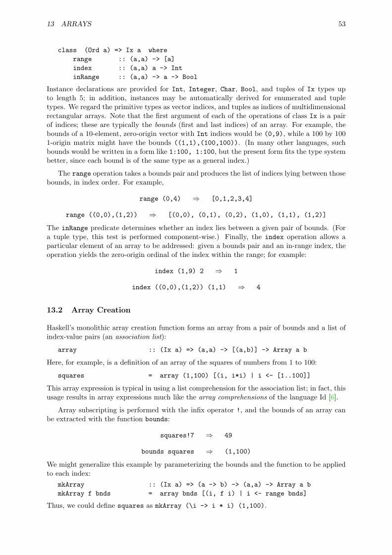
13 ARRAYS 53

class (Ord a) => Ix a whererange :: (a,a) -> [a]index :: (a,a) a -> IntinRange :: (a,a) -> a -> Bool

Instance declarations are provided for Int, Integer, Char, Bool, and tuples of Ix types upto length 5; in addition, instances may be automatically derived for enumerated and tupletypes. We regard the primitive types as vector indices, and tuples as indices of multidimensionalrectangular arrays. Note that the first argument of each of the operations of class Ix is a pairof indices; these are typically the bounds (first and last indices) of an array. For example, thebounds of a 10-element, zero-origin vector with Int indices would be (0,9), while a 100 by 1001-origin matrix might have the bounds ((1,1),(100,100)). (In many other languages, suchbounds would be written in a form like 1:100, 1:100, but the present form fits the type systembetter, since each bound is of the same type as a general index.)

The range operation takes a bounds pair and produces the list of indices lying between thosebounds, in index order. For example,

range (0,4) ⇒ [0,1,2,3,4]

range ((0,0),(1,2)) ⇒ [(0,0), (0,1), (0,2), (1,0), (1,1), (1,2)]

The inRange predicate determines whether an index lies between a given pair of bounds. (Fora tuple type, this test is performed component-wise.) Finally, the index operation allows aparticular element of an array to be addressed: given a bounds pair and an in-range index, theoperation yields the zero-origin ordinal of the index within the range; for example:

index (1,9) 2 ⇒ 1

index ((0,0),(1,2)) (1,1) ⇒ 4

13.2 Array Creation

Haskell’s monolithic array creation function forms an array from a pair of bounds and a list ofindex-value pairs (an association list):

array :: (Ix a) => (a,a) -> [(a,b)] -> Array a b

Here, for example, is a definition of an array of the squares of numbers from 1 to 100:

squares = array (1,100) [(i, i*i) | i <- [1..100]]

This array expression is typical in using a list comprehension for the association list; in fact, thisusage results in array expressions much like the array comprehensions of the language Id [6].

Array subscripting is performed with the infix operator !, and the bounds of an array canbe extracted with the function bounds:

squares!7 ⇒ 49

bounds squares ⇒ (1,100)

We might generalize this example by parameterizing the bounds and the function to be appliedto each index:

mkArray :: (Ix a) => (a -> b) -> (a,a) -> Array a bmkArray f bnds = array bnds [(i, f i) | i <- range bnds]

Thus, we could define squares as mkArray (\i -> i * i) (1,100).

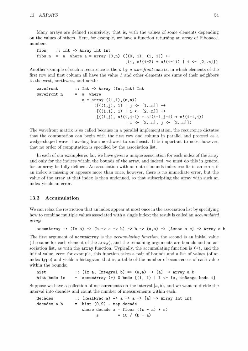
13 ARRAYS 54

Many arrays are defined recursively; that is, with the values of some elements dependingon the values of others. Here, for example, we have a function returning an array of Fibonaccinumbers:

fibs :: Int -> Array Int Intfibs n = a where a = array (0,n) ([(0, 1), (1, 1)] ++

[(i, a!(i-2) + a!(i-1)) | i <- [2..n]])

Another example of such a recurrence is the n by n wavefront matrix, in which elements of thefirst row and first column all have the value 1 and other elements are sums of their neighborsto the west, northwest, and north:

wavefront :: Int -> Array (Int,Int) Intwavefront n = a where

a = array ((1,1),(n,n))([((1,j), 1) | j <- [1..n]] ++[((i,1), 1) | i <- [2..n]] ++[((i,j), a!(i,j-1) + a!(i-1,j-1) + a!(i-1,j))

| i <- [2..n], j <- [2..n]])

The wavefront matrix is so called because in a parallel implementation, the recurrence dictatesthat the computation can begin with the first row and column in parallel and proceed as awedge-shaped wave, traveling from northwest to southeast. It is important to note, however,that no order of computation is specified by the association list.

In each of our examples so far, we have given a unique association for each index of the arrayand only for the indices within the bounds of the array, and indeed, we must do this in generalfor an array be fully defined. An association with an out-of-bounds index results in an error; ifan index is missing or appears more than once, however, there is no immediate error, but thevalue of the array at that index is then undefined, so that subscripting the array with such anindex yields an error.

13.3 Accumulation

We can relax the restriction that an index appear at most once in the association list by specifyinghow to combine multiple values associated with a single index; the result is called an accumulatedarray:

accumArray :: (Ix a) -> (b -> c -> b) -> b -> (a,a) -> [Assoc a c] -> Array a b

The first argument of accumArray is the accumulating function, the second is an initial value(the same for each element of the array), and the remaining arguments are bounds and an as-sociation list, as with the array function. Typically, the accumulating function is (+), and theinitial value, zero; for example, this function takes a pair of bounds and a list of values (of anindex type) and yields a histogram; that is, a table of the number of occurrences of each valuewithin the bounds:

hist :: (Ix a, Integral b) => (a,a) -> [a] -> Array a bhist bnds is = accumArray (+) 0 bnds [(i, 1) | i <- is, inRange bnds i]

Suppose we have a collection of measurements on the interval [a, b), and we want to divide theinterval into decades and count the number of measurements within each:

decades :: (RealFrac a) => a -> a -> [a] -> Array Int Intdecades a b = hist (0,9) . map decade

where decade x = floor ((x - a) * s)s = 10 / (b - a)

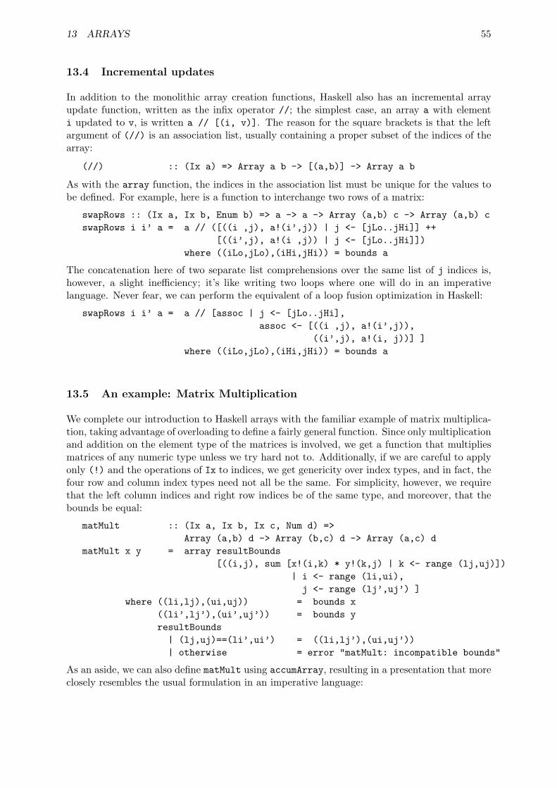
13 ARRAYS 55

13.4 Incremental updates

In addition to the monolithic array creation functions, Haskell also has an incremental arrayupdate function, written as the infix operator //; the simplest case, an array a with elementi updated to v, is written a // [(i, v)]. The reason for the square brackets is that the leftargument of (//) is an association list, usually containing a proper subset of the indices of thearray:

(//) :: (Ix a) => Array a b -> [(a,b)] -> Array a b

As with the array function, the indices in the association list must be unique for the values tobe defined. For example, here is a function to interchange two rows of a matrix:

swapRows :: (Ix a, Ix b, Enum b) => a -> a -> Array (a,b) c -> Array (a,b) cswapRows i i’ a = a // ([((i ,j), a!(i’,j)) | j <- [jLo..jHi]] ++

[((i’,j), a!(i ,j)) | j <- [jLo..jHi]])where ((iLo,jLo),(iHi,jHi)) = bounds a

The concatenation here of two separate list comprehensions over the same list of j indices is,however, a slight inefficiency; it’s like writing two loops where one will do in an imperativelanguage. Never fear, we can perform the equivalent of a loop fusion optimization in Haskell:

swapRows i i’ a = a // [assoc | j <- [jLo..jHi],assoc <- [((i ,j), a!(i’,j)),

((i’,j), a!(i, j))] ]where ((iLo,jLo),(iHi,jHi)) = bounds a

13.5 An example: Matrix Multiplication

We complete our introduction to Haskell arrays with the familiar example of matrix multiplica-tion, taking advantage of overloading to define a fairly general function. Since only multiplicationand addition on the element type of the matrices is involved, we get a function that multipliesmatrices of any numeric type unless we try hard not to. Additionally, if we are careful to applyonly (!) and the operations of Ix to indices, we get genericity over index types, and in fact, thefour row and column index types need not all be the same. For simplicity, however, we requirethat the left column indices and right row indices be of the same type, and moreover, that thebounds be equal:

matMult :: (Ix a, Ix b, Ix c, Num d) =>Array (a,b) d -> Array (b,c) d -> Array (a,c) d

matMult x y = array resultBounds[((i,j), sum [x!(i,k) * y!(k,j) | k <- range (lj,uj)])

| i <- range (li,ui),j <- range (lj’,uj’) ]

where ((li,lj),(ui,uj)) = bounds x((li’,lj’),(ui’,uj’)) = bounds yresultBounds

| (lj,uj)==(li’,ui’) = ((li,lj’),(ui,uj’))| otherwise = error "matMult: incompatible bounds"

As an aside, we can also define matMult using accumArray, resulting in a presentation that moreclosely resembles the usual formulation in an imperative language:

14 THE NEXT STAGE 56

matMult x y = accumArray (+) 0 resultBounds[((i,j), x!(i,k) * y!(k,j))

| i <- range (li,ui),j <- range (lj’,uj’)k <- range (lj,uj) ]

where ((li,lj),(ui,uj)) = bounds x((li’,lj’),(ui’,uj’)) = bounds yresultBounds| (lj,uj)==(li’,ui’) = ((li,lj’),(ui,uj’))| otherwise = error "matMult: incompatible bounds"

We can generalize further by making the function higher-order, simply replacing sum and(*) by functional parameters:

genMatMult :: (Ix a, Ix b, Ix c) =>([f] -> g) -> (d -> e -> f) ->Array (a,b) d -> Array (b,c) e -> Array (a,c) g

genMatMult sum’ star x y =array resultBounds

[((i,j), sum’ [x!(i,k) ‘star‘ y!(k,j) | k <- range (lj,uj)])| i <- range (li,ui),

j <- range (lj’,uj’) ]where ((li,lj),(ui,uj)) = bounds x

((li’,lj’),(ui’,uj’)) = bounds yresultBounds| (lj,uj)==(li’,ui’) = ((li,lj’),(ui,uj’))| otherwise = error "matMult: incompatible bounds"

APL fans will recognize the usefulness of functions like the following:

genMatMult maximum (-)genMatMult and (==)

With the first of these, the arguments are numeric matrices, and the (i , j )-th element of the resultis the maximum difference between corresponding elements of the i -th row and j -th column ofthe inputs. In the second case, the arguments are matrices of any equality type, and the result isa Boolean matrix in which element (i , j ) is True if and only if the i -th row of the first argumentand j -th column of the second are equal as vectors.

Notice that the element types of genMatMult need not be the same, but merely appropriatefor the function parameter star. We could generalize still further by dropping the requirementthat the first column index and second row index types be the same; clearly, two matrices couldbe considered conformable as long as the lengths of the columns of the first and the rows of thesecond are equal. The reader may wish to derive this still more general version. (Hint: Use theindex operation to determine the lengths.)

14 The Next Stage

A large collection of Haskell resources is available on the web at haskell.org. Here you willfind compilers, demos, papers, and much valuable information about Haskell and functional pro-gramming. Haskell compilers or interpreters run on almost all hardware and operating systems.The Hugs system is both small and portable – it is an excellent vehicle for learning Haskell.

15 ACKNOWLEDGEMENTS 57

15 Acknowledgements

Thanks to Patricia Fasel and Mark Mundt at Los Alamos, and Nick Carriero, Charles Consel,Amir Kishon, Sandra Loosemore, Martin Odersky, and David Rochberg at Yale University fortheir quick readings of earlier drafts of this manuscript. Special thanks to Erik Meijer for hisextensive comments on the new material added for version 1.4 of this tutorial.

References

[1] R. Bird. Introduction to Functional Programming using Haskell. Prentice Hall, New York,1998. 1

[2] A.Davie. Introduction to Functional Programming System Using Haskell. Cambridge Uni-versity Press, 1992. 1

[3] P. Hudak. Conception, evolution, and application of functional programming languages.ACM Computing Surveys, 21(3):359–411, 1989. 1

[4] Simon Peyton Jones (editor). Report on the Programming Language Haskell 98, A Non-strict Purely Functional Language. Yale University, Department of Computer Science TechReport YALEU/DCS/RR-1106, Feb 1999. 1

[5] Simon Peyton Jones (editor) The Haskell 98 Library Report. Yale University, Departmentof Computer Science Tech Report YALEU/DCS/RR-1105, Feb 1999. 1

[6] R.S. Nikhil. Id (version 90.0) reference manual. Technical report, Massachusetts Institute ofTechnology, Laboratory for Computer Science, September 1990. 13.2

[7] J. Rees and W. Clinger (eds.). The revised3 report on the algorithmic language Scheme.SIGPLAN Notices, 21(12):37–79, December 1986. 10

[8] G.L. Steele Jr. Common Lisp: The Language. Digital Press, Burlington, Mass., 1984. 10

[9] P. Wadler. How to replace failure by a list of successes. In Proceedings of Conferenceon Functional Programming Languages and Computer Architecture, LNCS Vol. 201, pages113–128. Springer Verlag, 1985. 8.3

[10] P. Wadler. Monads for Functional Programming In Advanced Functional Programming ,Springer Verlag, LNCS 925, 1995. 9, 9.3

a gentle introduction to haskell 98 · haskell programming experience, and cannot be avoided. 2...

Documents