A GEOMAGNETIC INDUCTION STUDY

IN THE

NORTH EAST OF TASMANIA

by

NAZHAR BUYUNG

Submitted in partial fulfilment

of the requirements for the

degree of Master of Science

UNIVERSITY OF TASMANIA

HOBART

1980

ABSTRACT

During the period in between February 1978 until October 1979,

a geomagnetic variation study by means of eleven temporary field

stations has been conducted covering the area of Launceston quadrangle,

Tasmania Geological Atlas Series, sheet SK 55-4, scale 1 : 250 000.

The study area is situated between latitude 41 °00 and 41 °45 south and

between longitude 146 ° 15 and 148 °00 east, with a total area of about

12 700 sq. km .

The aim of this study is to record and analyse the behavior of

geomagnetic variations which are related to lateral changes of elect-

rical conductivity structure.

The coast effect similar to the one that was established in

Hobart ( Parkinson, 1962 ) is found in this area for longer periods

greater than 64 minutes. And an anomalous local high conductivity

zone is indicated by the directions of induction vectors at periods

less than or equal to 48 minutes. This anomalous conductive zone is

interpreted as caused by deep lateral variation of conductivity of

sedimentary rocks ( a-= 0.54 x 10-1 S.m-1 ) with ages between Cambrian

and younger and Devonian granodiorite (a- = 0.54,x 10-3 S.m-1 ), both

being covered by surface high conductive layer ( a - = 0.11 S.m-1 ) that

extends from east of Deloraine to west of Scottsdale.

The occurence of a mineralized zone between Nabowla,Scottsdale

and Tayene agrees with the direction of induction vectors at those

stations.

LIST OF CONTENT'S

ABSTRACT

CHAPTER I GEOMAGNETIC VARIATION STUDIES IN GENERAL 1

I-1 LATERAL CONDUCTIVITY DISTRIBUTION 1

1-2 INDUCTION VECTORS AROUND TASMANIA 3 1-3 CONDUCTIVITY VALUES OF ROCKS 5

CHAPTER II LOCAL GEOMAGNETIC VARIATION STUDIES IN

NORTH EAST TASMANIA 7 II-1 GEOMAGNETIC VARIATION MEASUREMENT AND

CALIBRATION 11

11-2 DATA REDUCTION 13

11-2-1 FOURIER ANALYSIS 15

11-2-2 COHERENCY 17

11-2-3 DETERMINATION OF TRANSFER FUNCTIONS

A AND B 19

CHAPTER III INDUCTION VECTORS ANALYSIS AND INTERPRETATION 25

III-1 INDUCTION VECTORS 25

111-2 SELECTION OF DATA FOR INTERPRETATION 35 111-3 GEOLOGICAL INFLUENCE IN DESIGN OF MODELS 41

III-4 METHOD OF INTERPRETATION 42

111-5 INTERPRETATION OF STRUCTURE 48

CHAPTER IV CONCLUSIONS 50

ACKNOWLEDGEMENTS 51

REFERENCES 52

PLATE I SUBSTORM EVENTS 56

PLATE II TRANSFER FUNCTIONS PLOTS 62

PLATE III MODEL AND COMPUTED SURFACE VALUES 74 APPENDIX I TRANSFER FUNCTIONS VALUES A AND B 82

' APPENDIX II AZIMUTHS AND LENGTHS OF THE

INDUCTION VECTORS 103

APPENDIX III SITE OF OBSERVATION STATIONS

AND MAP REFERENCES NUMBER 106

This thesis contains no material which has been accepted for

the award of any other degree or diploma in any University

and to the best of my knowledge and belief, contains no copy

or paraphrase of material previously published or written

by another person, except where due reference is made in the

text of this thesis.

Nazhar Buyung

March.7, 1980

' . ~ -

' I· I I

I I

I I

I I I j.

I 1

I :

l I l . !

I I

I I· I

I l

! ! l :. ~ . !. ;

'

_,: .•· :

i - : ....... ·

·· .. _

.,... .. \ ·- .... ~ .....

0

Canberra

.. ·. f ··.

t ··-··- ·---------~----- :_. ___ ··-·-· ---- ~-- -------· . -·--

Fig._ 1 Geographical location map of Tasmania and bathymetric

contours around the south east of Australia.

·l

Chapter I

MAGNETIC VARIATION STUDIES IN GENERAL

Many reports about the vertical conductivity distribution inside

the earth have been published from the analysis of gemagnetic variati-

ons, since Schuster (1908) and Chapman (1919) recognized that there is

a region of higher conductivity at a depth of some hundreds of kilome-

ters inside the earth. The vertical conductivity distribution has be-

en refined by the work of many researchers such as Lahiri and Price

(1939), McDonald and Cantwell (1957) and Banks (1969).

The global average model suggests that conductivity value between

depths of 0 and 400 kms would not exceed 0.10 S.m -1 but the existence

of material with conductivity in excess of that value has been report-

ed. It is usually suggested that this is related to some factor such

as saline water filled sediments, zone mineralization, or high heat

flow. For greater depth, high conductivity anomalies are normally as-

cribed to partial melting of magma in the upper mantle (Banks, 1979).

I-1 LATERAL CONDUCTIVITY DISTRIBUTION

The lateral conductivity distribution is well indicated by the

direction of induction vectors. The induction vector is a 2-D vector

(A,B) where A and B are transfer functions describing the behavior of

the vertical component as a function of the horizontal components.

Its modern definition is given by

Z A.X B:Y

where are (complex) Fourier transforms of the field components, are

and A and B are chosen to minimize C. In general they vcomplex numbers,

so we must deal with both a real and imaginary induction vector.

After the invention of induction vector by Parkinson (1962) and

independently by Wiese (1962), the study of electrical conductivity

distribution grew rapidly. Induction vectors introduced by Parkinson

differ from those of Wiese; the direction of the former is toward

higher conductivity, while the one introduced by Wiese is away from it.

Throughout this paper the induction vectors pointing toward conductivi-

ty anomaly were adopted.

Al]. over the world many areas have been intensively studied.

Lilley(1975) and Adam (1976) summarized some of the areas studied to

date. The response from all of those studies, have brought to light

the behavior of magnetic variations at some particular areas. For some

areas by noticing the characteristic of the directions and lengths of

the induction vectors and the locality of the station observations con-

cerned, the lateral effect of conductivity could be categorized into

one of known effects such as coast, island peninsula and strait

effects. Al]. of these effect are related to the influence of induced

electric current flowing in the sea water and in fact are frequency

dependent.

One classical example of the coast effect is shown on the induction

vectors plotted around Australia and the region surrounding ( Parkinson,

1962 ). All of the vectors point toward the adjacent deep ocean and

perpendicular to the coast line. Other reports of the coast effect

are in California by Schmucker (1963) and in Canada by Hyndman (1963)

and by Lambert and Caner (1965).

On relatively uniform conductivity distributions, the coast effect

causes the length of the induction vectors to be longer at stations on

coast line and gradually to decrease inland. Longer induction vectors

at inland stations compared to the one at coast line, indicate the land

area is conductively anomalous.

The coupling between mantle and ocean conductivities weakens the

electrical current intensity flowing in the ocean ( Honkura, 1971), and

will affect the bahavior of the vectors effected by the ocean.

An exceptional case of the induction vectors at a coast line is

found in Peru, where the land anomaly is so strong that it causes the

coast effect to vanish ( Schmucker, 1969 and Aldrich et al., 1972 ).

The island effect differs slightly from the coast effect, since

it is best seen at short period variations. Extensive studies about

this effect have been done at Oshima (Sasai, 1967, 1968), Oahu (Klein,

1972), Miyake-jima (Honkura, 1971) and Hawaii (Klein, 1971). All in-

duction vectors are characterized by the directions toward the sea

away from the island.

The peninsula effect is considered as combination of coast and

island effects which sometimes causes the amplitude of vertical vari-

ation (AZ) to be greater than the horizontal variations (AH and AD),

although the coast effect itself sometimes also does this.

The strait effect is simply indicated by the direction of induc-

tion 4ectors on lands at both side of the strait point toward the 7115

strait, the* is caused by the induced electric current being channeled

through the conductive strait.

1-2 INDUCTION VECTORS AROUND TASMANIA

Four induction vectors had already been established in Tasmania,

before this study started in early 1978 (see figure 2). The induction

vector at Hobart is one of the few induction vectors around the

Australian coastal region. It was determined from bay type and similar

geomagnetic fluctuations at period of 40 minutes. The direction of the

vector is toward the deep ocean in the south east.

Three stations on the north coast of Tasmania, Bridport, Devonport

and Smithton are part of magnetometer array stations at the south east

Australia done by Lilley (1973-1974). The vectors are for periods of

1

100 km

1.0 . I

mal

- 4 -

5 - 20 minutes. The directions of induction vectors at Bridport and

Devonport are toward a point slightly north of the line joining them.

An indication of electric current with a direction northwest to

south east passing -

Figure 2 : Induction vectors around Tasmania. Hobart vector

is for 40 minutes period, and Smithton, Devonport

and Bridport vectors are for 5 - 20 minutes period.

• Lilley ( 1973 - 1974 )

0 Parkinson ( 1962 )

- 5 -

through conductive zone inland could be assumed.

To understand the behavior of induction vectors and to interpret the

possible conductivity structure of this area forms the objective of

this study.

1-3 CONDUCTIVITY VALUES OF ROCKS

The important parameter involved in interpreting the subsurface

structure derived from the geomagnetic variations is conductivity, i.e

reciprocal of resistivity. Its unit in electromagnetic unit is emu,

and in MKS units it is mho.m-1 or Siemen.m-1 .

-1 1 Siemen.m is equal to 10-11 emu.

Measurement of the conductivity value of rock in the laboratory was

discussed in detail by Scott et al(1967) and Duba (1978).

The conductivity of a cylindrical sample can be simply calculated

through measurement of its resistance in ohm, by the relation ;

R = 07 A

where R is the resistance in ohm, L is the length of sample in meter,

c is the conductivity and A is the surface area in m 2 .

Laboratory results of conductivity _values of rocks after being satu-

rated in various saturants such as tap water ( or= 0.95 x 10-2 S.m-1

)

distilled water ( o- = o.44 x 10-3 s.m-1 ) and 0.1 M NaC1 done by

Duba (1978) are tabulated below.

TABLE 1 (after DUBA, 1978)

Lithology Saturated in

Distilled water Tap water

( S.m-1 ) ( S.m-1 )

Kayenta sandstone 0.44 x 10-2 0.18 x 10-2 (Triassic)

St. Peters sand- 0.23 x 10-2 stone (Ordovician) 0.11 x 10-2

-3 Indiana limestone 0.56 x 10- 0.19 x 10 3 (Upper Ordovician)

0.1 M NaCl

( S.m-1 )

0.86 x 10-1

0.43 x 10-1

0.12 x 10-1

cont'd

Lithology

Nugget sandstone

Westerly granite (Upper Permian)

Saturated in

Distilled water Tap water

( S.m-1 ) ( S.m-1 )

0.52 x 10-2 0.30 x 10-2

0.11 x i0 x 10-4

0.1 M NaCl

( S.m-1 )

0.98 x 10-2

0.58 x 10-3

Limestone and granite are known for their low porosity, thus the

low conductivities after saturation are expected.

Measurement of conductivity values of various rocks from the study

area were also done. The samples in the form of cylinders were clam-

ped as five layers sandwiches (electrode - blotter - sample - blotter

- electrode), and their resistances were measured using a Potentio-

metric Voltmeter ( flPORTAMETRIC" PVB 300, serial no. 430057 ).

To make a good contact between the copper electrode and sample, wet

blotting paper saturated with CuSO4 solution was used. The results

of measurement are tabulated in TABLE 2.

TABLE 2

MEASURED CONDUCTIVITY VALUES

Lithology

Clayey sand

Loose sand

Sandstone

Basalt porous

Basalt compact

Not saturated

-1 ) ( S.m

0.26 x 10-2

0.33 x 10-2

0.59 x 10-2

0.66 x 10 -4

0.51 x 10

Saturated in

tap water - ( S.m 1 )

x 10 -3 0.77 x 10

Saturated in

brackish water

( S.m-1 )

-

-

-

x 10-1

0.76 x 10-3

. Granodiorite 0.54 x 10 x lo-2 0.25 x 10-2

Knowledge about measured conductivity values of rocks will give

some help to generalize the conductivity distribution throughout the

area. But since the conductivity values of rocks inside the earth are

sensitive to temperature and compactness (related to water content),

interpretation of conductivity structure on this basis need a high

presumption.

-r·

I I

-L-

C;tmpter II

LOCAL GEOMAGNETIC VARIATION STUDIES IN NORTH EAST TASMANIA

The location of the study area is shown in figure 3, and the distri-

bution of the stations in figure 4.

Bass Strait with 200 meters deep sea water separates Tasmania from the

mainland with a distance of about 400 ~s.

Eleven temporary stations were _distributed throughout the area. The

names, abbreviations and geographic coordinates are tabulated on Table 3.

1471boE

.....,_;-------t ··TA S M A N I A· 4o0oos 0 100km . ·

LOCATION MAP OF- SURVEY .AREA

B A S S

_ .... ···' =:·

{ ·~ ........ I

';I

/, .......... --·:.\ '· i ';..Oeloralne . -:'.-········· . . LL..__. _ _.

,·"' .....

.:·········

·· ... ! . .

.. ________ .-. 0 '·· _ ...... l '-·........ p

. -. . . ..... ( \ ··-·-.

...... ;... ...... ..-·· ··-.... ~ . .. ··---······ 0

- 7 -

r (

.li

·· ... \-: .. .:-~

• WJC .•DLR

-4 • 111M 111M44111

• IFIIT

• N•L SCUTUM

- •LLD

0 LAIIICISTS11

• TAY

Figure 4 : Locations

Station

of geomagnetic observation points.

TABLE 3

Abbreviation Latitude Longitude

1. Western Junction WJC 41 °32'45 147°12'24

2. Scottsdale SCD 41 °09 , 47 147°31 , 02

3. Deloraine DIR 41 °31'30 146°39 , 34

4. Rosevale RSV 41 °25 , 39 146°55'58

5. -Lilydale LID 41 °15 1 47 147°13'27

6. Nabowla NBL 41 °10 , 34 147°16'58

7. Forester FRT 41 °04 , 44 147°40 , 45

8. West Frankford WFR 41 °18'33 146°42 1 56

9. Pipers River PPR 41 °07 , 18 147°06 1 40

10. Beechford BFR 41 °01 , 58 146°58'02

11. Tayene TAY 41 °21'19 147°27 1 24

Legend

Parts of major Tertiary fault lines (Banks, 1962) d,

Cambrian and younger rock formations

Devonian granite - granodiorite

Siluro Devonian Mathinna Beds

VN1 mg Precambrian rocks

Four stations, WJC, RSV, DLR and WFR are located on the area that

geologically has complicated structure with outcropped rocks ranging in

age from Precambrian and younger and covered by Tertiary sediments filling

a graben and relatively thin sills of Jurassic Dolerite.

The remaining seven stations, LLD, NBL, SCD, FRT, BFR, PPR and TAY

are located on the area which has relatively simple major geological

distribution of formations of Mathinna Beds and later intrusion of

Devonian granite - granodiorite type. The Mathinna Beds have a thickness

of at least 2 000 meters, but the total thickness is unknown (Banks, 1962).

— 1 0 —

TAMAR GRAVITY SURVEY • STRUCTURAL FEATURES

Fig. 6 Structural features of Tamar area derived from

gravity anomaly (Leaman et al., 1976)

Gravity measurements have also been made over this area during the

period 1971 to 1975 (Longman et al. 1 1971 and Leaman et al.,1976).

Their regional gravity anomaly maps show a regional increase of ano-

maly toward the east that indicates a shallowing of the Moho.

Noticed also that the structural features derived from gravity anoma-

lies (see figure 6) show many cupolas at the area between Nabowla,

Scottsdale and Tayene, that seem to associate with the existence of

mineralization.

- 11 -

II-1 GEOMAGNETIC VARIATION MEASUREMENT AND CALIBRATION

The data of magnetic variations at Western Junction and half of

Scottsdale were recorded using a 3-components Fluxgate magnetometer

known as TOPMAG abbreviated from Tasmania Operation Magnetometer.

The magnetometer has no temperature control. To eliminate the effect

of temperature variation between night and day, the detector was bu-

ried underground. From experience 50 cms of soil on top of the detec-

tor was enough to eliminate the temperature effect.

The magnetic variation data of the rest of the 9 stations and half of

Scottsdale were recorded using a commercial Fluxgate (EDA instrument

FM-100B, serial no. 2117). This magnetometer was put into ,operation

on July 1978. The advantage of this new instrument is the built in

temperature compensator; that means the detector does not have to be

buried.

MAGNETOMETER CALIBRATION

TOPMAG : This magnetometer was calibrated using built in Helmholtz

coils, in the form of two similar coaxial coils separated by a distan-

ce equal to their common radius and carrying current in the same direc-

tion. This formed the calibrating coil system for each component. The

built in coils were tested and calibrated against a standard Helmholtz

coil (Askania, serial no. 582047). It was found that the built in coils

have the following values : D = 27.5 nT/mA

H = 28.5 nT/mA

Z = 26.7 nT/mA

By applying known values of current into the coils, and measuring the

needle deflection at chart recorder, the magnetometer sensitivity can

be calibrated. The sensitivity values are :

D = 4.13 nT/mm

H = 4,.28 nT/mm, Z = 4.01 nT/mm

12-

FM 100 B FLUXGATE MAGNETOMETER

The value of 10 Volts output from magnetometer is specified by

manufacture as more less equal to 1 000 nT ( manual FM 100B ).

To find the accurate value, a clibration was done using a square

coils. The specific parameters of this square coils are ; each coils

system has four separated coil, where the outer coils have more number

of turns of wire than the inner coils, as specified below.

Vertical field coils : Z outer coils

Z inner coils

a = 0.27 m,

a = 0.27 m,

N =

N =

140,

60,

b/a = 1

b/a = 0.26

Horizontal field coils: H outer coils

H inner coils

a = 0.25 m,

a = 0.25 m,

N =

N =

70, b/a = 1

30, b/a = 0.26

where; a is half distance between the two outer coils, and b is half

distance between the two inner coils.

The value of magnetic field intensity and current ratio, resulting if a

current (I) is applied to the coils ( 4 square coils ) is determined as : A ,U4 a2

= X X in Tesla/Ampere 7r (a2-1-132 ) V 2a2+b2 All the parameters are known values. Thus the sensitivity of this square

coils in term of nT/mA can be obtained.

The vertical Z field is 471.1 nT/mA

The horizontal H field is 254.4 nT/mA

The detector of particular component to be measured then oriented

parallel to the magnetic field direction of the coils, and put right in

the middle. By applying a known current value into the coils, the out-

put voltage from magnetometer can be measured. From measurements were

found the sensitivity-value of magnetometer for each component as below :

H component = 92.2 nT/Volt

D component = 90.7 nT/Volt

Z component = 90.8 nT/Volt

- 13 -

11-2 DATA REDUCTION

The object of data reduction is to calculate the complex numbers

of transfer function values A and B from the group of discrete events of

three components of geomagnetic storms, that fit into the statistical

relation : AZ = Alai 4- iLLA) at a particular frquency.

AZ I AH and AD are the amplitude variations of geomagnetic components

on the directions vertical down, magnetic north and magnetic east respect-

ively.

The particular events that were of interest in this study are the

substorm type. Examples of the substorms are shown in Plate I.

It can be seen that the single event, which in particular so called bays

provide an excellent signal which clearly stands out from the general

background activity.

SAMPLING

Data in the analog forms which were recorded using two Rustrak type

288 and one Multiscript 3, were sampled partly by hand and partly by semi

automatic scaler.

Hour marks are 2.5 cms apart and the full scale of the chart paper is

equal to about 240 nT.

Because of the time resolution ( 2.4 minutes/mm ) and the blurred

image of some of traces, hand digitized samples are considered reliable

only at 6 minutes intervals, allowing analysis of periods greater than or

equal to 12 minutes.

Sampling using the scaler gives results that are consistent with those

done by hand, except that the 'sample intervals can be shorter.

The output of the scaler is converted to digital form and fed into

the computer. Values in between the scaled points are internally inter-

lated. The relative values of every component (in nT) and at particu-

a) H polarity

b) D polarity

Z polarity

•

[IN. A ,

Figure 7

lar event were processed through INTERDATA 67/16 Computer and output

in the form of 8 hole binary code in _paper tape as a preparation for

Fourier analysis.

A very important thing to notice is the polarity of the data being

sampled, which means which is the direction of magnetic north, magnetic

east or vertically down. These polarities are used to determine the di-

rection of the induction vectors.

Determination of those polarities were done by the help of a permanent

magnet being put at some distance from the detector. After the detectors

have been set up with H detector pointing north, D detector pointing east

and Z detector vertical, polarities are determined as follows :

By applying the permanent magnet ( N pole

to north direction ) parallel to detector,

the direction of needle movement at re-

corder indicates south direction ( i.e

negative is south on chart in figure 7a ).

By applying the permanent magnet ( N pole

to east direction ) in line with the de-

tector, the direction of needle movement

at recorder indicates east direction ( i.e

positive is east on chart in figure 7h ).

By applying the permanent magnet ( N pole

points up ) vertically parallel to detec-

tor, the direction of needle movement in-

dicates down direction ( i.e positive down

on chart in figure 7c ).

- 1 5

II-2-1 FOURIER ANALYSIS

Before the sampled time series of data were transformed into the

frequency domain, the amplitude data were calculated as the deviation

from a straight line connecting the beginning and the end of the event.

Also the mean of the first and the last few numbers were padded with

zeros to 2n values.

The calculation into the frequency domain was done in the INTERDATA

67/16 Computer, using the Fast Fourier Transform subroutine that already

exists in the computer library, and output in the forms of Cosine ( C )

and Sine ( S )functions of Fourier coefficients of various frequencies

ranging from the first harmonic to the one that has period twice the

sampling interval, into paper tape as data which are prepared for the

next computing of the transfer function values A and B.

Example of computed amplitude and phase spectrums of H, D and Z

components plotted against periods are shown in figure 8.

The relations between amplitude and phase spectrums with the Cosine

( C ) and Sine ( S ) functions are :

Amplitude (co) = ( C 2 +

Phase (co = tan -1

Figure 8 is the plotted spectrums of the event at Rosevale for six

6 28 hours from 161 1 6 to 22in'September:1978.

I I I. I ! I

j I I '

I I.

I I

40

30

10

Amplitude . Phase H.

z

48 32 24 18 13 In minute•

Figure 8

- 17 -

11-2-2 COHERENCY

A check of coherency between the vertical and the horizontal com-

ponents was done using the equation ( Kanasewich, 1973 ) that was modi- 2

fied as : C = B*> <41 2 >.< 1E1 2 >

where Z is the Fourier transform of Z component.

= H • cos A + D • sin Q ( H and D are the Fourier transforms

of H and D components respectively and Q is the azimuth.

- The asterisk * indicates the complex conjugate of complex

number concerned.

- The brackets< )indicate averaging over all events. Notice

that averaging was done over events at constant period, not

over the adjacent periods.

Expected value for C is close to one if Z is controlled by B. The

closer it is to one the more closely related are the two processes at

-particular period.

Coherencies were calculated for all values of G. The maximum

values and the azimuth of the induction vectors are shown in Table 4.

The coherency values at periods 2k,.32 and 48 minutes appear quite

good at all stations, except values -at 48 and 24 minutes at Scottsdale,

and value at 48 minutes at Forester. The direction of Induction vectors

with relatively relatively amemamma value,. generally coincide with the direction of

either the real or imaginary induction vector whichever is larger.

The coherency values calculated between magnetic component are

generally lower than between e.g E and H. in magnetotellurics. 7

For longer periods, the azimuth A of maximum ICI mostly coincides

with the directions of the imaginary induction vectors, while at short

periods it seem to associate with the real one.

68°

88°

112°

134°

152°

-1 °

, -162°

600

dMIP

88°

-76°

129°

-55°

149°

96 1800 0.77

64 - a=

48 185° 0.76

32 200 0.82

24 195° 0.75

16 300 0.84

13 195° 0.73

1600 0.78

1800 0.71

1900 0.74

1900 0.93

1900 0.92

15° 0.47

300 o.4o

-137° 330° o.46 -120° - 340° 0.70 -132°

-121 °

-109°

-71 °

-137° -33°

330° 0.83

340° 0.79 190° 0.70

3500 0.62

200° 0.39 -10

-122°

-131 ° 20

-154°

- 18 -

TABLE 4

THE MAXIMUM VALUES AND PHASES OF COHERENCY AT VARIOUS PERIODS

DELORAINE ROSEVALE

Period Direct. of ICI Phase Direct, of

Id I Phase in min. Induction of .0 Induction . of C

Vector Vector

LILYDALE . NABOWLA

Period Direct. of IC I ' Phase Direct. of lc I Phase

in min. Induction of C Induction of C Vector Vector

96 340° 0.51 64 - -

48 340° 0.83

32 340° 0.86 24 320° 0.65

16 lo° 0.55 13 250° 0.33

SCOTTSDALE

Phase of C

FORESTER

Period Direction ICI Phase Direct. of ICI in min. of Induction of C Induction

Vector Vector

96 1800 o.49 49° 180° 0.49 750

64 1700 0.75 43° 180° 0.62 41 °

48 320° 0.56 -156° 170° ' 0.29 520

32 320° 0.67 -1140 170° 0.86 81 °

24 170 0.51 290 170° 0.92 85° 13 290° 0.20 -11

o 280° 0.67 6°

i6 190° 0.40 90 290° 0.68 -70°

- 19 -

II-2-3 DETERMINATION OF TRANSFER FUNCTIONS A AND B

Transfer function values A and B are used to determine the in-

duction vector that has been often mentioned earlier. The early method

is by a using polar diagram that was developed by Parkinson ( 1962 ),

where the vector changes of the geomagnetic field tend to lie in a plane,

called by Parkinson as "preferred plane" for the station. AZ AD

Also Sasai (1967) has plotted the ratios of--- against --- for AH AH

geomagnetic variations that have period of 30 minutes and shorter. The

plotted points seem to lie on a straight line. By taking two pairs of va-

lues on that line, and inserting them into the equation :

AZ AD __ = A ± zio • — the transfer functions A and B can AH AH

be found. The two methods that have been discussed above deal only with

the real part of transfer function. For few periods where the three com-

ponents are often out of phase, the calculation of transfer function with

this method becomes more complicated.

For more valid treatment and calculation with wide range of frequency,

the determination of transfer functions that was developed by Everett and

Hyndman (1967) was used. The records which contain geomagnetic activity

( e.g substorm events ) were selected and Fourier coefficients were obtained

for the north, east and vertical components.

For each station a group of values at particular frequency thus

obtained, and these values then were used to find the best fit to the

equation : Z A . H . All of transform values consist

of real and imaginary parts. The equations involved in the calculation

are shown as below ( Everett and Hyndman, 1967 ) :

f• E — N x A , B N E X X NE —XR

- 20 -

where : N =H.H , P X 1

= f2D .

X =EH. 1

these values were summed over n events.

The bar above the letters indicates the conjugate of the complex

number concerned. The transfer function values A and B calculated

using this method are tabulated in Appendix 1 , and are plotted against

periods and shown in Plate II.

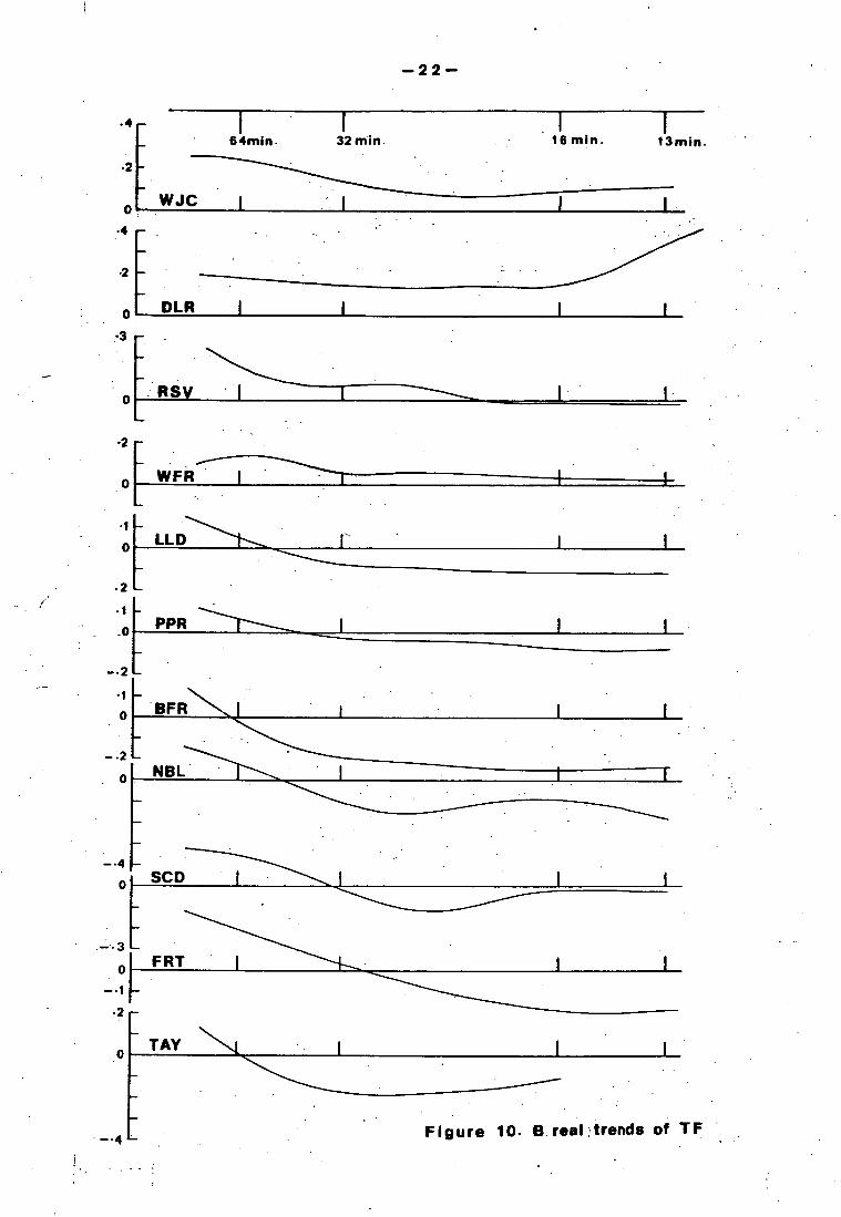
TRENDS OF TRANSFER FUNCTIONS AGAINST PERIODS

There are two clear differences between the transfer function (TF)

values in the areas east and west of the Tamar River, that can be seen

especially from the real parts of the TI'.

The variation trends of TF values plotted against periods are shown

in figures 9 and 10. Most of the stations have TI' trends varying

smoothly with period. The stations with this condition are WJC, DLR,

RSV, WFR, LLD, PPR and FRT ( indicated by full circle in figure 11 4,444.

The trends at SOD and BFR are drawn • relative low un-

certainty at groups of TI' at adjacent periods with small fluctuation

( indicated by half full circles in figure 11). TAY and NBL trends

are difficult to obtain for they have big values of uncertainty, es-

pecially at periods in between 16 and 32 minutes at NBL ( see P1 1177,

page 70).

The graphs of trend in figures 19 and 10 show the appearance of

anomalous characteristic of this area. By knowing . that the positive

A of TI' has the north direction, the negative A of TI' has the south

direction, as well as the B of TI' has the east direction for positive

value and west direction-for negative B value of TI', thus by examining

the trends of the graphs in figures '9 and 10 , some informations can

be derived as follows.

1 -•4

SCD

.3-

-

- RSV

.1 LLD

-.2

PP

-.2

BFR

_ . NBL

-.2

Figure 9 A real trends of TF --4

— 21—

•4 -

1

1 64 min. 32 min. 16min. 13min.

-2

WJC

.4 -

-2 -

DLR

13min. 16 min.

•4

2

WJC

64min. 32min.

1 •BFR

Figure 10. B.real trends of TF

—22-

0 [ DLR

—

-

WFR

• 1

PPR

-•2

SCD

2

-.2

-.4

NBL

- 23 -

Figure 11

All of the west side stations at periods shorter than 32 minutes,

have positive A real, and also positive B real (see figures -9 and 10,

except a part of shorter period at RSV, thus the direction of the

induction vectors will be to the north east.

At the east side, the stations LLD NBL I and SCD have negative values

of A real, but other stations such as PPR, BFR, FRT and TAY have posi-

tive values ( fig. 10 ), meanwhile the B real at all stations in this

side of area have negative values at periods less than 32 minutes

( see fig. 10 ). Thus the directions of the induction vectors will be

to the north west at 1TR, BFR, FRT and TA!, and to the south west at

- 24

LLD, NBL and SCD.

By noticing that the west side stations have induction vectors

point to the north east directions, and the east side stations point

to the south west and north west directions. Thus the area in between

east and west stations shows conductivity anomalies.

The detail explanations about informations that can be derived from

induction vectors at various periods will be explained in Chapter III.

Chapter III

• INDUCTION VECTORS ANALYSIS AND INTERPRETATION

III-1 INDUCTION VECTORS

Induction vectors applied in this analysis as has been mentioned

earlier follow the one that was developed by Parkinson (1962), where the

vectors point toward the high conductive zone. The results of calculati-

on are tabulated in Appendix II. All the induction vectors at periods

96, 64, 51, 52, 24, 16 and 13 minutes are shown in figures 12 to 18.

INDUCTION VECTORS FOR PERIODS 64 AND 85 - 96 MINUTES ( Figure 12.13 )

The effect of the coast from the deep ocean to the south east clear-

ly influences the induction vectors at this range of period. Although the

effect can be seen at all of the stations, the west side stations WJC, RSV,

DLR and WFR are more stable in .direction.

At all stations on the east side of the Tamar, as soon as the period

decreases to 64 minutes, there is a slight rotation of the vectors to the

west. This indicate that the effect of deep lateral variations of conduc-

tivity to the west of these stations has started to give some effect.

Notice also that the length of the induction vectors are shorter at the

stations on the north compared than those at the south, indicate the re-& de-

ducing of deep sea effect .02 south east direction.

The centre of the survey area is about 185 kms from the continental

slope. On the basis of average coast effect ( e.g Parkinson and- Jones,

1979 ) a transfer function values between 0.2 and 0.3 would be expected.

The observed average value of transfer in the study area is 0.22.

10 20kMS Period: 85-96 minutes real imaginary 0 0.5

G 1.0 U.V.

— 41000$

•

•

• FRT

WFR

TAY

Launceston !

WJC

— 41o30S

Fig, 12

147000E 147030 E

0 10 20 kms

0.5 1.0 u.v. I . j

1

o •

Period:64minutes

real

A ..... imaginary

— 41o00 S

7 BFR

PPR

cCD

LLD

6,1A1,F,R

/TAY

8&1S,V ED .

Launcest4n — 41

o30S

WJCN

Fig. 13

0

-+

146o30 E 147°30 E 147o00E

_ 28 _

INDUCTION VECTORS FOR PERIOD 48 - 51 MINUTE (Figure 14 ) :

At this period the induction vectors at DLR, WFR and RSV are free

from the influence of the southeast ocean effect that occurs at longer

periods, and the deep local lateral conductivity structure effect domi-

nates.

Induction vectors at LLD, NBL, SCD and FRT still have the same directi-

on as the vectors of longer period.

Explanation for this is possibly another deep seated conductive zone

which occurs south of these stations and that is stronger than the ef-

fects of the known zone along the Tamar.

0 10 20 kms 1 1 PeriOd:48-51 minutes

0.5 1.0 U.V. 1 .

--real Imaginary

• S

5

— 41 °00S

BFR

FRT

.4 PPR

V1N

LLD

1NBL

WFR

TAY

6' RS V

Launceston — 41030S

DLR

147°30 E 146 30 E 147o00 E

Fig. 14

-30-

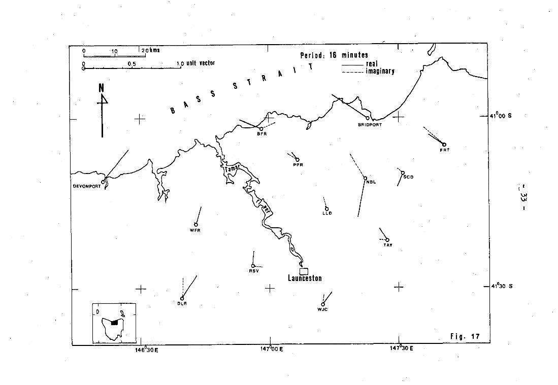
INDUCTION VECTORS FOR PERIODS EQUAL TO AND LESS THAN 32 MINUTES

( Figures 15, 16, 17 and 18 )

The induction vectors throughout this range of period are free

from the south east coast effect, and the remaining factors other

than inland anomaly is the influence of induced field from sea water

in Bass Strait.

Vectors at all stations on the west side clearly show the effect

of the induced electric current near the Tamar graben in the NW - SE

direction, but at period less than 16 minutes those at WFR and RSV ro-

tate nearly to the north direction, where the induced field of Bass Strait

has a dominant influence.

This combination of land anomaly affected by induced fields in

Bass Strait is also shown at FRT I PPR,BFR and Bridport (Lilley,1973-1974).

The direction of induction vectors at NBL, SCD,and TAY at three

ranges of periods ( 324 24 and 16 minutes ) point toward a zone of

mineralization ( see figure 6, page 10 of this paper., Leaman (1976)).

The small lengths and more or less random directions of the

induction vectors at PPR and LLD have been mentioned earlier appear to

be situated right in the middle of a conductive zone.

146 o 30 E 147 °00 E 147 °30 E

Period : 32 minutes real 1

imaginary

, .

kFRT

C D

s'A TAY

— 41 ° 00S

— 41 ° 30S

WJC

Flg. 15

O 10 20 kms

O 0.5 1.0 u.v. O ' • 1 I

Period: 24minutes

real imaginary

41000

k

\ • F

-

RT

b PPR

NBL . 'Co

LLD

TAY

RSV

— 41030

DLR

Launcest9n

WJC

147o00 E 147030E 146o

30E

Fig. 16

10 I 20 kM3

•

0 15 1.0 unit vector Period: 16 minutes real

1 I imaginary

— 41 °00 S BRIDPORT

Ns4NO‘ PRI

PPR

LLD

/NB. L

TAY

RSV

Launceston — 41 o30 S

D LR WJC

Clo 147 30E 147°00 E

Fig. 17

41 o00 S

41°30S

DLR

WJC

Fig. 18 Z-111

'Period : 13 minutes real imaginary

0 10 20 kms

0 0.5 1.0 u.v. • I

TAY

LLD

NBL

17:) -SCD

FRT

PPR

RSV

Launceston

146°30E 147°00E 147°30E

- 35 -

III-2 SELECTION OF DATA FOR INTERPRETATION

Since the induction vectors especially at short periods ( around

32 minutes ) already show an indication of relatively highly conductive

zone that influences the direction of the induction vectors, the possible

electrical conductivity structure that is responsible has to be interpreted.

It has been assumed that the coastal effect of the ocean to the south

east has already vanished at this range of period. Only the induced current

from sea water in Bass Strait remainly influencing the induction vectors at

this local area, and the influence is mainly on the imaginary transfer func-

tion.

The direction of the coast line of this area is about 35 °north of

east. It will be assumed that the predominant conducting zone is linear

and oriented 350 west, of north. This can be justified by the geological

structure and grain of the area, and the direction of induction vectors of

long period west of the Tamar.

At a period of 24 minutes (see figure 16, page 32) the induction

vectors at LLD, NBL and .SCD point toward a conducting zone in a WSW direc-

tion. However the random directions at other stations on this east side

show that this area has complicated conductivity structure.

:Induced electric currents in the pressumed. conducting zone, with a

trend NNW-SSE, cause magnetic field vectors in the.direction 350 north

of east.-.This is parallel to the coastline and perpendicular to the

. regional structure of geology as well as the direction of the conducting

zone. The data used in a two-dimensional interpretation are the components

of the induction vectors projected onto a line bearing 350 north of east.

The stations used are those along the traverse from DLR to FRT.

Considering the projections of. vectors onto a line bearing 35 °north

of east is equivalent to considering a "virtual event" in which the hori-

- 36 -

zontal field is linearly polarized in the direction E 350 N and has

unit amplitude.

The projections of the real and imaginary vectors then indicate

the amplitudes of the in:Phase and out of phase parts of the vertical

field.

Over a wide range of frequencies the imaginary transfer function

vectors tend to lie in fairly uniform direction ( between N and NW ),

and vary in amplitude rather than direction. This is shown in figures

in Plate II, by the imaginary parts of A and B appearing as mirror

images of each other.

The imaginary transfer function vectors seem to be controlled by

induction in the shallow water of Bass Strait, and only the real transfer

function vectors are controlled by conductivity variations on land.

For these reasons only the real part of the transfer function will be

taken more attention in the interpretation of inland anomaly. The con-

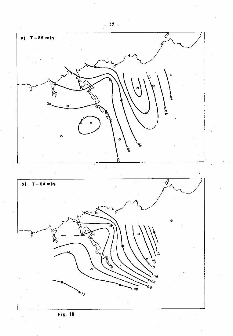
tour maps. of the observed vector components at periods of 85 - 96, 64,

48, 32, 24 and 16 minutes are shown in figures 19 to 21.

At all periods these contour maps show that there is an approximat-

ely two 'dimensional conductivity structure on the west side, while on

the east side a more complex structure is involved. A possible reason

for the complicated structure of conductivity in the area to the east

is a complicated boundary between the granite - granodiorite mass and

the thick sedimentary Mathinna Beds. This would involve an edge .effect

between the low conductive igneous rocks and high conductive sedimentary

rocks.

The observed vector components that will be used as surface field

observations for the interpretation are shown in figure 22. These va-

lues then have to be fitted to the calculated values from models of

conductivity structure.

-37-

Fig. 19

- 38 -

Figure =)20

•I6 #.1 2

T -, 16 min.

-.08

* -08

- 39.--

Fig. 21

— OA

0.2

16 min.

— 0.3

— 0.2

24 min.

— 0.2

— 0.3

^

0

0

85 min.

51 min.

— 0.3

— 0.2

4— 0.3

— 0.2

- 4-o

— 0.2 0

DLR RSV

LLD NBL SCD FRT I I

Figure 22

-

•-

111-3 GEOLOGICAL INFLUENCE IN DESIGN OF MODELS

On the basis of magnetic field variations alone, the distribution

of lateral conductivity that fits the field observation in this region

consists simply of a high conductive zone lying between Deloraine and,

Scottsdale. This follows from the high values of the components of

transfer functions with positive value ( e.g +0.30 for 32 minutes period

at Deloraine ), and gradually decreasing to east - northeast direction

and reaching zero around Lilydale, and becoming high negative at Scottsdale

( e.g -0.16 for 32 minutes period ), and toward Forester the value increase

again.

Because the geology shows that this region consists of several

major rock formations which have clear surface boundaries, the surface

distribution of formation needs to be taken into consideration in the in-

terpretation of magnetic variations.

The surface distribution of rock formations on the profile Deloraine

Forester basically follows the general distribution of major rock forma-

tions that dominantly cover this area ( see figure 5, page 9 ). From

southwest to northeast there is Precambrian basement at southwest of

Deloraine, followed by complicated structure of Cambrian and younger

formations, Mathinna Beds and Permian sedimentary rocks, and granodiorite.

Based on geological evolution, a deep conductivity contrast situ-

ated between Lilydale and Rosevale was assumed. This contrast zone is

consistent with the boundary between contrasting types of Precarboniferous

rocks ( William, 1978 ); those to the east include turbidite type of rocks

as well as micaceous quartzwacke and mudstone sequence, of which the

Mathinna Beds are typical and those to the west are stable shelf deposits

such as interbedded quartz sandstone and mudstone and marine and terres-

trial sediments, quartz sandstone and conglomerate.

-

This boundary may be related to the slight rotation of the induction

vectors to the west for the east side stations for period 64 minutes,

compared to the one with 85 - 96 minutes period.

III-4 METHOD OF INTERPRETATION

The computer program developed by Jones and Pascoe (1971) and

Pascoe and Jones (1972) were used to calculate the response at the Earth's

surface of two-dimensional conductivity structure. The program has been

modified due to errors that were pointed out by Williamson et al. (1974),

by some changes to the subroutine ITERE (iteration) from Jones and Pascoe

(1971). Brewitt-Taylor et al. (1976) argued that the E-polarization for-

mulas in Jones and Pascoe are inaccurate when the step-sizes of the nume-

rical grid around the point are uneven.

By taking into account the arguments above and by following the

suggestion of Jones and Thomson (1974) a modification is used in which

the calculated results will be sufficiently accurate when. the numerical

grid spacings are not too irregular. Also the program was slightly mo-

dified so as to compute the amplitude ratio: and phase difference between

the vertical component and the horizontal component of the field at each

station, which enables a direct comparison to be made between the obser-

ved response components and the surface values of a model calculation.

The computation was made first for 32 minutes period, where the

response appears to vary fairly uniformly with frequency, and the values

at 32 minutes period seem to represent the frequency range between

0.03 cycle.min7 1 to 0.06 cycle.min: 1

In planning the model of conductivity structure from Deloraine to

Forester, the two-dimensional model with dimension 180 kms and 333 kms

for horizontal and vertical dimension respectively was taken.

-43—

The top 110 kms of the vertical dimension was taken to represent the

zero conductivity of the atmosphere up to the base of ionosphere, where

the source of the primary field that is responsible for inducing currents

in the conductive zone is located.

The surface lateral variations of conductivity in general follow

the major geological formations in this area, and the conductivity values

which were taken in the computation are as follows. The value of grano- 4e,

diorite is taken toA0.54 x 10-3 S.m-1 , based on laboratory measurements

reported earlier, and this value is also in the range of conductivity

value of crystalline rocks ( granite, basalt etc ) at the temperatures

and pressures applicable to the crust ( Keller and Frischknecht, 1966 ).

The conductivity value for Precambrian basement is taken to be 0.11 x 10 -3

-1 s.m , which is also close to the range of conductivity value for the

crust based on laboratory measurement of crustal rocks by Brace (1971),

-4 - which is range in between 0.10 x 10 -3 to 0.10 x.10 s.m 1 . The conduc-

tivity of the underlying deep structure that is probably upper mantle,

is taken to be 0.20 x 10 -2 S.m-1 , which is similar to the conductivity

value at depth 20 - 30 kms under south eastern Australia according to

Woods (1979). These values are reasonable as long as the effects such

as partial melting of magma in the upper mantle or strong mineralization

in the crust are not involved. The conductivity, of the Cambrian sedi-

mentary rocks have been chosen to fit the observed transfer functions.

The best value of conductivity for the Cambrian rocks that crop out at

Deloraine ( figure 28 ) is 0.54 x 10 -1 S.m-1 based on the longer period

variations. The shorter period variations require a conductivity of

0.11 S.m-1 for the superficial layer of Siluro - Devonian Mathinna Beds

to Tertiary sediments.

Several attempts have been made in modelling the conductivity

- 44 -

.4

.2

0

.2

.4

^

0

^

DILR RTV LLD NBL SCD FRT

10 S. m -1 • -3 -1 10 S.M

-20

- 30 ^

- 2 x10

4 S.m-

10-2

S.

Figure 23

.4

0

0

.2

.4

DLR RSV LLD NBL SCD FRT

-

• 10

-

S.m -3

10 S.m -10

g' -20 -4 _ 1 2 x10 S.m

,10-3

-30 - , 10 2 S. In- ' Figure 24

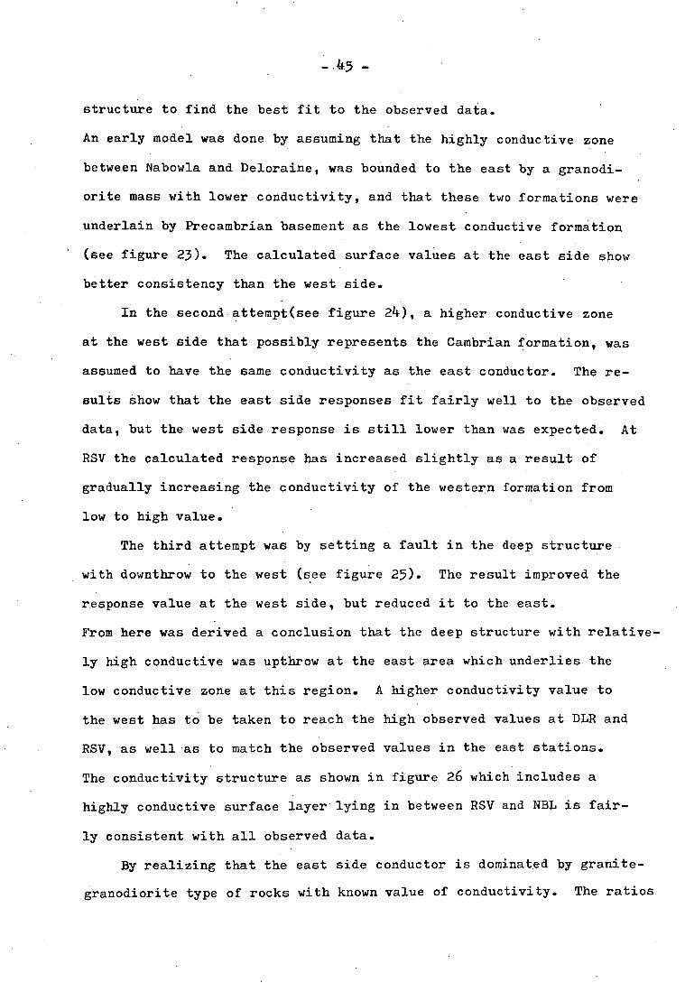
structure to find the best fit to the observed data.

An early model was done by assuming that the highly conductive zone

between Nabowla and Deloraine, was bounded to the east by a granodi-

orite mass with lower conductivity, and that these two formations were

underlain by Precambrian basement as the lowest conductive formation

' (see figure 23). The calculated surface values at the east side show

better consistency than the west side.

In the second attempt(see figure 24), a higher conductive zone

at the west side that possibly represents the Cambrian formation, was

assumed to have the same conductivity as the east conductor. The re-

sults show that the east side responses fit fairly well to the observed

data, but the west side response is still lower than was expected. At

RSV the calculated response has increased slightly as a result of

gradually increasing the conductivity of the western formation from

low to high value.

The third attempt was by setting a fault in the deep structure

with downthrow to the west (see figure 25). The result improved the

response value at the west side, but reduced it to the east.

From here was derived a conclusion that the deep structure with relative-

ly high conductive was upthrow at the east area which underlies the

low conductive zone at this region. A higher conductivity value to

the west has to be taken to reach the high observed values at DLR and

RSV, as well as to match the observed values in the east stations.

The conductivity structure as shown in figure 26 which includes a

highly conductive surface layer lying in between RSV and NBL is fair-

ly consistent with all observed data.

By realizing that the east side conductor is dominated by granite-

granodiorite type of rocks with known value of conductivity. The ratios

^

.2

0

-.2

DLR LLD NBL SCD FRT I I

10 2

S. m -1

.2

0

-.2

-.4

DLR RSV LLD NBL SCD FRT I I

—46—

-1 - 1 10 S.m

-3 10 S.m -3 10 S.m -I

-4 2 x 10 S.m-

Figure 25

.4

a- -10

-20

-30

10-1 S.m -1

5 _10

-20

-1 10-3 S.m

10-2

S.m-1

.4

2X 10 -1 S.

-30

- 2 X 10 4 S.m-

Figure 26

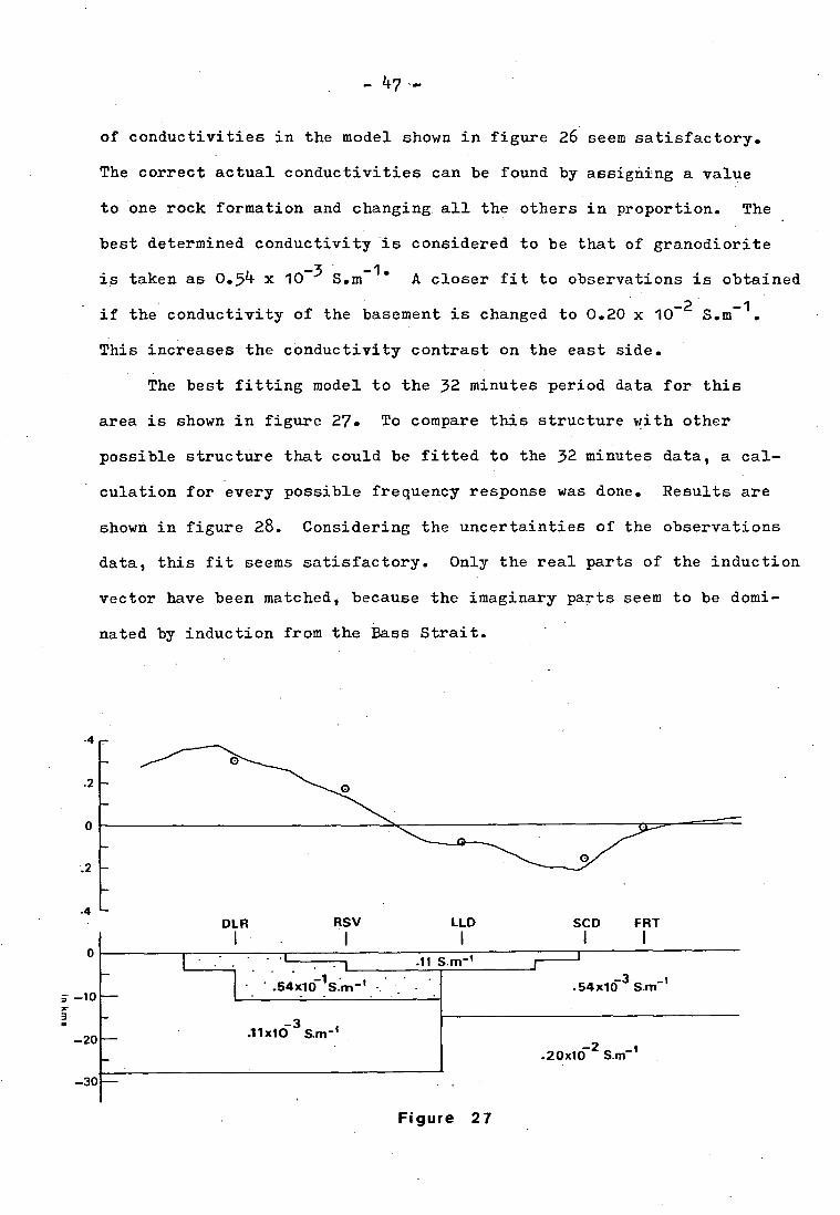
47

of conductivities in the model shown in figure 26 seem satisfactory.

The correct actual conductivities can be found by assigning a value

to one rock formation and changing all the others in proportion. The

best determined conductivity is considered to be that of granodiorite

-3 - is taken as 0.54 x 10 S.m 1. A closer fit to observations is obtained

if the conductivity of the basement is changed to 0.20 x 10 -2 S.m-1 .

This increases the conductivity contrast on the east side.

The best fitting model to the 32 minutes period data for this

area is shown in figure 27. To compare this structure with other

possible structure that could be fitted to the 32 minutes data, a cal-

culation for every possible frequency response was done. Results are

shown in figure 28. Considering the uncertainties of the observations

data, this fit seems satisfactory. Only the real parts of the induction

vector have been matched, because the imaginary parts seem to be domi-

nated by induction from the Bass Strait.

.2

0

.2

.4

DLR RSV LLD SCD FRT

.11 S.m"

' .54x10- • .54x10-3 S.m_ t

-3 .11x10 Sm -1 -20 -2

.20x10 S.m

-30

Figure 27

111-5 INTERPRETATION OF STRUCTURE

The conductivity structure derived from geomagnetic variation

study as shown in figure 28, shows five different conductivities which

have been applied to satisfy the observed magnetic variations as well

as other results such as geology and gravity. Although the determination

'of.the depth, thickness and conductivity of the formations involved are

subject to considerable uncertainty, the few structural features that

are responsible for the anomaly are probably fairly well defined. For

example, the deep structure at a depth of 15 kms in the east side, that

has a conductivity of about 20 times that of the Precambrian basement,

is responsible for complicating the conductive anomaly in the east side,

where the induction -vectors- have relatively small amplitudes and random

in directions, compared to the induction vectors in the west side.

There is no obvious reason why the conductivity of the basement

rock should be higher than either the Precambrian or granodiorite. The

assumption in gravity interpretation is that it is denser than the over-

lying rocks, which suggests a lower porosity. It is unlikely, but

perhaps not impossible, that its increased conductivity is due to higher

temperature.

To the west side the later sedimentations are underlain by Precambrian

crust that has the lowest conductivity value in this region. Since there

is no control of the observed anomaly to the west of Deloraine, the base

of this Precambrian crust in that region is left in question.

The conductivity structure clearly shows that the area in the vi-

cinity between Scottsdale and some kilometers west of Deloraine has the

form of a basin, where sedimentation occured since Cambrian times. Two

highly conductive layers were interpreted in this area. One overlies the

Precambrian basement l -being mainly Cambrian in age, and the other is the

highest conductive layer, probably because of the high quatity of water

filling porous sediments.

T 32

0.0

.2

0.0

—.2

T 16

T 24

0 0.0 T 64

0

—.2

.2

0

0 T 85

0

-

—10km 0

—, o

—20km— — 0

— 30101v—//////1/// /////////////. / //

— 40 kaf Figure 28

Deloraine Rosevale Scottsdale Forester

. 1.. .. . .. . . • . 1::::::::..,.:A..-::.r.;::.::•: ..:-.''.'::;:ii iii Srrit".-f;:::;::.::.1::::-.::::::: I I •/

0 0 0 0 I I

." : .. : .0:5.471.0.. S.m . ' . • . 1 ‘ , 0.54v . . . .

, I ,10 S.m-1 - 1

0 0 -3 -1 0 0 0 \a a 0

o \\

o 0 0 0 0 0 0

o 0 - 0 0 o . 0 0

o 0 0 . o 0 o 0

a o

o.m.do s.m 0 . 0 o 0

-2 0.2(6,10 S.m-1

Mathinna Beds +Tertiary sediments

Devonian granodiorite

Cambrian sediments

Precambrian basement

EM21 upper mantle I

T 51

0.0

—.2

.2

0.0

0

.2

Chapter IV

CONCLUSIONS

Some significant indications have been gained from this geomagnetic

variations study ;

1. Local conductivity anomalies control the variations at periods less

than or equal to 48 minutes, while the deep; sea. effect gives a more

or less uniform direction of the real induction vectors for periods

greater than 64 minutes. The induced current at sea water from the

Bass Strait effects on the imaginary induction vectors at all peri-

ods greater than 16 minutes.

2. The surface high conductive zone with NNW - SSE trend, suspected

from earlier results has been confirmed between east of Deloraine

and west of Scottsdale.

3. There is a deep vertical boundary that separates east formation

from west formation under the Tamar zone. To prove the continuation

of this boundary, more stations to the south are needed.

4: The regional gravity trend in the area indicates a fault at depth

with downthrow side to the west. The derived conductivity structure

is consistent with this assuming that the lower layer ( perhaps up-

per mantle ) is a better conductor.

5. A localized zone of mineralization in between habowla, Scottsdale

and Tayene showsstrong influence on the local conductivity anomaly.

6. Magnetic variation surveys always have small precision in determi-

nation of depth. One of the functions of this survey is to indicate

locations at which magneto-telluric measurements should be done in

the future, and how differences is such measurements may be linked.

The area east of the Tamar River where Z variations are small,

should be suitable for magneto-telluric investigations.

- 50 -

— 51 -

ACKNOWLEDGMENTS

I would like to express my sincere thanks to Dr. W. D. Parkinson

for his encouragement and continuous effort in completing this project,.

and also for his suggestions and discussions during its preparation.

To Dr. R. J. G. Lewis, for his useful help in computing is so much

appreciated.

To all property owners and school masters where I set up the

instruments, for their help in allowing me to use their electric power

and their land for the sites, are gratefully appreciated. Thanks are

also due to Mr. Paul Waller for his useful help in setting up the

instruments and transportation during the field operation.

REFERENCES

Adam, A., 1976. Geoelectric and Geothermal Studies - KAPG, Monograph

Series, Akademiai Kiado Budapest.

Banks, M. R., 1962. Journal of The Geological Society of Australia.,

volume 9, part 2., The Geology of Tasmania.

Banks, R. J., 1969. Geomagnetic variations and the Electrical Conduc-

tivity of The Upper Mantle. Geophys. J. Roy. astr. Soc.,

• vol. 17, 457.

Brewitt, C.R - Taylor and Weaver, J.T.,1976. On the finite difference

solution of two-dimensional induction problems.

• Geophys.J.R.astr.Soc., vol. 47, 375 - 396.

Banks, R.J., 1979. The use of Equivalent Current Systems in the inter-

pretation of Geomagnetic Deep Sounding data.

Geophys.J.R.astr.Soc., vol. 56, 139 - 157.

Chapman, S., 1919. The Solar and Lunar diurnal variations of terrestrial

magnetism.

Phil. Trans. Roy. Soc. A., vol. 218, 1.

Duba, A., Piwinskii, A.J. Santos, M., and Weed, B.C. 1978.

The Electrical conductivity of Sandstone, Limestone and

Granite.

Geophys.J.R.astr.Soc., vol. 53, 583 - 597.

Everett, J.E. 9 and Hyndman R.D., 1967. Geomagnetic variations and the

electrical conductivity structure in south-western

Australia. Phys. Earth Plan. Int. vol. 1, 24 - 34.

Hyndman, R.D., 1963. Unpublished M.Sc Thesis ( Institute of Earth

Sciences : University of British Columbia ).

Honkura, Y., 1971. Geomagnetic variation anomaly on Miyake-jima Island,

Jour. Geomag. Geoelectr., vol. 23, 307 - 333.

- 52 -

- 53 -

Jones, F.W. and Pascoe, L.J., 1971. A general computer program to

determine the perturbation of alternating currents in

a two-dimensional model of region of uniform conductivity

with an embedded inhomogeneity.

Geophys. J. R. astr. Soc., vol. 24, , 3 - 30.

Kanasewich, ., 1973. Time Sequence Analysis in Geophysics., The•

University of Alberta Press, pp. 120.

Klein, D. P., 1971. Geomagnetic time - variation on Hawaii Island

and mantle electrical conductivity., AGU Meeting, 1971.

Klein, D. P., 1972. Geomagnetic time - variations, the Island Effect,

and Electromagnetic Depth Sounding on Oceanic Island.

Thesis Univ. Hawaii.

Lahiri, B. N., and Price, A. T., 1939. Electromagnetic Induction in

non-uniform conductors, and the determination of the con-

ductivity of the Earth from terrestrial magnetic variations.

Phil. Trans. Roy. Soc. A, vol. 237, 64.

Lilley, F. E. M., 1975. Magnetometer array studies : A Review of The

Interpretation of Observed Fields.

Physics of The Earth and Planetary Interiors, vol.10,

pp. 231 - 240.

Lilley, F. E. M., 1976. A magnetometer array Study Across Southern

Victoria and the Bass Strait area, Australia.

Geophys. J. R. astr. Soc., vol. 46, pp. 165 - 184.

Leaman D. E., Symonds, P. A., and Shirley, J. E., 1973. Gravity

Survey of the Tamar Region Northern Tasmania., Geologi-

cal Survey Paper No. 1., Tasmania Department of Mines.

Leaman, D. E., and Symonds, P. A., 1975. Gravity Survey of North-

Eastern Tasmania. Geological Survey Paper No. 2.,

Tasmania Department of Mines.

-54-

Lambert, A., and Caner, B., 1965. Geomagnetic depth-sounding and the

coast effect in Western Canada.

Can. Jour. Earth Sc., vol. 2, 485.

McDonald, K. L., 1957. Penetration of the geomagnetic secular , variation

through a mantle with variable conductivity.

J. Geophys. Research., vol. 62, 117.

Parkinson, W. D., 1959. Directions of Rapid geomagnetic fluctuations.,

Geophys. J. Roy. astr. Soc., vol. 2, 1.

Parkinson, W. D., 1962. : The influence of continents and oceans on geo-

magnetic variations.

Geophys. J. Roy. astr. Soc., vol. 4, 441 - 449.

Pascoe, L. J., and Jones, F. W., 1972. Boundary Conditions and Calcula-

tion of Surface Values for the General Two - Dimensional

Electromagnetic Induction Problem.

Geophys. J. Roy. astr. Soc., vol. 27, 179 - 193.

Parkinson, W. D., and Jones, Fa., 1979. Review of Geophysics and Space

Physics, vol. 17.

Schuster, A., 1908. The diurnal variation of terrestrial magnetism.

Phil. Trans. Roy. Soc. A. 208, 163.

Schmucker, U., 1964. Anomalies of Geomagnetic variations in the South

Western United States.

J. Geomag. Geoelectr., vol. 15, 193 - 221.

Sasai, Y., 1967. Spatial Dependence of Short-period geomagnetic Fluctu-

ations on Oshima Island. Bulletin of The Earthquake Res.

Inst., vol. 45, pp. 137 - 157.

Sasai, Y., 1968. idem ditto., vol. 46, pp. 907 - 926.

Wiese, H., 1962. Geomagnetische Tiefentellurik, Teil II, Geofis. Pura

appl., vol. , 83 - 103.

William, E., 1978. Structural Map of Pre-Carboniferous Rocks of Tasmania,

Department of Mines, Tasmania.

-

Brace, W. F. (1971) Reistivity of saturated crustal rocks to 40 km

based on laboratory measurements. In THE STRUCTURE AND

PHYSICAL PROPERTIES OF THE EARTH'S CRUST, Ed. John G.

Heacock. Amer. Geophys. Un. Monograph 14.

Jones, F. W., and Thomson,D. J., 1974. A Discussion of the Finite

Difference Method in Computer Modelling of Electrical

Conductivity Structures. A Reply to the Discussion by

Williamson, Hewlett and Tammemagi.

Geophys. J. R. astr. Soc. (1974), vol 37, pp. 537 544.

Keller, G. V., and Frischknecht, F. C., 1966. Electrical methods

in geophysical prospecting. Chapter 1, Pergamon Press

Ltd, Oxford.

Williamson, K., Hewlett, C. and Tammemagi, H. Y., 1974. Computer

modelling of electrical conductivity structures,

Geophys. J. R. astr. Soc., vol 37, 533.

Woods, D. V., 1979. Thesis, Australian National University.

PLATE I

EXAMPLES OF THE SUBSTORM EVENTS

up Z

so,,T

Plate I-1

Substorm type variations from Western Junction ( WJC )

and Scottsdale ( SOD )

sent.

L. F -

z.

_ 241 _

- 57

Plate 1-2

Substorm type variations from Deloraine ( DLR ) and

Rosevale ( RSV ).

PPR

so I

PPR 0

117

IR PP 2Y11- 77 0

LLD

se.TI I

58

Plate 1-3

Substorm type variations from Lilydale ( LLD ) and

Pipers River ( PPR ).

!Vrg oozy

WTR

WPR

• •--

wa•••-A E • •

1J

: • : : 1 : 602 . •••

up

so•AT I

TAY ,----

N # 27/3_77

E : —0

5o.T. 1 I

. . , .....

H1 F--

e7 3

r

— 59 —

Plate 1-4

Substorm type variations from West Frankford ( WFR ) and

Tayene ( TAY ).

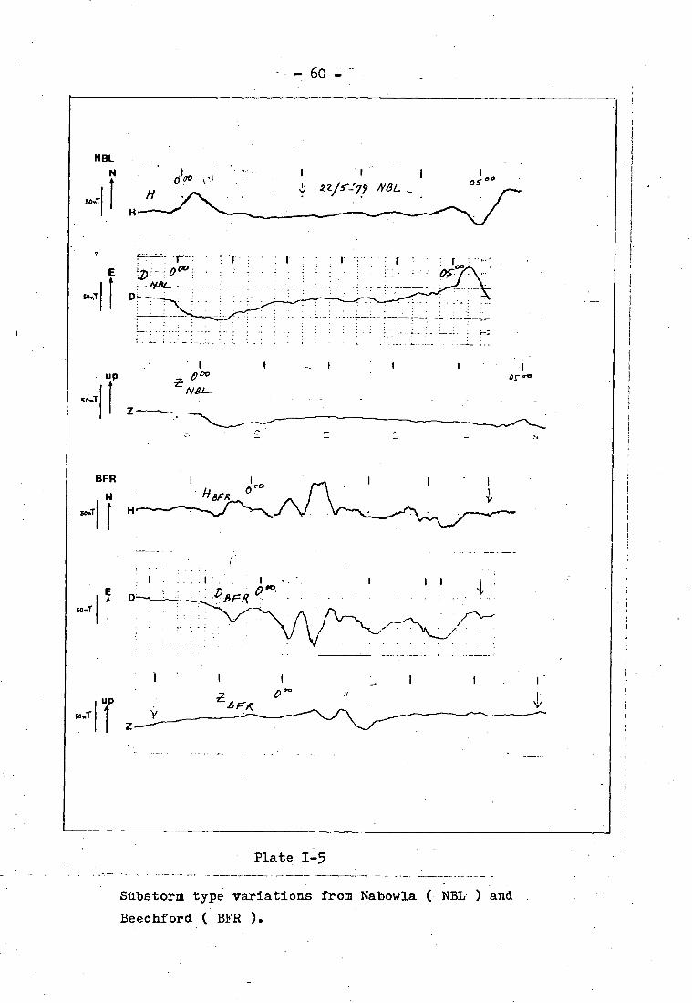
Plate 1-5

Substorm type variations from Nabowla ( NBL ) and

Beechford ( BFR ).

_

so...r u I

r

p

_

' Zefir

ts3

•

, •-•••- v I

I

• •2:`, if I

– 6,3 V I

– 5-.C■ IA I –7'.. A I

—.I,.,.4.4

-I. I

I I

• I

..-

.

":4: CL,

l:.: , 2rit.

0.1 .A

.- .

(2), —

V –

•••••

._• _7 5 rri4k I.

V -..,

•

1 :

......... ... 7' • -_.i o

•.1/.1....:'

.° 4 - : : !

-61.=

Plate 1-6

Substorm type variations from Forester ( FRT ).

PLATE II

PLOTTED TRANSFER FUNCTION VALUES AGAINST PERIODS

Remarks : Ar is the real part of A transfer function (T.F).

Br is the real part of B transfer function (T.F).

A. is the imaginary part of A transfer function (T.F).

B. is the imaginary part of B transfer function (T.F).

•Ar and Br are plotted as a function of periods (T), and

the vertical bars indicate the uncertainty of T.F at a

particular period.

A. and B. are plotted as a function of periods (T), both

in one T.F - T profile, to show-the mirror image chnrac-

teristic between A and B imaginary at almost all stations.

Notice that the uncertainty .values for A and B imaginary

are the same as A and B real, but are not drawn to avoid

a mess.

- 63 -

WJC

A r

T.F

I 4.1

1

-

I 1 I I I I I I I 128 • 64 43 32 26 21 18 16 14 13 m i n .

+.5

0 ------ Ai

B i

-

Plate II-1

- 6 1+ -

DL R T.F

4-5 Ar

^

^

96

48 32 24 19 16 14

12 min.

A i — 0 0-

Plate 11-2

- 65 =

RSV

A r

+•5 B r

I I I 32

24

19

16 3 min•

+ -5 0..

Os A •r‘

•0„

96 I I

48

^

Plate 11-3

-66.

WFR TF

I 1 1 +-5

96 48 32 24 19 16 13 min.

0.... A 1

0

,■••

B •

-•5

Plate II-It

- 67 -

LLD TF

4-5 A r

--5

4-5

I I I I I I I I I I I I I I I 1 I 128 64 43 32 26

21

18

16

14 13 min.

Plate 11-5

- 68

PPR T.F

^

96 48 32 24 19 16 13 min.

-

-

• ----- •

-.5

Plate 11-6

-69

BFR T. F

0

+.5 B r

1-

IIIIIIIIIIIII

+.5 128 64 43 32 26 21 18 16 14 13 min.

".0., . . ,0" ...

, . .. .. '.

-.5

N

Plate 11-7

- 7-0 -

NBL T.F

4..5 A r

••

-.5

+ • 5

0

I

I I I I I I I I I I I I I I I I I 128 64 43 32 26 21 18 16 14 13 min.

I Sp" • - 0, 7 ••-. .•

^

+ • 5

Plate 11.8

+.5 Br

0

- 71 7••

SCD T.F

+ .5 ____ A r ^

-.5

-.5

I I I I I I 128 64 43 32 26 21 18 16 14 13 min.

cy- --c‘, A- .

p----cr - .‘

•

-I- - 5

0

-.5

Plate 11-9

- 72- -

FRT T.F

_ A r

+.5

0 0 0

+.5 128 64 43 32 26 21 18 16 14 13 min.

. ,0

•--

..... •--- .,• •

,

^

-•5

Plate II-10

- 73 —

TAY T.F

+.5

+.5

B r

0

-.5

I 1 I I I 1 1 I I I I I 1 I 96 48 32 24 19 16 13 min.

Plate II-11

PLATE III

COMPUTED SURFACE VALUES FOR PERIODS

85, 64, 51, 32, 24 AND 16 MINUTES FOR

THE BEST FITTED MODEL OF CONDUCTIVITY

STRUCTURE DELORAINE - FORESTER 2 - D

PROFILE.

vaav at Jo aan43na49 aqq. OuTquaseadaa Tapow S4TAT4onpuop

•0 •0

•0 •0 •8

60- •0

-3001 t• ••200/S•

-

▪

3001 1• ▪300/56

•0

3 0

6 9

9

E

0

4I(330 NTYS /149IS

fffifififffEEFFEMEEEEEEfftfifififffiff fEfificiffEEEEEESififEEififififfiEffiESE EiffiffififfEEEfiffEEEfEEEEffEfEfiffffSE iEfifififffiVEEEfiffiiEiiiciffficifififi fifiEciifiEEEffififEEEEEfitifilififfiEci fEiffiiiEfiffEEEEEffEEEEififfEffiEfEffEE EfiiiifififfEffifffiiiiffifffififEffEffi EiffEifiEffEfififESEHEEEfficiffiffiiiff EECEiffiffifEEfEEETEEESEMEEffEfESEEifi iffifififiSiEfiEfffEEEEfiEfifffEffEcifff EffEEfiLEESEEEMESEEEEEEfiffiffiEffifii EffiffiiiifEEEMESEHEEEEfffifESECEME EffififiiiiiffiffiffEEEEEEiciiiiii£Eiffi fffEEifiEffEEEEEEEEEEEEEEEEffliffififEfi EffiEfiiiiffEifitifEEEEEEEFEfiffiffEcifi EEffiffifESEEEfiEfiEfifiiiiifififfEififf EEfiEffiEffEEEfiEffEEEEEEEficiffIffiffEE EffiflEifffEfEfffEfifEEifEEffiffifffEffi EEEEEMIESSEEffiEffEEEEEEEfffiffiiiEfifi EEfiEffifEEEEEfifEfEUEEEEEISEfEHEEEffE EififififfifiEfffiffiifEiEfffififEfffEff EffifififfEEEEEfiffEfifEEfficififiiiiiff

£c222? 22222222222222 91 EfiEffEi.iffEEEfiEfff22222222222222222222 ST

/47/1//22????22227ZWZZ222 ,1 //t1/47////////1/tt/tIIIIIIIIIIIIIIII2222 ET """7"007W07"7"WIIIIIIIIIIIIIIIII2222 21

/IIIIIIIIIIIIIIII2222 II //th/1/////1 /t//,//cSc5;55SSITIIIII2Z22 01 '00007,17.0075 g5555555S5S;555cIIIIITII122 6 '

//55S5SCSS555c5c5CScI1IIII1.1122. /7-5C555C5c5555S5S55c55C5SSITTII22 /

SS5555555555c;c55555555ScITITIZe 9

88F8M:8888R88888883888888888888888888 0000000U00000000000000000000000000000000 .0000000000000000000000000000000000000000 .Z 0000000U00000000000000000000000000000000

6i 9f . /f 9f Sf hf ff 2f If Of 62 92 /2 92 52 1P2 f2 22 12 02 61 9I /I

I. Noilvomimoo 3A113PON00 3H1 •/-

- 75 -

CALCULATED SURFACE VALUES COMPUTED FOR MODEL WITH 85 MINUTES

PERIOD AND STOPPED ON 66 ITERATIONS

AMHY AMHZ HZHY OPHASE DPHA1y OPHAHZ APP RES THEM. T1MAG AME

i 8:33P 4 0.996 5 0.995 6 O. 995 7 0.995 8 Q.994 9 0.994

10 0.993 11 0.993 12 0.993 13 0.992 14 0.992 15 0.992 16 0.991 17 0.991 18 0.991 19 0.991 20 0.991 21 0.990 22 0.990 23 0.990 24 0.990

0.993 0.120 0.121 0.0 14 -2.601 -2.128 .54 5E+14 1.014 0.130 0.177 0.011 -7.79 -1.937 .$2 1E+14 1.069 0.201 0.183 0.009 -2.300 - 1.900 6E+14 ..46 1.092 0.179 0.164 0.007 -2. 281 -1.942 .44 8E+14 1.108 O. 16 9 0.152 0.006 -2.'67 -1.966 .43 5E+14 1.121 O. 16 6 0.143 0.005 -2.759 -1.974 .42 4E+14 1.139 0.166 0.145 0.004 -2.'43 -1.974 .41 1E+14 1.165 O. 14 9 0.128 0.003 -2.214 -2.019 .39 3E+14 1.178 0.128 0.109 0.002 -2.207 -2.096 .38 3E+14 1.185 0.120 0.101 0.002 -2.207 -2.138 .37 9E+14 1.197 0.116 0.097 0.001 -2.197 -2.157 .37 1E+14 1.213 0.103 0.085 0.001 -2.182 -2.24s .361E+14 1.222 0.033 0.068 0 .0 CO -2.176 -2.442 .35 6E+14 1.226 0.068 0.055 0.000 -2.174 -2.759 .35 3E+14 1.227 0.062 0.051 0.000 -2.170 -3.096 .35 2E+14 1.221 O. 06 3 0.052 0.000 -2.177 2.948 .355(414 1.215 0.064 0.053 O.09 -2.181 2.66b .35 9E+14 1.207 0.066 0.054 0.000 -2.185 2.794 .36 3E+14 1.198 0.067 0.056 0.000 - 2.192 2.730 .36 9E+14 1.167 0.065 0.054 0.0 00 -2.199 2.836 .3r 5E+14 1.179 O. 06 3 0.053 0.000 -2. 213 -3.004 .381E+14 1.170 0.065 0.055 0.000 -2.219 -2.866 .38 6E+14 1.162 0.068 0.059 0.000 -2.225 -2.733 .39 1E+14

0.12 0.03

0.16 0.08

0.17 0.07 0.15 0.05 0.15 0.05 0.14 0.04 0.14 0.04 0.13 0.02

0.11 0.01

0.10 0.01 0.10 0.00 0.08 - 0.01 0.07 - 0.02 0.05 - 0.03 0.03 - 0.04 0.02 -0.05 0.02 - 0.05 0.01 - 0.05 0.01 - 0.05 0.02 - 0.05 0.04 - 0.04 0.04 -0.03 0.05 - 0.03

27 0.989 1.149 0.065 0.057 28 O. 969 1.144 0.062 0.054 29 0.963 1.135 0.067 0.059 30 0.988 1.116 0.031 0.072 31 0.988 1.091 0.088 0.081 32 0.967 1.071 0. 09 3 0.087

8:32' 1.045 1.006

0. 10 1 0. 03 3

0.096 0.083

35 0.986 0.996 0. 06 3 0.063 36 0.966 0.994 0.064 0.064 37 0.965 0.995 0.070 0.070 38 0.985 0.996 0.076 0.076 39 0.964 0.999 0.081 0.081 40 0.983 1.002 0.084 0.084

- 0.000 -0.000 - 0.000

-2. e33 -2.235 -2.240

-2.645 3.129 2.724

.39 9E+14

.40 2E+ 14

.40 9E+ 14 0.000 -2.258 2.432 .42 3E+14 0.000 -2. 2 87 2. 336 .44 2E+14 0.001 -2.302 2.283 .45 6E+14 0.001 -2.337 2.219 .431E+14 0.002 -2.401 2. 396 .51 8t+14 0.002 -2.403 2.954 .52 8E+14 0.002 -2.401 - 2.918 .53 0E+14 0.002 -2.399 -2.681 .52 9E+14 0.002 -2.396 -2.546 .52 7E+14 0.001 -2.393 -2.468 .52 3E+14 0.000 -2. 7 91 -2.422 .51 9E+14

8:8(6, =8:8i 0.05 - 0.03 0.03 - 0.04 0.01 -0.06

-0.00 -0.07 -0.01 - 0.08 -0.01 -0.09 -0.01 - 0.10 0.01 -0.08 0.04 - 0.05 0.06 -0.03 0.07 -0.02 0.03 -0.01 0.08 - 0.01 0.08 - 0.00

ia 8:;g9 8:8cf 8:8ti 8:88 =kW

H VALUES20.10. 7. 5. 4. 4. 4. 4. 4. 3. 3. 3. 3. 3. 3. 2. 2. 2. 2. 2. 1. 2. 2. 2. 3. 3. 3. 3. 3. 3. 3. 4. 4. 4.-4. 4. 5. 7.10.20.

K VALUES45.30. 20. 10. 5. 1. 1. 1. 1. 1. 2. 2. 2. 4. 4. 4. 5. 5. 5. 5. 7. 7. 7. 7. 7. 7. 7. 7. 7. 7.10.10.10.10.10.10.10.10.10.10.

SCALE = 100000. FRE() = 0.000196

Plate 111-2

-III 04'e-Ed

ec *5

092000°0

e0I•Oi•0ie0I•01°CI•01'0I'01'0I'i 'S *5 "7 "7 'h '2 °I 'I 'i 'I

'02'0I't "9 "7 "t 17'h '1 'E 'E .2 .2 .2 .2 .2 .2 •2 .2 .2 .4? .*1

= 038J '000001 = 31V3S

°L "2 '1 'I '1''l '1 '1

'I 'S 'CI'02'0£°ShS3nivA

'E 'E 'E *£ "3 '2 *2 *I

eh eh '5 '2 •01•o2s3n1vA H

I0°0- 90•0 1I +3S25° 905'2- 96i'2- 030'0 610'0 9/00 566°0 096'0 Oh 2Vo- /0•0 hI+31ES' 0E9°2- 2017'2- T00°0 £1060 2104'0 166°0 296'0 6£ ivo- 900 hI+39ES° hIR°2- 90,'2- I00°0 290°0 9900 996°0 £96°0 GE hO*0- 50e0 h1+3/f5" 690°5- 90102- 1006o f90°0 2900 L96'0 £96'0 Lf 90°0- E0e0 $71 +3S' 919'2 017'2- I00•0 9900 590°0 196°0 $7P6°0 9E 90'0- 10•C 1I+3fES° IIh°2 I1h°2- I00'0 2900 290'0 166°0 196'0 SE 21'0- f000- 11+361S° 990'2 101°2- 030'0 4;21°0 521°0 500°I S96'0 hE i1°0- 90'0- $71 +3'7'7 996°1 c: '2- 100'0- hhI'D 251'0 2S0e1 596'0 if' 21'0 - 90°0- '71 +35'7'7' 266°1 166'2- ZD0'0- EiTeg 1.110 990°I 996°0 2f 11'0- 50'0- h14392," 110'2 h/262- 2000- .721°0 9E10 III°I 996'0 1E 01'0- SO°0- hI+3E0h° 2c0'2 Ih*Z- E00'0- II1°0 121°0 2hI•1 996'0 OE 90°0- c00- '71 +39ç' 291'2 02c;"2- '700.0- P90e3 £01'0 L9I'1 /P6°0 62 10•0- 100- hi+3/LE° ',1'7'2 EI2°2- h30'0- G90°0 TP0'0 191°1 296°0 92 90,0- 10°0 hi+35LE' 1L9'2 h00'0- /50°0 990'0 691e1 1P6'0 12 S060- 20°0 h1+369E' 999'2 60c;"2- 5000- ESO°0 £90'0 561°1 996'0 92 S0'0- 20'0 h1+399E° £E6'? 01a'2- 500'0- 250°D £90"0 IO2°T 996'0 52 SO°0- 20'0 hI+309E" 909'2 00•2- sOo•o- fS0°0 59060 IT3°I 996'0 h2 S0'0- IO°0 #71+3hSf" 9g9'2 26V2- SIO°0- 550'0 990'0 222'i 696'0 i2 90'0- 00'0 i7I+39hi° £9S'Z 991'2- 5D0'0- 9500 I20'0 SE2°I 696'0 22 /0'0- 10'0- '71+30 'ii:' 01£'2 ILI°2- SO0'0- 690'0 990°0 9h2'I 696'0 12 /0°0- 20°0- h1+3Effe 60E62 E9I°2- SOO°0- 020°0 690'0 092°1 696'0 02 90°0- TO°0- '71 .327ç' E9E'2 SDO°0- 590°0 £90°0 2/2°T 696'0 61 90°0- 00'O- 11+322E° 6/h"2 I51°2- 930'0- 093°0 910°0 252°1 066'0 91 coo- 00'0 11+391E° 209°2 9hI'2- 900°0- SSO°0 IJ0'0 162'1 066°0 IT 50.0- 200 1T+3hIE" 9262 0hi."2- 900'O- 00°0 £90'0 962°1 066'0 91 EO°0- h0e0 '71+3c Ice: 999'?- £'7I'2- 900'O- 050'0 590°0 162'1 066'0 Si 20'0- 90°0 hI43/1E° 6'i'7'2- ShI°2- 900'0- t90°0 E9060 £62°1 166'0 hi 00'0- 60'0 11+322E' 202'2- 0SI"2- 50060- 990'0 01160 £92°T 166°0 ET 10'0 0'1°0 hi+32ES' *760°2- 59I°2- S00°0- '01°0 Me() 592°1 266'0 21 T0'0 II°0 '71+31 '7• 150°2- '700,0- f11e0 Itl'O 9t2e1 266'0 It 200 EI°0 11+39,7E' coo.?- 11172- ED0°0- /21°0 951'0 6E2°1 266'0 OI h0'0 •51•0 hI+3/SE° h£6°1- 591'2- ?00.0- SSI'D 691"G 122°I £66'0-6 90'0 11•0 '71+39/E° £69'i- 912'2- 000°0- 6L1'0 £I2'0 991eI £66'0.9 90'0 P1'0 '71 +36' 999'1- 5E6'2- 100°0 29160 9120 £9I'T h66°C 1 /0°0 91'0 1I+360he 5/96I- hhZ°2- E00'0 /WO 522•0 hhIei '766'0 9 eo•o oz•o '71 +39$7 .SS9'I- 29e°2- S0060 h1?°0 0,2'0 I21°I 566•0 S IT°0 22°0 '71 +3Z5'7• 922°1- 59'6°2- 1000 Sh2'0 9920 6901 566'0 h 2'1•0 02°0 hI+3,cIS° 9/i°2- 1T0'0 17E.2'0 9E2'0 9I0'I 9660 £ 90'0 hI°0 131S5° 966'1- 90h°2- ST0'0 951°0 951'0 9P6'0 966°0 2-

9VWII 1V381 S3NddV ZHVHd0 AHVHd0 3SVHd0 AHZH ZPWV ANWV 3WV

SNONNESII JO HSEINON 013 rIVIOI NO GaddOIS ativ aoplad saIntaw 49 laim 'laurel aHJ HO d aaIndwoo sanqvA OMHOS GaITIflOrIVO

A

AME AMC( AMHZ

2 0.99T 0.950 0.198 3 0.99i 1.018 0.294 4 0.995 1.102 0.327 5 0.994 1.141 0.296 6 0.993 1.170 0.276 7 0.993 1.194 0.265 8 0.992 1.224 0.257 9 0.992 1.2()4 0.226

10 0.991 1.287 0.187 • 1 0.991 1.298 0.163 12 0.990 1.317 0.148 13 0.990 1.339. 0.120 14 0.990 1.350 0.035 15 0.989 1.354 0.063 16 0.989 1.355 0.064 17 0.989 1.346 0.030 18 0.988 1.336 0.091

ig 8:Hg 1:i6 8:1U

1-7Hy CIPHAsE

0.202 0.015 0.289 0.009 0.296 0.004 0.259 0.001 0.23; -0.002 0.22! -0.004 0.211 .-0.006 0.179 -0.006 0.145 -0.010 0.126 -0.011 0.113 -0.012 0.093 -0.013

0.063 -0.013 0.046 -0.014 0.048 -0.014 0.059 -0.013 0.068 -0.013

OpHA1-f7 APPRES

-1.908 .553E+14 -1.805 .512E+14 -1.788 .436E+14 - 1.811 .4D5E+14 -1.829 - .386E+14 -1.840 .370E+14 -1.849 .351E+14 -1.884 .329E+14 -1.945 .311E+14 -1.997 .312E+14 -2.039 .302E+14 -2.150 .292E+14 -2.413 .287E+14 -2.937 .285E+14 2.764 .285E+14 2.193 .283E+14 2.257 .293E+14

:i3=1:1t

OpHAHy

-2. 4 11 -2. 774 -2.270 -2.244 -2.226 -2.215 -2.195 -2.162 -2.153 -2.153 -2.142 -2.126 -2.121 -2.120 -2.116 -2.123 72.128

8:M =8:811 1:1=3.i PAH

- 77 -

CALCULATED SURFACE VALUES COMPUTED FOR THE MODEL WITH 51 MINUTES

PERIOD AND STOPPED ON TOTAL 157 NUMBER OF ITERATIONS

0.987 1.292 0.114 0.088 -0.012 -2.148 2.086 .312E+14 0.967 1.279 0.099 0.0E7 -0.012 -2.164 2.190 .3191+14 0.987 1.263 0.094 0.074 -0.011 -2.1.72 2.232 .321E+14 0.987 1.249 0.089 0.071 -0.011 -2.180 2.z82 .334E+14 0.9or 1.235 0.034 0.063 -0.011 -2.191 2.344 .341E+14 0.985 0.986

1.227 1.218

0.036 0.099

0.071 0.081

-0.010 -0.010

-2.190 -2.192

2.313 2.195

.345E+14

.350E+14 0.985 1.207 0.120 0.099 -0.009 -2.196 2.067 .356E+14 0.985 1.189 0.150 0.126 -0.009 -2.204 1.954 .36/E+14 0.985 1.159 - 0.179 0.154 -0.008 -2.227 1.884 .386E+14 0.964 1.122 0.191 0.170.-0.006 -2.762 1.863 .411E+14 0.984 1.092 0.196 0.189 -0.005 -2.281 1.856 .434E+14 0.963 1.052 0.204 0.194 -0.003 -2.328 1.845 .46/E+14 0.933 0.997 0.170 0.171 -0.002 -2.412 1.910 •519E+14 0.982 0.981 0.113 0.115 -0.001 -2.417 2.115 .536E+14 0.982 0.976 0.082 0.084 0.000 -2. 4 17 2.383 .541E+14 0.961 0.974 0.066 0.068 0.000 -2.415 2.720 - .542E+14 0.980 0.915 0.061 0.063 0.001 -2.413 3.076 .541E+14 0.979 0.978 0.064 0.065 0.001 -2.410 -2.901 .537E+14 0.978 0.982 0.070 0.071 0.000 -2.663 .530E+14

TREAL T1MAC

0.18 0.10 0.24 0.16. 0.26 0.14 0.24 0.11 0.22 0.09 0.21 0.08 0.20 0.07 0.17 0.05 0.14 0.03 0.12 0.02 0.11 0.01 0.09 -0.00 0.06 -0.02 0.03 -0.03 0.01 -0.05

-0.01 -0.06 -0.02 - 0.06

=8:84 =8:8 78 -0.04 -0.08 -0.03 -0.07 -0.02 -0.01 -0.0z -0.07 -0.C1 -0.07 -0.01 -0.07 -0.03 -0.08 -0.04 -0.09 -0.07 - 0.11 -0.09 -0.13 -0.09 - 0.14 -0.10 -0.15 -0.10 -0.17 -0.06 -0.16 -0.02 - 0.11 0.01 -0.08 0.03 - 0.06 0.04 - 0.04 0.06 -0.03 0.01 -0.02

7 1 ?? 23 24 25 26 27 28 29 30 31 32 33 34 35 36 37 38 39 40

vALUES20.10. 7. 5. 1. 2. 2. 2. 3. 3. 3.

K VALUE545.30.20.10. T. 7. 7. 7. r. 7. 7.

4. 4. 4. 4. 4. 3. 3. 3. 3. 3. 3. 2. 2. 2. 2. 2. 3. 3. 3. 3. 4. 4. 4. 4. 4. 5. 7.10.20.

5. 1. 1. 1. 1. 1. 2. 2. 2. 4. 4. 4. 5. 5. 5. 5. 7. 7. 7.10.10.10.10.14.10.10.1D.10.10.

SCALE = 100000. FREQ = 0.000327

Plate III-4

- 78 -

CALCULATED SURFACE VALUES COMPUTED FOR THE MODEL WITH 32 MINUTES

PERIOD AND STOPPED ON 284 TOTAL NUMBER OF ITERATIONS

AME AMAY AMHZ h2HY

2 0.996 0.951 0.309 0.325 3 0.994 1.006 0.428 0.425 4 0.993 1.120 0.464 0.415 5 0.992 1.174 0.422 0.360 6 0.991 1.214 0.393 0. 1 24 f 0.990 1.249 0.374 0.99

0.990 1.291 0.358 0.277 9 0.969 1.344 0.314 0.233

10 0.963 1.376 0.259 0.183 11 0.953 1.391 0.221 0.159 12 0.967 1.416 0.195 0.133 13 0.98r 1.445 0.152 0.105 14 0.966 1.460 0.099 0.C67 15 0.986 1.465 0.060 0.C41 16 0.985 1.465 0.065 0.(44 17 0.985 1.453 0.097 0.C67 18 0.985 1.440 0.122 0.0:15 19 0.964 1.423 0.146 0.103 70 0.984 1.403 0.169 0.121 ?.1 0.964 1.350 0.179 C.130 22 0.983 1.362 0.173 0.127 23 0.983 1.339 0.171 0.123 24 0.983 1.319 0.170 0.129 25 0.983 1.299 0.166 0.127 26 0.982 1.235 0.172 0.134 27 0.982 1.270 0.193 0.152 78 0.961 1.252 0.224 O. J79 ?. 9 0.981 1.226 0.2640.c15 30 0.980 1.135 0.301 0.254 31 0.980 1.134 0.316 0.279 32 0.979 1.094 0.322 0.294 33 0.979 1.040 0.330 0.317 34 0.978 0.969 0.284 0.293 35 0.977 0.947 0.206 0.217 36 0.977 0.938 0.157 0.167 37 0.976 0.935 0.121 0.130 38 0.975 0.934 0.094 0.101 39 0.974 0.936 0.074 0.C79 40 0.972 0.940 0.061 0.C65

OPHAH2 APF) RES. TREAL TIMAC

-1.805 .553E.14 0.27 0.19 -1.756 .492E+14 0.35 0.24 -1.750 .396E+14 0.37 0.19 -1.769 .35 9E+14 0.33 0.15 -1.783 .336E+14 0.30 - 0.13 -1.794 .311E.14 0.28 0.11 -1.803 .296E+14 0.26 0.10

.-1.829 .27 3E+14 0.22 0.07 -1.872 .260E.1.4 0.18 0.04 -1.912 .254E414 g.16 0.01 -1.950 .24 14 .14 0.0e -2.040 .23 5E+14 0.10 0.00 -2.271 .230E+14 0.07 - 0.01 -2.884 .228E.14 0.03 - 0.03 2.553 .226E+14 -0.00 -0.04

- 2.111 .231E+14 -0.03 - 0.06 1.973 .236E.14 -0.05 - 0.07 1.887 .241E.14 -0.07 -0.08 1.831 1.814

.Z48E+14

.25 6E+14 -0.08 -0.09

-009 - 0.09

1.829 .26 3E+14 -0.09 - 0.09 1.834 .271E+14 -0.09 -0.09

.2 9 4E+14 -0.09 - 0.10

.301E+14 - 0.10 - 0.11

.309E14 -0.13 -0.13

.322E.14 -0.16 - 0.15

.345E.14 -0.19 -0.17

.376E+14 -0.20 -0.20

.404E+14 -0.20 - 0.21

.447E.14 -0.21 -0.24

.513E+14 -0.16 -0.25

.537E.14 -0.10 -0.19

.54b'14 -0.06 -0.15

.549E+14 -0.03 -0.13

.549E+14 -0.01 - 0.10

.54 6E+14 0.01 -0.08 .

.539E+14 0.03 0.06

(PHASE 013 14AHY

0.0 15 -2.414 0.0 C4 -2.762

- 0.006 -2.739 - 0.012 -2.209 - 0.017 -2.163 -0.021 -2.176 - 0.025 -2.154 - 0.029 -2.121 - 0.032 -2.112 - 0.034 -2.112 - 0.036 - e. 701 - 0.037 -2.086 - 0.038 -2.082 - 0.039 -2.n80 - 0.039 -2.P77 - 0.038 -2.084 - 0.038 -2. 083 - 0.037 -2.n94 - 0.036 -2.101 - 0.035 -2.109 - 0.035 -2.125 -0.034 -2.133

-0.031 2.153 1.837 -0.029 -2.157 1.802 -0.027 -2.161 1.762 -0.025 -2.170 1.725 -0.023 -2.196 1.700 -0.020 -2.236 1.694 -0.017 -2.259 1.694 - 0414 -2.714 1.694 -0.010 -2.419 1.725 -0.007 -2.427 1.806 -0.005 -2.428 1.901 -0.004 -2.427 2.024 -0.002 -2.426 2.193 -0.001 -2. 4 23 2.438

0.000 -2.418 2.810

1:811 11:Iti :i83E:lt :813 =8:18

73: 1: 1: 1: 1: t: 4: !: P.10: e 2. 2. 2g.

K VALUES45.30.20.10. 5. 1. 1. 1. 1. 1. 2. 2. 2. 4. 4. 4. 5. 5 . 5. 5. 7. 7. 7. 7. 7. T. 7. 7. 7. 7.10.10.10.10.10.10•10.10.10.10.

Plate 111-5

/69000°0

'0T*OT'OT*OT*0T*OT'OT'OI°0160I'/

"5 'S 'S *1 *h 't '2 '2 '2 'I 'I 'T 'T

02'01'2 •5 6h 't *t *h 'h °E *£ '2 '2 '2 *2 62 'E 'E 'E 'E 'E *h

= 0383 *000001 = 31V0S

*/ */ 6/ */ '/ '2 "1 '/ 'A 'I 'S e01•02e0ies.7s3n1vA

'E 'E 'f °E 'i '2 '2 "2 *I 'I 'S '/ 60T•02S2n1VA

600- 00•0- hT+3ihS• 6E2'2 h2,2"2- 0000 2600 £90°0 S06'0 99660 Ot 2.1"0- £0'0- hT+3A4S• YEO*2 6212- i00'0- 2?1°3 011'0 ICC° 0/60 6i hT60- 9060- hT+32SS 0161 2E1'2- 9000- SSI°0 Ohl'O 1060 116°0 9i /T*0- 60°0- s7T+30sS• EZ9•I Z£v*Z- 90000- £610 I/T*0 206'0 216°0 /i IZ*0- 210- ht+3ShS' 9S1'I 2E7'2- TIO*0- 6E2'0 /12*0 106'0 1/60 9£ 52*0- 910- 71+3EiS6 00/°1 0E112- h10'0- 962°0 h22*0 9160 i16'0 SE Ii'0- £2'0- 4I43/OS° 91961 02,1'2- 6t00- t9E°0 E9E60 5,6°0 h/6'0 tE 620- 920- hI+392h* 9291 fOi'2- 0'i0 II,*0 920°1 S160 if SZ60- 92•0- /1+309E" E29*1 fh2°2- 0O•0- 2/E°0 S0h°0 060°T S/6'0 2£ 2Z0- 61°0-

ia•o- 540-

t7I+647• hi+JSTE°

IZ91 Ee9°1

hiO'Q- ILL'e- 9E0'0-

CSE*0 81i60

96f*0 18E'0

9E1'1 161*T

SI6'0 916°0 1E Oi

910- 220- 11+3162' 1E9'1 1S1.2- 2h0'0- 1/20 /fE'0 9t261 /16'0 62 '1'0- gi•O- h1+3912• 65961 Sh1*2- coo- 122'0 162°0 112°1 116•0 92 'ID- S1'0- '71+3692' 299*1 9E1'2- 9h0'0- 961•0 15.2•0 00i°1 9/6'0 a II*0- EI*0- /1+3192' EOL'I OSO*0- E1I*0 922'0 STE'T 9160 92 II°0- ET'O- 41+3552' VIVI 5E1'2- ESO*0- 191'0 612'0 9ff'T 616'0 S2 010- £1*0- 11+39h2' 101*1 /21'2- tSO*0- 291.'0 122'0 6SE'T 6160 /2 010- 210- /1+32E2' 902'1 SIi'2- 9500- 9SI60 612'0 tEE•T 0916°0 £2 01°0- 210- h1+3622" 90/*1 101'2- /S0'0- tS1*0 91260 017*T 096'0 ?2 6060- 2'1'0- 41+3222* SOL*1 26u*2- 9SO*0- ISI"O 9120 Ift*T 096'0 12 9060- I160- /1+3/12' 1211 19u*2- 6500- /iI*0 0020 9Sh'1 096'0 02 /0'0- 60'0- h1+39026 69161 Itu°2- t900- 4;1160 0/1'0 28.7'1 196'0 61 900- 10'0- ,7I+3i0Z° 919°1 2/u.2- ?900- 1600 LET°0 105'1 1960 91 G00- h3*0- 41+3661* 196'1 99062- 290•o- 690'0 '0'1'0 /1S6T 1P60 AT ,70•0- 10'0- 11+3S6I* ElLh'2 19u"2- £90'0- Oh060 1900 OES'T 29600 91 E0'0- E0'0 h1+35,61* •75/02- S9u*Z- £9O0- 6£0•0 090°0 OfSoi 296'0 ST 100- /00 P/1+314516 9/1*2- 99u'2- 2900- h100 £l1'0 IZS".1 f96'0 IT 100 21°0 11+3202* 266•1- 0/u02- t900- SIT'0 911'0 9CS61 E96'0. ET £00 1060

SI*0 91'0

/I+31I2' h1+3022*

0261- 6991-

h9U*2- 6500- '60'2- 9;0'0-

/ST*0 1E2'0 479Z•0 vh/ot

,96'0 S96'0

'?1 tt

SO*0 T2'0 '71+3922' 959'1- 6u '2- iS0°0- 1120 OTE°0 92/*1 596'0 01 /0'0 92'0 h1436£2* 1291- 2012- 6h0"0- 692110 11E°0 69E61 9960 6 II'0 210

OE'0 fi•0

11+3E92' hi+Jtsee

009'1- 16161-

SWZ- EhO'0- Sst6z- /0.0-

22E°0 OSE*0

/21°0 1ht°0

92161 912'1

1960 9 996•0,/

hI°0 SE°0 h1+3h0f* 09/*1- /91'2- TEO*0- 19E*0 1P7•0 Sf2°1 6P609 /T*0 6E°0 41+362i' /92'T- 691'2- h20'0- /2'7°0 /05'0 991'1 0660 S 22'0 hl'O h1+369f' P14°I- 02Z°2- ST0'0- SWO 955'0 £21'T 166'0 h 0£*0 Esr'0 h1+311h° 61/*1- SS i'2- 2000- £26°0 /15°0 0660 f660 SZ'O h£'0 IT+32Sq* 29/9- S1h*2- hi0.0 91h'O 99E*0 •260 S66*0 2

911wI1 1v3B1 s3eddv zHvHdo ANYHdE 3SVI4c10- ANZH ZWWV ANWV 3WV

smonvHaII JO Hagwilm VLOL L$3 NO aaddOIS UNV UOINgd SHInNIN 42 HLIM amow SU, ao. aaIndwoo sanrivA aovans aaIvringivo.

-6L-

-8o-

CALCULATED SURFACE VALUES COMPUTED FOR THE MODEL WITH 16 MINUTES

PERIOD AND STOPPED ON TOTAL 500 NUMBER OF ITERATIONS

AME AMHY AMHZ HZHY ()PHASE DPHAHy OPHAHz APPRES TREAL TIMAG

(8:3N 00:$ 75(4 8:tit 00:2N 8:3gt (1:nS 2:t 006

6'0.9o3 1.261 0.577 0.457

4:81i 1 :1:c2,2 : 77 791 -I.ec5

7 0.962 1.312 0.547 0.417 -0.069 -2.137 -1.816 8 0.980 1..373 0.521 0.379 -0.079 -2.118 -1.826 9 0.979 1.449 0.457 0.315 -0.0E8 -2.088 -1.844

10 0.978 1.495 0.380 0.254 -0.095 -2.082 - 1.871 11 0.977 1.518 0.323 0.213 -0.099 -2.083 -1.897 12 0.977 1.554 0.281 0.181 -0.1C3 -2.075 -1.921 130.976 1.593 0.216 0.135 -0.107 -2.063 - 1.973 14 0.975 1.614 0.134 0.083 -0.1 09 -2.060 -2.105

8:3R 1 -15i 00:?Ag =8:118 =i:fr'N 17 0.974 1.606 0.113 0.070 -0.109 -2.062 1.792 18 0.973 1.588 0.157 0.099 0.105 -2.n65 1.675 19 0.973 1.564 0.200 0.123 -0.1C7 -2.'70 1.613 20 0.973 1.536 0.241 0.157 -0.105 -2.076 1.576 21 0.972 1.503 0.264 0.176 -0.102 -2. 0 62 1.563 22 0.972 1.476 0.274 0.186 -0.1 G1 -2.096 1.5E3 23 0.972 1.446 0.279 0.193 -0.099 -2.102 1.563 24 0.972 1.416 0.236 0.202 -0.096 - 2.110 1.563 25 0.971 1.387 0.237 0.207 -0.094 -2.120 1.565 260.971 1.365 0.300 0.220 -0.090 -2.119 1.562

g 8:3R 1:111 =8:8gi -2.122 1.552

29 0.969 1.275 0.433 0.340 -0.075 -2.133 1.531 30 0.969 1.215 0.436 0.401 -0.069 -2.158 1.525 31 0.968 1.142 0.508 0.444 -0.062 -2.700 1.527 32 0.968 1.033 0.517 0.477 - 0.055 -2. 724 1.534 33 0.967 1.005 0.528 0.526 -0.046 -2.?88 1.5 4 0

it 8:M 00:g6 g:Va, E:7418 =8:8A -2.623 1.557

36 0.965 0.858 0.300 0.351 -0.023 -2.438 1.621 37 0.965 0.851 0.250 0.294 -0.018 -2.440 1.653 38 0.964 0.848 0.208 0.245 -0.013 -2.440 1.703 39 0.962 0.847 0.171 0.202 -0.007 - 2.438 1.762 40 0.961 0.849 0.134 0.153 0.000 -2.435 1.854

.552E+14 0.45

.455E+14 0.56 8:ig 8:73 86.B

.260E+14 0.43 0.15 • 24 0E+14 • 0.40 0.13 . 213E+14 0.36 0.11 .195E+14 0.31 0.08 .183E+14 0.25 0.05 .178E+14 0.21 0.04 .169E+14 0.18 0.03 • 161E+14 0.13 0.01 .156E+14 0.08 - 0.00

:1M:lt -8:81 =8:8i • 15 1E+14 - 0.05 -0.05 .161E+14 - 0.08 - 0.06 .166E+14 - 0.11 -0.07 . 172E14 - 0.14 -0.08 .179E1'. -0.15 - 0.08 .185E+14 -0.16 - 0.09 . 193E+14 - 0.17 -0.10 . 202E+14 -0.17 -0.10 .210E+14 - 0.18 - 0.11 • 21 7E+14 -0.19 - 0.11

:M:1,4, =8:g .247E+14 -0.29 -0.17 .272E+14 -0.34 - 0.21 .303E+14 -0.37 "0.25 .342E+14 -0.39 -0.28 .397E+14 - 0.41 - 0.33

6.tgi:1 44 =8:P =8:i; .)42E14 - 0.21 -0.28 .550E+14 -0.17 -0.24 .553E+14 -0.13 -0.21 . 553E+14 -0.10 - 0.18 .543E+14 - 0.06 -0.14

H VALUES20.10. 7. 5. 4. 4. 4. 4. 4. 3. 3. 3. 3. 3. 3. 2.2. 2. 2. 2. 1. 2. 2. 2. 3. 3. 3. 3. 3. 3. 3. 4. 4. 4. 4. 4. 5. 7.10.20.

K VALUES45.30.20.10. 5. 1. 1. 1, 1. 1. 2. 2. 2. 4. 4. 4. 5. 5. 5. 5. 7. 7. 7. 7. 7. 7. 7. 7. 7. 7.10.10.10.10.10.10.10.10.10.10.

SCALE = 100000. FRE0 = 0.001042

Plate III-7

APPENDIX I

LISTS OF CALCULATED TRANSFER FUNCTION

OF STATIONS :

1. Western Junction

2. Scottsdale

3. Deloraine

4. Rosevale

5. Lilydale

6. Pipers River

7. West Frankford

8. Tayene

9. Nabowla

10. Forester

11. Beechford

Appendix_I

CALCULATED TRANSFER FUNCTIONS

Station name : Western Junction

Events used : 14

Sampling interval : 2.0 minutes

Recording period : 9/2-1978 until 13/3-1978

Period : 128.0 minutes Real Imaginary Uncertainty

A -0.31 +0.30 + 0.18 - B +0.21 +0.08 + 0.18

Period : 64.0 minutes

A -0.12 +0.33 + 0.17

B +0.24 -0.02 + 0.20

Period : 42.7 minutes

A +0.03 +0.26 + 0.21

B +0.16 -0 .07 + 0.13

Period : 32.0 minutes

A +0.04 +0. 27 + 0.19

B +0.12 -o.o6 + 0.13

Period : 25.6 minutes

A +0.11 +0 . 27 0.27

B +0.07 -o.o8 + 0.21

Period : 21.3 minutes

A +0.10 +0.08 + 0.18

B +0.06 +0.01 + 0.12

Period : 18.3 minutes

A +0.09 +0.09 + 0.21

B +0.09 -0.02 + 0.15

Period : 16.0 minutes

+0.13 +0.10 + 0.19 -

B +0.09 -0.01 + 0.18

Period : 14.2 minutes

A +0.04 +0.06 + 0.16

+0.12 +0.01 + 0.14 _

Period : 12.8 minutes

A +0.14 +0.03 4- 0.17

B -0.01 +0.06 + 0.17

- 82-

-83- •_

Station name : Scottsdale

Events used : 11

Sampling interval : 2.0 minutes

Recording period : 15/3-1978 until 13/5-1978

Period : 128.0 minutes Real Imaginary. Uncertainty

A -0.38 +0.22 + 0.31

B +0.17 -0.67 + 0.24

Period : 85.3 minutes

A *-0.26 +0.26 + 0.27 B +0.15 +0.10 + 0:35_

Period : 64.0 minutes

A -0.25 +0.26 + 0.20

B +0.15 -o.o6 + 0:16

Period 51.2 minutes

A -0.33 +0.08 + 0.25

B +0.14 -0.11 + 0.17

Period 42.7 minutes

A -0.27 +0.16 + 0.28

B +0.04 -0.15 + 0:21

Period : 36.6 minutes

A -0.04 +0.17 + 0:22

B -0.04 -0.20 + 0.17 -

Period 32.0 minutes

-0.16 +0.22 + 0.19

B +0.07 -0.25 + 0.19

Period : 28.4 minutes

A -0.18 +0.08 + 0.16 - B -0.07 -0.20 + 0.20

Period : 26.6 minutes

A -0.14 +0.10 + 0.15 - B +0.10 +0.01 + 0.28

Period : 23.4 minutes

A -0.19 +0.10 + 0.17 -

B -0.13 -0.17 + 0.11

Period : 21.3 minutes

A +0.03 +0.02 + 0 . 16 -

B -0.11 -0.22 + 0.23

- 84 -

Period : 19.7 minutes Real Imaginary Uncertainty

A -0.14 +0.09 + 0.14

B -0.05 -0.09 + 0.16

Period : 18.3 minutes

A -0.15 +0.04 + 0.24

B -0.19 -0.05 + 0.34

Period : 17.1 minutes

A -0.21 +0.01 + 0.18 - B -0.03 +0.05 + 0.15 -

Period : 16.0 minutes

A -0.15 +0.03 + 0.16

B -0.03 -0.06 + 0.16

Period : 15.1 minutes

A -0.04 -0.03 + 0.12 - B +0.04 -0.13 + 0.11 -

Period : 14.2 minutes

A -0.18 -0.02 + 0.29

B -0.20 -0.06 + 0.42 - Period : 13.5 minutes

A -0.04 -0.03 + 0.16

B +0.04 +0.05 + 0.19

Period : 12.8 minutes

A +0.06 -0.03 + 0.16

B -0.15 -0.03 + 0.16

-85-

Station name : Deloraine

Events used

:9

Sampling interval

: 6.0 minutes

Recording period

: 10/6-1978 until 16/9-1978

Period : 96.0 minutes Real Imaginary Uncertainty

A -0.21 +0.39 + 0.26

B +0.17 -0.05 + 0.20

Period : 48.0 minutes

A +0.16 +0.38 + 0.43

B +0.15 +0.09 + 0.30

Period : 32.0 minutes

A +0.32 +0.44 + 0.26

B +0.12 -0.08 + 0.20

Period : 24.0 minutes

A +0.15 +0.34 - 0.31

B +0.17 +0.06 + 0.32

Period : 19.2 minutes

A +0.28 +0.28 + 0.32

B +0.13 +0.06 + 0.31

Period : 16.0 minutes

A +0.48 +0.22 + 0.49

B +0.10 -0.04 + 0.37

Period : 13.7 minutes

A +0.15 +0.04 + 0.23

B +0.25 +0.04 + 0.16

Period : 12.0 minutes

A +0.40 +0.04 + 0.25

B +0.38 +0.00 + 0.31

- 86 -

Station name : Rosevale

Events used

: 13

Sampling interval

: 6.0 minutes

Recording period

: 16/9-1978 until 20/10-1978

Period : 96.0 minutes Real Imaginary Uncertainty

A -0.12 +0.49 + 0.28 - B +0.23 -0.12 + 0.48

, Period : 64.0 minutes

A -0.04 +0. 38 + 0.23 - B +0.13 0.00 + 0.23

Period 48.0 minutes

A +0.09 +0.23 + 0.21

B +0.03 +0.04 + 0.12

Period : 38.4 minutes

A +0.04 +0 . 10 ± 0.15 B -0.07 +0.12 + 0.16

Period : 32.0 minutes

A +0.17 +0.18 + 0.26 B +0.06 -0.02 + 0.34

Period : 27.4 minutes

A +0.12 +0.15 + 0.17

B +0.07 +0.01 + 0.17

Period : 24.0 minutes

A +0.20 +0.13 + 0.25

B +0.06 +0.02 + 0.25 - Period : 21.3 minutes

A +0.04 +0.06 + 0.15 - B -0.01 +0.17 + 0. 15

Period : 19.2 minutes

A +0.12 +0.03 + 0.13 - B -0.02 +0.11 + 0.12

Period : 17.5 minutes

A +0.07 -0.03 + 0.12 - B -0.01 +0.22 ± 0.13

- 87 -

Period

Period

Period

Period

:

:

:

16.0 minutes

14.8 minutes

13.7 minutes

12.8 minutes

A

B

A

B

A

B

A

B

Real

+0.15

+0.06

+0.20

0.00

+0.27

-0.03

+0.12

-0.15

Imaginary

-0.03

+0.08

+0.06

+0.14

-0.02

-0.05

+0.02

+0.09

Uncertainty

+ 0.12 - + 0.20 -

+ 0.15 - + 0;25

+ 0.19 - + 0012

+ 0.15 - + 0.19

- 88 -

Station name : Lilydale

Events used : 9

Sampling interval : 2.0 minutes

Recording period : 20/10-1978 until 8/12-1978

Period : 128.0 minutes Real Imaginary Uncertainty

A -0.34 +0.17 + 0.33

B +0.13 -0.09 + 0.14 - _ Period : 85.3 minutes

A -0.17 +0. 15 + 0.21 - B +0.07 -0.14 + 0.19

Period : 64.0 minutes

A -0.19 +0. 15 + 0.33 B +0.02 -0.10 + 0.25

Period : 51.2 minutes

A -0.15 +0.19 + 0.14

B +0.05 -0. 13 + 0.13

Period : 42.7 minutes

A -0.05 +0.18 + 0.16

B -0.03 -0.18 + 0.25

Period : 36.6 minutes

A -0.07 +0.21 + 0.16

B -0.01 -0.19 -

+ 0.14

Period : 32.0 minutes

A -0.03 +0. 19 + 0.21

B -0.08 -0.15 + 0.17

Period : 28.4 minutes

A +0.02 +0.18 + 0.19

B -0.08 -0.16 + 0.19

Period : 25.6 minutes

A -0.08 +0.11 + 0.16

B -0.04 -0.12 + 0.13

Period : 23.3 minutes

A -0.05 +0. 17 + 0.18

B -0.05 -0.16 + 0.14

- 89 -

Period : 21.3 minutes Real Imaginary Uncertainty

A +0.02 +0.10 + 0.17 - B -0.11 -0.12 + 0.20

Period : 19.7 minutes

A -0.02 +0.09 + 0.10

B -0.05 -0.12 + 0.15

Period : 18.3 minutes

A 0.00 +0.04 + 0.15

B -0.10 -0.09 + 0.17

Period 17.1 minutes

A -0.04 +0.11 + 0.16 - B -0.07 -0.09 + 0.11

Period 16.0 minutes

A +0.02 +0.11 + 0.12 - B -0.02 -0.06 + 0.11

Period : 15.1 minutes

A 0.00 +0.04 + 0.08

B -0.08 -0.07 + 0.10

Period : 14.2 minutes

A -0.03 +0.03 + 0.16

B -0.12 -0.03 + 0.13

Period : 13.7 minutes

A 0.00 +0.02 + 0.03

B -0.07 -0.02 + 0.08

Period : 12.8 minutes

A -0.03 +0.09 + 0.02

B +0.03 -0.10 + 0.03

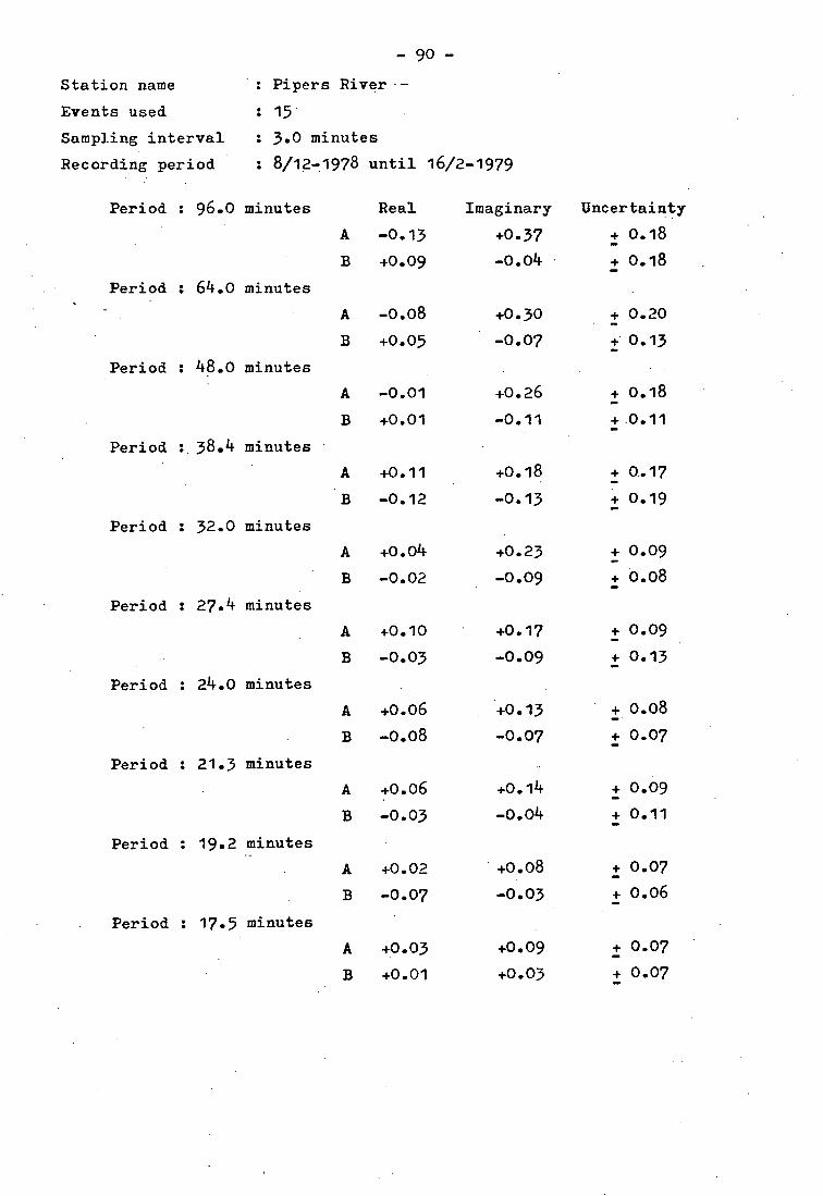
Station name

Events used

Sampling interval

Recording period

- 90 -

: Pipers River.-

:15

: 3.0 minutes

: 8/12-1978 until 16/2-1979

Period : 96.0 minutes Real Imaginary Uncertainty

-0.13 +0.37 + 0.18

B +0.09 -0.04 . + o.18

Period : 64.0 minutes

A -0.08 +0.30 + 0.20

B +0.05 -0.07 + 0.13

Period : 48.0 minutes

A -0.01 +0.26 + 0.18

B +0.01 -0.11 + .0.11

Period : 38.4 minutes

A +0.11 +0.18 + 0.17

-0.12 -0.13 + 0.19

Period : 32.0 minutes

A +0.04 +0.23 + 0.09

B -0.02 -0.09 + 0.08

Period : 27.4 minutes

A +0.10 +0.17 + 0.09 -

B -0.03 -0.09 + 0.13

Period : 24.0 minutes

A +0.06 +0.13 + 0.08

B -0.08 -0.07 + 0.07

Period : 21.3 minutes

A +0.06 + 0.09

B -0.03 -0.04 + 0.11

Period : 19.2 minutes

A +0.02 +0.08 + 0.07

B -0.07 -0.03 + 0.06

Period : 17.5 minutes

A +0.03 +0.09 + 0.07

+0.01 +0.03 + 0.07

91 -

Period : 16.0 minutes Real Imaginary Uncertainty,

A +0.13 +0.06 + 0.11 - B -0.16 -0.11 + 0.15

Period 14.8 minutes

A +0.03 +0.04 + 0.07

-0.09 -0.01 + 0.09

Period : 13.7 minutes

A +0.02 +0.05 + 0.07 -

B -0.04 -0.03 + 0.06

Period : 12.8 minutes

A +0.09 +0.04 + 0.09

B -0.11 -0.01 + 0.10

- 92 -

Station name : West Frankford

Events used

: 15

Sampling interval

: 3.0 minutes

Recording period

: 16/2-1979 until 20/3-1979

Period : 96.0 minutes Real Imaginary Uncertainty

A -0.13 +0.34 + 0.19 - B +0.09 -0.06 + 0.15 _

Period : 64.0 minutes

+0.03 +0.26 + 0.16 - B +0.15 -0.01 + 0.13

Period : 48.o minutes

A +0.06 +0.26 + 0.13 - B +0.12 -0.05 + 0.07

Period : 38.4 minutes

A +0.10 +0.23 + 0.15

B +0.06 -0.04 + 0.16 _ Period : 32.0 minutes

+0.16 +0.19 4. 0.11 - B +0.02 -0.03 + 0.12

Period : 27.4 minutes

A +0.12 +0.17 + 0.15 - B +0.05 -0.08 + 0.15

Period : 24.0 minutes

A +0.22 +0.14 + 0.14

B +0.07 -0.05 + 0.17

Period : 21.3 minutes

A +0.23 +0.16 + 0.14 - +0.05 -0.04 + 0.15

Period : 19.2 minutes

A +0.25 +0.07 + 0.30 - +0.03 -0.03 + 0.11

Period : 17.5 minutes

A +0.19 +0.06 + 0.17

+0.04 -0.09 + 0.15

- 93 -

Period : 16.0 minutes Real Imaginary Uncertainty

A +0.19 +0.01 + 0.11

+0.01 -0.02 + 0.15

Period : 14.8 minutes

A +0.21 +0. 05 - 0.15

B 0.00 -0.01 + 0.15

Period : 13.7 minutes

A +0.18 +0.03 + 0.13

+0.02 +0.01 + 0.12

Period : 12.8 minutes

A +0.19 +0.03 + 0.13 - B -0.03 0.00 + 0.15

- 94 -

Station name

Tayene

Events used

: 15

Sampling interval

: 3.0 minutes

Recording period : 20/3-1979 until 12/4-1979

Period : 96.0 minutes Real Imaginary Uncertainty

A -0.30 +0.07 + 0.23 - B +0.11 -0.21 + 0.35

_Period : 64.0 minutes

A -0.30 +0.14 + 0.19

B -0.01 -0.12 + 0.16

Period : 48.0 minutes

A -0.07 -0.05 + 0.19

B -0.06 -0.28 + 0.28

Period : 38.4 minutes

A -0.16 +0.11 + 0. 33 B -0.15 -0.31 + 0.26

Period : 32.0 minutes

A +0.12 +0.04 + 0.22

B -0.10 -0.1 7 + 0.20

Period : 27.4 minutes

A -0.09 -0.12 + 0.33 B -0.29 -0.11 + 0.32

Period : 24.0 minutes

A +0.12 +0.13 + 0.29

B -0.14 -0.29 + 0.30

Period : 21.3 minutes

A +0.05 -0.02 + 0.21

B -0.18 -0.05 + 0.24

Period : 19.2 minutes

A +0.20 -0.04 + 0.22

B -0.04 0.00 + 0.18

Period : 17.5 minutes

A +0.22 +0.07 + 0.23 -

B -0.04 -0.18 + 0.21

- 95 -

Period : 16.0 minutes Real Imaginary Uncertainty

A +0.11 0.00 + 0.19

B -0.11 -o.o8 + 0.23

Period : 14.8 minutes

A 0.00 +0.11 + 0.27

B +0.16 -0.09 + 0.29

Period : 13.7 minutes

A +0.04 +0.02 + o.4o

B +0.31 +0.02 4. 0.32

Period : 12.8 minutes

A +0.03 -0.02 + 0.21

B +0.23 +0.06 + 0.30

- 96 -

Station name : Nabowla

Events used

: 12

Sampling interval

: 2.0 minutes

Recording period

: 12/4-1979 until 3/7-1979

Period : 128.0 minutes Real Imaginary Uncertainty

A -0.37 +0.25 + 0.34 - B +0.14 -0.10 + 0.26

Period : 85.3 minutes

A -0.30 +0.23 + 0.37

B +0.01 -0.23 + 0.26

Period : 64.0 minutes

-0.36 +0.25 + 0.31

B -0.03 -0.23 4- 0.24

' Period : 51.2 minutes

-0.31 +0.31 + 0.33

B +0.03 -0.24 + 0.41 -

Period : 42.7 minutes

A -0.37 +0.17 + 0.35 -

B +0.06 -0.13 + 0.25

Period : 36.6 minutes

A -0.40 +0.22 + 0.37

B -0.05 -0.12 + 0.28

Period : 32.0 minutes

A -0.27 +0.31 + 0.35

B +0.05 -0.25 + 0.29

Period : 28.4 minutes

A -0.37 -0.02 + 0.33 -

B -0.18 -0.16 + 0.22

Period : 25.6 minutes

A -0.20 +0.23 + 0.28

B -0.12 -0.14 + 0.20

Period : 23.3 minutes

A -0.52 +0.15 +o.41 -

B -0.06 -0.17 + 0.31

- 97 -

Period : 21.3 minutes . Real Imaginary Uncertainty

A -0.20 +0.23 + 0.21

-0.11 -0.23 + 0.24

Period : 19.7 minutes

-0.32 +0.14 + 0.29

B -0.05 -0.28 + 0.25

Period : 18.3 minutes

A -0.29 +0.27 + 0.36

B -0.01 -0.14 + 0.19

Period : 17.1 minutes

A -0.54 -0.08 + 0.42

B -0.15 -0.14 + 0.24

Period : 16.0 minutes

A -0.44 +0.22 - + 0.48 - B +0.01 -0.21 + 0.36

Period : 15.1 minutes

A -0.56 +0.16 + 0.71 - B +0.04 -0.07 + 0.41

Period : 14.2 minutes

A -0.48 +0.07 + 0.34 - B -0.08 -0.29 + 0.34

Period : 13.5 minutes

A -0.43 +0.13 + 0.41

B -0.14 -0.19 + 0.29

Period : 12.8 minutes

A -0.48 +0.13 + 0.39

B -0.17 -0.17 + 0.28 -

- 98 -

Station name : Forester

Events used

: 13

Sampling interval

: 2.0 minutes

Recording period

: 8/8-1979 until 14/10-1979

Period : 128.0 minutes Real Imaginary Uncertainty

A -0.10 +0.16 + 0.16

B +0.26 +0.10 + 0.23

Period : 85.3 minutes

A -0.14 +0.53 + 0.53

B +0.16 +0.09 + 0.38

Period : 64.0 minutes

A -0.24 +0.23 + 0.24

B -0.04 -0.07 + 0.25

Period : 51.2 minutes

A -0.20 +0.33 + 0.31 - B +0.23 0.00 + .0.29

Period : 42.7 minutes

A -0.07 +0.29 + 0.23 - B +0.11 -0.09 + 0.19

Period : 36.6 minutes

A -0.04 +0.33 + 0.68

B +0.06 -0.13 + o.66

Period : 32.0 minutes

A -0.02 +0.33 + 0.39

B +0.04 -0.16 + o.44

Period : 28.4 minutes

A +0.12 +0.23 + 0.15 -

B -0.01 -0.21 + 0.20

Period : 25.6 minutes

A -0.02 +0.18 + 0.17

B -0.08 -0.07 + 0.20

Period : 23.3 minutes

A +0.05 +0.28 + 0.20

B -0.06 -0.16 + 0.21

- 99 -

Period : 21.3 minutes . Rear imaginary Uncertainty

A +0.03 +0.16 + 0.15 - B -0.16 -0.12 + 0.20

Period 19.7 minutes

A +0.06 +0.20 + 0.19 - B -0.17 -0.16 + 0.25 -

Period : 18.3 minutes

A +0.14 +0.08 + 0.18

B -0.21 -0.19 + 0.26

Period : 17.1 minutes

A +0.11 +0.06 + 0.28

-0.18 -0.23 + 0.43

Period : 16.0 minutes

+0.02 +0.13 + 0.12 - B -0.11 -0.26 + 0.13 _

Period : 15.1 minutes

A +0.06 +0.18 + o.o8

B -0.07 + 0.19

Period : 14.2 minutes

A +0.07 +0.16 + 0.17

B -0.06 -0.17 + 0.26

Period : 13.5 minutes

A +0.02 +0.09 + 0.12

B -0.27 +0.02 + 0.35

Period : 12.8 minutes

+0008 +0.14 + 0.15

B -0.29 -0.01 + 0.26

- 100 -

Station name

Beechford

Events used

:9

Sampling interval

: 2.0 minutes

Recording period

: 3/7-1979 until 8/8-1979

Period : 128.0 minutes Real Imaginary Uncertainty

A -0.29 +0.19 4- 0.26

B +0.11 -0.06' + 0.11

• Period : 85.3 minutes

A -0.18 +0.28 + 0.19

B -0.01 -0.18 + 0.16

Period : 64.0 minutes

A -0.10 +0.36 + 0.19 - B -0.04 -0. 25 + 0.20

Period : 51.2 minutes

A -0.04 +0.51 + 0.44

B +0.01 -0.18 + 0.23

Period :. 42.7 minutes

A -0.05 +0.19 + 0.28 - B -0.19 -0.12 + 0.23

Period : 36.6 minutes

A -0.03 +0.12 + 0.20

B -0.15 -0.13 + 0.15

Period : 32.0 minutes

A +0.05 +0.20 + 0.26

B -0.14 -0. 1 8 + 0.21

Period : 28.4 minutes

A +0.09 +0.17 + 0.28 -

B -0.20 -0.20 + 0.25

Period : 25.6 minutes

A +0.08 +0.21 + 0.22

B -0.21 -0.23 + 0.20

Period : 23.3 minutes

A +0.02 +0.19 + 0.19

B -0.16 -0.19 + 0.16

- 1 01 -

Period : 21.3 minutes ReiI Imaginary Uncertainty

A -0.02 -0.02 + 0.28 - B -0.25 +0.09 + 0.19

Period : 19.7 minutes

A +0.15 +0.06 + 0.18

B -0.26 0.00 + 0.16 -

Period : 18.3 minutes

+0.22 -0.03 + 0.20

B -0.25 -0.15 + 0.18

Period : 17.1 minutes

A +0.04 +0.1 6 + 0.26 - -0.13 +0.06 + 0.25

Period : 16.0 minutes

A +0.02 + 0.13

B -0.11 +0.13 + 0.20

Period : 15.1 minutes

A +0.06 -0.03 + 0. 1 9

B -0.24 +0.05 + 0.26

Period : 14.2 minutes

A +0.07 -0. 09 + 0.26 +0- 0 1 o.8

Period : 13.5 minutes

A +0.26 +0.06 I 0. 29

-0.34 -0.07 + 0.30

Period : 12.8 minutes

+0.06 +0.06 + 0.15

B -0.24 +0.03 + 0.20

APPENDIX II

LISTS OF CALCULATED VALUES OF AZIMUTHS ( .95)

AND LENGTHS (L) OF THE INDUCTION VECTORS

OR 'PARKINSON VECTORS'

Appendix II

CALCULATED VALUES OF AZIMUTHS (0) AND LENGTHS (L) OF

THE INDUCTION VECTORS

The values 0, 9 and L are derived from the equations :

o = tan-1 VA2 + B 2 ---1 B 0= tan A

L ., sin 0 The abbreviation for each station are ; DIR - Deloraine, RSV - Rosevale,

LLD - Lilydale, NBL - Nabowla, SCD - Scottsdale, FRT - Forester, WFR -

West Frankford, PPR - Pipers River, WJC - Western Junction, BFR -

Beechford and TAY - Tayene.

Note : Since the magnetic declination or variation at Launceston area

is about 12.5° to 13.00 East, for the Epoch 1970.0 ( Journal

ASEG, pp. 139, vol. 10, no. 1, March 1979 )

all the 0 values have to be added by 13 ° to the east.

Real (13 minutes period)

DLR RSV LLD

Direction NE NW SW

0 51.1 10.6 73.3 21.7 09.3 06.0

0.37 0.16 0.10

Imaginary (13 minutes period)

Direction NE NE NW

NBL

SW

SCD

NW

FRT

NW

WFR

NW

PPR

NW

WJC

NW

BFR

NW

TAY

NE

19.5 68.2 66.0 09.0 50.7 04.1 76.0 82.6

27.0 09.2 11.4 10.9 08.1 08.0 13.9 13.1

0.45 0.16 0.19 0.19 0.14 0.14 0.24 0.23

NW SW NW NW NW NE NE SE

36.9 77.5 48.o

9 2.9 5.3 7.7

0.05 0.09 0.13

Real (16.0 minutes period)

Direction NE NE NW

0 19.7 07.6 45.0

9 16.6 08.6 01.6

0.28 0.15 0.03

Imaginary (16.0 minutes period

Direction NW SE NW

10.3 69.4 28.6

12.6 04.9 07.1

0.22 0.09 0.12

52.6 45.o 04.1 00.2 14.0 63.4 26.6 71.6

12.1 2.4 8.0 1.7 2.4 3.8 3.8 3.6

0.21 0.04 0.14 0.03 0.04 0.07 0.07 0.06

SE SW NW NE NW NE NW NW

01.3 11.3 69.8 03.0 53.1 34.7 80.5 45.0

23.8 08.7 11.5 10.8 05.7 09.0 13.7 08.8

o.4o 0.15 0.20 0.19 0.10 0.16 0.24 0.15

)

NW NW NW NW NW NW NE NW

43.7 63.4 63.4 63.4 61.4 05.7 55.3 89.9

16.9 03.8 16.2 01.3 07.1 05.7 09.0 o4.6

0.29 0.07 0.28 0.02 0.12 0.10 0.16 0.08

- 103 -

- 104 -

Real (24 minutes period)

DLR RSV LLD NBL SCD FRT WFR PPR WJC BFR TAY

Direction NE NE SW SW SW SW NE NW NE NW NW

0 48.6 16.7 26.6 31.0 34.4 76.0 17.7 53.1 32.5 82.9 49.4

12.8 11.8 05.1 13.1 13.0 04.7 13.0 05.7 07.4 09.2 10.5

0.22 0.20 0.09 0.23 0.22 0.08 0.22 0.10 0.13 0.16 0.18

Imaginary (24 minutes period)

Direction NE NE NW NW NW NW NW NW NW NW NW

0 10.0 08.8 47.5 31.3 59.5 23.6 19.7 28.3 16.5 45.0 65.9

19.1 07.5 09.3 15.1 11.2 09.9 08.5 08.4 15.7 15.0 17.6

L- 0.33 0:13 0.16 0.26 0.19 0.17 0.15 0.15 0.27 0.26 0.30

Real (32 minutes period)

Direction NE NE SW SE SW SE NE NW NE NW NW

0 20.6 19.4 69.4 10.5 23.6 45.0 07.1 26.6 71.6 70.4 39.8

18.8 10.2 04.9 15.4 09.9 03.2 09.2 02.6 07.2 08.5 08.9

0.32 0.18 0.09 0.26 0.17 0.06 0.16 0.04 0.13 0.15 0.15

Imaginary (32 minutes period)

Direction NW NW NW NW NW NW NW NW NW NW NW

0 10.3 06.3 38.3 38.9 48.7 25.9 09.0 21.4 12.5 42.0 76.8

24.1 10.3 13.6 21.7 18.4 20.1 10.9 13.9 15.5 15.1 09.9

0.41 0.18 0.24 0.37 0.32 0.34 0.19 0.24 0.27 0.26 0.17

Real (48 - 51 minutes period)

Direction NE NE SE SE SE SE NE SE SE SW

0 55.1 40.6 18.4 05.5 35.0 49.0 69.0 33.7 14.0 21.0

11.3 05.3 09.0 17.3 13.7 17.0 07.9 02.1 02.4 07.9

0.20 0.09 0.16 0.30 0.24 0.29 0.14 0.04 0.04 0.14

Imaginary (48 - 51 minutes period)

Direction NE NE NW NW NW NE NW NW NW NW

0 13.7 06.3 34.4 37.8 54.0 00.0 08.8 20.3 19.4 87.6

20.9 15.2 13.0 21.4 07.8 18.3 14.7 16.1 28.4 13.5

0.36 0.26 0.22 0.36 0.13 0.31 0.25 0.28 o.48 0.23

Direction NE Direction NE NE NW Direction NE NE NW tion NE NE NW NE NW

•• o5.9 •• o5.9 0.15 33.7 •• o5.9 0.15 33.7 •• o5.9 0.15 33.7 0.15 33.7

21.4 20.8

21.4 20.8 10.2

21.4 20.8 10.2

21.4 20.8 10.2 10.2

0.36 0.36

0.36 0.36 0.18

0.36 0.36 0.18

0.36 0.36 0.18 0.18

42.6 13.0

18.8 14.9

0.32 0.26

Real (85 - 96 minutes period)

Direction SE •SE SE SE SE

34.8 40.6

23.7 10.5

0.40 0.18

SE SE

03.2 14.9

10.2 17.2

0.18 0.30

NW NW

32.7 64.7

18.4 11.9

0.32 0.21

- 105 -

16.9 02.2 13.1 03.5

13.5 14.6 17.1 18.3

0.23 0.25 0.29 0.31 •

SE SE SE SE

0 50.2

13.2

0.23

61.2

12.9

0.22

22.4

10.4

0.18

01.9

16.7

0.29

30.0

16.7

0.29

48.8

12.0

0.21

48.0

07.7

0.13

32.5

07.4

0.13

45.0

17.3

0.30

Imaginary (85 - 96 minutes period)

Direction NW NW NW NW NE NE NW NW

NE

0 04.7 09.7 43.0 45.0 21.0 09.6 09.4 07.9 07.4 0 04.7 09.7 43.0 45.0 21.0 09.6 09.4 07.9 07.4

19.9 26.0 11.6 18.0 15.6 28.3 16.9 20.0 17.4

0.34 0.43 0.20 0.31 0.27 0.47 0.29 0.34 0.30

19.9 26.0 11.6 18.0 15.6 28.3 16.9 20.0 17.4

0.34 0.43 0.20 0.31 0.27 0.47 0.29 0.34 0.30

- 106 -

APPENDIX III

1. W. JUNCTION 8314170009

i

1 _

Mete° statio

40 e t

ology 4.,... n

2. SCOTTSDALE 8415439438 (-)

3. DELORAINE 8214715 020

vr,

Sr e,..

, glementa..y ../..s..z.

-Zoipieal

) 240 VeAeoL

6

4. ROSEVALE 8215 942 142

-- -. 1

.-

P.d"..t.r

t 0 le i b

5. LILYDALE 8315 185 298

1).liam t t• Cepriale •••• ,I

- tV........-•........7::b

,' 0

, 1 ® 1

/•

8.PIPERS RIVER 8315 081 477

to P. R i ye r 6

/Phu.

01-1.4

4.••••

to Launceston

7. W. FRANKFORD 8215 757 269

4 .51. ...,,,,....

.......... i ..-'-- ...• . Stronp

-.1'.., - 'arm

8. TAYENE 8315 233 356

.4/'•

r ...: ::, Farm 0 ....

®.

4.

NABOWLA ...... .. .. .....

8315 307 416

ii

@ •

, V- 10.8 E E CH FORD - .- \,.,....I. -- ,--..;

, ..,..

\ \ ,

\ ..- 8215 975 568 I:

e. oCe...,v

11.FORESTER 8415 567 508

1.-.......__ 0

sear.

: os`

, ..P.eci. a^..it

The magnetometer position at each of the observation stations, North of Tasmania