a geometric analysis of trajectory design for underwater...
TRANSCRIPT
DISCRETE AND CONTINUOUS doi:10.3934/dcdsb.2009.11.233DYNAMICAL SYSTEMS SERIES BVolume 11, Number 2, March 2009 pp. 233–262
A GEOMETRIC ANALYSIS OF TRAJECTORY DESIGN FOR
UNDERWATER VEHICLES
Monique Chyba
University of HawaiiDepartment of Mathematics, Honolulu, HI 96822, USA
Thomas Haberkorn
Universite d’OrleansLaboratoire MAPMO, 45067 Orleans Cedex 2, France
Ryan N. Smith
University of HawaiiOcean & Resources Engineering Department, Honolulu, HI 96822, USA
George Wilkens
University of HawaiiDepartment of Mathematics, Honolulu, HI 96822, USA
(Communicated by Urszula Ledzewicz)
Abstract. Designing trajectories for a submerged rigid body motivates thispaper. Two approaches are addressed: the time optimal approach and themotion planning approach using a concatenation of kinematic motions. Wefocus on the structure of singular extremals and their relation to the existence ofrank-one kinematic reductions; thereby linking the optimization problem to theinherent geometric framework. Using these kinematic reductions, we providea solution to the motion planning problem in the under-actuated scenario, orequivalently, in the case of actuator failures. We finish the paper comparing atime optimal trajectory to one formed by a concatenation of pure motions.
1. Introduction. The need to use autonomous robots provides some of the moti-vation for research on the control of mechanical systems. The focus in this paperis on autonomous underwater vehicles (AUVs). These fall into the class of simplemechanical systems ; their Lagrangians are of the form kinetic energy minus po-tential energy. Geometric control theory provides useful framework for the studyof simple mechanical systems. We address some of the complex non-linearities inthese systems by exploiting their natural geometric structures, such as Lie sym-metry groups, distributions of vector fields, and affine connections. We use thesetechniques to study the motion planning problem and an optimization problem.
Previous work based on a geometrical approach to analyze specific motion prop-erties of underwater vehicles can be found in [11, 12]. Also, the time minimumproblem for underwater vehicles in an ideal fluid has been examined in [5, 6, 7]
2000 Mathematics Subject Classification. Primary: 93C10, 49N90; Secondary: 53A17.Key words and phrases. Geometric control, optimal control, singular extremal, decoupling
vector field, affine connection control system, autonomous underwater vehicle.This research is supported in part by NSF grant DMS-0306141, DMS-0608583.
233
234 M. CHYBA, T. HABERKORN, R. N. SMITH AND G. WILKENS
under a geometric framework, which mainly focuses on conditions for an extremalto be singular. Here we revisit these results on extremality and generalize themto include a rigid body submerged in a viscous fluid, i.e. subject to dissipativeforces. We establish a relationship between singular extremals and the geometricnotion of decoupling vector fields [2]. Here, decoupling vector fields are identifiedfor under-actuated scenarios of a six degree-of-freedom (DOF) underwater vehiclesubmerged in an ideal fluid. Characterizing and identifying decoupling vector fieldsfor a vehicle submerged in a real fluid is an open problem and an area of current re-search. We use the geometric properties of singular extremals and their relationshipwith decoupling vector fields to examine this problem. This theoretical geometricanalysis is also important in the practical use and motion planning of mechanicalsystems, see [3]. Through the study of decoupling vector fields for under-actuatedscenarios for underwater vehicles, we can provide solutions to the motion planningproblem for a vehicle in a distressed situation. Also, for a realistic scenario, weprovide the minimal conditions, in terms of actuation, for which the vehicle is stillkinematically controllable.
Finally, let us mention that in [4] we examine the implementation of differenttrajectory structures on a testbed AUV with the goal of minimizing time. Theconcatenation of pure motion trajectories through configurations at rest, althoughpractical and easy to implement, is far from time optimal. The same holds true whenconsidering energy consumption as the optimization cost. Moreover, implementinga theoretically computed time optimal trajectory is impractical due to its highlycomplex control structure. Thus, we must consider a middle ground that is timeefficient, but takes advantage of the piecewise constant control structure of thepure motions. Analysis and characterization of decoupling vector fields for themechanical system can help with this hybridization.
2. Equations of motion. We derive the equations of motion for a controlled rigidbody immersed in an ideal fluid (air) and in a real fluid (water). By real fluid, wemean a fluid which is viscous and incompressible with rotational flow. Here, weconsider water to be a viscous fluid (real fluid) in order to emphasize the inclusionof the dissipative terms in the equations of motion. This motivation comes fromour desire to apply our results to the design of trajectories for test-bed underwatervehicles.
In the sequel, we identify the position and the orientation of a rigid body with anelement of SE(3): (b, R). Here b = (b1, b2, b3)
t ∈ R3 denotes the position vector ofthe body, and R ∈ SO(3) is a rotation matrix describing the orientation of the body.The translational and angular velocities in the body-fixed frame are denoted byν = (ν1, ν2, ν3)
t and Ω = (Ω1,Ω2,Ω3)t respectively. Notice that our notation differs
from the conventional notation used for marine vehicles. Usually the velocitiesin the body-fixed frame are denoted by (u, v, w) for translational motion and by(p, q, r) for rotational motion, and the spatial position is usually taken as (x, y, z).However, since this paper focuses on the theory, the chosen notation will prove moreefficient especially for the use of summation notation in our results.
It follows that the kinematic equations for a rigid body are given by:
b = Rν (1)
R = R Ω (2)
ANALYSIS OF TRAJECTORY DESIGN FOR UNDERWATER VEHICLES 235
where the operator ˆ : R3 → so(3) is defined by y z = y × z; so(3) being the spaceof skew-symmetric 3 × 3 matrices.
To derive the dynamic equations of motion for a rigid body, we let p be the totaltranslational momentum and π be the total angular momentum, in the inertialframe. Let P and Π be the respective quantities in the body-fixed frame. It follows
that p =∑k
i=1 fi, π =∑k
i=1(xi fi) +∑l
i=1 τi where fi (τi) are the external forces(torques), given in the inertial frame, and xi is the vector from the origin of theinertial frame to the line of action of the force fi. To represent the equations of
motion in the body-fixed frame, we differentiate the relations p = RP , π = RΠ+ b pto obtain
P = P Ω + EF (3)
Π = ΠΩ + P ν +
k∑
i=1
(Rt (xi − b)) ×Rt fi + ET (4)
where EF = Rt (∑k
i=1 fi) and ET = Rt (∑l
i=1 τi) represent the external forces andtorques in the body-fixed frame respectively.
To obtain the equations of motion of a rigid body in terms of the linear andangular velocities, we need to compute the total kinetic energy of the system. Thekinetic energy of the rigid body, Tbody, is given by:
Tbody =1
2
(vΩ
)t(mI3 −m rCG
m rCGJb
)(vΩ
)(5)
where m is the mass of the rigid body, I3 is the 3 × 3-identity matrix and rCGis a
vector which denotes the location of the body’s center of gravity with respect to theorigin of the body-fixed frame. Jb is the body inertia matrix. Based on Kirchhoff’sequations [10] we have that the kinetic energy of the fluid, Tfluid, is given by:
Tfluid =1
2
(vΩ
)t(Mf Ct
f
Cf Jf
)(vΩ
)(6)
where Mf , Jf and Cf are respectively referred to as the added mass, the addedmass moments of inertia and the added cross-terms. These coefficients dependon the density of the fluid as well as the body geometry. Summarizing, we haveobtained that the total kinetic energy of a rigid body submerged in an unboundedideal or real fluid is given by:
T =1
2
(vΩ
)t(I11 I12
It12 I22
)(vΩ
), (7)
(I11 I12
It12 I22
)=
(mI3 +Mf −m rCG
+ Ctf
m rCG+ Cf Jb + Jf
)(8)
This can also be written as T = 12 (νtI11ν + 2νtI12Ω + ΩtI22Ω). Using P = ∂T
∂νand
Π = ∂T∂Ω , we have:
(PΠ
)=
(mI3 +Mf −m rCG
+ Ctf
m rCG+ Cf Jb + Jf
)(νΩ
). (9)
The kinetic energy of a rigid body in an interconnected-mechanical system is rep-resented by a positive-semidefinite (0, 2)-tensor field on the configuration space Q.The sum over all the tensor fields of all bodies included in the system is referred
236 M. CHYBA, T. HABERKORN, R. N. SMITH AND G. WILKENS
to as the kinetic energy metric for the system. In this paper, the mechanical sys-tem is composed of only one rigid body, and the kinetic energy metric is actually aRiemannian metric given by on Q = SE(3) × R3:
G =
(M 00 J
)(10)
For the rest of this paper, we take the origin of the body-fixed frame to be CG,in other words, rCG
= 0. Moreover, we assume the body to have three planes ofsymmetry with body axes that coincide with the principal axes of inertia. Thisimplies that Jb, Mf and Jf are diagonal, while Cf is zero. We have the equationsP = (mI3 +Mf)ν = Mν and Π = (Jb + Jf )Ω = JΩ where M = mI3 +Mf andJ = Jb + Jf . It follows from equations (3) and (4) that
Mν = Mν × Ω + EF (11)
JΩ = JΩ × Ω +Mν × ν +
k∑
i=1
(Rt(xi − b)) ×Rtfi + ET (12)
The terms Mν × Ω, JΩ × Ω and Mν × ν account for the Coriolis and centripetaleffects. These effects can also be expressed in the language of differential geometryvia a connection, see [2] for a treatise on affine differential geometric control. ARiemannian metric determines a unique affine connection which is both symmetricand metric compatible. This Levi-Civita connection provides the appropriate notionof acceleration for a curve in the configuration space by guaranteeing that theacceleration is in fact a tangent vector field along γ. This setting for accelerationis handled by jet bundles which can be studied in depth in [21]. Explicitly, ifγ(t) = (b(t), R(t)) is a curve in SE(3), and γ ′(t) = (ν(t),Ω(t)) is its pseudo-velocity,the acceleration is given by
∇γ ′γ ′ =
(ν +M−1
(Ω ×Mν
)
Ω + J−1(Ω × JΩ + ν ×Mν
)), (13)
where ∇ denotes the Levi-Civita connection and ∇γ ′γ ′ is the covariant derivativeof γ ′ with respect to itself. The affine connection formulation of our system will beused later in our paper to establish a relationship between singular extremals anddecoupling vector fields.
Gravity, buoyancy and dissipative forces can be modeled by adding externalforces and torques fi and τi. We assume the vehicle to be neutrally buoyant, whichmeans that the buoyancy force and the gravitational force are equal. Since theorigin of the body-fixed frame is CG, the only moment due to the restoring forcesis the righting moment −rCB
× RtρgVk, where rCBis the vector from CG to the
center of buoyancy CB, ρ is the fluid density, g the acceleration of gravity, V thevolume of displaced fluid and k the unit vector pointing in the direction of gravity.
Additional hydrodynamic forces experienced by a rigid body submerged in a realfluid are due to normal pressure stresses acting on the body surface resulting inhydrodynamic pressure drag. The contribution of these forces is usually presentedas quadratic with respect to the velocities, see [9, 18]; more precisely we have Drag= CDρA|vi|vi where ρ is the density of the fluid, CD is the drag coefficient, vi
represents the velocity and A is the projected surface area of the object. The dragforce and moment are then non differentiable functions. This presents difficultiesfor theoretical analysis as well as numerical handling of the underlying optimalcontrol problem. Moreover, the drag coefficient is nonlinear with respect to vehicle
ANALYSIS OF TRAJECTORY DESIGN FOR UNDERWATER VEHICLES 237
velocity (see [18] p. 15) and changes significatively in the transition region betweenthe turbulent and laminar flow regimes. Experimental results on our test-bed AUVsuggest that the total drag force versus velocity can be approximated by a cubicfunction with no quadratic or constant term. This approximation is what we assumehere. To summarize, the translational drag is given by Dν(ν) = diag(Di1
ν ν3i +
Di2ν νi) and the rotational drag by DΩ(Ω) = diag(Di1
Ω Ω3i +Di2
Ω Ωi) where Dijν , D
ijΩ
are constant drag coefficients. We emphasize that this unconventional function fordrag force is driven directly by experimental results obtained from our particulartest-bed vehicle in a small range of typical operational velocities.
Definition 2.1. Under our assumptions, the equations of motion in the body-fixedframe for a rigid body submerged in a real fluid are given by:
Mν = Mν × Ω +Dν(ν)ν + ϕν
JΩ = JΩ × Ω +Mν × ν +DΩ(Ω)Ω − rCB×RtρgVk + τΩ
(14)
where M accounts for the mass and added mass, J accounts for the body momentsof inertia and the added moments of inertia. The matrices Dν(ν), DΩ(Ω) representthe drag force and drag moment, respectively. The term −rCB
× RtρgVk is therighting moment induced by the buoyancy force. Finally, ϕν = (ϕν1 , ϕν2 , ϕν3)
t andτΩ = (τΩ1 , τΩ2 , τΩ3)
t account for the control. For a rigid body moving in an idealfluid (air), we neglect the drag effects: Dν(ν) = DΩ(Ω) = 0.
Remark 1. In equation (14) we assume that we have three forces acting at thecenter of gravity along the body-fixed axes and that we have three pure torquesabout these three axes. We will refer to these controls as the six DOF controls.This is not realistic from a practical point of view since underwater vehicle controlsmay represent the action of the vehicle’s thrusters or actuators. The forces fromthese actuators generally do not act at the center of gravity and the torques areobtained from the moments created by the forces. As a consequence, to set upexperiments with a real vehicle, we must compute the transformation between thesix DOF controls and the controls corresponding to the thrusters. We address sucha transformation for our actual test-bed vehicle in [4].
Together, equations (1), (2) and (14) form a first-order affine control systemon the tangent bundle T SE(3) which represents the second-order forced affine-connection control system on SE(3)
∇γ ′γ ′ =
(M−1
(Dν(ν)ν + ϕν
)
J−1(DΩ(Ω)Ω − rCB
×RtρgVk + τΩ)). (15)
Introducing σ = (ϕν , τΩ), equation (15) takes the form:
∇γ ′γ ′ = Y (γ(t)) +
6∑
i=1
I−1i (γ(t))σi(t) (16)
with I−1i being column i of the matrix I−1 =
(M−1 0
0 J−1
)and Y (γ(t)) accounts for
the external forces (a restoring force rCB×RtρgVk, a drag moment DΩ(Ω)Ω, and a
drag force Dν(ν)ν). In the absence of these external forces the equations of motionin (15) represent a left-invariant affine-connection control system on the Lie groupSE(3),
∇γ ′γ ′ =
(M−1ϕν
J−1τΩ
). (17)
238 M. CHYBA, T. HABERKORN, R. N. SMITH AND G. WILKENS
More generally, just as equation (15) on SE(3) is equivalent to equations (1), (2)and (14) on T SE(3), a forced affine-connection control system on a manifold Qis equivalent to an affine control system on TQ with a drift. This equivalence isrealized via the geodesic spray of an affine-connection and the vertical lift of tangentvectors to Q.
Definition 2.2. Let v ∈ TqQ ⊂ TQ, then the vertical lift at v is a map vlftv :
TqQ → TvTQ. For w ∈ TqQ, we define vlftv(w) = ddt
(v + tw)|t=0. In components,
vlftv(w) =
(0w
)∈ TvTQ.
Definition 2.3. The geodesic spray of ∇ is the vector field S, on TQ, that generatesgeodesic flow. Specifically, for v ∈ TqQ, S(v) = d
dtγ ′
v(t)|t=0 where γv is the unique∇-geodesic such that γv(0) = q and γv
′(0) = v.
From Equation (13), in the special case of our Levi-Civita connection, the geo-desic spray is given by:
S(b, R, ν,Ω) =
νΩ
−M−1(Ω ×Mν
)
−J−1(Ω × JΩ + ν ×Mν
)
.
For this presentation of S(b, R, ν,Ω), the components are expressed relative to thestandard left-invariant basis of vector fields on T SE(3) rather than coordinate vector
fields. Equations (1) and (2) can be used to recover expressions for b and R.Now, the affine control system on T SE(3) with its associated drift is as follows.
We denote by η = (b1, b2, b3, φ, θ, ψ)t the position and orientation of the vehiclewith respect to the earth-fixed reference frame. The coordinates φ, θ, ψ are theEuler angles for the body frame. We introduce χ = (η, ν,Ω), and let χ0 = χ(0) andχT = χ(T ) be the initial and final states for our submerged rigid body. Then ourequations of motion can be written as:
χ(t) = Y0(χ(t)) +
6∑
i=1
Yi(t)σi(t) (18)
where the drift Y0 is given by
Y0 =
RνΘΩ
M−1[Mν × Ω +Dν(ν)ν]J−1[JΩ × Ω +Mν × ν +DΩ(Ω)Ω − rCB
×RtρgVk]
(19)
where Θ is the transformation matrix between the body-fixed angular velocity vector(Ω1,Ω2,Ω3)
t and the Euler rate vector (φ, θ, ψ)t, see [9].The input vector fields are given by Yi = (0, 0, I−1
i )t, or in other words Yi =
vlft(I−1i ). In [2, p224] the authors show that trajectories for the affine-connection
control system on Q map bijectively to trajectories for the affine control system onTQ whose initial points lie on the zero-section. The bijection maps the trajectoryγ : [0, T ] → Q to the trajectory Υ = γ ′ : [0, T ] → TQ.
In local coordinates, the equations of motion for a submerged rigid body arederived as follows. The coordinates corresponding to translational and rotationalvelocities in the body frame are ν = (ν1, ν2, ν3)
t and Ω = (Ω1,Ω2,Ω3)t. Equations
ANALYSIS OF TRAJECTORY DESIGN FOR UNDERWATER VEHICLES 239
(1) and (2) can be written in local coordinates as η =
(R 00 Θ
)(νΩ
)where
R(η) =
cosψ cos θ R12 R13
sinψ cos θ R22 R23
− sin θ cos θ sinφ cos θ cosφ
(20)
and
Θ(η) =
1 sinφ tan θ cosφ tan θ0 cosφ − sinφ
0 sin φcos θ
cos φcos θ
(21)
where R12 = − sinψ cosφ + cosψ sin θ sinφ, R13 = sinψ sinφ + cosψ cosφ sin θ,R22 = cosψ cosφ + sinφ sin θ sinψ and R23 = − cosψ sinφ + sinψ cosφ sin θ. No-tice that the transformation depends on the convention used for the Euler angles.Our choice reflects the fact that the rigid body goes through a singularity for aninclination of ±π
2 .
To ease notation in the sequel we will usemi = m+Mνi
f and ji = Jbi+JΩi
f , wherewe denote the diagonal elements of the added mass matrix, the inertia matrix, andthe added inertia matrix by Mν1
f ,Mν2
f ,Mν3
f , Jb1 , Jb2 , Jb3 and JΩ1
f , JΩ2
f , JΩ3
f ,respectively. The restoring forces in local coordinates are:
− rCB×RtρgVk = −ρgV
yB cos θ cosφ− zB cos θ sinφ−zB sin θ − xB cos θ cosφxB cos θ sinφ+ yB sin θ
(22)
where rCB= (xB , yB, zB).
Lemma 2.4. The equations of motion for a submerged rigid body in a real fluidwith external forces expressed in coordinates are given by the following affine controlsystem:
b1 = ν1 cosψ cos θ + ν2R12 + ν3R
13 (23)
b2 = ν1 sinψ cos θ + ν2R22 + ν3R
23 (24)
b3 = −ν1 sin θ + ν2 cos θ sinφ+ ν3 cos θ cosφ (25)
φ = Ω1 + Ω2 sinφ tan θ + Ω3 cosφ tan θ (26)
θ = Ω2 cosφ− Ω3 sinφ (27)
ψ =sinφ
cos θΩ2 +
cosφ
cos θΩ3 (28)
ν1 =1
m1[−m3ν3Ω2 +m2ν2Ω3 +Dν(ν1) + ϕν1 ] (29)
ν2 =1
m2[m3ν3Ω1 −m1ν1Ω3 +Dν(ν2) + ϕν2 ] (30)
240 M. CHYBA, T. HABERKORN, R. N. SMITH AND G. WILKENS
ν3 =1
m3[−m2ν2Ω1 +m1ν1Ω2 +Dν(ν3) + ϕν3 ] (31)
Ω1 =1
j1[(j2 − j3)Ω2Ω3 + (m2 −m3)ν2ν3 +DΩ(Ω1)
+ρgV(−yB cos θ cosφ+ zB cos θ sinφ) + τΩ1 ] (32)
Ω2 =1
j2[(j3 − j1)Ω1Ω3 + (m3 −m1)ν1ν3 +DΩ(Ω2)
+ρgV(zB sin θ + xB cos θ cosφ) + τΩ2 ] (33)
Ω3 =1
j3[(j1 − j2)Ω1Ω2 + (m1 −m3)ν1ν2 +DΩ(Ω3)
+ρgV(−xB cos θ sinφ− yB sin θ) + τΩ3 ] (34)
where Dν(νi) = Di1ν ν
3i +Di2
ν νi and DΩ(Ωi) = Di1Ω Ω3
i +Di2Ω Ωi. ϕν = (ϕν1 , ϕν2 , ϕν3)
and τΩ = (τΩ1 , τΩ2 , τΩ3) represent the control.
As mentioned previously, the control represents the actuation of thrusters. Aconsequence is that the components of the control are bounded. Here we put abound on the six DOF control, assuming each component is independently boundedfrom the others. See [4] for a discussion about translating these bounds to the actualcontrol for our test-bed vehicle.
Definition 2.5. An admissible control is a measurable bounded function (ϕν , τΩ) :[0, T ] → F × T where:
F = ϕν ∈ R3|αmin
νi≤ ϕνi
≤ αmaxνi
, αminνi
< 0 < αmaxνi
, i = 1, 2, 3T = τΩ ∈ R3|αmin
Ωi≤ τΩi
≤ αmaxΩi
, αminΩi
< 0 < αmaxΩi
, i = 1, 2, 3 (35)
3. Singular extremals. In this section we study the singular arcs as defined bythe Maximum Principle for the time minimal problem.
3.1. Maximum principle. Assume that there exists an admissible time-optimalcontrol σ = (ϕν , τΩ) : [0, T ] → F × T , such that the corresponding trajectoryχ = (η, ν,Ω) is a solution of equations (23)-(34) and steers the body from χ0 to χT .For the minimum time problem, the Maximum Principle, see [20], implies that thereexists an absolutely continuous vector λ = (λη, λν , λΩ) : [0, T ] → R12, λ(t) 6= 0 forall t, such that the following conditions hold almost everywhere:
η =∂H
∂λη
, ν =∂H
∂λν
, Ω =∂H
∂λΩ, λη = −∂H
∂η, λν = −∂H
∂ν, λΩ = −∂H
∂Ω, (36)
where the Hamiltonian function H is given by:
H(χ, λ, σ) = λtη(Rν,ΘΩ)t + λt
νM−1[Mν × Ω +Dν(ν)ν + ϕν ]
+λtΩJ
−1[JΩ × Ω +Mν × ν +DΩ(Ω)Ω − rB ×RtρgVk + τΩ]. (37)
Furthermore, the maximum condition holds:
H(χ(t), λ(t), σ(t)) = maxσ∈F×T
H(χ(t), λ(t), σ) (38)
The maximum of the Hamiltonian is constant along the solutions of (36) and mustsatisfy H(χ(t), λ(t), σ(t)) = λ0, λ0 ≥ 0. A triple (χ, λ, σ) which satisfies the Max-imum Principle is called an extremal, and the vector function λ(·) is called theadjoint vector.
ANALYSIS OF TRAJECTORY DESIGN FOR UNDERWATER VEHICLES 241
The maximum condition (38), along with the control domain F×T , is equivalentalmost everywhere to (M,J diagonal and positive), i = 1, 2, 3:
ϕνi(t) = αmin
νiif λνi
(t) < 0 and ϕνi(t) = αmax
νiif λνi
(t) > 0 (39)
τΩi(t) = αmin
Ωiif λΩi
(t) < 0 and τΩi(t) = αmax
Ωiif λΩi
(t) > 0 (40)
Clearly, the zeros of the functions λνiand λΩi
) determine the structure of thesolutions to the Maximum Principle, and hence of the time-optimal control.
Definition 3.1. We denote the ith switching function by:
δi(t) = λt(t)Yi, (41)
for i = 1, . . . , 6.
Definition 3.2. We say that a component σi of the control is bang-bang on a giveninterval [t1, t2] if it’s corresponding switching function δi is nonzero for almost allt ∈ [t1, t2]. A bang-bang component of the control only takes values in αmin
νj, αmax
νj
if σi = ϕνj, and in αmin
Ωj, αmax
Ωj if σi = ϕΩj
for almost every t ∈ [t1, t2], i = 1, · · · , 6.
Definition 3.3. If there is a nontrivial interval [t1, t2] such that a switching functionis identically zero, the corresponding component of the control is said to be singularon [t1, t2]. A singular component control is said to be strict if the other controls arebang.
Assume a given component of the control to be piecewise constant; for example,when the component is bang-bang. Then, we say that ts ∈ [t1, t2] is a switchingtime for this component if, for each interval of the form ]ts−ε, ts +ε[∩[t1, t2], ε > 0,the component is not constant.
3.2. Switching functions.
Lemma 3.4. The first derivative of the switching function δi is an absolutely con-tinuous function. Using Y0, . . . , Y6 and σ1, . . . , σ6 from equation (18), the first andsecond derivatives of δi are given by:
δi(t) = λt(t)[Y0, Yi](χ(t)) (42)
δi(t) = λt(t)ad2Y0Yi(χ(t)) +
6∑
j=1
λt(t)[Yj , [Y0, Yi]](χ(t))σj(t) (43)
where [ , ] denotes the Lie bracket of vector fields.
Proof. It is a standard fact that the derivative of δi along an extremal is given
by δi(t) = λt(t)[Y0, Yi](χ(t)) +∑6
j=1 λt(t)[Yj , Yi](t)σj(t). The vector fields Yi are
vertical lifts; it follows that their Lie brackets are zero. Differentiating once more,we obtain (43).
Remark 2. Instead of the Lie brackets, we can use the Poisson brackets. In-
deed, if we write the Hamiltonian function as H = H0 +∑6
i=1Hiσi where H0 =
λtY0, Hi = λtYi, equations (42), (43) become: δi(t) = H0, Hi(χ(t)) and δi(t) =
H0, H0, Hi(χ(t)) +∑6
j=1Hj, H0, Hi(χ(t))σj(t).
Another direct consequence of the form of the input vector fields Yi is the sym-metric property described in Lemma 3.5. It will play a major role when computingthe second derivative of the switching functions. Notice that this lemma holds withor without external forces.
242 M. CHYBA, T. HABERKORN, R. N. SMITH AND G. WILKENS
Lemma 3.5. For i, j = 1, · · · , 6 we have
[Yi, [Y0, Yj ]] = [Yj , [Y0, Yi]]. (44)
Proof. Since Yi and Yj are vertical lifts, [Yi, Yj ] = 0. The result then follows fromthe Jacobi identity.
To derive conclusions about the singular arcs for our system, such as their order,we need to explicitly describe the Lie brackets involved in (42) and (43). LetS = ( R 0
0 Θ ) be the transformation matrix between the coordinates expressed in theinertial frame and the coordinates expressed in the body-fixed frame, and let Si bethe i-th column. We begin by deriving the results for the simplified case of a rigidbody moving in an ideal fluid (air).
For our computations, we introduce U = 1, 2, 3 and V = 4, 5, 6. The nextthree propositions are a result of straightforward but heavy computations. Wedecided to omit these computations since only the results are important for the restof the paper. The vectors ei for i ∈ U represent the standard basis for R3.
Proposition 1. For a rigid body moving in an ideal fluid, we have that:
[Y0, Yi]ideal =
( 1mi
)Si∑
j 6=i,k∈U\i,j
εi
Ωk
mj
ej
∑
j 6=i,k∈U\i,j
εi
νk
jj(1 − mk
mi
)ej
, (45)
for i ∈ U , εi = sgn(k − i) and
[Y0, Yi]ideal =
( 1ji−3
)Si∑
j 6=i,k∈U\i−3,j−3
εi
mkνk
mjji−3ej
∑
j 6=i,k∈U\i−3,j−3
εi
Ωk
jj(1 − jk
ji−3)ej
, (46)
for i ∈ V, εi = sgn(k − i+ 3).
To study the Lie brackets [Yi, [Y0, Yj ]]ideal, let us introduce a new piece of no-tation. Without loss of generality we may assume i ≤ j from Lemma 3.5. Wedefine:
[Yi, [Y0, Yj ]]ideal =
Uij i, j ∈ UWi,j−3 i ∈ U , j ∈ V .Vi−3,j−3 i, j ∈ V
(47)
Then, we get the following Proposition.
Proposition 2. For a rigid body moving in an ideal fluid, we have
Uij = Vi−3,j−3 =1
jk
(1
mj
− 1
mi
)(0ek
)(48)
Wi,j−3 =1
mkjj−3
(ek
0
), (49)
where k 6= i, j for Uij, k 6= i− 3, j − 3 for Vi−3,j−3, and k 6= i, j − 3 for Wi,j−3.
ANALYSIS OF TRAJECTORY DESIGN FOR UNDERWATER VEHICLES 243
We now extend the computations to incorporate motion in a real fluid. Remem-ber here that we consider dissipative forces acting on the vehicle. However, noticethat the restoring forces do not play any role in the expression of the Lie brackets,yet the drag forces have a significant impact.
Proposition 3. For a rigid body moving in a real fluid, we have that:
[Y0, Yi]real = [Y0, Yi]ideal +
06
−3Di1ν ν2
i +Di2ν
m2i
ei
03
(50)
for i ∈ U , and
[Y0, Yi]real = [Y0, Yi]ideal +
06
3D(i−3)1Ω Ω2
i +D(i−3)2Ω
j2i−3
ei−3
03
(51)
for i ∈ V. Moreover:
[Yi, [Y0, Yj ]]real = [Yi, [Y0, Yj ]]ideal +
(−6Di1
ν νi
m3i
)Yi if i, j ∈ U
(6D
(i−3)1Ω Ωi−3
j3i−3
)Yi if i, j ∈ V .
0 if i ∈ U , j ∈ VRemark 3. More explicitly, for the Lie brackets of order 2 the above propositionsays that:
[Yi, [Y0, Yj ]]real = 0, i = j − 3; i ∈ U , j ∈ V (52)
[Yi, [Y0, Yj ]]real = (−6Di1
ν νi
m3i
)Yi, i = j; i, j ∈ U (53)
[Yi, [Y0, Yj ]]real =
(6D
(i−3)1Ω Ωi−3
j3i−3
)Yi, i = j; i, j ∈ V (54)
[Yi, [Y0, Yj ]]real =mi −mj
mimj
Yk (55)
for i 6= j; i, j ∈ U ; k ∈ U\i, j
[Yi, [Y0, Yj ]]real =ji−3 − jj−3
ji−3jj−3Yk (56)
for i 6= j; i, j ∈ V ; k ∈ V\i, j
[Yi, [Y0, Yj ]]real =1
mkjj−3Yk (57)
for i ∈ U ; j ∈ V ; k ∈ U\i, (j − 3)
An important consequence of the previous computations that we will exploit inthis paper is stated in Proposition 4.
Proposition 4. For a rigid body moving in an ideal fluid, we have that:
[Yi, [Y0, Yi]]ideal(χ) = 0, i = 1, . . . , 6. (58)
In a real fluid, the previous Lie bracket is not zero but satisfies:
[Yi, [Y0, Yi]]real(χ) ∈ SpanYi, i = 1, . . . , 6. (59)
244 M. CHYBA, T. HABERKORN, R. N. SMITH AND G. WILKENS
Proof. This result is a direct consequence of our computations on Lie brackets.Indeed, equation (58) comes from the fact that (48) implies that Uii and Vi−3,i−3
equal zero. The factors multiplying Yi in (59) are given by (53) and (54).
3.3. Order of the singular arcs. We now demonstrate that Proposition 4 canbe stated in terms of the order of singular extremals.
Definition 3.6. Along a strict σi-singular arc, let q be such that d2q
dt2q δi is the lowestorder derivative in which σi appears explicitly with a nonzero coefficient. We defineq as the order of the singular control σi.
This definition uses the well known result that a singular control σi first appearsexplicitly in an even order derivative of δi, see [19].
Proposition 5. Let χ be an extremal that is strictly singular for the component σi
of the control. Then, for a submerged rigid body the order of the singular control isat least 2.
Proof. Let χ be a strict σi-singular extremal. By definition, the function δi is identi-cally zero along the extremal. The singular control σi is obtained from equation (43)providing that the term λt[Yi, [Y0, Yi]](χ) is non zero. However, from Proposition 4,this is zero for movement in an ideal fluid (air) and is a multiple of λtYi for motionin a real fluid. But since along a σi-singular extremal we have δi = λtYi = 0, thenλt[Yi, [Y0, Yi]](χ) is zero in a real fluid as well. This means that we must compute atleast the fourth derivative of the switching function to obtain the singular controlas a feedback.
Remark 4. For a rigid body moving in an ideal fluid, the term λt[Yi, [Y0, Yi]](χ) isidentically zero everywhere. In this case, we say that the order is intrinsic. For areal fluid, λt[Yi, [Y0, Yi]](χ) is zero only along the singular arc.
To determine the exact order of strict singular controls, we need to compute thefourth derivative of the switching functions. The coefficient of the singular control
σi in δ(4)i is represented by the following Lie brackets: λt[Yi, [Y0, [Y0, [Y0, Yi]]]]. The
computations in 3-dimensions are very complicated due to the complexity of theequations. Based on previous results in [5] on a simplified 2-dimensional model, westate the following conjecture.
Conjecture 1. For a 3-dimensional rigid body moving in a real fluid, the singulararcs are of the following orders:
1. mi = mj. The ϕνi-singular arcs are of infinite order. The τΩi
-singular arcsare of intrinsic order 2.
2. mi 6= mj. The ϕνi-singular and τΩi
-singular arcs are of order 2.
Remark 5. The order of the singular arcs in the translational velocities is relatedto the symmetry of the rigid body.
3.4. Chattering arcs. It has been established in [22] that there is a close relation-ship between the existence of chattering arcs and singular extremals of order two.Such arcs are very interesting from a theoretical point of view, however these arcsare impossible to implement in practice. Let us consider a simplified situation tocarry out the computations such as in [5]. We will assume that the vehicle moves in
ANALYSIS OF TRAJECTORY DESIGN FOR UNDERWATER VEHICLES 245
the xz-plane and is submerged in an ideal fluid. The equations of motion, in localcoordinates, are given by (60)-(65).
b1 = ν1 cos θ + ν3 sin θ (60)
b3 = ν3 cos θ − ν1 sin θ (61)
θ = Ω2 (62)
ν1 = −ν3Ω2 +ϕν1
m(63)
ν3 = ν1Ω2 +ϕν3
m(64)
Ω2 =τΩ2
J(65)
In the above equations, we assume Mν1
f = Mν3
f . Hence we write m = m1 = m3 andJ = j2.
Remark 6. Kelley’s strict necessary condition for the singular control τΩ2 to be
optimal holds. Indeed, it is an easy computation to show that λ(4)Ω = A4 + τΩ2B4
where B4 = −λν3ϕν3 + λν1ϕν1
mJ2. Since along a strict τΩ2 -singular arc the controls
ϕν1 and ϕν3 are bang, B4 = −|λν3 | + |λν1 |mJ2
is strictly negative: B4 < 0.
Analysis of the τΩ2 -singular arcs follows the procedure described in [22]. First,we put the Hamiltonian system (36) into a semi-canonical form. We assume thatϕν1 and ϕν3 are bang. Since a τΩ2 -singular arc is of intrinsic order two, the four firstcoordinates of the new system (κ, ξ) are κ = (κ1, κ2, κ3, κ4), where κ1 = λΩ/J , κ2 =
λΩ/J = (−λθ + λν1ν3 − λν3ν1)/J , κ3 = λΩ/J = (−λν1ϕν1 + λν1ϕν3)/(mJ), κ4 =
λ(3)Ω /J = ((λb1 cos θ−λb3 sin θ+Ω2λν3)ϕν3−(λb1 sin θ+λb3 cos θ−λν1Ω2)ϕν1)/(mJ).
To completely define a new coordinate system we need to find ξ such that theJacobian D(κ, ξ)/D(χ, λ) is of full rank. We suggest
ξ1 = b1 , ξ5 = λb1 cos θ − λb3 sin θξ2 = b3 , ξ6 = λb1 sin θ + λb3 cos θξ3 = θ , ξ7 = λθ
ξ4 = ν1 , ξ8 = λν1
(66)
The corresponding D(κ, ξ)/D(χ, λ) is then of full rank and the canonical Hamilton-ian system is
κ1 = κ2, κ2 = κ3, κ3 = κ4
κ4 = Ω2(2ξ5 + 2ξ6 + Ω2λν3 − Ω2ξ8)/(mJ) − (ξ8ϕν1 + λϕ3ϕν3)τΩ2/(mJ2)
ξ1 = ξ4 cos ξ3 + ν3 sin ξ3, ξ2 = ν3 cos ξ3 − ξ4 sin ξ8, ξ3 = Ω2
ξ4 = −Ω2ν3 + ϕν1/m, ξ5 = −Ω2ξ6, ξ6 = Ω2ξ5ξ7 = ξ4ξ6 − ν3ξ5, ξ8 = −ξ5 − λν3Ω2
(67)where
λν3 = (ξ8ϕν3 −mJκ3)/ϕν1
ν3 = (ξ7 + λν3ξ4 − Jκ2)/ξ8Ω2 = (mJκ4 − ξ5ϕν3 + ξ6ϕν1)/(λν3ϕν3 + ξ8ϕν1)
(68)
Since we were able to reduce our system to a semi-canonical form, using Remark 6it is clear that Kelley’s condition holds; it is now possible to apply the results from
246 M. CHYBA, T. HABERKORN, R. N. SMITH AND G. WILKENS
[22]. In this reference, the authors describe the behavior of all extremals in thevicinity of the singular manifold S = (χ, λ)|κi = 0, i = 1, · · · , 4. In particular, wecan conclude that for each point (χ0, λ0) in S there exists a 2-dimensional integralmanifold of the Hamiltonian system such that the behavior of the solutions insidethis manifold is similar to that of the chattering arcs in the Fuller problem (wealso have the existence of untwisted chattering arcs). To be more specific, there isa one-parameter family of solutions of system (67) which reach (χ0, λ0) in a finitetime. However, there are infinitely many switching times for the τΩ2 control andthe switching times follow a geometric progression. It is important to notice thatthis result does not imply the optimality of such trajectories, nor does it imply(assuming ϕν1 , ϕν3 are constants) that every junction between a τΩ2 -singular anda τΩ2 bang-bang trajectory includes chattering in the control. In order for such ajunction to have chattering, the control must be discontinuous, [17]. This is realizedat the junction where the angular velocity vanishes (i.e. Ω2 = 0). In [7] the readercan see an example of a chattering junction computed in the non-symmetric case.
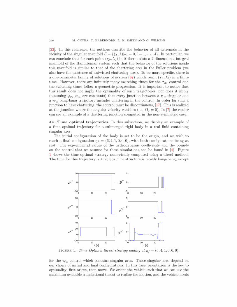
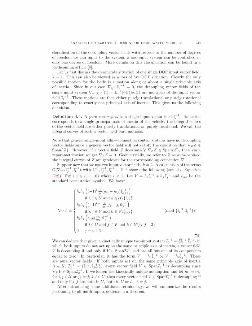
3.5. Time optimal trajectories. In this subsection, we display an example ofa time optimal trajectory for a submerged rigid body in a real fluid containingsingular arcs.
The initial configuration of the body is set to be the origin, and we wish toreach a final configuration ηf = (6, 4, 1, 0, 0, 0), with both configurations being atrest. The experimental values of the hydrodynamic coefficients and the boundson the control that we assume for these simulations can be found in [4]. Figure1 shows the time optimal strategy numerically computed using a direct method.The time for this trajectory is ≈ 25.85s. The structure is mostly bang-bang, except
0 10 20−10
0
10
γ ν 1
0 10 20−10
0
10
γ ν 2
0 10 20−20
0
20
40
γ ν 3
t (s)
0 10 20−5
0
5
γ Ω1
0 10 20−5
0
5
γ Ω2
0 10 20−1
0
1
γ Ω3
t (s)
Figure 1. Time Optimal thrust strategy ending at ηf = (6, 4, 1, 0, 0, 0).
for the τΩ3 control which contains singular arcs. These singular arcs depend onour choice of initial and final configurations. In this case, orientation is the key tooptimality; first orient, then move. We orient the vehicle such that we can use themaximum available translational thrust to realize the motion, and the vehicle needs
ANALYSIS OF TRAJECTORY DESIGN FOR UNDERWATER VEHICLES 247
to maintain this orientation over the entire trajectory. Singular arcs do not appearin τΩ1 and τΩ2 because their full power is needed to offset the righting moments.The translational controls ϕν1,ν2,ν3 are used to their full extent, as one would expectfor a time optimal translational displacement.
4. Kinematic motions. In terms of affine differential geometry, Proposition 4has important consequences. Indeed, there is a relation between our result andthe existence of kinematic motions along decoupling vector fields. This is what weestablish in this section.
We consider a rigid body moving in an ideal fluid (air). Moreover, we makethe following additional assumptions. We assume CG coincides with CB . Since wealso assume the vehicle to be neutrally buoyant, there are no restoration forces ormoments acting on the vehicle. In other words, the system is void of external forces.
We remind the reader of the notation introduced in section 2; we use mi =m+Mνi
f and ji = Ibi+ JΩi
f . As we will see, our results depend on the symmetriesof the rigid body, hence we introduce some terminology.
Definition 4.1. We call our system kinetically unique if all the eigenvalues in thekinetic energy metric G are distinct.
In particular, Definition 4.1 implies that for a kinetically unique system the addedmass (mi) and added mass moment of inertia (ji) coefficients are all distinct. Sincethe added mass is a measure of the fluid that must be accelerated with the body,unique mi’s imply that the view of the body along each body-frame axis is different.Note that you can have 3 axes of symmetry with 3 unique added mass coefficients,as is the case with an ellipsoidal body with three distinct axis lengths. Unique ji’simply a nonuniform mass distribution for the body. In practice, this is generallythe case.
Under our assumptions, the equations of motion have the form:
∇γ ′γ ′ =
6∑
i=1
σi(t)I−1i (γ(t)). (69)
In the sequel we denote by I−1 the set of input vector fields to our system: I−1 =I
−11 , . . . , I−1
6 . We note here that under our assumptions, I−1 is diagonal, and thuseach I
−1i , i = 1, ..., 6, is a single degree of freedom input to the system.
Definition 4.2. We refer to I−1i , i ∈ U as the translational control vector fields and
I−1j , j ∈ V as the rotational control vector fields.
4.1. Decoupling vector fields. In this paper we are interested in kinematic re-ductions of rank one for the system in (69); namely decoupling vector fields. Let usfirst introduce some definitions and terminology.
Suppose we have a general affine-connection control system given by
∇γ ′(t)γ′(t) =
k∑
a=1
ua(t)Za(γ(t)), (70)
where u1(t), . . . , uk(t) are measurable controls and Z1, . . . , Zk is a set of locallydefined independent vector-fields on the configuration space M whose images lie ina rank-k smooth distribution Z ⊂ TM .
248 M. CHYBA, T. HABERKORN, R. N. SMITH AND G. WILKENS
Definition 4.3 (see [2]). A decoupling vector field for an affine-connection controlsystem is a vector field V on M having the property that every reparametrizedintegral curve for V is a trajectory for the affine-connection control system. Moreprecisely, let γ : [0, S] → M be a solution for γ ′(s) = V (γ(s)) and let s : [0, T ] →[0, S] satisfy s(0) = s′(0) = s′(T ) = 0, s(T ) = S, s′(t) > 0 for t ∈ (0, T ), and(γ s)′ : [0, T ] → TM is absolutely continuous. Then γ s : [0, T ] → M is atrajectory for the affine-connection control system. Additionally, an integral curveof V is called a kinematic motion for the affine-connection control system.
A necessary and sufficient condition for V to be a decoupling vector field for theaffine-connection control system (70) is that both V and ∇V V are sections of Z [2,p. 426]. Notice that if Z = TM (i.e. (70) is fully-actuated) then every vector fieldis a decoupling vector field, and if Z has rank k = 1 (i.e. (70) is single-input) thenV is a decoupling vector field if and only if both V and ∇V V are multiples of Z1.
In the under-actuated setting, decoupling vector fields are found by solving asystem of homogeneous quadratic polynomials in several variables. Given a vector
field V , we must have that V =∑k
a=1 haZa since V ∈ Span Z1, . . . , Zk. Now,
since ∇V V ∈ Span Z1, . . . , Zk we want
∇V V = ∇∑haZa
∑hbZb ≡ 0 (mod Z). (71)
Starting with the middle of the above equation, we get that
∇∑haZa
∑hbZb =
∑ha∇Za
∑hbZb =
∑∑ha∇Za
(hbZb)
=∑∑
ha[Za(hb)Zb + hb∇ZaZb]
≡∑∑
hahb∇ZaZb (mod Z).
(72)
Thus, we are concerned with calculating ∇ZaZb for a, b ∈ 1, ..., k to find the
coefficients h1, . . . , hk such that V is decoupling.The equations of motion (69) for a submerged body in an ideal fluid are fully
actuated. As mentioned previously, in this case there are no quadratic polynomialsto solve and every left-invariant vector field is a decoupling vector field. However,the situation is not as straightforward in the under-actuated scenario; practicallyspeaking, the case of actuator failure. In this situation, the body may be unableto apply a force or torque in one or more of the six DOF, limiting the vehicle’scontrollability. This is an interesting case because it is likely that an underwatervehicle loses actuator power for one reason or another but still needs to move. Forexample, we would like the vehicle to be able to return home in a distressed situation.Decoupling vector fields give possible trajectories for the return home which thevehicle is able to realize in an under-actuated condition. In [3], the authors consideran under-actuated situation that differs from the ones we are considering here (theyassume three body-fixed control forces that are applied at a point different from thecenter of gravity). Here we assume that actuator failure results in the ability tocontrol less than six DOF.
In other words, we consider the under-actuated systems
∇γ ′(t)γ′(t) =
k∑
i=1
σi(t)I−1i (γ(t)), (73)
with k < 6, I−11 , . . . , I−1
k an independent subset of I−1, and σ1, . . . , σk the cor-
responding controls; see (16). We define I−1k = I
−11 , . . . , I−1
k . We first give a
ANALYSIS OF TRAJECTORY DESIGN FOR UNDERWATER VEHICLES 249
classification of the decoupling vector fields with respect to the number of degreesof freedom we can input to the system; a one-input system can be controlled inonly one degree of freedom. More details on this classification can be found in aforthcoming article [8].
Let us first discuss the degenerate situation of one single DOF input vector field,k = 1. This can also be viewed as a loss of five DOF situation. Clearly the onlypossible motion for the body is a motion along or about a single principle axisof inertia. Since in our case ∇Ii
−1Ii−1 = 0, the decoupling vector fields of the
single input system ∇γ ′(t)γ′(t) = Ii
−1(γ(t))σi(t) are multiples of the input vector
field Ii−1. These motions are then either purely translational or purely rotational
corresponding to exactly one principal axis of inertia. This gives us the followingdefinition.
Definition 4.4. A pure vector field is a single input vector field I−1i . Its action
corresponds to a single principal axis of inertia of the vehicle; the integral curvesof the vector field are either purely translational or purely rotational. We call theintegral curves of such a vector field pure motions.
Note that generic single-input affine-connection control systems have no decouplingvector fields since a generic vector field will not satisfy the condition that ∇ZZ ∈SpanZ. However, if a vector field Z does satisfy ∇ZZ ∈ SpanZ, then via areparametrization we get ∇ZZ = 0. Geometrically, we refer to Z as auto-parallel ;the integral curves of Z are geodesics for the corresponding connection ∇.
Suppose now that we use two input vector fields; k = 2. A calculation of the termsG(∇
I−1i
I−1j , I−1
k ) with I−1i , I−1
j , I−1k ∈ I−1 shows the following (see also Equation
(72)). Fix i, j ∈ 1, ..., 6 where i < j. Let V = hi I−1i + hj I
−1j and ǫijk be the
standard permutation symbol. We have:
∇V V ≡
hihj
((−1)k 1
jk(mi −mj)I
−1k+3
)
if i, j ∈ U and k ∈ U\i, jhihj
((−1)k+1 1
jk(jj − ji)I
−1k
)
if i, j ∈ V and k ∈ V\i, jhihj
(ǫijk( mi
mk)I−1
k
)
if i ∈ U and j ∈ V and k ∈ U\i, j − 30 j = i+ 3
(mod I−1i , I−1
j )
(74)
We can deduce that given a kinetically unique two-input system I−12 = I
−11 , I−1
2 inwhich both inputs do not act upon the same principle axis of inertia, a vector fieldV is decoupling if and only if V ∈ SpanI−1
2 and has all but one of its components
equal to zero. In particular, it has the form V = h1I−11 or V = h2I
−12 . These
are pure vector fields. If both inputs act on the same principle axis of inertia(i ∈ U , I−1
2 = I−1i , I−1
3+i), every vector field V ∈ SpanI−12 is decoupling since
∇V V ∈ SpanI−12 . If we loosen the kinetically unique assumption and let mi = mj
for i, j ∈ U or jk = jl k, l ∈ V , then every vector field V ∈ SpanI−12 is decoupling if
and only if i, j are both in U , both in V or i+ 3 = j.After introducing some additional terminology, we will summarize the results
pertaining to all mutli-inputs systems in a theorem.
250 M. CHYBA, T. HABERKORN, R. N. SMITH AND G. WILKENS
Definition 4.5. A vector field V is called an axial vector field if it is of the formV = hi I
−1i + hi+3 I
−1i+3 where i ∈ U .
We use the term axial motions since the corresponding kinematic motions are atranslation and rotation acting on the same principle axis of inertia. We call theseintegral curves axial motions. They can be seen as an extension of the pure motions.
Definition 4.6. A vector field V is called a coordinate vector field if it is of theform V = hi I
−1i + hj I
−1j + hk I
−1k where i = 1 or 4, j = 2 or 5 and k = 3 or 6.
We choose the term coordinate vector field since all three principal axes of theinertial coordinate frame are represented. A kinematic motion for such a vector isreferred to as a coordinate motion.
Theorem 4.7. Under our assumptions on a submerged rigid body in an ideal fluidwe have the following characterization for the decoupling vector fields in terms ofthe number of degrees of freedom we can input to the system.
Case 1:: Single-input system, I−11 = I
−11 . The decoupling vector fields are
multiples of I−11 ; these are pure vector fields.
Case 2:: Two-input system, I−12 = I
−11 , I−1
2 in which both inputs do not actupon the same principle axis of inertia. Then, for a kinetically unique system,a vector field V ∈ SpanI−1
2 is decoupling if and only if V has all but one of
its components equal to zero. In particular, it has the form V = h1 I−11 or
V = h2 I−12 ; these are pure vector fields. If the input vector fields act on the
same principal axis of inertia, then every vector field in SpanI−12 is decoupling.
Assuming mi = mj for i, j ∈ U or jk = jl k, l ∈ V, then every vector field
V ∈ SpanI−12 is decoupling if and only if i, j are both in U or both in V or
i+ 3 = j.Case 3:: Three-input system.
1. Three Translational Inputs: I−13 = I
−11 , I−1
2 , I−13 . For a kinetically
unique system, a vector field V ∈ SpanI−13 is decoupling if and only if
V has all but one of its components equal to zero. In particular, it has theform V = hi I
−1i for i ∈ U ; these are the pure translational vector fields.
Assuming exactly two of the mi’s are equal, we get the axial vector fieldsas additional decoupling vector fields: V = hi I
−1i +hj I
−1j , where mi = mj
and mi 6= mk. If mi = mj = mk, then every vector field V ∈ SpanI−13 is
decoupling since in this case ∇V V ∈ SpanI−13 .
2. Three Rotational Inputs: I−13 = I
−14 , I−1
5 , I−16 . In this situation ∇V V ∈
SpanI−13 for all V ∈ SpanI−1
3 , thus each vector field V ∈ SpanI−13 is
decoupling.3. Mixed Translational and Rotational Inputs. Suppose we have a kinetically
unique three input system such that the inputs are not all translationalor all rotational but represents motions along three distinct axis. In thecase that two inputs are translational, every vector field V ∈ SpanI−1
3
is decoupling. In the case that two inputs are rotational, the decouplingvector fields are the pure vector fields V ∈ SpanI−1
3 . Suppose we havea kinetically unique three input system such that the inputs are not alltranslational or all rotational but represents motions along only two dis-tinct axis: I−1
3 = Ii, Ii+3, Ij, i ∈ U , j 6= i, i+ 1. The decoupling vector
fields are the axial vector fields, V = hi I−1i + hi+3 I
−1i+3 for i ∈ U , and the
ANALYSIS OF TRAJECTORY DESIGN FOR UNDERWATER VEHICLES 251
pure vector fields, V = hj I−1j . The remarks about the symmetries in the
case of three translational input are valid in this case also.Case 4:: Four input system.
1. Three Translation, One Rotation: I−14 = I
−11 , I−1
2 , I−13 , I−1
k where k ∈V. For a kinetically unique system the decoupling vector fields are theaxial vector fields V = hk−3 I
−1k−3 + hk I
−1k or the coordinate vector fields
V = hi I−1i + hj I
−1j + hk I
−1k with i, j ∈ U , i, j 6= k − 3. If mk−3 = mi
for i ∈ U and i 6= k − 3, then V = hi I−1i + hk−3 I
−1k−3 + hk I
−1k is also a
decoupling vector field. If m1 = m2 = m3, then every vector field V ∈ I−1
is a decoupling vector field.2. Three Rotations, One Translation: I−1
4 = I−1i , I−1
4 , I−15 , I−1
6 where i ∈U . Then the decoupling vector fields are the axial vector fields V = hi I
−1i +
hi+3 I−1i+3 or the coordinate vector fields V = h4 I
−14 + h5 I
−15 + h6 I
−16 .
3. Two Translations, Two Rotations. For a kinetically unique system, if twoprinciple axes are repeated: I−1
4 = I−1i , I−1
j , I−1i+3, I
−1j+3 where i, j ∈ U ,
then the decoupling vector fields are either the pure vector fields V =ha I−1
a for a ∈ i, j, i + 3, j + 3 or the axial vector fields V = ha I−1a +
ha+3 I−1a+3 where a = 1 or a = j. If mi = mj, then additional de-
coupling vector fields for the system are V = hi I−1i + hj I
−1j + hk I
−1k
where k = i + 3 or k = j + 3. And, if ji = jj, then additional de-
coupling vector fields for the system are of the form V = hi+3 I−1i+3 +
hj+3 I−1j+3. For a kinetically unique system, if one principle axis is re-
peated: I−14 = I
−1i , I−1
j , I−1i+3, I
−1k+3 where i, j, k ∈ U , then the decou-
pling vector fields are the axial vector fields V = hi I−1i + hi+3 I
−1i+3 or
the coordinate vector fields V = hi I−1i + hj I
−1j + hk+3 I
−1k+3. If ji = jk
then hj or hi+3 must be zero, and additional decoupling vector fields are
V = hi I−1i + hi+3 I
−1i+3 + hk+3 I
−1k+3.
Case 5:: Five input system.1. Three Translations, Two Rotations: I−1
5 = I−11 , I−1
2 , I−13 , I−1
i , I−1j where
i, j ∈ V, and let k ∈ V such that k 6= i or j. For a kinetically uniquesystem the decoupling vector fields are V = ha I−1
a +ha+3 I−1a+3 +hk−3 I
−1k−3
where a ∈ U−(k−3) and the coordinate vector fields V = ha I−1a +hb I
−1b +
hk−3 I−1k−3 where a, b ∈ U−(k−3).Assuming that mi−3 = mj−3, additional
decoupling vector fields are given by V = ha I−1a +hk I
−1k +hi I
−1i +hj I
−1j
where a = i − 3 or a = j − 3 and k ∈ U − i − 3, j − 3. Assumingthat ji−3 = jj−3, additional decoupling vector fields are given by V =
h1 I−11 + h2 I
−12 + h3 I
−13 + ha I−1
a where a = i or a = j.2. Two Translations, Three Rotations: I−1
5 = I−1i , I−1
j , I−14 , I−1
5 , I−16 where
i, j ∈ U , and let k ∈ U such that k 6= i or j. For a kinetically uniquesystem the decoupling vector fields are V = ha I−1
a +ha+3 I−1a+3 +hk+3 I
−1k+3
where a ∈ V − (k + 3), the coordinate vector fields V = ha I−1a + hb I
−1b +
hk+3 I−1k+3 where a, b ∈ V − (k + 3) and the coordinate vector fields V =
hiI−1i + hjI
−1j + haI−1
a where a ∈ V −i+ 3, j+ 3. Loosening the kineticuniqueness assumption does not provide any additional decoupling vectorfields in this case.
Case 6:: Six input system. Every vector field is decoupling.
252 M. CHYBA, T. HABERKORN, R. N. SMITH AND G. WILKENS
The major application of computing decoupling vector fields is the design oftrajectories for our system. This is addressed in the following section.
4.2. Motion planning. In this section, we present an approach to design trajec-tories for our mechanical system based on the theory developed in the previoussections. A similar technique applied to two specific systems can be found in [3].Based on Theorem 4.7, we give partial answers to the motion planning problemfor the under-actuated scenarios considered in Section 4.1. By using kinematicmotions to design trajectories, we reduce the order of the dynamic system underconsideration.
Another method for constructing kinematic controls for under-actuated mechan-ical systems defined using a geometric architecture can be found in [13, 15, 16]and the references contained therein. The cited authors propose small-amplitude,low-frequency, periodic time-varying controls with which to maneuver the chosenmechanical system. This approach differs from the technique described here in twomain ways. First, the sinusoidal controls solve the motion planning problem for thekinematic system, but may not necessarily be solutions to the considered dynamicsystem. Computing the controls from the concatenations of integral curves of decou-pling vector fields via inverse kinematics guarantees that these controls are in factsolutions to the dynamic system. The other difference comes in the implementabil-ity of the computed controls onto a test-bed AUV. Although implementable (see[14]), the small-amplitude, low-frequency, periodic time-varying controls are onlyapplicable to vehicles operating at low Reynolds number (< 103). Also, in an effortto reduce errors created by non-linearities inherent to the physical thrusters, it isuseful to reduce the number of switching times for these actuators; this directlyopposes the implementation of periodic (about zero) controls. These main differ-ences motivate the development of kinematic controls which are also solutions tothe dynamic system and can be implemented over larger operational velocities.
The motion planning problem for the submerged rigid body is the following.Given an initial configuration q0 ∈ Q and a final configuration q1 ∈ Q both beingat rest (i.e. qo, q1 have zero velocity), produce a trajectory that steers the systemfrom q0 to q1. For simplicity we assume in the sequel that the initial configurationis always the origin.
A first obvious remark is that if we have control on all six DOF (i.e. we arefully actuated), we can reach any configuration from our initial configuration by aconcatenation of pure motions. At the other extreme, with only one input vectorfield the rigid body is restricted to movement in only one degree of freedom. Aninteresting question is the minimal number of inputs which we need in order toreach any configuration from the origin using exclusively kinematic motions. Butbefore we address that question, let us introduce some terminology.
Definition 4.8. A submerged rigid body in an ideal fluid is said to be kinematicallycontrollable if every point in the configuration space SE(3) is reachable from theorigin via a sequence of kinematic motions.
Notice that we can reparametrize each kinematic motion to satisfy boundaryconstraints on the controls, and to begin and end at rest. Hence, in what follows,we assume that each kinematic motion starts and ends at rest. The main objective ofthis section is to determine how many input vector fields, each controlling one degreeof freedom, are needed to provide enough decoupling vector fields for kinematiccontrollability. We begin with the following obvious lemma.
ANALYSIS OF TRAJECTORY DESIGN FOR UNDERWATER VEHICLES 253
Lemma 4.9. If a rigid body submerged in an ideal fluid is kinematically controllable,it cannot be controlled by only translational motions or only rotational motions.
Corollary 1. A submerged rigid body in an ideal fluid is not kinematically con-trollable if there is only a single input control vector field: I
−11 . The same is true
if there are only two input control vector fields I−12 = I
−1i , I−1
j with i, j ∈ U or
i, j ∈ V, or three input vector fields I−13 = Ii, Ij , Ik with i, j, k all in U or all in
V.
Proof. If all inputs are translational, then ηf = (0, 0, 0, φ0, θ0, ψ0) is unreachablesince we cannot control rotation. Similarly if all inputs are rotational, the vehiclecannot reach ηf = (a, b, c, 0, 0, 0) since we do not control translation.
To check the other cases, we will use the following result.
Theorem 4.10. Consider an underactuated rigid body submerged in an ideal fluid:
∇γ ′(t)γ′(t) =
k∑
i=1
σi(t)I−1i (γ(t)), (75)
with k < 6, I−11 , . . . , I−1
k an independent subset of I−1, and denote by X a set ofdecoupling vector fields. Suppose that the involutive closure of X , denoted by LieX ,span the tangent space T SE(3). Then, the system is kinematically controllable.
Proof. Following our construction, we have reduced the motion planning for theunderactuated system to computing integral curves of single-input driftless systemsdefined on the configuration manifold SE(3). The theorem is then a consequenceof a well-known generalization of Chow’s theorem. This generalization ensuresthe controllability of a driftless system using only the integral curves of the inputvector fields. See [2, Thm. 13.2] for instance. Global controllability follows fromthe connectedness of SE(3).
In order to determine whether our system is kinematically controllable we willneed to determine the involutive closure of the set of decoupling vector fields. Thefollowing shows the procedure used for computing Lie brackets to find the involutiveclosure. Since we have Q = SE(3), the linear space of body-fixed velocities is theLie algebra se(3):
se(3) = [0 0
ν Ω
]|ν ∈ R
3, Ω ∈ R3. (76)
If ζ = (ν,Ω)t represents the body-fixed velocity, we let [ζ, η] denote the Lie bracketoperation on se(3). Given ζ ∈ se(3), we define the adjoint operator adζ : se(3) →se(3) as adζ η = [ζ, η]. Because
[[0 0
ν1 Ω1
],
[0 0
ν2 Ω2
]]=
[0 0
Ω1ν2 − Ω2ν1 Ω1Ω2 − Ω2Ω1
], (77)
and since (ν,Ω) ∈ R3 × R3 ∼= se(3) we can write
[(ν1,Ω1), (ν2,Ω2)] = (Ω1 × ν2 − Ω2 × ν1,Ω1 × Ω2). (78)
Thus, we can define the adjoint operator ad(ν,Ω) : se(3) → se(3) as ad(ν1,Ω1)(ν2,Ω2) =[(ν1,Ω1), (ν2,Ω2)] and as a linear transformation is represented by the matrix
ad(ν,Ω) =
[Ω ν
0 Ω
]. (79)
254 M. CHYBA, T. HABERKORN, R. N. SMITH AND G. WILKENS
Thus, over this matrix Lie group, the operation of Lie bracket is the same as the ma-trix commutator. This formulation allows the computation of Lie brackets withoutdifferentiation.
Now we are ready to display the results.
Lemma 4.11. Given any two translational control vector fields I−1i , I−1
j , i, j ∈ U ,
their Lie bracket vanishes: [I−1i , I−1
j ] = 0. Given two distinct rotational control
vector fields I−1i , I−1
j , i, j ∈ V, their Lie bracket produces the third rotational
control vector field I−1k , k ∈ V , k 6= i, j.
Proof. Computational.
Theorem 4.12. If the set of decoupling vector fields contain only one translationalcontrol vector field and one rotational control vector field, the kinematic motionsof the rigid body are restricted to a plane in R3. Thus, a submerged rigid bodyin an ideal fluid with only two control vector fields I
−1i , I−1
j is not kinematicallycontrollable.
Proof. If i, j ∈ U or i, j ∈ V then we are done by Corollary 1. Thus, suppose thetwo inputs are I
−1i and I
−1j where i ∈ U and j ∈ V . Now consider L = [I−1
i , I−1j ].
For j = i + 3, L = 0 since both inputs act on the same axis. If j 6= i + 3, thenL = I
−1k where k ∈ U and i 6= k 6= (j − 3). Thus, the movement for a two input
system is restricted to kinematic motion associated to SpanI−1i , I−1
j , I−1k where
i, k ∈ U , j ∈ V and i 6= k 6= (j − 3). This defines a plane in R3.
Theorem 4.13. Assume the set of decoupling vector fields is the span of threetranslational control vector field and one rotational control vector field. Then, it isnot kinematically controllable.
Proof. Assume that the vector fields I−11 , I−1
2 , I−13 , I−1
k , where k ∈ V form a setof generators for the set of decoupling vector fields. From the computations in theproof of Theorem 4.12 we know that for i ∈ U and j ∈ V
[I−1i , I−1
j ] =
0 j = i+ 3
I−1l l ∈ U and i 6= l 6= j
. (80)
Hence, if we denote by W the involutive closure of the set of control vector fieldswe have that W is a strict subset of the tangent space. Since in the analytic spaceChow’s condition is sufficient and necessary, see [1] for instance, we can concludethat the system is not controllable and hence not kinematically controllable.
Remark 7. In the situation of Theorem 4.13, the vehicle is able to reach any desiredposition in R3, but is unable to reach any orientation in SE(3). In particular, thevehicle is unable to realize ηf = (0, 0, 0, φ0, θ0, ψ0) from the origin if φ0 or θ0 arenon-zero.
Corollary 2. A three-input rigid body submerged in an ideal fluid with two transla-tional and one rotational input is not kinematically controllable. A four input rigidbody submerged in an ideal fluid with only one rotational input vector field is notkinematically controllable.
Proof. This is a consequence of Theorem 4.13.
ANALYSIS OF TRAJECTORY DESIGN FOR UNDERWATER VEHICLES 255
Theorem 4.14. If the set of decoupling vector fields contains at least one transla-tional control vector field and two distinct rotational control vector fields, then thesubmerged rigid body in an ideal fluid is kinematically controllable.
Proof. Assume that the decoupling vector fields for our system contain the vectorfields I
−1i , I−1
j , I−1k where i ∈ U , j, k ∈ V and i < j < k. An easy computation
shows that I−1i , I−1
j , I−1k , [I−1
i , I−1k ], [I−1
j , I−1k ], [[I−1
i , I−1k ], [I−1
j , I−1k ]] are six linearly
independent vectors which span R6. Thus, there exists a path between any two zerovelocity configurations through the concatenation of integral curves of decouplingvector fields for which each segment is reparametrized to start and end at zerovelocity.
Corollary 3. If the set of decoupling vector fields contains a coordinate vector fieldV = hiI
−1i + hjI
−1j + hkI
−1k , where i ∈ U and j, k ∈ V, then the submerged rigid
body in an ideal fluid is kinematically controllable.
Corollary 4. A three input rigid body submerged in an ideal fluid with one trans-lational and two rotational input is kinematically controllable. A four input rigidbody submerged in an ideal fluid with at least two rotational inputs vector fields iskinematically controllable. A m input rigid body submerged in an ideal fluid withm ∈ 5, 6 is kinematically controllable.
Proof. This is a consequence of Theorem 4.7 and Theorem 4.13.
We now wish to apply the results of this section to the motion planning of realAUVs. The majority of AUVs are controlled using external thrusters, which do notact directly at CG, and possibly movable wings, foils or rudders. Since actuation ofmovable wings, foils and rudders implies an applied force or torque to the vehicle,without loss of generality, we can assume that the vehicle is controlled strictly viaexternal thruster actuation. This assumption will also make the following exampleseasier to visualize. We shall call a thruster oriented such that the output forceis parallel to the (body-frame) z-axis a vertical thruster, and a thruster orientedsuch that the output force is perpendicular to the (body-frame) z-axis a horizontalthruster. Clearly, a vertical thruster contributes to heave, roll and pitch controls,while a horizontal thruster contributes to surge, sway and yaw controls.
Suppose we begin with a fully-actuated submersible which controls heave, rolland pitch with one set thrusters we will call V. While surge, sway, and yaw arecontrolled with another set of thrusters called H. In order to utilize the notion ofdecoupling vector fields in the under-actuated situation, suppose we lose the abilityto control either H or V. From Theorem 4.13, losing V would limit the motion of thevehicle to a plane. However, losing H would not affect the kinematic controllabilityof the vehicle by the result of Theorem 4.16. Thus, in the design process of thevehicle, we could save money by requiring that robustness or redundancy need onlybe implemented onto a portion of the system; the V thrusters. Also, for energyconservation, it may be better to use only one set of thrusters to save battery life.This knowledge and ability to pre-plan can save time and money for the AUVdesigner and end-user alike.
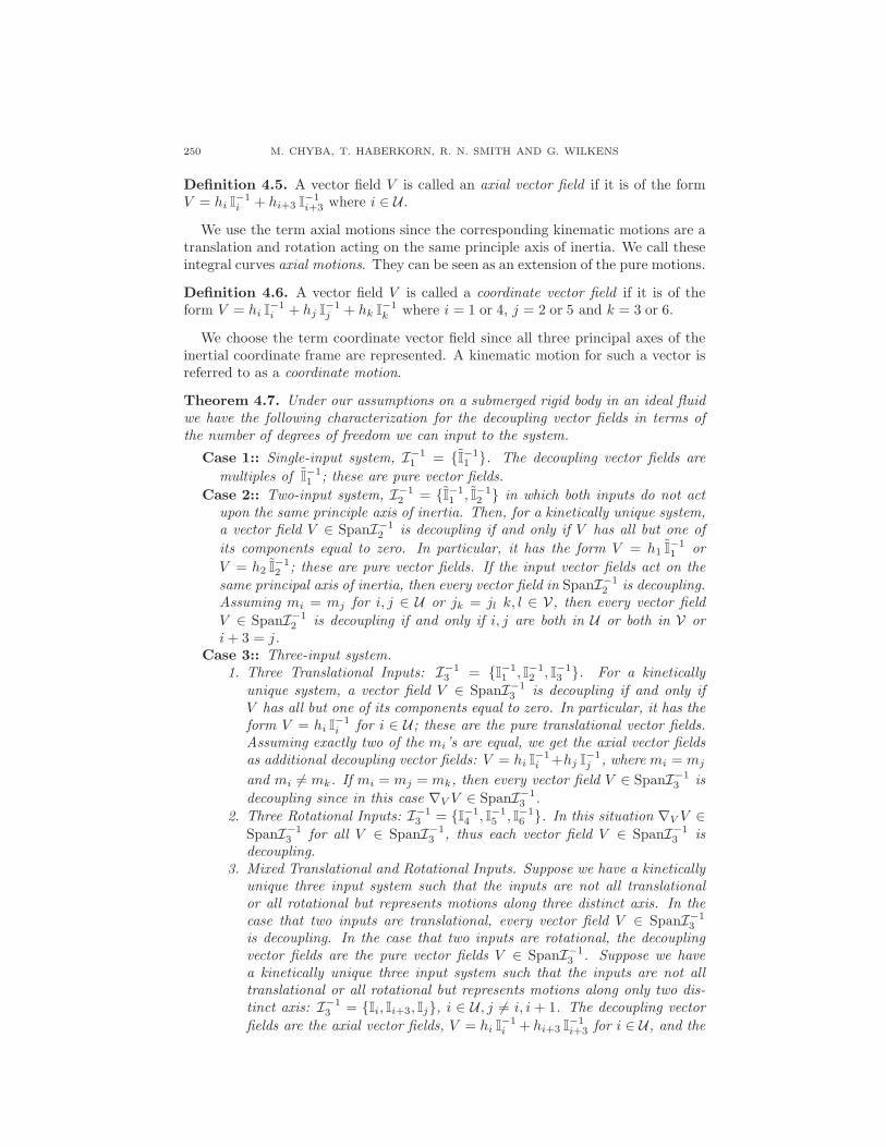
Now, we demonstrate two practical applications to summarize the results of thissection. Suppose that we want to start at the origin (η0 = (0, 0, 0, 0, 0, 0)) and endat ηf = (4, 3, 2, 0, 0,−90). Positive b3 values are in the direction of gravity. In thefirst scenario, suppose we have a vehicle designed as above. Also suppose that weare only able to control the V thrusters. In particular, we are only able to directly
256 M. CHYBA, T. HABERKORN, R. N. SMITH AND G. WILKENS
control heave, roll and pitch, and the input vector fields are I−13 = I
−13 , I−1
5 , I−16 .
By Theorem 4.16, the vehicle is kinematically controllable, and by Theorem 4.7 weknow that the decoupling vector fields for this system are the pure vector fields,V = hiI
−1i for i ∈ 3, 5, 6. This means that the trajectory can be fully decoupled
into a concatenation of pure motions. The basic idea to realize this displacement isuse the pitch and roll controls to point the bottom of the vehicle in the directionof ηf and then use pure heave for the translational displacement. Upon reaching(4, 3, 2, φ, θ, ψ) we can do pitch and roll movements to realize ηf . For this example,the vehicle needs to apply a pure pitch to reach tan−1(3
2 ) = 56.3, pure roll to
reach − tan−1(2) = −63.4, then translate√
22 +√
42 + 32 = 3 units using pureheave. Now, the vehicle has position η = (4, 3, 2,−63.4, 56.3, 0). To reach ηf
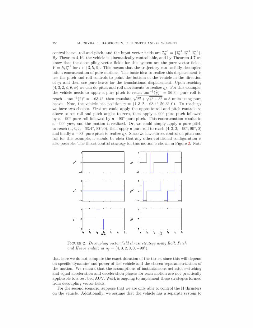
we have two choices. First we could apply the opposite roll and pitch controls asabove to set roll and pitch angles to zero, then apply a 90 pure pitch followedby a −90 pure roll followed by a −90 pure pitch. This concatenation results ina −90 yaw, and the motion is realized. Or, we could simply apply a pure pitchto reach (4, 3, 2,−63.4, 90, 0), then apply a pure roll to reach (4, 3, 2,−90, 90, 0)and finally a −90 pure pitch to realize ηf . Since we have direct control on pitch androll for this example, it should be clear that any other rotational configuration isalso possible. The thrust control strategy for this motion is shown in Figure 2. Note
Figure 2. Decoupling vector field thrust strategy using Roll, Pitchand Heave ending at ηf = (4, 3, 2, 0, 0,−90).
that here we do not compute the exact duration of the thrust since this will dependon specific dynamics and power of the vehicle and the chosen reparametrization ofthe motion. We remark that the assumptions of instantaneous actuator switchingand equal acceleration and deceleration phases for each motion are not practicallyapplicable to a test bed AUV. Work is ongoing to implement these strategies formedfrom decoupling vector fields.
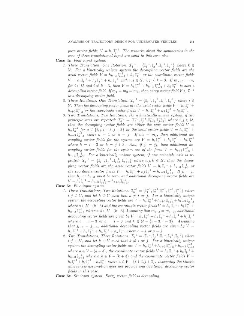
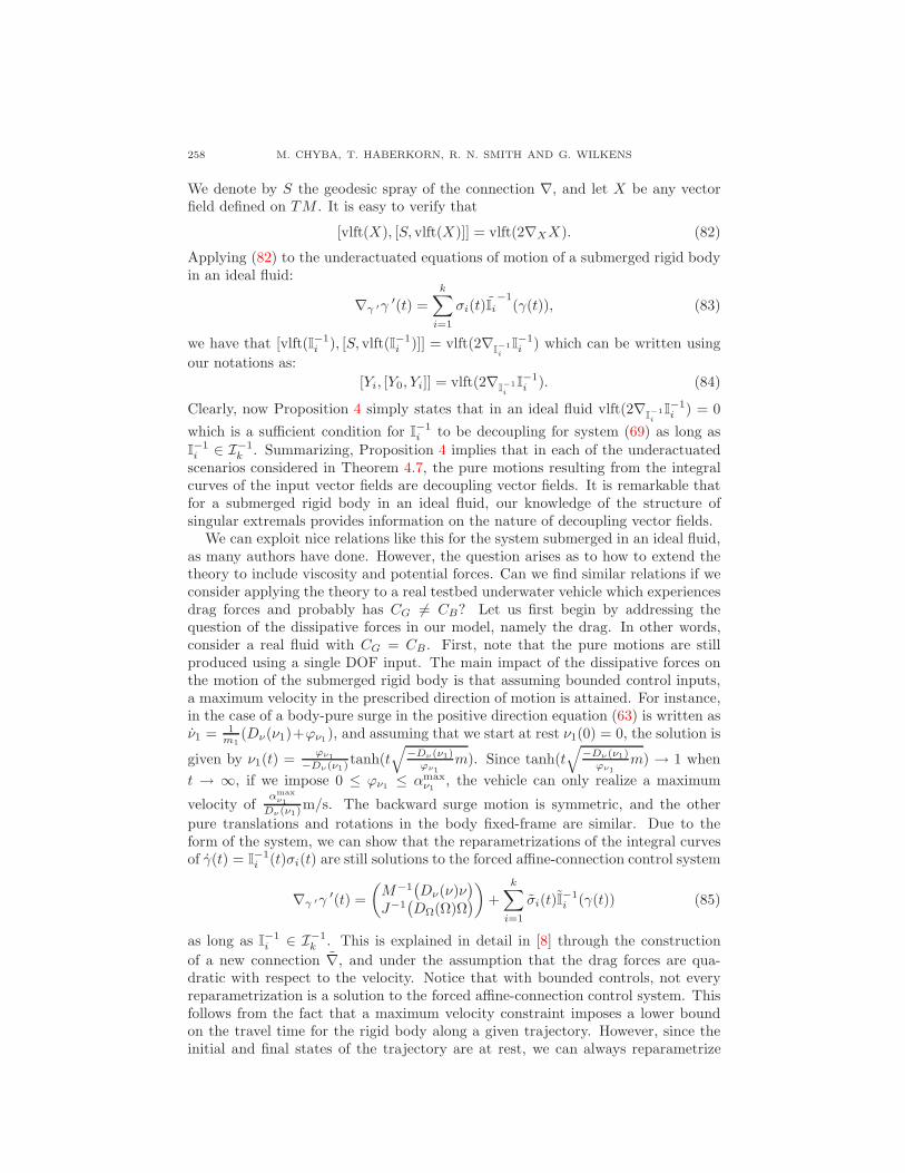
For the second scenario, suppose that we are only able to control the H thrusterson the vehicle. Additionally, we assume that the vehicle has a separate system to
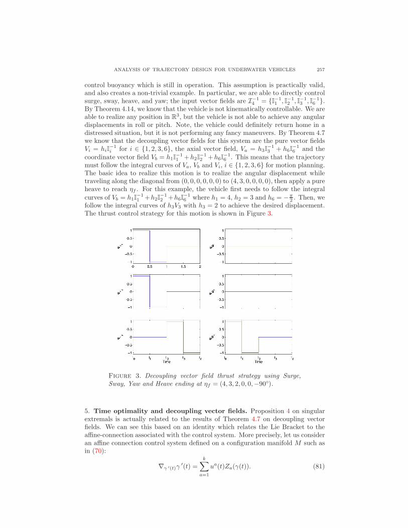
ANALYSIS OF TRAJECTORY DESIGN FOR UNDERWATER VEHICLES 257
control buoyancy which is still in operation. This assumption is practically valid,and also creates a non-trivial example. In particular, we are able to directly controlsurge, sway, heave, and yaw; the input vector fields are I−1
4 = I−11 , I−1
2 , I−13 , I−1
6 .By Theorem 4.14, we know that the vehicle is not kinematically controllable. We areable to realize any position in R3, but the vehicle is not able to achieve any angulardisplacements in roll or pitch. Note, the vehicle could definitely return home in adistressed situation, but it is not performing any fancy maneuvers. By Theorem 4.7we know that the decoupling vector fields for this system are the pure vector fieldsVi = hiI
−1i for i ∈ 1, 2, 3, 6, the axial vector field, Va = h3I
−13 + h6I
−16 and the
coordinate vector field Vb = h1I−11 +h2I
−12 +h6I
−16 . This means that the trajectory
must follow the integral curves of Va, Vb and Vi, i ∈ 1, 2, 3, 6 for motion planning.The basic idea to realize this motion is to realize the angular displacement whiletraveling along the diagonal from (0, 0, 0, 0, 0, 0) to (4, 3, 0, 0, 0, 0), then apply a pureheave to reach ηf . For this example, the vehicle first needs to follow the integral
curves of Vb = h1I−11 +h2I
−12 +h6I
−16 where h1 = 4, h2 = 3 and h6 = −π
2 . Then, wefollow the integral curves of h3V3 with h3 = 2 to achieve the desired displacement.The thrust control strategy for this motion is shown in Figure 3.
Figure 3. Decoupling vector field thrust strategy using Surge,Sway, Yaw and Heave ending at ηf = (4, 3, 2, 0, 0,−90).
5. Time optimality and decoupling vector fields. Proposition 4 on singularextremals is actually related to the results of Theorem 4.7 on decoupling vectorfields. We can see this based on an identity which relates the Lie Bracket to theaffine-connection associated with the control system. More precisely, let us consideran affine connection control system defined on a configuration manifold M such asin (70):
∇γ ′(t)γ′(t) =
k∑
a=1
ua(t)Za(γ(t)). (81)
258 M. CHYBA, T. HABERKORN, R. N. SMITH AND G. WILKENS
We denote by S the geodesic spray of the connection ∇, and let X be any vectorfield defined on TM . It is easy to verify that
[vlft(X), [S, vlft(X)]] = vlft(2∇XX). (82)
Applying (82) to the underactuated equations of motion of a submerged rigid bodyin an ideal fluid:
∇γ ′γ ′(t) =
k∑
i=1
σi(t)Ii
−1(γ(t)), (83)
we have that [vlft(I−1i ), [S, vlft(I−1
i )]] = vlft(2∇I−1i
I−1i ) which can be written using
our notations as:
[Yi, [Y0, Yi]] = vlft(2∇I−1i
I−1i ). (84)
Clearly, now Proposition 4 simply states that in an ideal fluid vlft(2∇I−1i
I−1i ) = 0
which is a sufficient condition for I−1i to be decoupling for system (69) as long as
I−1i ∈ I−1
k . Summarizing, Proposition 4 implies that in each of the underactuatedscenarios considered in Theorem 4.7, the pure motions resulting from the integralcurves of the input vector fields are decoupling vector fields. It is remarkable thatfor a submerged rigid body in an ideal fluid, our knowledge of the structure ofsingular extremals provides information on the nature of decoupling vector fields.
We can exploit nice relations like this for the system submerged in an ideal fluid,as many authors have done. However, the question arises as to how to extend thetheory to include viscosity and potential forces. Can we find similar relations if weconsider applying the theory to a real testbed underwater vehicle which experiencesdrag forces and probably has CG 6= CB? Let us first begin by addressing thequestion of the dissipative forces in our model, namely the drag. In other words,consider a real fluid with CG = CB. First, note that the pure motions are stillproduced using a single DOF input. The main impact of the dissipative forces onthe motion of the submerged rigid body is that assuming bounded control inputs,a maximum velocity in the prescribed direction of motion is attained. For instance,in the case of a body-pure surge in the positive direction equation (63) is written asν1 = 1
m1(Dν(ν1)+ϕν1), and assuming that we start at rest ν1(0) = 0, the solution is
given by ν1(t) =ϕν1
−Dν(ν1) tanh(t√
−Dν(ν1)ϕν1
m). Since tanh(t√
−Dν(ν1)ϕν1
m) → 1 when
t → ∞, if we impose 0 ≤ ϕν1 ≤ αmaxν1
, the vehicle can only realize a maximum
velocity ofαmax
ν1
Dν(ν1)m/s. The backward surge motion is symmetric, and the other
pure translations and rotations in the body fixed-frame are similar. Due to theform of the system, we can show that the reparametrizations of the integral curvesof γ(t) = I
−1i (t)σi(t) are still solutions to the forced affine-connection control system
∇γ ′γ ′(t) =
(M−1
(Dν(ν)ν
)
J−1(DΩ(Ω)Ω
))
+
k∑
i=1
σi(t)I−1i (γ(t)) (85)
as long as I−1i ∈ I−1
k . This is explained in detail in [8] through the construction
of a new connection ∇, and under the assumption that the drag forces are qua-dratic with respect to the velocity. Notice that with bounded controls, not everyreparametrization is a solution to the forced affine-connection control system. Thisfollows from the fact that a maximum velocity constraint imposes a lower boundon the travel time for the rigid body along a given trajectory. However, since theinitial and final states of the trajectory are at rest, we can always reparametrize

ANALYSIS OF TRAJECTORY DESIGN FOR UNDERWATER VEHICLES 259
a trajectory to accommodate the bound constraints on the controls. Here we domake the important assumption that the bounds on the controls are such that thevehicle can move through the fluid.
Up to this point we have kept the assumption that CG = CB. However, if therigid body is an underwater vehicle, this is not a desirable assumption. HavingCB and CG coincident is a neutral equilibrium, and hence very sensitive to anyexternal forces. Practically, we impose CG 6= CB in order to create a righting arm,and thus situating the vehicle in a stable equilibrium. In this situation, the vehiclewill restore pitch and roll angles from a listed configuration even if no control forceis applied. Thus, the effect of these restoring moments means that we may not beable to realize a body-pure motion with a single degree of freedom input controlvector field. As an example, let us consider a body-pure surge while maintaininga pitch angle of −45; a diagonal dive. Assuming CG = CB, we could first set theorientation, and then use a single control input to realize the motion. However,once we assume that CG 6= CB, we have to compensate for the induced rightingmoment by applying pitch control during the entire surge to maintain the desiredorientation. In general, we need to apply control to the pitch and roll angular veloc-ities to maintain the desired orientation and compensate for the righting momentswhile realizing a body-pure motion. Thus, at least three input control vectors arenow needed for a generic body-pure motion; pitch, roll and the prescribed directionof motion. In practice, four input control vector fields are usually controlled sothat one could compensate the righting moments and run a feedback control in yawto maintain the proper heading angle during the trajectory. However, there is norestoring moment in yaw and thus theoretically does not need to be directly con-trolled. If we additionally assume that the vehicle is not neutrally buoyant, we thenalso have to apply constant heave control in order to maintain a prescribed depth.With this additional assumption, we would need at least four input control vectorsto realize a body-pure motion. Notice that when considering bounded controls italso implies a controllability restriction due to the righting moments acting on theangular velocities. If the separation between CG and CB is large, the righting mo-ments will be significant and the vehicle may not be able to realize all orientationsin pitch and roll.
We summarize our remarks in the next proposition. In this proposition, a de-coupling vector field V is such that every reparametrization of its integral curves isa solution of the given forced affine-connection control system. Notice that we donot assume any bounds on the control for this proposition.
Proposition 6. Let ∇ be the affine connection (13) and consider the forced affineconnection control system
∇γ′γ′ =
(M−1
(Dν(ν)ν
)
J−1(DΩ(Ω)Ω − rB ×RtρgVk
))
+ Yiϕνi+
3∑
j=1
Yj+3τΩj,
where i ∈ U is fixed, and Yk = vlft(I−1k ). Then, every multiple of I
−1i is a decoupling
vector field for this system.If we consider the forced affine connection control system
∇γ′γ′ =
(M−1
(Dν(ν)ν
)
J−1(DΩ(Ω)Ω − rB ×RtρgVk
))
+3∑
j=1
Yj+3τΩj,
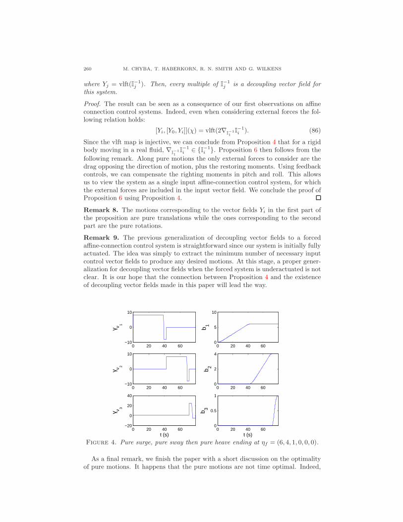
260 M. CHYBA, T. HABERKORN, R. N. SMITH AND G. WILKENS
where Yj = vlft(I−1j ). Then, every multiple of I
−1j is a decoupling vector field for
this system.
Proof. The result can be seen as a consequence of our first observations on affineconnection control systems. Indeed, even when considering external forces the fol-lowing relation holds:
[Yi, [Y0, Yi]](χ) = vlft(2∇I−11
I−1i ). (86)
Since the vlft map is injective, we can conclude from Proposition 4 that for a rigidbody moving in a real fluid, ∇
I−11
I−1i ∈ I
−1i . Proposition 6 then follows from the
following remark. Along pure motions the only external forces to consider are thedrag opposing the direction of motion, plus the restoring moments. Using feedbackcontrols, we can compensate the righting moments in pitch and roll. This allowsus to view the system as a single input affine-connection control system, for whichthe external forces are included in the input vector field. We conclude the proof ofProposition 6 using Proposition 4.
Remark 8. The motions corresponding to the vector fields Yi in the first part ofthe proposition are pure translations while the ones corresponding to the secondpart are the pure rotations.
Remark 9. The previous generalization of decoupling vector fields to a forcedaffine-connection control system is straightforward since our system is initially fullyactuated. The idea was simply to extract the minimum number of necessary inputcontrol vector fields to produce any desired motions. At this stage, a proper gener-alization for decoupling vector fields when the forced system is underactuated is notclear. It is our hope that the connection between Proposition 4 and the existenceof decoupling vector fields made in this paper will lead the way.
0 20 40 60−10
0
10
γ ν 1
0 20 40 60−10
0
10
γ ν 2
0 20 40 60−20
0
20
40
γ ν 3
t (s)
0 20 40 600
5
10
b 1
0 20 40 600
2
4
b 2
0 20 40 600
0.5
1
b 3
t (s)
Figure 4. Pure surge, pure sway then pure heave ending at ηf = (6, 4, 1, 0, 0, 0).
As a final remark, we finish the paper with a short discussion on the optimalityof pure motions. It happens that the pure motions are not time optimal. Indeed,
ANALYSIS OF TRAJECTORY DESIGN FOR UNDERWATER VEHICLES 261
using the maximum principle, it has been proven on a 2-dimensional model that eventhough pure motions are extremals (with the controls set to zero being singular)they are not time optimal, see [6]. Moreover, concatenation of pure motions throughconfigurations at rest eliminates their extremality property. Next, we compare apure motion trajectory to the optimal strategy for a submerged rigid body in areal fluid. We consider the 3D system with external forces. Figure 4 shows aconcatenated pure motion strategy; displaying only graphs of variables which arenot identically zero. The initial and final configurations are taken as in Section 3.5.Note that this trajectory is formed by a pure surge acceleration for tacc
surge ≈ 38.39
s, a deceleration for tdecsurge ≈ 3.74 s, a pure sway acceleration for tacc
sway ≈ 25.89
s, a deceleration for tdecsway ≈ 3.74 s, a pure heave acceleration for tacc
heave ≈ 2.92 s
and a deceleration for tdecheave ≈ 5.24 s. The non-symmetry of the acceleration and
deceleration phases is due to drag forces and physical actuator asymmetries (ourcomputations are based on a real underwater vehicle). The total transfer time forthis trajectory is tpure ≈ 79.92 s. This duration is more than triple the optimal time,see Figure 1. This is actually not that surprising since the pure motion trajectoryuses only a fraction of the available thrust at any given time.
REFERENCES
[1] B. Bonnard and M. Chyba, “Singular Trajectories and their Role in Control Theory,”Springer-Verlag, New York-Heidelberg-Berlin, 2003.
[2] F. Bullo and A. D. Lewis, “Geometric Control of Mechanical Systems Modeling, Analysis,and Design for Simple Mechanical Control Systems,” 49 in Texts in Applied Mathematics,Springer-Verlag, New York-Heidelberg-Berlin, 2005.
[3] F. Bullo and K. M. Lynch, Kinematic controllability for decoupled trajectory planning in
underactuated mechanical systems, IEEE Transactions. Robotics and Automation, 17 (2001),402–412.
[4] M. Chyba, T. Haberkorn, R. N. Smith and S. K. Choi, Design and implementation of time
efficient trajectories for autonomous underwater vehicles, Ocean Engineering, 35 (2007), 63–76.
[5] M. Chyba and T. Haberkorn, Autonomous underwater vehicles: singular extremals and chat-
tering, in “Proceedings of the 22nd IFIP TC 7 Conference on System Modeling and Opti-mization,” Italy, July 2005.
[6] M. Chyba, Underwater vehicles: a surprising non time-optimal path, in “Proceedings of the42th IEEE Conf. on Decision and Control,” Maui, 2003.
[7] M. Chyba, H. Maurer, H. J. Sussmann and G. Vossen, Underwater vehicles: the minimum
time problem, in “Proceedings of the 43th IEEE Conf. on Decision and Control,” Bahamas,2004.
[8] M. Chyba, R. N. Smith and G. R. Wilkens, C. J. l Catone, A geometrical approach to the
motion planning problem for a submerged rigid body in “International Journal of Control,”To appear 2009.
[9] T. I. Fossen, “Guidance and Control of Ocean Vehicles,” Wiley, New York, 1994.[10] H. Lamb, “Hydrodynamics,” 6th edition, Dover, New York, 1932.[11] N. E. Leonard, Stability of a bottom-heavy underwater vehicle, Automactica, 33 (1997), 331–
346.[12] N. E. Leonard, Stabilization of steady motions of an underwater vehicle, in “Proc. of the 35th
IEEE Conference on Decision and Control,” Japan, 1996.[13] N. E. Leonard, Compensating for actuator failures: dynamics and control of underactuated
underwater vehicles, in “Proc. of the 9th International Symposium on Unmanned UntetheredSubmersible Technology,” (1995), 168–177.
[14] N. E. Leonard, Control synthesis and adaptation for an underactuated autonomous under-
water vehicle, IEEE Journal of Oceanic Engineering, 20 (1995), 211–220.[15] N. E. Leonard, Periodic forcing, dynamics and control of underactuated spacecraft and un-
derwater vehicles, in “Proc. of the 34th IEEE Conference on Decision and Control,” (1995),3980–3985.
262 M. CHYBA, T. HABERKORN, R. N. SMITH AND G. WILKENS
[16] N. E. Leonard and P. S. Krishnaprasad, Motion control of drift-free, left-invariant systems
on lie groups, IEEE Transactions on Automatic Control, 40 (1995), 1539–1554.[17] J. P. McDanell and W. F. Powers, Necessary conditions for joining optimal singular and
nonsingular subarcs, SIAM J. Control, 4 (1971), 161–173.[18] J. N. Newman, “Marine Hydrodynamics,” The MIT Press, Cambridge, Massachusetts, 1977.[19] H. M. Robbins, A generalized Legendre-Clebsh condition for the singular cases of optimal
control, IBM J. Res. Develop, 11 (1967), 361–372.[20] L. S. Pontryagin, B. Boltyanski, R. Gamkrelidze and E. Michtchenko, “The Mathematical
Theory of Optimal Processes,” Interscience, New York, 1962.[21] D. J. Saunders, The geometry of jet bundles, in “# 142 in London Mathematical Society
Lecture Notes Series,” Cambridge Univ. Press, (1959).[22] M. I. Zelikin and V. F. Borisov, “Theory of Chattering Control,” Birkhauser, Boston, 1994.
Received October 2007; revised April 2008.
E-mail address: [email protected]
E-mail address: [email protected]
E-mail address: [email protected]
E-mail address: [email protected]