a gessel{viennot-type method for cycle systems … · a gessel{viennot-type method for cycle...

A Gessel–Viennot-Type Method for Cycle Systemsin a Directed Graph

Christopher R. H. HanusaDepartment of Mathematical Sciences

Binghamton University, Binghamton, New York, [email protected]

Submitted: Nov 28, 2005; Accepted: Mar 31, 2006; Published: Apr 4, 2006Mathematics Subject Classifications: Primary 05B45, 05C30;

Secondary 05A15, 05B20, 05C38, 05C50, 05C70, 11A51, 11B83, 15A15, 15A36, 52C20Keywords: directed graph, cycle system, path system, walk system, Aztec diamond,

Aztec pillow, Hamburger Theorem, Kasteleyn–Percus, Gessel–Viennot, Schroder numbers

Abstract

We introduce a new determinantal method to count cycle systems in a directedgraph that generalizes Gessel and Viennot’s determinantal method on path systems.The method gives new insight into the enumeration of domino tilings of Aztecdiamonds, Aztec pillows, and related regions.

1 Introduction

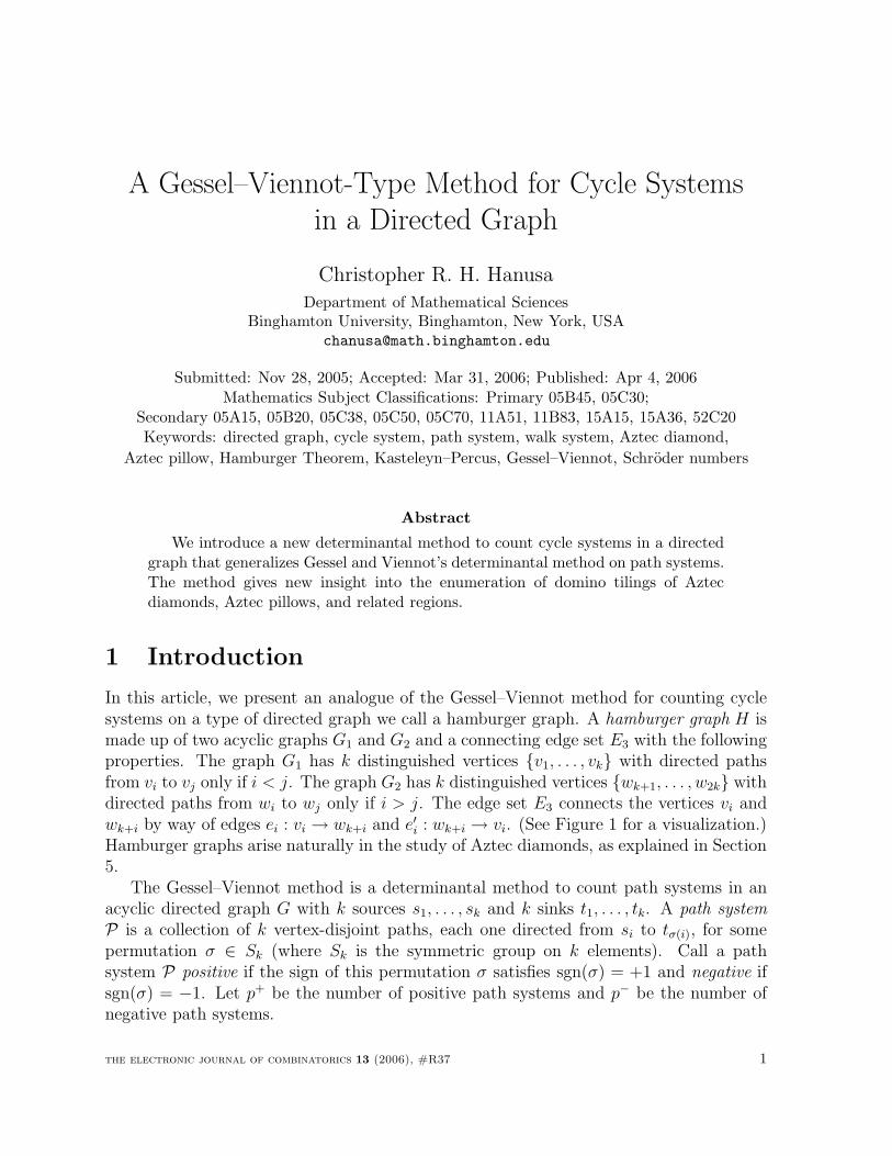
In this article, we present an analogue of the Gessel–Viennot method for counting cyclesystems on a type of directed graph we call a hamburger graph. A hamburger graph H ismade up of two acyclic graphs G1 and G2 and a connecting edge set E3 with the followingproperties. The graph G1 has k distinguished vertices {v1, . . . , vk} with directed pathsfrom vi to vj only if i < j. The graph G2 has k distinguished vertices {wk+1, . . . , w2k} withdirected paths from wi to wj only if i > j. The edge set E3 connects the vertices vi andwk+i by way of edges ei : vi → wk+i and e′i : wk+i → vi. (See Figure 1 for a visualization.)Hamburger graphs arise naturally in the study of Aztec diamonds, as explained in Section5.

The Gessel–Viennot method is a determinantal method to count path systems in anacyclic directed graph G with k sources s1, . . . , sk and k sinks t1, . . . , tk. A path systemP is a collection of k vertex-disjoint paths, each one directed from si to tσ(i), for somepermutation σ ∈ Sk (where Sk is the symmetric group on k elements). Call a pathsystem P positive if the sign of this permutation σ satisfies sgn(σ) = +1 and negative ifsgn(σ) = −1. Let p+ be the number of positive path systems and p− be the number ofnegative path systems.

the electronic journal of combinatorics 13 (2006), #R37 1

vk

wk+1 wk+2 w2k

G1

E3

G2

e′1 e1

v2v1

Figure 1: A hamburger graph

Corresponding to this graph G is a k× k matrix A = (aij), where aij is the number ofpaths from si to tj in G. The result of Gessel and Viennot states that det A = p+ − p−.The Gessel–Viennot method was introduced in [4, 5], and has its roots in works by Karlinand McGregor [8] and Lindstrom [10]. A nice exposition of the method and applicationsis given in the article by Aigner [1].

This article concerns a similar determinantal method for counting cycle systems in ahamburger graph H . A cycle system C is a collection of vertex-disjoint directed cycles inH . Let l be the number of edges in C that travel from G2 to G1 and let m be the numberof cycles in C. Call a cycle system positive if (−1)l+m = +1 and negative if (−1)l+m = −1.Let c+ be the number of positive cycle systems and c− be the number of negative cyclesystems. Corresponding to each hamburger graph H is a 2k× 2k block matrix MH of theform

MH =

[A Ik

−Ik B

],

where in the upper triangular matrix A = (aij), aij is the number of paths from vi to vj

in G1 and in the lower triangular matrix B = (bij), bij is the number of paths from wk+i

to wk+j in G2. This matrix MH is referred to as a hamburger matrix.

Theorem 1.1 (The Hamburger Theorem). If H is a hamburger graph, then det MH =c+ − c−.

A hamburger graph H is called strongly planar if there is a planar embedding of Hthat sends vi to (i, 1) and wk+i to (i,−1) for all 1 ≤ i ≤ k, and keeps edges of E1 in thehalf-space y ≥ 1 and edges of E2 in the half-space y ≤ −1. This definition suggests thatG1 and G2 are “relatively” planar in H , a stronger condition than planarity of H . Noticethat when H is strongly planar, each cycle must use exactly one edge from G2 to G1.Hence, the sign of every cycle system is +1. This implies the following corollary.

Corollary 1.2. If H is a strongly planar hamburger graph, det MH = c+.

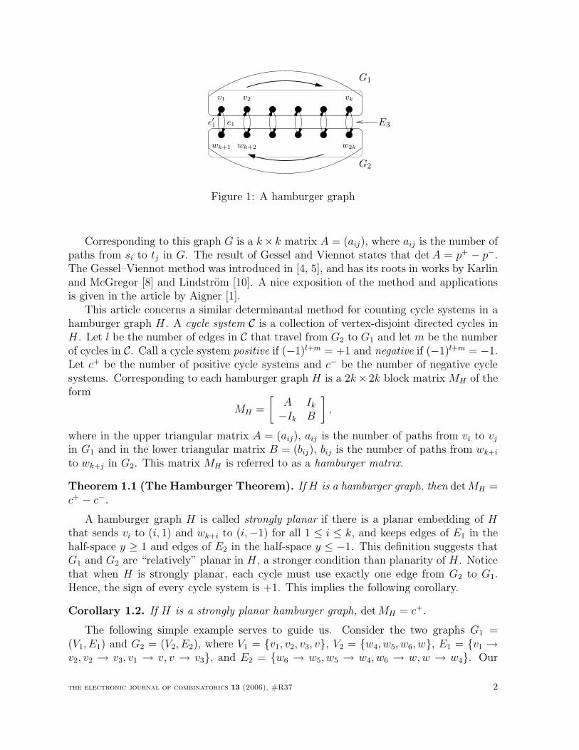
The following simple example serves to guide us. Consider the two graphs G1 =(V1, E1) and G2 = (V2, E2), where V1 = {v1, v2, v3, v}, V2 = {w4, w5, w6, w}, E1 = {v1 →v2, v2 → v3, v1 → v, v → v3}, and E2 = {w6 → w5, w5 → w4, w6 → w, w → w4}. Our


v∗

v1 v3

w4 w6

v2

w∗

w5

Figure 2: A simple hamburger graph H

hamburger graph H will be the union of G1, G2, and the edge set E3. In this example,k = 3 and H is strongly planar. Figure 2 gives a graphical representation of H .

In this example, the hamburger matrix MH equals

MH =

1 1 2 1 0 00 1 1 0 1 00 0 1 0 0 1−1 0 0 1 0 00 −1 0 1 1 00 0 −1 2 1 1

.

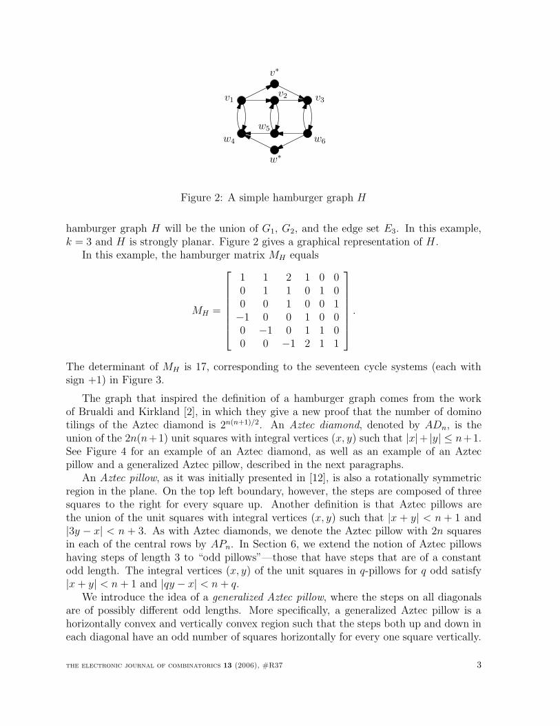
The determinant of MH is 17, corresponding to the seventeen cycle systems (each withsign +1) in Figure 3.

The graph that inspired the definition of a hamburger graph comes from the workof Brualdi and Kirkland [2], in which they give a new proof that the number of dominotilings of the Aztec diamond is 2n(n+1)/2. An Aztec diamond, denoted by ADn, is theunion of the 2n(n+1) unit squares with integral vertices (x, y) such that |x|+ |y| ≤ n+1.See Figure 4 for an example of an Aztec diamond, as well as an example of an Aztecpillow and a generalized Aztec pillow, described in the next paragraphs.

An Aztec pillow, as it was initially presented in [12], is also a rotationally symmetricregion in the plane. On the top left boundary, however, the steps are composed of threesquares to the right for every square up. Another definition is that Aztec pillows arethe union of the unit squares with integral vertices (x, y) such that |x + y| < n + 1 and|3y − x| < n + 3. As with Aztec diamonds, we denote the Aztec pillow with 2n squaresin each of the central rows by APn. In Section 6, we extend the notion of Aztec pillowshaving steps of length 3 to “odd pillows”—those that have steps that are of a constantodd length. The integral vertices (x, y) of the unit squares in q-pillows for q odd satisfy|x + y| < n + 1 and |qy − x| < n + q.

We introduce the idea of a generalized Aztec pillow, where the steps on all diagonalsare of possibly different odd lengths. More specifically, a generalized Aztec pillow is ahorizontally convex and vertically convex region such that the steps both up and down ineach diagonal have an odd number of squares horizontally for every one square vertically.


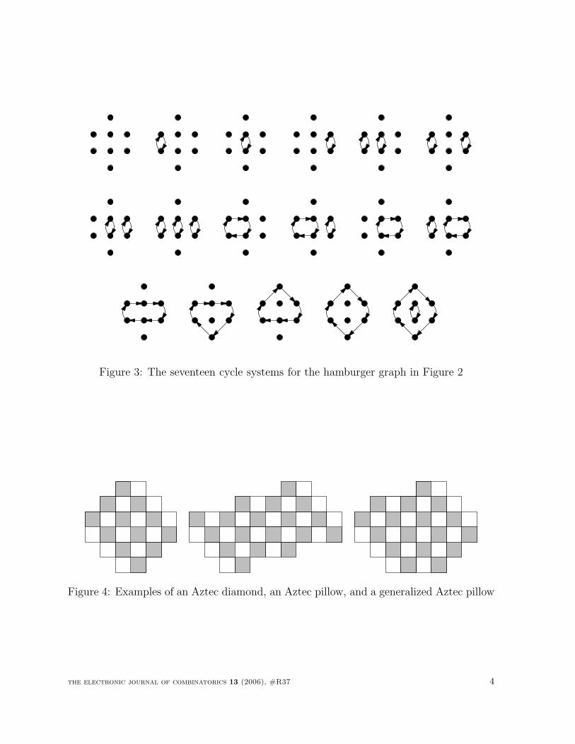
Figure 3: The seventeen cycle systems for the hamburger graph in Figure 2

Figure 4: Examples of an Aztec diamond, an Aztec pillow, and a generalized Aztec pillow


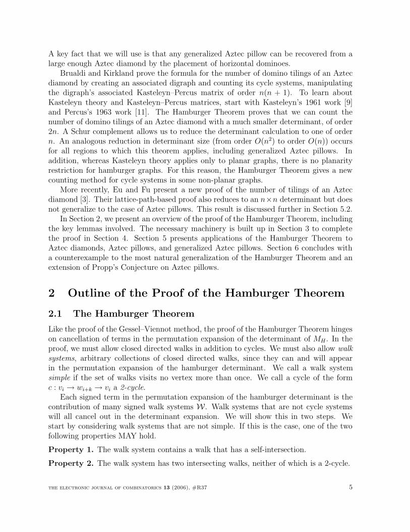
A key fact that we will use is that any generalized Aztec pillow can be recovered from alarge enough Aztec diamond by the placement of horizontal dominoes.

Brualdi and Kirkland prove the formula for the number of domino tilings of an Aztecdiamond by creating an associated digraph and counting its cycle systems, manipulatingthe digraph’s associated Kasteleyn–Percus matrix of order n(n + 1). To learn aboutKasteleyn theory and Kasteleyn–Percus matrices, start with Kasteleyn’s 1961 work [9]and Percus’s 1963 work [11]. The Hamburger Theorem proves that we can count thenumber of domino tilings of an Aztec diamond with a much smaller determinant, of order2n. A Schur complement allows us to reduce the determinant calculation to one of ordern. An analogous reduction in determinant size (from order O(n2) to order O(n)) occursfor all regions to which this theorem applies, including generalized Aztec pillows. Inaddition, whereas Kasteleyn theory applies only to planar graphs, there is no planarityrestriction for hamburger graphs. For this reason, the Hamburger Theorem gives a newcounting method for cycle systems in some non-planar graphs.

More recently, Eu and Fu present a new proof of the number of tilings of an Aztecdiamond [3]. Their lattice-path-based proof also reduces to an n×n determinant but doesnot generalize to the case of Aztec pillows. This result is discussed further in Section 5.2.

In Section 2, we present an overview of the proof of the Hamburger Theorem, includingthe key lemmas involved. The necessary machinery is built up in Section 3 to completethe proof in Section 4. Section 5 presents applications of the Hamburger Theorem toAztec diamonds, Aztec pillows, and generalized Aztec pillows. Section 6 concludes witha counterexample to the most natural generalization of the Hamburger Theorem and anextension of Propp’s Conjecture on Aztec pillows.

2 Outline of the Proof of the Hamburger Theorem

2.1 The Hamburger Theorem

Like the proof of the Gessel–Viennot method, the proof of the Hamburger Theorem hingeson cancellation of terms in the permutation expansion of the determinant of MH . In theproof, we must allow closed directed walks in addition to cycles. We must also allow walksystems, arbitrary collections of closed directed walks, since they can and will appearin the permutation expansion of the hamburger determinant. We call a walk systemsimple if the set of walks visits no vertex more than once. We call a cycle of the formc : vi → wi+k → vi a 2-cycle.

Each signed term in the permutation expansion of the hamburger determinant is thecontribution of many signed walk systems W. Walk systems that are not cycle systemswill all cancel out in the determinant expansion. We will show this in two steps. Westart by considering walk systems that are not simple. If this is the case, one of the twofollowing properties MAY hold.

Property 1. The walk system contains a walk that has a self-intersection.

Property 2. The walk system has two intersecting walks, neither of which is a 2-cycle.


The following lemma shows that the contributions of walk systems satisfying either ofthese two properties cancel in the permutation expansion of the determinant of MH .

Lemma 2.1. The set of all walk systems W that satisfy either Property 1 or Property2 can be partitioned into equivalence classes, each of which contributes a net zero to thepermutation expansion of the determinant of MH .

The proof of Lemma 2.1 uses a generalized involution principle. Walk systems cancelin families based on the their “first” intersection point.

The remainder of the cancellation in the determinant expansion is based on the conceptof a minimal walk system; we motivate this definition by asking the following questions.What kind of walk systems does the permutation expansion of the hamburger determinantgenerate, and how is this different from our original notion of cycle systems that we wantedto count in the introduction? The key difference is that the same collection of walks canbe generated by multiple terms in the determinantal expansion of MH ; whereas, we wouldonly want to count it once as a cycle system. This redundancy arises when the walk visitsthree distinguished vertices in G1 without passing via G2 or vice versa. We illustrate thisnotion with the following example.

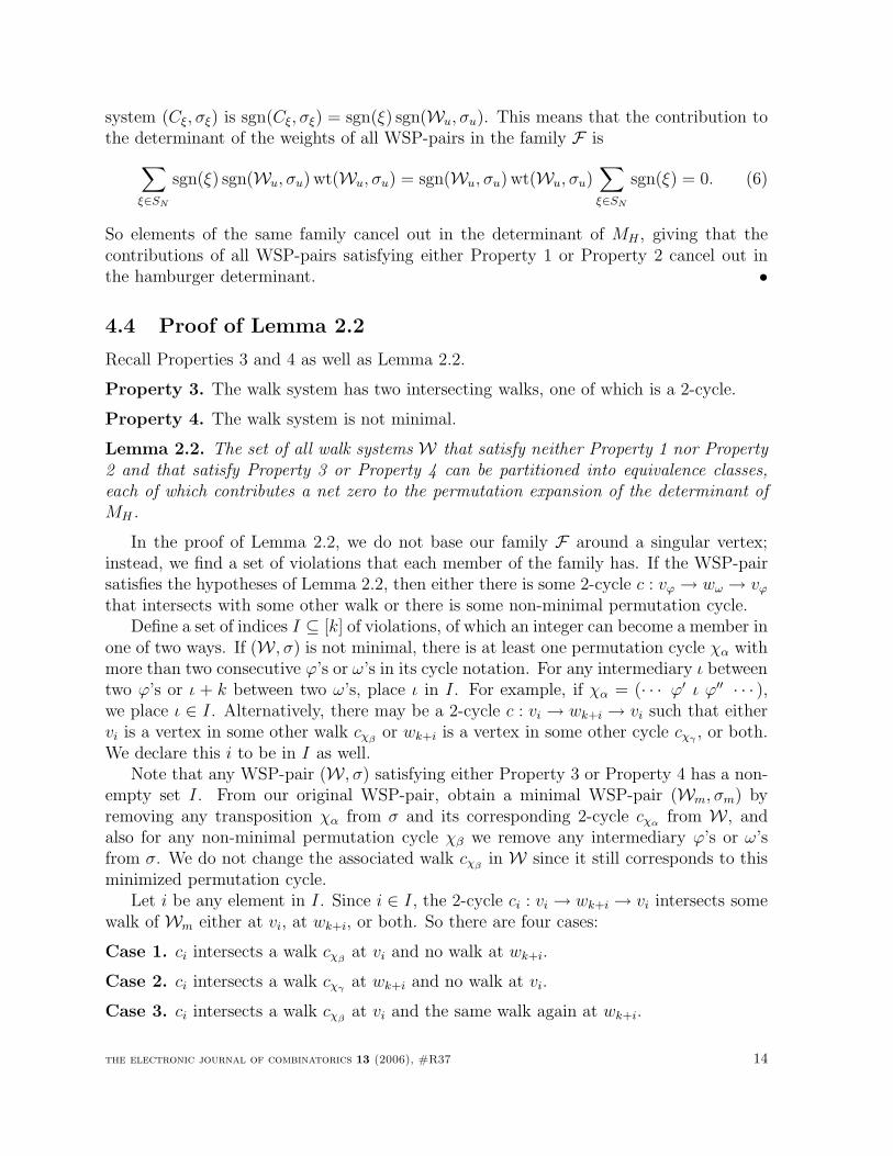
Consider the second cycle system in the third row of Figure 3, consisting of onesolitary directed cycle. Since this cycle visits vertices v1, v2, v3, w6, and w4 in thatorder, it contributes a non-zero weight in the permutation expansion of the determinantcorresponding to the term (12364) in S6. Notice that this cycle also contributes a non-zero weight in the permutation expansion of the determinant corresponding to the term(1364). We see this since our cycle follows a path from v1 to v3 (by way of v2), returningto v1 via w6 and w4. We must deal with this ambiguity. We introduce the idea of aminimal permutation cycle, one which does not include more than two successive entrieswith values between 1 and k or between k + 1 and 2k. We see that (1364) is minimalwhile (12364) is not.

We notice that walk systems arise from permutations, so it is natural to think ofa walk system as a permutation together with a collection of walks that “follow” thepermutation. This is the idea of a walk system–permutation pair (or WSP-pair for short)that is presented in Section 3.4. From the idea of a minimal permutation cycle, we definea minimal walk to have as its base permutation a minimal permutation cycle, and aminimal walk system to be composed of only minimal walks. Since our original goal wasto count “cycle systems” in a directed graph, we realize we need to be precise and insteadcount “simple minimal walk systems”. This leads to the second part of the proof of theHamburger Theorem.

Given a walk system that is either not simple or not minimal and that satisfies neitherProperty 1 nor Property 2, at least one of the two following properties MUST hold.

Property 3. The walk system has two intersecting walks, one of which is a 2-cycle.

Property 4. The walk system is not minimal.

The following lemma shows that the contributions of walk systems satisfying either ofthese new properties cancel in the permutation expansion of the determinant of MH .


Lemma 2.2. The set of all walk systems W that satisfy neither Property 1 nor Property2 and that satisfy Property 3 or Property 4 can be partitioned into equivalence classes,each of which contributes a net zero to the permutation expansion of the determinant ofMH .

The proof of Lemma 2.2 is also based on involutions. Walk systems cancel in familiesbuilt from an index set containing the set of all 2-cycle intersections and non-minimalities.

If a walk system satisfies none of the conditions of Properties 1 through 4, then it isindeed a simple minimal walk system, or in other words, a cycle system. The cancellationfrom the above sets of families gives that only cycle systems contribute to the permutationexpansion of the determinant of MH . This contribution is the signed weight of each cyclesystem, so the determinant of MH exactly equals c+ − c−. Theorem 1.1 follows fromLemmas 2.1 and 2.2 in Section 4. •

2.2 The Weighted Hamburger Theorem

There is also a weighted version of the Hamburger Theorem, and it will be under thisgeneralization that Lemmas 2.1 and 2.2 are proved. We allow weights wt(e) on the edges ofthe hamburger graph; the simplest weighting, which counts the number of cycle systems,assigns wt(e) ≡ 1. We require that wt(ei)wt(e′i) = 1 for all 2 ≤ i ≤ k − 1, but we donot require this condition for i = 1 nor for i = k. Define the 2k × 2k weighted hamburgermatrix MH to be the block matrix

MH =

[A D1

−D2 B

]. (1)

In the upper-triangular k × k matrix A = (aij), aij is the sum of the products of theweights of edges over all paths from vi to vj in G1. In the lower triangular k × k matrixB = (bij), bij is the sum of the products of the weights of edges over all paths from wk+i towk+j in G2. The diagonal k× k matrix D1 has as its entries dii = wt(ei) and the diagonalk × k matrix D2 has as its entries dii = wt(e′i). Note that when the weights of the edgesin E3 are all 1, these matrices satisfy D1 = D2 = Ik.

We wish to count vertex-disjoint unions of weighted cycles in H . In any hamburgergraph H , there are two possible types of cycle. There are k 2-cycles

c : viei−→ wk+i

e′i−→ vi

and many more general cycles that alternate between G1 and G2. We can think of ageneral cycle as a path P1 in G1 connected by an edge e1,1 ∈ E3 to a path Q1 in G2,which in turn connects to a path P2 in G1 by an edge e′1,2, continuing in this fashion untilarriving at a final path Ql in G2 whose terminal vertex is adjacent to the initial vertex ofP1. We write

c : P1e1,1−→ Q1

e′1,2−→ P2e2,1−→ · · · el,1−→ Pl

e′l,2−→ Ql.


For each cycle c, we define the weight wt(c) of c to be the product of the weights of alledges traversed by c:

wt(c) =∏e∈c

wt(e).

We define a weighted cycle system to be a collection C of m vertex-disjoint cycles. Weagain define the sign of a weighted cycle system to be sgn(C) = (−1)l+m, where l is thetotal number of edges from G2 to G1 in C. We say that a weighted cycle system C ispositive if sgn(C) = +1 and negative if sgn(C) = −1. For a hamburger graph H , let c+ bethe sum of the weights of positive weighted cycle systems, and let c− be the sum of theweights of negative weighted cycle systems.

Theorem 2.3 (The weighted Hamburger Theorem). The determinant of the weigh-ted hamburger matrix MH equals c+ − c−.

As above, Theorem 2.3 follows from Lemmas 2.1 and 2.2. The proofs will be presentedafter developing the following necessary machinery.

3 Additional Definitions

3.1 Edge Cycles and Permutation Cycles

In the proof of the Hamburger Theorem, there are two distinct mathematical objects thathave the name “cycle”. We have already mentioned the type of cycle that appears ingraph theory. There, a (simple) cycle in a directed graph is a closed directed path withno repeated vertices.

Secondly, there is a notion of cycle when we talk about permutations. If σ ∈ Sn is apermutation, we can write σ as the product of disjoint cycles σ = χ1χ2 · · ·χτ .

To distinguish between these two types of cycles when confusion is possible, we call theformer kind an edge cycle and the latter kind a permutation cycle. Notationally, we useRoman letters when discussing edge cycles and Greek letters when discussing permutationcycles.

3.2 Permutation Expansion of the Determinant

We recall that the permutation expansion of the determinant of an n×n matrix M = (mij)is the expansion of the determinant as

det M =∑σ∈Sn

(sgn σ)m1,σ(1) · · ·mn,σ(n). (2)

We will be considering non-zero terms in the permutation expansion of the determinantof the hamburger matrix MH . Because of the special block form of the hamburger matrixin Equation (1), the permutations σ that make non-zero contributions to this sum areproducts of disjoint cycles of either of two forms—the simple transposition

χ = (ϕ11 ω11)


or the general permutation cycle

χ = (ϕ11 ϕ12 · · · ϕ1µ1 ω11 ω12 · · · ω1ν1 ϕ21 · · · · · · ϕλµλωλ1 · · · ωλνλ

). (3)

In the first case, ω11 = ϕ11 + k. In the second case, 1 ≤ ϕικ ≤ k, k + 1 ≤ ωικ ≤ 2k,ϕικ < ϕι,κ+1, and ωικ > ωι,κ+1 for all 1 ≤ ι ≤ λ and relevant κ. The block matrix form alsoimplies that ϕιµι +k = ωι1, ωινι −k = ϕι+1,1, and ωλνλ

−k = ϕ11. These last requirementsalong with the fact that no integers appear more than once in a permutation cycle implythat µi, νi ≥ 2 for 1 ≤ i ≤ λ. So that this permutation cycle is in standard form, we makesure that ϕ11 = minι,κ ϕικ. In order to refer to this value later, we define a function Φ byΦ(χ) = ϕ11. Each value 1 ≤ ϕι ≤ k or k + 1 ≤ ωι ≤ 2k appears at most once for anyσ ∈ S2k.

We call a permutation cycle χ minimal if it is a transposition or if µι = νι = 2 for allι. Minimality implies that we can write our general permutation cycles χ in the form

χ = (ϕ11 ϕ12 ω11 ω12 ϕ21 · · · ϕλ2 ωλ1 ωλ2), (4)

with the same conditions as before. We call a permutation σ = χ1 · · ·χτ minimal if eachof its cycles χι is minimal.

3.3 Walks Associated to a Permutation

To each permutation cycle χ ∈ S2k, we can associate one or more walks cχ in H .If χ is the transposition χ = (ϕ11 ω11), then we associate the 2-cycle cχ : vϕ11 →

wω11 → vϕ11 to χ. To any permutation cycle χ that is not a transposition, we canassociate multiple walks cχ by gluing together paths that follow χ in the following way.If χ has the form of Equation (3), then for each 1 ≤ i ≤ λ, let Pi be any path in G1 thatvisits each of the vertices vϕi1

, vϕi2, all the way through vϕiµi

in order. Similarly, let Qi

be any path in G2 that visits each of the vertices wωi1, wωi2

, through wωiνiin order. For

each choice of paths Pi and Qi, we have a possibility for the walk cχ; we can set

cχ : P1

eϕ12−→ Q1

e′ϕ21−→ P2

eϕ22−→ · · · · · · e′ϕλ1−→ Pλ

eϕλ2−→ Qλ. (5)

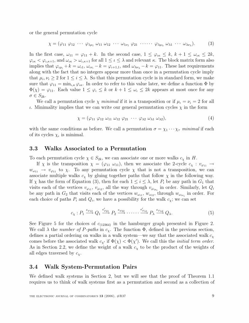
See Figure 5 for the choices of c(12364) in the hamburger graph presented in Figure 2.We call λ the number of P -paths in cχ. The function Φ, defined in the previous section,defines a partial ordering on walks in a walk system—we say that the associated walk cχ

comes before the associated walk cχ′ if Φ(χ) < Φ(χ′). We call this the initial term order.As in Section 2.2, we define the weight of a walk cχ to be the product of the weights ofall edges traversed by cχ.

3.4 Walk System-Permutation Pairs

We defined walk systems in Section 2, but we will see that the proof of Theorem 1.1requires us to think of walk systems first as a permutation and second as a collection of


orχ = (1 2 3 6 4 )

Figure 5: A permutation cycle χ and the two walks in H associated to χ

walks determined by the permutation. We will see that for cycle systems as presentedinitially, signs and weights are not changed by this recharacterization.

If H is a hamburger graph with k pairs of distinguished vertices, we define a walksystem–permutation pair as follows.

Definition 3.1. A walk system–permutation pair (or WSP-pair for short) is a pair (W, σ),where σ ∈ S2k is a permutation and W is a collection of walks c ∈ W with the followingproperty: if the disjoint cycle representation of σ is σ = χ1 · · ·χτ , then W is a collectionof τ walks cχι , for 1 ≤ ι ≤ τ , where cχι is a walk associated to the permutation cycle χι.

We define the weight of a WSP-pair (W, σ) to be the product of the weights of theassociated walks cχ ∈ W.

Each permutation σ yields many collections of walks W, collections of walks W maybe associated to many permutations σ, but any walk system W corresponds to one andonly one minimal permutation σm. This is because, given any path as in Equation (5),we can read off the initial and terminal vertices of each Pi and Qi in order, producing awell-defined permutation cycle σm. We define a WSP-pair (W, σ) to be minimal if σ is aminimal permutation.

For a WSP-pair (W, σ), where σ = χ1 · · ·χτ , we define the sign of the WSP-pair,sgn(W, σ), to be (−1)lsgn(σ), where λχ is the number of P -paths in cχ and where l =∑

cχ∈W λχ. Alternatively, we could consider the sign of (W, σ) to be the product of the

signs of its associated walks cχ, where the sign of cχ is sgn(cχ) = (−1)λχsgn(χ). We saythat a WSP-pair (W, σ) is positive if sgn(W, σ) = +1 and is negative if sgn(W, σ) = −1.

Note that if (W, σ) is a minimal WSP-pair, then sgn(cχ) = +1 for a transposition χand sgn(cχ) = (−1)λ+1 if χ is of the form in Equation (4). In particular, when (W, σ)is minimal and simple, its sign and weight is consistent with the definition given in theintroduction.


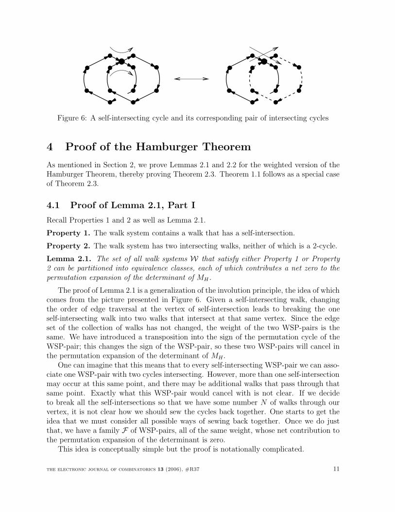
Figure 6: A self-intersecting cycle and its corresponding pair of intersecting cycles

4 Proof of the Hamburger Theorem

As mentioned in Section 2, we prove Lemmas 2.1 and 2.2 for the weighted version of theHamburger Theorem, thereby proving Theorem 2.3. Theorem 1.1 follows as a special caseof Theorem 2.3.

4.1 Proof of Lemma 2.1, Part I

Recall Properties 1 and 2 as well as Lemma 2.1.

Property 1. The walk system contains a walk that has a self-intersection.

Property 2. The walk system has two intersecting walks, neither of which is a 2-cycle.

Lemma 2.1. The set of all walk systems W that satisfy either Property 1 or Property2 can be partitioned into equivalence classes, each of which contributes a net zero to thepermutation expansion of the determinant of MH .

The proof of Lemma 2.1 is a generalization of the involution principle, the idea of whichcomes from the picture presented in Figure 6. Given a self-intersecting walk, changingthe order of edge traversal at the vertex of self-intersection leads to breaking the oneself-intersecting walk into two walks that intersect at that same vertex. Since the edgeset of the collection of walks has not changed, the weight of the two WSP-pairs is thesame. We have introduced a transposition into the sign of the permutation cycle of theWSP-pair; this changes the sign of the WSP-pair, so these two WSP-pairs will cancel inthe permutation expansion of the determinant of MH .

One can imagine that this means that to every self-intersecting WSP-pair we can asso-ciate one WSP-pair with two cycles intersecting. However, more than one self-intersectionmay occur at this same point, and there may be additional walks that pass through thatsame point. Exactly what this WSP-pair would cancel with is not clear. If we decideto break all the self-intersections so that we have some number N of walks through ourvertex, it is not clear how we should sew the cycles back together. One starts to get theidea that we must consider all possible ways of sewing back together. Once we do justthat, we have a family F of WSP-pairs, all of the same weight, whose net contribution tothe permutation expansion of the determinant is zero.

This idea is conceptually simple but the proof is notationally complicated.


If W satisfies either Property 1 or Property 2, then there is some vertex of intersection,be it either a self-intersection or an intersection of two walks. Our aim is to choose a well-defined first point of intersection at which we will build the family F . The initial termorder gives an order on walks associated to permutation cycles; we choose the earliestwalk cχα that has some vertex of intersection. Once we have determined the earliest walk,we start at vΦ(cχα ) and follow the walk

cχa : P1 → Q1 → P2 → · · · → Pm → Qm,

until we reach a vertex of intersection.In our discussion, we make the assumption that this first vertex of intersection is a

vertex v∗ in G1. A similar argument exists if the first appearance occurs in G2. Noticethat at v∗ there may be multiple self-intersections or multiple intersections of walks. Wewill create a family F of WSP-pairs that takes into account each of these possibilities.

If we want to rigorously define the breaking of a self-intersecting walk at a vertex ofself-intersection, we need to specify many different components of the WSP-pair (C, σ).First, we need to specify on which walk in W we are acting. Next, we need to specify thevertex of self-intersection. Since this self-intersection vertex may occur in multiple paths,we need to specify which two paths we interchange in the breaking process.

4.2 Definitions of Breaking and Sewing

In the following paragraphs, we define “breaking” on WSP-pairs, which takes in a WSP-pair (W, σ), one of σ’s permutation cycles χα, the associated walk cχα, paths Py and Pz incχα, and the vertex v∗ in both Py and Pz where cχα has a self-intersection. For simplicity,we assume that v∗ is not a distinguished vertex, but the argument still holds in that case.The inverse of this operation is “sewing”.

In this framework, cχα has the form

cχα : P1 → Q1 → P2 → · · · → Py → Qy → · · · → Pz → Qz → · · · → Pl → Ql,

where the paths Py and Pz in G1 are separated into two halves as

Py : P (1)y → v∗ → P (2)

y

andPz : P (1)

z → v∗ → P (2)z .

Remember that Py and Pz are paths that stop over at various vertices depending onthe permutation χα. The vertex v∗ must have adjacent stop-over vertices in each of thetwo paths Py and Pz. Let the nearest stop-over vertices on the paths Py and Pz be vϕy

and vϕy+1, and vϕz and vϕz+1, respectively.This implies χα has the form

χα = (ϕ11 · · · ϕ1µ1 ω11 · · · ϕy ϕy+1 · · · ϕz ϕz+1 · · · ϕλµλωλ1 · · · ωλνλ

).


We can now precisely define the result of breaking. We define χβ and χγ by splittingχα as follows:

χβ = (ϕ11 · · · ϕy ϕz+1 · · · ωλνλ)

andχγ = (ϕy+1 · · · ϕz),

with the necessary rewriting of χγ to have as its initial entry the value Φ(χγ). Define cχβ

and cχγ to be

cχβ: P1 → Q1 → P2 → · · · → P (1)

y → v∗ → P (2)z → Qz → · · · → Pl → Ql,

andcχγ : P (1)

z → v∗ → P (2)y → Qy → · · · → Qz−1,

again changing the starting vertex of cχγ to vΦ(cχγ ).We define the breaking of the WSP-pair with the above inputs to be the WSP-pair

(W ′, σ′) such thatW ′ = W ∪ {cχβ

, cχγ} \ {cχα}and

σ′ = σχ−1α χβχγ = σ · (ϕy+1 ϕz+1).

The edge set of W is equal to the edge set of W ′, so the weight of the modified cyclesystems is the same as the original. Since we changed σ to σ′ by multiplying only by atransposition, the sign of the modified WSP-pair is opposite to that of the original.

By only discussing the case when v∗ is not distinguished, we avoid notational issuesbrought upon by cases when v∗ is or is not one of the stop-over vertices.

4.3 Proof of Lemma 2.1, Part II

Having defined breaking and sewing, we can continue the proof.For any WSP-pair (W, σ) satisfying either Property 1 or Property 2, let cχα ∈ W be

the first walk in the initial term order with an vertex of intersection. Let v∗ be the firstvertex of intersection in cχα . Then for all walks c with one or more self-intersections at v∗,continue to break c at v∗ until there are no more self-intersections. Define the resultingWSP-pair (Wu, σu) to be the unlinked WSP-pair associated to (W, σ). In (Wu, σu), thereis some number N of general walks intersecting at vertex v∗. There may be a 2-cycleintersecting v∗ as well, but this does not matter.

For any permutation ξ ∈ SN , let ξ = ζ1ζ2 · · · ζη be its cycle representation, where eachζι is a cycle. For each 1 ≤ ι ≤ η, sew together walks in order: if ζι = (δι1 · · · διει), sewtogether cχδι1

and cχδι2at v∗. Sew this result together with cχδι3

, and so on through cχδιει.

Note that the result of these sewings is unique, and that every WSP-pair (W, σ) with(Wu, σu) as its unlinked WSP-pair can be obtained in this way, and no other WSP-pairappears. We can perform this procedure for any ξ ∈ SN ; the sign of the resulting walk


system (Cξ, σξ) is sgn(Cξ, σξ) = sgn(ξ) sgn(Wu, σu). This means that the contribution tothe determinant of the weights of all WSP-pairs in the family F is∑

ξ∈SN

sgn(ξ) sgn(Wu, σu) wt(Wu, σu) = sgn(Wu, σu) wt(Wu, σu)∑ξ∈SN

sgn(ξ) = 0. (6)

So elements of the same family cancel out in the determinant of MH , giving that thecontributions of all WSP-pairs satisfying either Property 1 or Property 2 cancel out inthe hamburger determinant. •

4.4 Proof of Lemma 2.2

Recall Properties 3 and 4 as well as Lemma 2.2.

Property 3. The walk system has two intersecting walks, one of which is a 2-cycle.

Property 4. The walk system is not minimal.

Lemma 2.2. The set of all walk systems W that satisfy neither Property 1 nor Property2 and that satisfy Property 3 or Property 4 can be partitioned into equivalence classes,each of which contributes a net zero to the permutation expansion of the determinant ofMH .

In the proof of Lemma 2.2, we do not base our family F around a singular vertex;instead, we find a set of violations that each member of the family has. If the WSP-pairsatisfies the hypotheses of Lemma 2.2, then either there is some 2-cycle c : vϕ → wω → vϕ

that intersects with some other walk or there is some non-minimal permutation cycle.Define a set of indices I ⊆ [k] of violations, of which an integer can become a member in

one of two ways. If (W, σ) is not minimal, there is at least one permutation cycle χα withmore than two consecutive ϕ’s or ω’s in its cycle notation. For any intermediary ι betweentwo ϕ’s or ι + k between two ω’s, place ι in I. For example, if χα = (· · · ϕ′ ι ϕ′′ · · · ),we place ι ∈ I. Alternatively, there may be a 2-cycle c : vi → wk+i → vi such that eithervi is a vertex in some other walk cχβ

or wk+i is a vertex in some other cycle cχγ , or both.We declare this i to be in I as well.

Note that any WSP-pair (W, σ) satisfying either Property 3 or Property 4 has a non-empty set I. From our original WSP-pair, obtain a minimal WSP-pair (Wm, σm) byremoving any transposition χα from σ and its corresponding 2-cycle cχα from W, andalso for any non-minimal permutation cycle χβ we remove any intermediary ϕ’s or ω’sfrom σ. We do not change the associated walk cχβ

in W since it still corresponds to thisminimized permutation cycle.

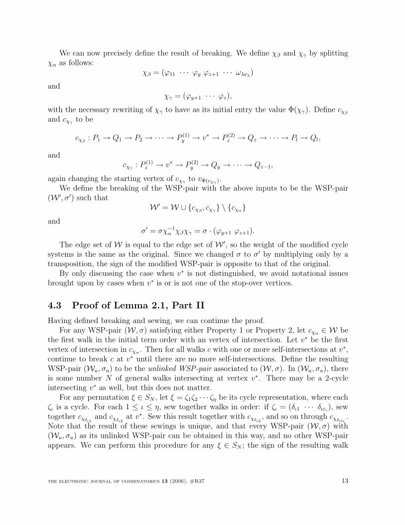
Let i be any element in I. Since i ∈ I, the 2-cycle ci : vi → wk+i → vi intersects somewalk of Wm either at vi, at wk+i, or both. So there are four cases:

Case 1. ci intersects a walk cχβat vi and no walk at wk+i.

Case 2. ci intersects a walk cχγ at wk+i and no walk at vi.

Case 3. ci intersects a walk cχβat vi and the same walk again at wk+i.


3)

1) 2)

4)

Figure 7: The four cases in which a walk can intersect with a 2-cycle

Case 4. ci intersects a walk cχβat vi and another walk cχγ at wk+i.

See Figure 7 for a picture.In order to build the family F , we modify the minimal WSP-pair (Wm, σm) at each

i with some choice of options, each giving a possible WSP-pair that has (Wm, σm) as itsminimal WSP-pair. We define a set of two or four options Oi for each i.

In Case 1, there are two options. Let o1 be the option of including the walk ci inWm and its corresponding transposition χα in σm. Let o2 be the option of including theintermediary ϕ = i in χβ in the position where cχβ

passes through vi.[Note that we could not apply both options at the same time since the resulting χα

and χβ would not be disjoint and therefore is not a term in the permutation expansion ofthe determinant.]

Similarly in Case 2, there are two options. Let o1 be the option of including the walkci in Wm and its corresponding transposition χα in σm. Let o2 be the option of includingthe intermediary ω = i + k in χγ in the position where cχγ passes through wk+i.

In Case 3, there are four options. Let o1 be the option of including the walk ci inWm and its corresponding transposition χα in σm. Let o2 be the option of including theintermediary ϕ = i in χβ in the position where cχβ

passes through vi. Let o3 be the optionof including the intermediary ω = i + k in χβ in the position where cχβ

passes throughwk+i. Let o4 be the option of including both intermediaries ϕ = i and ω = i + k in χβ inthe respective positions where cχβ

passes through vi and wk+i.In Case 4, there are four options. Let o1 be the option of including the walk ci in

Wm and its corresponding transposition χα in σm. Let o2 be the option of including theintermediary ϕ = i in χβ in the position where cχβ

passes through vi. Let o3 be the optionof including the intermediary ω = i + k in χγ in the position where cχγ passes throughwk+i. Let o4 be the option of including intermediary ϕ = i in χβ in the position where


sign = +1(1364)(25) (12364)

sign = −1

Figure 8: A family of two walk systems that cancel in the hamburger determinant

cχβpasses through vi and intermediary ω = i + k in χγ in the position where cχγ passes

through wk+i.

Corresponding to the associated minimal WSP-pair (Wm, σm) and index set I, definethe family F to be the set of WSP-pairs (Wf , σf ) by exercising all combinations of optionsoji

∈ Oi on (Wm, σm) for each i ∈ I. Note that every WSP-pair derived in this fashion is aWSP-pair satisfying the hypotheses of Lemma 2.2 and is such that its associated minimalWSP-pair is (Wm, σm). There is also no other WSP-pair (W ′, σ′) with (Wm, σm) as itsminimal WSP-pair. See Figure 8 for a canceling family of two walk systems, one of whichis the non-minimal walk system from Figure 5.

Every WSP-pair in F has the same weight since each option changes the edge setof W by at most a 2-cycle vi → wk+i → vi, where 2 ≤ i ≤ k − 1 and each of those2-cycles contributes a multiplier of 1 to the weight of the WSP-pair. The peculiar boundsin this restriction are due to the structure of the hamburger graph. A walk through thevertices v1 and wk+1 (or vk and w2k) must use edge e′1 (or ek), and include in its associatedpermutation cycle 1 and k + 1 (or k and 2k). This implies that we can not have multiplewalks through any of these four special vertices, as that would yield two non-disjointpermutation cycles in σ.

The sign of every WSP-pair in F is determined by the set of options applied to(Wm, σm). Each option oj contributes a multiplicative ±1 depending on j—sgn(o1) = +1,sgn(o2) = −1, and sgn(o3) = −1 and sgn(o4) = +1 if they exist.

Each family F contributes a cumulative weight of 0. This is because there are the samenumber of positive (Wf , σf ) ∈ F as negative (Wf , σf ) ∈ F . We see this since if i∗ ∈ I thenany set of WSP-pairs that exercise the same options oji

for all i 6= i∗ has either two or fourmembers (depending on the case of i∗), which split evenly between positive and negativeWSP-pairs. Since each family contributes a net zero to the hamburger determinant, thetotal contribution from WSP-pairs satisfying the hypotheses of Lemma 2.2 is zero. •

Since every WSP-pair appears once in the permutation expansion of det MH , the onlyWSP-pairs that contribute to the sum are those that are simple and minimal. Thereforedet MH is the sum over such WSP-pairs of sgn(W, σ)·wt(W, σ). This establishes Theorem2.3 and gives Theorem 1.1 as a special case.


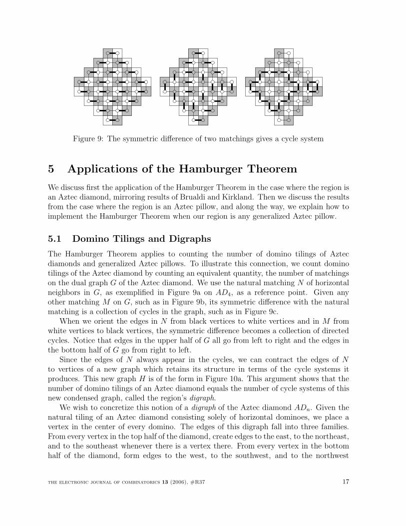
Figure 9: The symmetric difference of two matchings gives a cycle system

5 Applications of the Hamburger Theorem

We discuss first the application of the Hamburger Theorem in the case where the region isan Aztec diamond, mirroring results of Brualdi and Kirkland. Then we discuss the resultsfrom the case where the region is an Aztec pillow, and along the way, we explain how toimplement the Hamburger Theorem when our region is any generalized Aztec pillow.

5.1 Domino Tilings and Digraphs

The Hamburger Theorem applies to counting the number of domino tilings of Aztecdiamonds and generalized Aztec pillows. To illustrate this connection, we count dominotilings of the Aztec diamond by counting an equivalent quantity, the number of matchingson the dual graph G of the Aztec diamond. We use the natural matching N of horizontalneighbors in G, as exemplified in Figure 9a on AD4, as a reference point. Given anyother matching M on G, such as in Figure 9b, its symmetric difference with the naturalmatching is a collection of cycles in the graph, such as in Figure 9c.

When we orient the edges in N from black vertices to white vertices and in M fromwhite vertices to black vertices, the symmetric difference becomes a collection of directedcycles. Notice that edges in the upper half of G all go from left to right and the edges inthe bottom half of G go from right to left.

Since the edges of N always appear in the cycles, we can contract the edges of Nto vertices of a new graph which retains its structure in terms of the cycle systems itproduces. This new graph H is of the form in Figure 10a. This argument shows that thenumber of domino tilings of an Aztec diamond equals the number of cycle systems of thisnew condensed graph, called the region’s digraph.

We wish to concretize this notion of a digraph of the Aztec diamond ADn. Given thenatural tiling of an Aztec diamond consisting solely of horizontal dominoes, we place avertex in the center of every domino. The edges of this digraph fall into three families.From every vertex in the top half of the diamond, create edges to the east, to the northeast,and to the southeast whenever there is a vertex there. From every vertex in the bottomhalf of the diamond, form edges to the west, to the southwest, and to the northwest


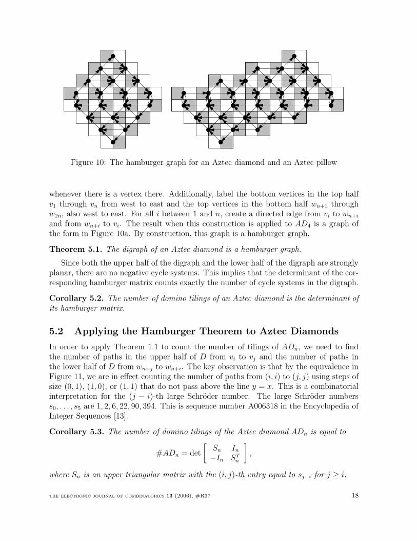
Figure 10: The hamburger graph for an Aztec diamond and an Aztec pillow

whenever there is a vertex there. Additionally, label the bottom vertices in the top halfv1 through vn from west to east and the top vertices in the bottom half wn+1 throughw2n, also west to east. For all i between 1 and n, create a directed edge from vi to wn+i

and from wn+i to vi. The result when this construction is applied to AD4 is a graph ofthe form in Figure 10a. By construction, this graph is a hamburger graph.

Theorem 5.1. The digraph of an Aztec diamond is a hamburger graph.

Since both the upper half of the digraph and the lower half of the digraph are stronglyplanar, there are no negative cycle systems. This implies that the determinant of the cor-responding hamburger matrix counts exactly the number of cycle systems in the digraph.

Corollary 5.2. The number of domino tilings of an Aztec diamond is the determinant ofits hamburger matrix.

5.2 Applying the Hamburger Theorem to Aztec Diamonds

In order to apply Theorem 1.1 to count the number of tilings of ADn, we need to findthe number of paths in the upper half of D from vi to vj and the number of paths inthe lower half of D from wn+j to wn+i. The key observation is that by the equivalence inFigure 11, we are in effect counting the number of paths from (i, i) to (j, j) using steps ofsize (0, 1), (1, 0), or (1, 1) that do not pass above the line y = x. This is a combinatorialinterpretation for the (j − i)-th large Schroder number. The large Schroder numberss0, . . . , s5 are 1, 2, 6, 22, 90, 394. This is sequence number A006318 in the Encyclopedia ofInteger Sequences [13].

Corollary 5.3. The number of domino tilings of the Aztec diamond ADn is equal to

#ADn = det

[Sn In

−In STn

],

where Sn is an upper triangular matrix with the (i, j)-th entry equal to sj−i for j ≥ i.


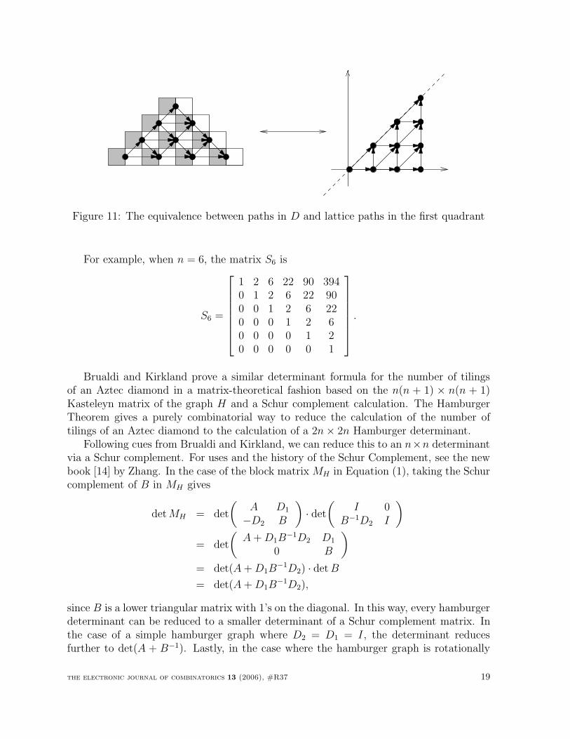
Figure 11: The equivalence between paths in D and lattice paths in the first quadrant

For example, when n = 6, the matrix S6 is

S6 =

1 2 6 22 90 3940 1 2 6 22 900 0 1 2 6 220 0 0 1 2 60 0 0 0 1 20 0 0 0 0 1

.

Brualdi and Kirkland prove a similar determinant formula for the number of tilingsof an Aztec diamond in a matrix-theoretical fashion based on the n(n + 1) × n(n + 1)Kasteleyn matrix of the graph H and a Schur complement calculation. The HamburgerTheorem gives a purely combinatorial way to reduce the calculation of the number oftilings of an Aztec diamond to the calculation of a 2n × 2n Hamburger determinant.

Following cues from Brualdi and Kirkland, we can reduce this to an n×n determinantvia a Schur complement. For uses and the history of the Schur Complement, see the newbook [14] by Zhang. In the case of the block matrix MH in Equation (1), taking the Schurcomplement of B in MH gives

det MH = det

(A D1

−D2 B

)· det

(I 0

B−1D2 I

)= det

(A + D1B

−1D2 D1

0 B

)= det(A + D1B

−1D2) · det B

= det(A + D1B−1D2),

since B is a lower triangular matrix with 1’s on the diagonal. In this way, every hamburgerdeterminant can be reduced to a smaller determinant of a Schur complement matrix. Inthe case of a simple hamburger graph where D2 = D1 = I, the determinant reducesfurther to det(A + B−1). Lastly, in the case where the hamburger graph is rotationally


symmetric, B = JAJ where J is the exchange matrix, which consists of 1’s down themain skew-diagonal and 0’s elsewhere. This implies that we can write the determinant interms of just the submatrix A, i.e., det(A + JA−1J). (Note that J−1 = J .)

Corollary 5.4. The number of domino tilings of the Aztec diamond ADn is equal todet(Sn + JnS

−1n Jn), where Jn is the n × n exchange matrix.

In the case of a hamburger graph H , we call this Schur complement, A+B−1, a reducedhamburger matrix. In the Aztec diamond graph example above, we can thus calculate thenumber of tilings of the Aztec diamond AD6 as follows. The inverse of S6 is

S−16 =

1 −2 −2 −6 −22 −900 1 −2 −2 −6 −220 0 1 −2 −2 −60 0 0 1 −2 −20 0 0 0 1 −20 0 0 0 0 1

,

which implies that the determinant of the reduced hamburger matrix

M6 =

2 2 6 22 90 394−2 2 2 6 22 90−2 −2 2 2 6 22−6 −2 −2 2 2 6−22 −6 −2 −2 2 2−90 −22 −6 −2 −2 2

gives the number of tilings of AD6.

Brualdi and Kirkland were the first to find such a determinantal formula for the numberof tilings of an Aztec diamond [2]. Their matrix was different only in the fact that eachentry was multiplied by (−1) and there was a multiplicative factor of (−1)n. Brualdi andKirkland were able to calculate the sequence of determinants, {det Mn}, using a J-fractionexpansion, which only works when matrices are Toeplitz or Hankel.

Eu and Fu also found an n × n determinant that calculated the number of tilings ofan Aztec diamond [3]. Their matrix also involves large Schroder numbers; when n = 6,their matrix is

1 2 6 22 90 3942 6 22 90 394 18066 22 90 394 1806 8558

22 90 394 1806 8558 4158690 394 1806 8558 41586 206098

394 1806 8558 41586 206098 1037718

.

Their proof hinges on the relationship between domino tilings in an Aztec diamond andpath systems in a lattice derived from the Aztec diamond’s structure. The key observationis that these path systems in the lattice can be extended uniquely outside the Aztec


Figure 12: The digraph of a generalized Aztec pillow from the digraph of an Aztec diamond

diamond to form Schroder paths. Applying the Gessel–Viennot method gives the abovematrix of Schroder numbers. Unfortunately, Eu and Fu’s method does not generalizefurther, as explained at the end of the next section.

5.3 Applying the Hamburger Theorem to Aztec Pillows

A generalized Aztec pillow can be produced by restricting the placement of certain domi-noes in an Aztec diamond in order to generate the desired boundary. We define thedigraph of a generalized Aztec pillow to be the restriction of the digraph of an Aztecdiamond to the vertices on the interior of the pillow. An example is presented Figure12. Since the generalized Aztec pillow’s digraph is a restriction of the Aztec diamond’sdigraph, we have the following corollary.

Corollary 5.5. The digraph of an Aztec pillow or a generalized Aztec pillow is a ham-burger graph.

Aztec pillows were introduced in part because of an intriguing conjecture for thenumber of their tilings given by Propp [12].

Conjecture 5.6 (Propp’s Conjecture). The number of tilings of an Aztec pillow APn

is a larger number squared times a smaller number. We write #APn = l2nsn. In addition,depending on the parity of n, the smaller number sn satisfies a simple generating function.For AP2m, the generating function is

∞∑m=0

s2mxm = (1 + 3x + x2 − x3)/(1 − 2x − 2x2 − 2x3 + x4).

For AP2m+1, the generating function is

∞∑m=0

s2m+1xm = (2 + x + 2x2 − x3)/(1 − 2x − 2x2 − 2x3 + x4).


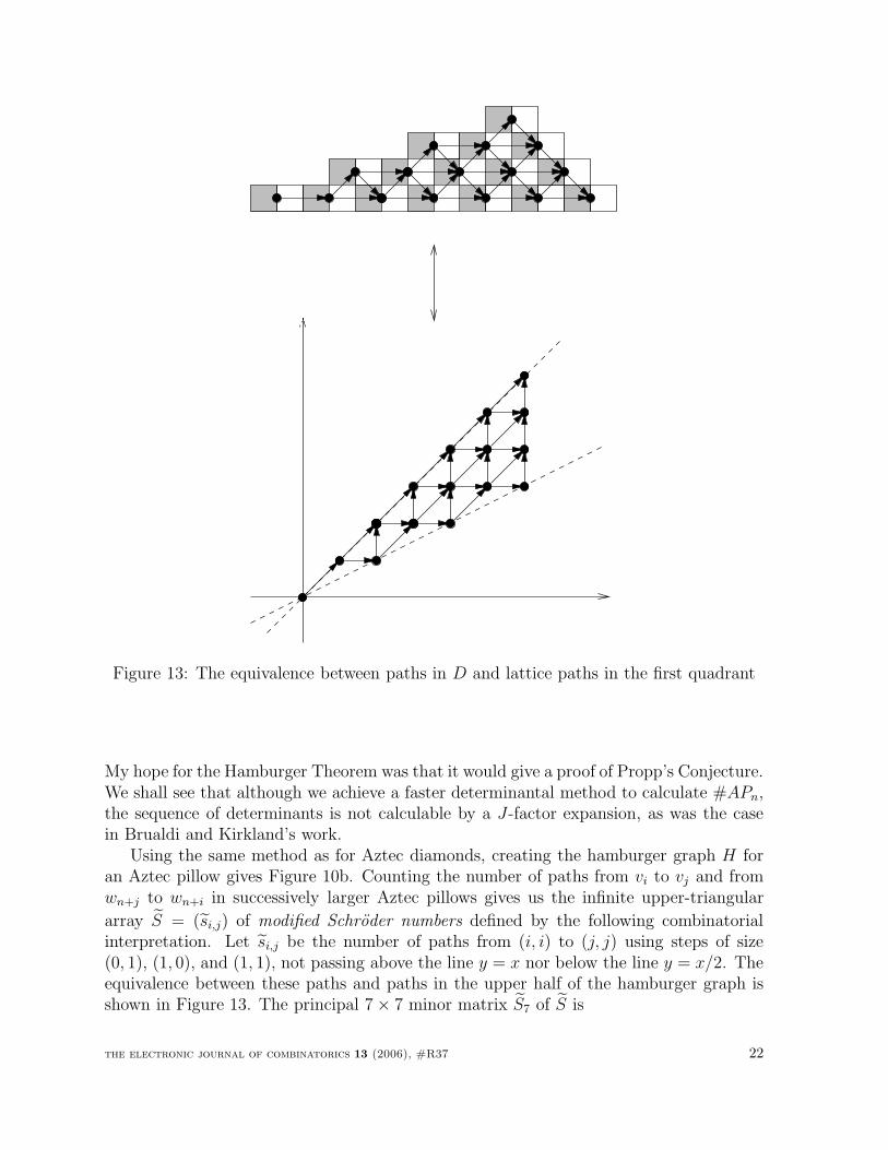
Figure 13: The equivalence between paths in D and lattice paths in the first quadrant

My hope for the Hamburger Theorem was that it would give a proof of Propp’s Conjecture.We shall see that although we achieve a faster determinantal method to calculate #APn,the sequence of determinants is not calculable by a J-factor expansion, as was the casein Brualdi and Kirkland’s work.

Using the same method as for Aztec diamonds, creating the hamburger graph H foran Aztec pillow gives Figure 10b. Counting the number of paths from vi to vj and fromwn+j to wn+i in successively larger Aztec pillows gives us the infinite upper-triangular

array S = (si,j) of modified Schroder numbers defined by the following combinatorialinterpretation. Let si,j be the number of paths from (i, i) to (j, j) using steps of size(0, 1), (1, 0), and (1, 1), not passing above the line y = x nor below the line y = x/2. Theequivalence between these paths and paths in the upper half of the hamburger graph isshown in Figure 13. The principal 7 × 7 minor matrix S7 of S is


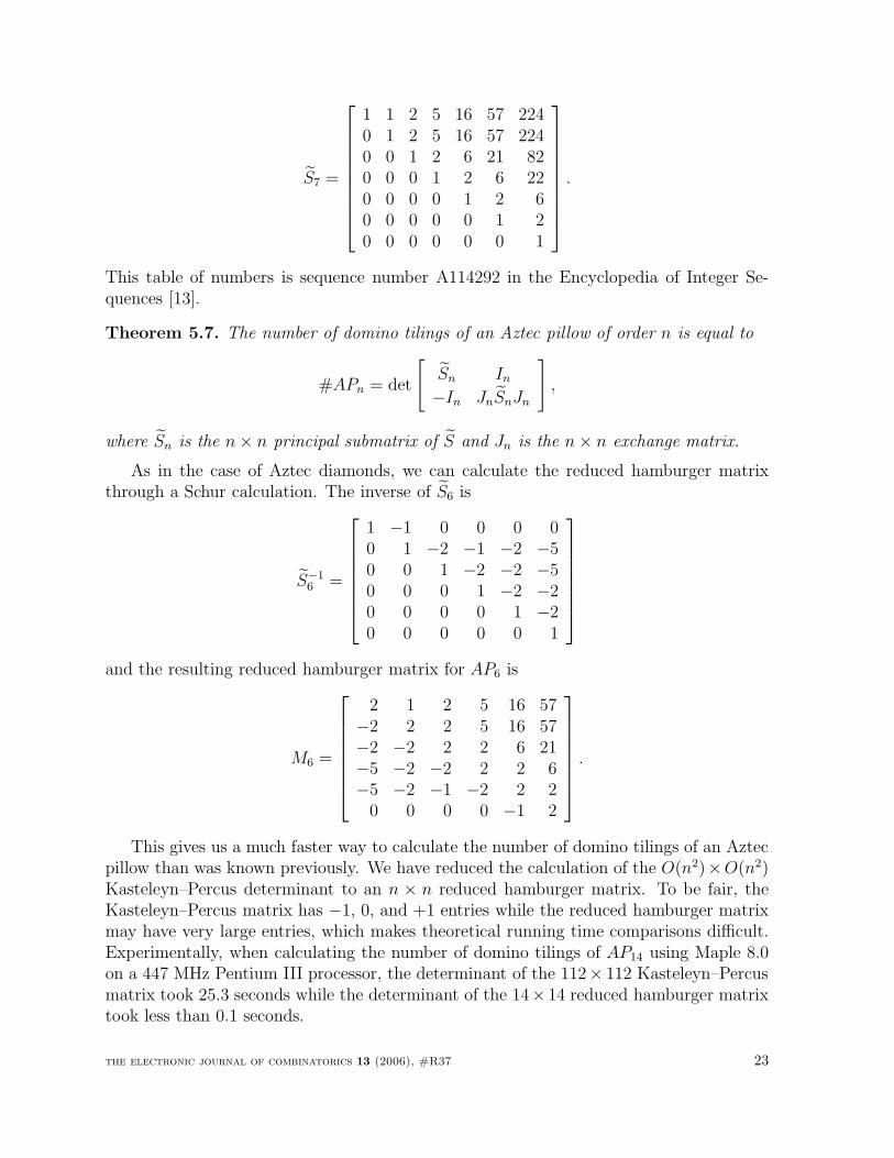
S7 =

1 1 2 5 16 57 2240 1 2 5 16 57 2240 0 1 2 6 21 820 0 0 1 2 6 220 0 0 0 1 2 60 0 0 0 0 1 20 0 0 0 0 0 1

.

This table of numbers is sequence number A114292 in the Encyclopedia of Integer Se-quences [13].

Theorem 5.7. The number of domino tilings of an Aztec pillow of order n is equal to

#APn = det

[Sn In

−In JnSnJn

],

where Sn is the n × n principal submatrix of S and Jn is the n × n exchange matrix.

As in the case of Aztec diamonds, we can calculate the reduced hamburger matrixthrough a Schur calculation. The inverse of S6 is

S−16 =

1 −1 0 0 0 00 1 −2 −1 −2 −50 0 1 −2 −2 −50 0 0 1 −2 −20 0 0 0 1 −20 0 0 0 0 1

and the resulting reduced hamburger matrix for AP6 is

M6 =

2 1 2 5 16 57−2 2 2 5 16 57−2 −2 2 2 6 21−5 −2 −2 2 2 6−5 −2 −1 −2 2 2

0 0 0 0 −1 2

.

This gives us a much faster way to calculate the number of domino tilings of an Aztecpillow than was known previously. We have reduced the calculation of the O(n2)×O(n2)Kasteleyn–Percus determinant to an n × n reduced hamburger matrix. To be fair, theKasteleyn–Percus matrix has −1, 0, and +1 entries while the reduced hamburger matrixmay have very large entries, which makes theoretical running time comparisons difficult.Experimentally, when calculating the number of domino tilings of AP14 using Maple 8.0on a 447 MHz Pentium III processor, the determinant of the 112× 112 Kasteleyn–Percusmatrix took 25.3 seconds while the determinant of the 14×14 reduced hamburger matrixtook less than 0.1 seconds.


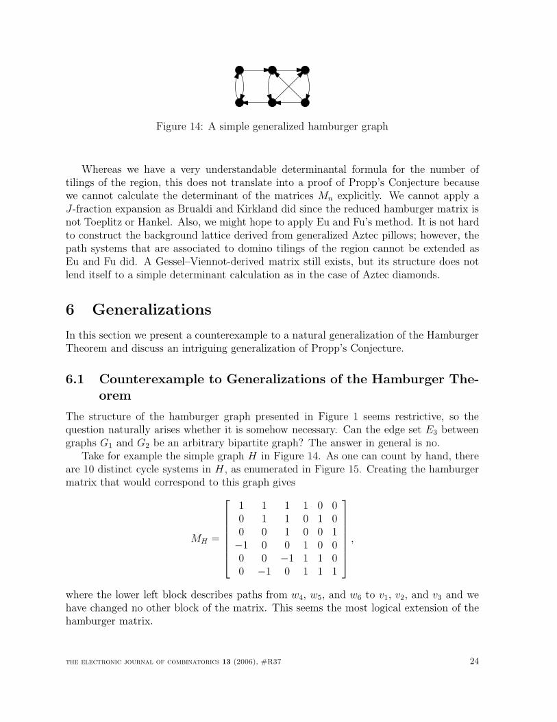
Figure 14: A simple generalized hamburger graph

Whereas we have a very understandable determinantal formula for the number oftilings of the region, this does not translate into a proof of Propp’s Conjecture becausewe cannot calculate the determinant of the matrices Mn explicitly. We cannot apply aJ-fraction expansion as Brualdi and Kirkland did since the reduced hamburger matrix isnot Toeplitz or Hankel. Also, we might hope to apply Eu and Fu’s method. It is not hardto construct the background lattice derived from generalized Aztec pillows; however, thepath systems that are associated to domino tilings of the region cannot be extended asEu and Fu did. A Gessel–Viennot-derived matrix still exists, but its structure does notlend itself to a simple determinant calculation as in the case of Aztec diamonds.

6 Generalizations

In this section we present a counterexample to a natural generalization of the HamburgerTheorem and discuss an intriguing generalization of Propp’s Conjecture.

6.1 Counterexample to Generalizations of the Hamburger The-orem

The structure of the hamburger graph presented in Figure 1 seems restrictive, so thequestion naturally arises whether it is somehow necessary. Can the edge set E3 betweengraphs G1 and G2 be an arbitrary bipartite graph? The answer in general is no.

Take for example the simple graph H in Figure 14. As one can count by hand, thereare 10 distinct cycle systems in H , as enumerated in Figure 15. Creating the hamburgermatrix that would correspond to this graph gives

MH =

1 1 1 1 0 00 1 1 0 1 00 0 1 0 0 1−1 0 0 1 0 00 0 −1 1 1 00 −1 0 1 1 1

,

where the lower left block describes paths from w4, w5, and w6 to v1, v2, and v3 and wehave changed no other block of the matrix. This seems the most logical extension of thehamburger matrix.


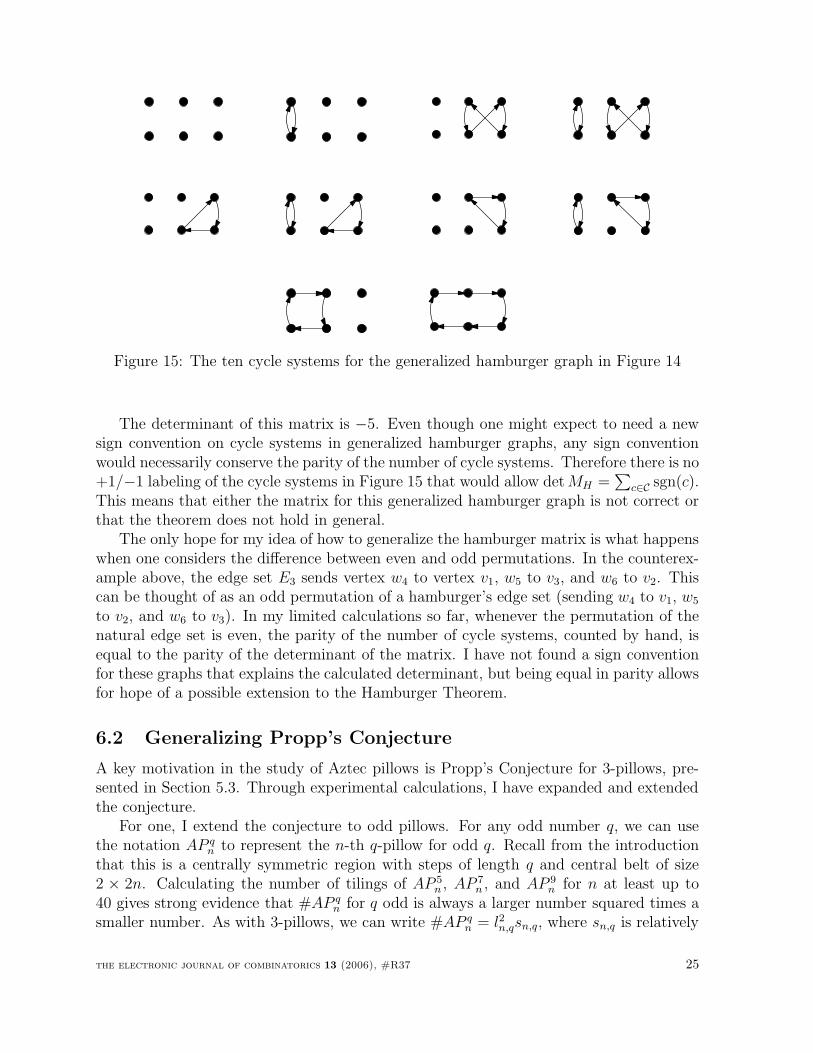
Figure 15: The ten cycle systems for the generalized hamburger graph in Figure 14

The determinant of this matrix is −5. Even though one might expect to need a newsign convention on cycle systems in generalized hamburger graphs, any sign conventionwould necessarily conserve the parity of the number of cycle systems. Therefore there is no+1/−1 labeling of the cycle systems in Figure 15 that would allow det MH =

∑c∈C sgn(c).

This means that either the matrix for this generalized hamburger graph is not correct orthat the theorem does not hold in general.

The only hope for my idea of how to generalize the hamburger matrix is what happenswhen one considers the difference between even and odd permutations. In the counterex-ample above, the edge set E3 sends vertex w4 to vertex v1, w5 to v3, and w6 to v2. Thiscan be thought of as an odd permutation of a hamburger’s edge set (sending w4 to v1, w5

to v2, and w6 to v3). In my limited calculations so far, whenever the permutation of thenatural edge set is even, the parity of the number of cycle systems, counted by hand, isequal to the parity of the determinant of the matrix. I have not found a sign conventionfor these graphs that explains the calculated determinant, but being equal in parity allowsfor hope of a possible extension to the Hamburger Theorem.

6.2 Generalizing Propp’s Conjecture

A key motivation in the study of Aztec pillows is Propp’s Conjecture for 3-pillows, pre-sented in Section 5.3. Through experimental calculations, I have expanded and extendedthe conjecture.

For one, I extend the conjecture to odd pillows. For any odd number q, we can usethe notation AP q

n to represent the n-th q-pillow for odd q. Recall from the introductionthat this is a centrally symmetric region with steps of length q and central belt of size2 × 2n. Calculating the number of tilings of AP 5

n , AP 7n , and AP 9

n for n at least up to40 gives strong evidence that #AP q

n for q odd is always a larger number squared times asmaller number. As with 3-pillows, we can write #AP q

n = l2n,qsn,q, where sn,q is relatively


2.875

2.88

2.885

2.89

2.895

2.9

10 15 20 25 30 35 40

2.8

2.9

3

3.1

3.2

3.3

10 15 20 25 30 35 40

q = 3 q = 5

2.8

3

3.2

3.4

3.6

3.8

4

10 15 20 25 30 35 402.6

2.8

3

3.2

3.4

3.6

3.8

4

4.2

4.4

10 15 20 25 30 35 40

q = 7 q = 9

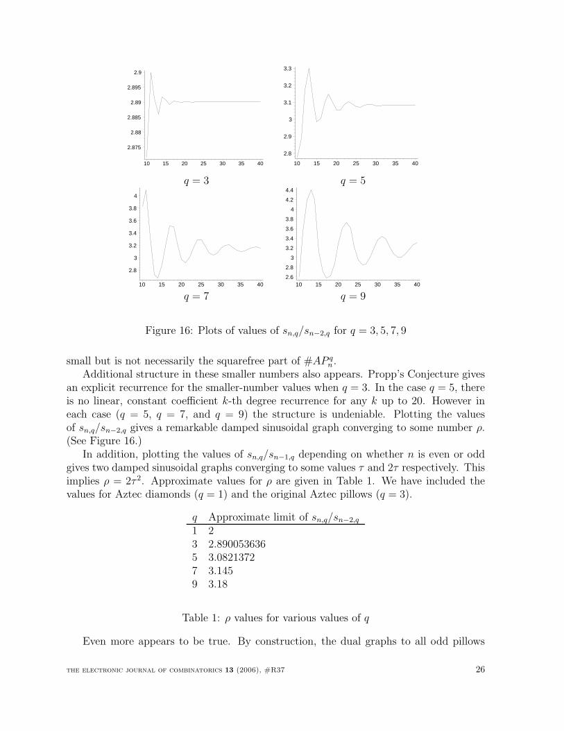
Figure 16: Plots of values of sn,q/sn−2,q for q = 3, 5, 7, 9

small but is not necessarily the squarefree part of #AP qn .

Additional structure in these smaller numbers also appears. Propp’s Conjecture givesan explicit recurrence for the smaller-number values when q = 3. In the case q = 5, thereis no linear, constant coefficient k-th degree recurrence for any k up to 20. However ineach case (q = 5, q = 7, and q = 9) the structure is undeniable. Plotting the valuesof sn,q/sn−2,q gives a remarkable damped sinusoidal graph converging to some number ρ.(See Figure 16.)

In addition, plotting the values of sn,q/sn−1,q depending on whether n is even or oddgives two damped sinusoidal graphs converging to some values τ and 2τ respectively. Thisimplies ρ = 2τ 2. Approximate values for ρ are given in Table 1. We have included thevalues for Aztec diamonds (q = 1) and the original Aztec pillows (q = 3).

q Approximate limit of sn,q/sn−2,q

1 23 2.8900536365 3.08213727 3.1459 3.18

Table 1: ρ values for various values of q

Even more appears to be true. By construction, the dual graphs to all odd pillows


are 2-even-symmetric—that is, centrally symmetric so that antipodes are an even pathlength apart. Jockusch [7] proved that the number of matchings of such a graph G isthe sum of two squares. In terms of the underlying graph, these two squares are thereal and imaginary parts of a weighted matching of the graph G2. If we consider R2 tobe the rotation by 180 degrees, the graph G2 is derived from G by taking a branch cutthrough the graph, removing the vertices on one side of the branch cut, and placing annew edge between any two vertices v and w such that v and R2(w) were connected in G.The weighting gives these new edges the weight i to the power of the net number of timesthe original edge in G crossed the branch cut counterclockwise when traversing from thewhite vertex to the black vertex.

Through a different method in my doctoral dissertation [6], I also showed that thenumber of domino tilings of the region is a sum of two squares. This follows from thestructure of the Kasteleyn–Percus matrix for a rotationally symmetric generalized Aztecpillow. After limited calculation, these two methods appear to give the same sums-of-squares representation. For a q-pillow, we will call these values an,q and bn,q; that is, forany Aztec Pillow, we can write #AP q

n = a2n,q + b2

n,q. Analysis of this set of squares yieldsunexpected information about the larger numbers ln appearing in Propp’s Conjecture,and the larger numbers ln,q in general. For any odd pillow AP q

n , ln,q divides both an,q

and bn,q. This gives us new insight into the structure of the previously ununderstood ln,q,and implies that sn,q is also a sum of squares. Thus, I formulate a new and improvedconjecture about odd pillows.

Conjecture 6.1. The number of tilings of AP qn is a larger number squared times a smaller

number. There exist values ln,q and sn,q such that we can write #AP qn = l2n,qsn,q. The

value sn satisfies the following structure. The ratio of s2n+1,q/s2n,q to s2n+2,q/s2n+1,q isexactly 2 in the limit. In addition, for the values an,q and bn,q in #AP q

n ’s sum-of-squaresrepresentation, ln,q divides both an,q and bn,q.

6.3 Conclusion

The Hamburger Theorem allows us to calculate the number of cycle systems in generalizedAztec Pillow graphs more quickly. It also allows us to count the number of cycle systemsin many previously inaccessible graphs, such as non-planar hamburger graphs. Just asGessel and Viennot’s result has found many applications, I hope the Hamburger Theoremwill be useful as well.

6.4 Remarks

This article is based on work in the author’s doctoral dissertation [6]. A preliminaryversion of this article appeared as a poster at the 2005 International Conference on FormalPower Series and Algebraic Combinatorics in Taormina, Italy. The author would like tothank Henry Cohn and Tom Zaslavsky for numerous intriguing discussions and usefulcorrections. The author would also like to thank an anonymous referee for his or her timeand suggestions for improving this article.


References

[1] Martin Aigner. Lattice paths and determinants. In Computational Discrete Mathe-matics, volume 2122 of Lecture Notes in Comput. Sci., pages 1–12. Springer, Berlin,2001.

[2] Richard Brualdi and Stephen Kirkland. Aztec diamonds and digraphs, andHankel determinants of Schroder numbers. Submitted, 2003. Available athttp://www.math.wisc.edu/∼brualdi/aztec2.pdf.

[3] Sen-Peng Eu and Tung-Shan Fu. A simple proof of the Aztec diamond the-orem. Electron. J. Combin., 12:Research Paper 18, 8 pp. (electronic), 2005.arXiv:math.CO/0412041.

[4] Ira Gessel and Xavier G. Viennot. Binomial determinants, paths, and hook lengthformulae. Adv. in Math., 58:300–321, 1985.

[5] Ira Gessel and Xavier G. Viennot. Determinants, paths, and plane partitions.Manuscript, 1989. Available at http://www.cs.brandeis.edu/∼ira/papers/pp.pdf.

[6] Christopher R. H. Hanusa. A Gessel-Viennot-Type Method for Cycle Systems withApplications to Aztec Pillows, PhD Thesis, University of Washington, June 2005.Available athttp://www.math.binghamton.edu/chanusa/papers/2005/Dissertation.pdf.

[7] W. Jockusch. Perfect matchings and perfect squares. J. Combin. Theory Ser. A,67(1):100–115, 1994.

[8] Samuel Karlin and James McGregor. Coincidence probabilities. Pacific J. Math.,9:1141–1164, 1959.

[9] P. W. Kasteleyn. The statistics of dimers on a lattice I. The number of dimerarrangements on a quadratic lattice. Physica, 27:1209–1225, 1961.

[10] B. Lindstrom. On the vector representations of induced matroids. Bull. LondonMath. Soc., 5:85–90, 1973.

[11] J. Percus. One more technique for the dimer problem. J. Math. Phys., 10:1881–1884,1969.

[12] James Propp. Enumeration of matchings: problems and progress. In New per-spectives in algebraic combinatorics (Berkeley, CA, 1996–97), volume 38 of Math.Sci. Res. Inst. Publ., pages 255–291. Cambridge Univ. Press, Cambridge, 1999.arXiv:math.CO/9904150.

[13] N. J. A. Sloane. The On-Line Encyclopedia of Integer Sequences.http://www.research.att.com/∼njas/sequences/.

[14] Fuzhen Zhang. The Schur Complement and its Applications, volume 4 of NumericalMethods and Algorithms. Springer, New York, 2005.


a gessel{viennot-type method for cycle systems … · a gessel{viennot-type method for cycle...

Documents