Title A GIS-based assessment method for mean radiant temperaturein dense urban areas

Author(s) Huang, J; Cedeño-Laurent, JG; Spengler, J; Reinhart, C

CitationSimbuild 2012 - The 5th National Conference of the InternationalBuilding Performance Simulation Association (IBPSA), Madison,WI., 1-3 August 2012.

Issued Date 2012

URL http://hdl.handle.net/10722/207457

Rights Creative Commons: Attribution 3.0 Hong Kong License

A GIS-BASED ASSESSMENT METHOD FOR MEAN RADIANT TEMPERATURE 1

IN DENSE URBAN AREAS 2

3

Jianxiang Huang, 1

Jose Guillermo Cedeño Laurent, 2

John Spengler, 3

Christoph Reinhart 4

4 1Harvard University Graduate School of Design, Cambridge, MA 5

2Harvard University School of Public Health, Boston, MA 6

3Harvard University School of Public Health, Boston, MA 7

4The Massachusetts Institute of Technology Department of Architecture, Cambridge, MA 8

9

ABSTRACT

The mean radiant temperature (Tmrt) is among

the most important factors affecting thermal

comfort. Its assessment in dense cities has

been complicated due to the presence of

buildings, pavings, and infrastructure. This

paper introduced the RAMUM model, a GIS

based software method developed to simulate

outdoor mean radiant temperature at micro-

scale. The advantages of this method lie in its

efficiency and resolution that supports the

design of buildings, streets, and public open

spaces. The model is evaluated using field

measurements under cold and warm weather

in Boston. This study is sponsored by the

EFRI-1038264 award from the National

Science Foundation (NSF), Division of

Emerging Frontiers in Research and

Innovation (EFRI).

INTRODUCTION

The mean radiant temperature (Tmrt) is among the most

important meteorological factors in relation to human

body energy balance. It is by definition the uniform

temperature of an imaginary enclosure in which radiant

heat transfer from the human body is equal to the

radiant heat transfer in the actual non-uniform

enclosure (ISO, 1998). It is a key variable to thermal

comfort and pedestrian activities (Nikolopoulou and

Lykoudis, 2006), which are essential to the design of

walkable and livable cities that promotes health and

sustainability. There is a practical need for

environmental assessment tools that are both efficient

and supportive of design decisions at micro-scale.

The objective of this paper is to present a software

method to simulate Tmrt in urban environments. The

model is named the Rapid Assessment Method for

Urban Microclimate (RAMUM). It is based on

ArcGIS, the widely used data platform among

researchers and design practitioners. The model

requires minimum input of dry bulb temperature,

relative humidity, 3D buildings and topography

information. It is capable of computing Tmrt for two-

dimensional surfaces at a grid resolution of one meter

by one meter, and the results can be graphically

interpreted on hourly basis. The model is evaluated

using field measurements conducted in Boston,

Massachusetts.

LITERATURE

The assessment of Tmrt has been complex in dense

urban areas, since both shortwave and longwave

radiations are highly varied due to the presence of

buildings, infrastructure, and paving. Several tools

emerged in recent years in an attempt to simulate

radiation influx at the urban scale. Rayman Pro is a

software tool designed for outdoor environmental

analysis. The software is based on a stationery heat

balance model, and it takes into account both short-

wave and long-wave radiation fluxes (Matzarakis,

2007). It requires separate morphological input, and it

can neither process complex building geometries nor

calculate Tmrt on a continuous surface. Similarly,

ENVI-met is a software package capable of simulating

the surface-plant-air interactions in urban

environments. The software applies computational fluid

dynamics (CFD) models and energy balance models

(Bruse, 2006). Like Rayman Pro, ENVI-met is limited

in data input and complex geometries. Others include

the Simulation Platform of Thermal Environment

(SPOTE) (Lin, et al., 2006), the Townscope II (Teller

and Azar, 2001), and the Integrated Environmental

Solutions – Virtue Environment (IES, 2012).

Despite the rising importance in sustainable design and

occupant comfort, environmental assessment tools are

rarely used in planning and urban design practices.

Barriers persist between researcher and practitioners,

and existing tools are often limited in model input, data

exchange, and visualization capacities. To better serve

the needs of urban designers and planners, the

simulation model should be computationally efficient,

transparent, and graphically intuitive. It should support

information exchange with other simulation packages

as well as database platform such as the Geographic

Information System (ESRI, 2012), a widely used

software among design practitioners.

Figure 1. The mean radiant temperature at 1.5 meters

height above ground

METHOD

By definition, the calculation of Tmrt can be expressed

with the following formula (Fanger, 1970)

4n-p

4

nn2-p

4

221-p

4

11mrt )·F·T + … + ·F·T + ·F·T( = T εεε

(1)

εn = Emittance for surface materials (ratio)

Tn = Temperature of isothermal surfaces

Tn = View factor of isothermal surfaces

In real urban context, it is impractical to estimate

temperature for every isothermal surface. A simplified

approach separates radiation into three components:

shortwave radiation; longwave radiation from the sky;

and longwave radiation from solid surfaces, in this case

the ground and the buildings. The alternative formula is presented below and the calculation for each of the

three components will be explained in detail.

4ggpaapsmrt )·FE + ·FE + ·FE(

1 = T ⋅⋅⋅ εε

σska

(2)

σ = Stephan-Bolzmann Constant

(5.67·10−8

W/m2K

4)

ak = Absorption coefficient of shortwave radiation

for the target object (standard value 0.7)

εp = Emission coefficient for the target object

(standard value 0.97)

Ea = Longwave radiation intensity of the open sky

(W/m2)

En = longwave radiation intensity of solid surfaces

(W/m2)

Fs,a,g = angle factors of the sky, solar radiation, and

solid surfaces (ratio)

The target object for this study is a 40mm grey ball

thermometer placed at 1.5 meter above the ground, an

approximate of human body. The model also uses

weather data from the nearest station, in this case the

portable weather station present on site is brought into

use. The workflow is automated using the programming

language of Python. The results are presented in

ArcScene at a grid resolution of one meter by one

meter. (Figure 1)

Shortwave Radiation

Shortwave radiation can be simulated using DIVA-for-

Rhino 2.0 (Jakubiec and Reinhart, 2011), an advanced

daylight simulation tool based on Radiance, Daysim

(Reinhart and Walkenhorst, 2001) and Rhinoceros 10

interface (McNeel, 2012). The hourly radiation data is

downloaded from the Central Square weather station

located in Cambridge, MA (Wview, 2012) Three-

dimensional urban models of the study area are

acquired from Boston Redevelopment Authority (BRA,

2011).

DIVA-for-Rhino calculates hourly the global horizontal

irradiance for sensor grids of one meter by one meter.

The results are imported to raster layers in ArcGIS.

The base map information, including building

footprint, road, are acquired from the Office of

Geographic Information (MassGIS, 2011).

Figure 2, Shortwave radiance Es of 1m grid resolution,

reflectance = 0.35. Hourly calculation conducted

using DIVA-for-Rhino Plug-in, based on 3D urban

model acquired from the Boston Redevelopment

Authority and Massachusetts Office of Geographic

Information.

Notice that DIVA-for-Rhino calculates global

horizontal radiance received from a planar surface

facing upwards. For a spherical surface, the results can

be approximated with homogeneous radiation with the

angle factor Fs= 0.5. The percentage of error is

expected to increase when the solar angle is low. Yet

the absolute error will become negligible compared

with intrinsic errors imbedded in solar radiation

simulation models at low-solar angles (Ibarra and

Reinhart, 2011)

Longwave Radiation from the Sky

The radiation from the sky can by estimated using the

Angstrom formula: (Falkenberg and Bolz

1949;Monteith 1990; Oke 1987; VDI 1994):

))8

(21.01()1025.082.0()15.273( 5.20945.04 NTE pV

aa ⋅+⋅⋅−⋅+⋅=⋅−

σ

(3)

Ea = Longwave radiation from the sky (W/m2)

Ta = Dry bulb temperature (°C)

N = Degree of cloudiness (octas)

Vp = Vapor pressure (hPa)

The vapor pressure Vp is computed using Arden Buck

equation (Buck,1981)

))14.257

()4.234

678.18exp((1121.6a

aa

humpT

TTRV

+

⋅−⋅=

(4)

Vp = The saturation vapor pressure in hPa

Rhum = Relative humidity (%)

Ta = Dry bulb temperature (°C)

For spherical surface, the angle factor of longwave

radiation from sky can be conveniently determined

from sky view factor

Fa = SVF / 2

SVF = Sky view factor from the center of the grid cell

The sky view factor can be calculated from DIVA-for-

Rhino plug-in based on Radiance. Ambient bounces

were set equal to one (ab = 1) and run a daylight factor

simulation for grid sensors under the uniform sky. The

result is imported to ArcGIS using Python

programming language. (Figure 3)

Figure 3. Sky View Factor, calculated using DIVA-for-

Rhino Plug-in, plotted from ArcGIS

Longwave Radiation from Solid Surfaces

The longwave radiation from the ground and buildings

is determined by aggregate longwave radiation from

each isothermal surface as well as those reflected from

the sky:

⋅⋅−+

=

∑

∑

=

=

n

i

i

n

i

iaii

g

F

FEE

E

1

1

))1(( ε

(5)

Ei = longwave radiation from surface (W/m2)

εi = Emittance of surface material

Ea = Longwave radiation from the sky (W/m2)

Fi = Angle factor of solid surface (ratio)

The longwave radiation emitted by individual surfaces

can be expressed by Stephan-Bolztmann’s law: 4

sii TE ⋅⋅= σε

σ = Stephan-Bolzmann Constant (5.67·10−8

W/m2K

4)

εi = Emittance of surface material,

Ts = Temperature of solid surface

The temperature of solid surfaces, in this case building

facades and ground paving, is jointly determined by air

temperature, ambient radiation, indoor temperature,

and the insulation value of surface materials. The

building façades on site consist mostly of stone and

concrete surfaces, which reduces uncertainties

associated with longwave radiation through glazing.

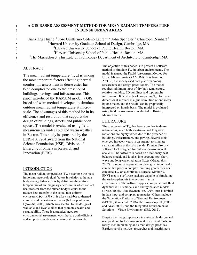
Infrared photographs were taken at each hour to record

solid surface temperatures of the ground and building

façade. data suggests that the temperature of individual

surfaces could vary up to 20 degrees from the air

temperature. However, the mean temperature of all

solid surfaces matches closely with the air temperature

with small margins of error (Figure 4). For

simplification purposes, it is therefore reasonable to

assume isothermal conditions for all solid surfaces in

the model with temperature equal to those of the

ambient air. Given Ts = Ta, and for most building

materials ε ≈ 1, a simplified formula can be expressed

below

4

ag TE ⋅= σ (6)

σ = Stephan-Bolzmann Constant

(5.67·10−8

W/m2K

4)

Ta = Dry bulb temperature (°C)

Mean Temperature of the Air and Solid Surfaces

-25

-20

-15

-10

-5

0

7:15

7:40

8:05

8:30

8:55

9:20

9:45

10:1

0

10:3

5

11:0

0

11:2

5

11:5

0

12:1

5

12:4

0

13:0

5

13:3

0

13:5

5

14:2

0

14:4

5

15:1

0

15:3

5

16:0

0

16:2

5

Hour

Te

mp

era

ture

C

Air Surface (mean) Ground East Façade

North Façade South Façade West Façade

Figure 4, the air temperature of the dry bulb matches

closely with the average temperature of solid surfaces.

Façade/ground temperature estimated using hourly

infrared photography (Figure 10).

MEASUREMENT

The above simulation results are evaluated using field

measurement conducted on January 15 and March 21,

2012 respectively. These experiment dates are chosen

to maximize temperature range. The former, Jan.15 is a

cold day with low air temperature recorded from -18 to

-8 degrees centigrade. In contrast, March 21 is an

exceptionally warm day with recorded air temperature

betwen 15 and 25 degrees centigrade during the day.

Both days are mostly clear except for a few hours of

cloudiness in the afternoon of Jan.15.

Figure 5. Measurement Site, Countway Library

Courtyard, Harvard University, Boston, MA

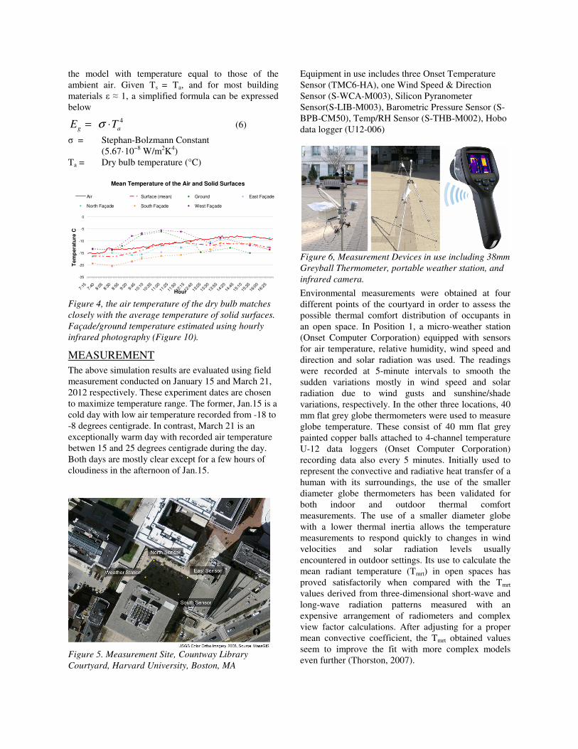
Equipment in use includes three Onset Temperature

Sensor (TMC6-HA), one Wind Speed & Direction

Sensor (S-WCA-M003), Silicon Pyranometer

Sensor(S-LIB-M003), Barometric Pressure Sensor (S-

BPB-CM50), Temp/RH Sensor (S-THB-M002), Hobo

data logger (U12-006)

Figure 6, Measurement Devices in use including 38mm

Greyball Thermometer, portable weather station, and

infrared camera.

Environmental measurements were obtained at four

different points of the courtyard in order to assess the

possible thermal comfort distribution of occupants in

an open space. In Position 1, a micro-weather station

(Onset Computer Corporation) equipped with sensors

for air temperature, relative humidity, wind speed and

direction and solar radiation was used. The readings

were recorded at 5-minute intervals to smooth the

sudden variations mostly in wind speed and solar

radiation due to wind gusts and sunshine/shade

variations, respectively. In the other three locations, 40

mm flat grey globe thermometers were used to measure

globe temperature. These consist of 40 mm flat grey

painted copper balls attached to 4-channel temperature

U-12 data loggers (Onset Computer Corporation)

recording data also every 5 minutes. Initially used to

represent the convective and radiative heat transfer of a

human with its surroundings, the use of the smaller

diameter globe thermometers has been validated for

both indoor and outdoor thermal comfort

measurements. The use of a smaller diameter globe

with a lower thermal inertia allows the temperature

measurements to respond quickly to changes in wind

velocities and solar radiation levels usually

encountered in outdoor settings. Its use to calculate the

mean radiant temperature (Tmrt) in open spaces has

proved satisfactorily when compared with the Tmrt

values derived from three-dimensional short-wave and

long-wave radiation patterns measured with an

expensive arrangement of radiometers and complex

view factor calculations. After adjusting for a proper

mean convective coefficient, the Tmrt obtained values

seem to improve the fit with more complex models

even further (Thorston, 2007).

To compensate for the convective and conductive heat

losses from 40 mm grey ball thermalmeter to the air,

the following formula is used to adjust for globe

thermometer reading. (Kuehn, 1970)

15.273)(101.1

)15.273(44.0

6.084

−−⋅

⋅

⋅⋅++= ag

agmrt TT

D

VTT

ε

(7)

Tg= Globe Temperature (°C)

Va= Wind speed (m/s)

Ta= Air Temperature

D = Globe diameter (40mm)

ε = Globe Emittance, 0.97

This inexpensive solution of using globe temperature

measurements has also proven to be a good predictor of

outdoor thermal comfort. A multinational study

performed in several European cities (Nikolopoulou

and Lykoudis, 2006) found the correlation between the

globe temperature and the Actual Sensation Vote

(ASV) responses of study participants to be the highest

among all environmental measurements recorded

(R=0.53), when compared to air temperature (R=0.43),

solar radiation (R=0.23) and wind speed (R=0.26).

These studies confirm the usefulness of the globe

thermometers to approximate the heat transfer of

individuals with the built environment in open spaces.

UNCERTAINTIES

The simulated and measured Tmrt during the experiment

are plotted in figure 7. The 157 pairs of data entries

feature a correlation coefficient of 0.964, while the

differences are normally distributed (Figure 8). A

further breakdown shows the simulation tends to

overestimate the Tmrt by 1~2°C during warm weather

and underestimate the Tmrt by 1~2°C during cold

weather. The sources of uncertainties stem from

building geometries, surface temperature variations,

and measurement errors.

A major source of uncertainties is from the 3D building

database. Different from the simplifed building

geometries in the GIS database, architectural details

such as exterior wall profile, windows extrution,

androof top structures can change the shape of

shadows, resulting in a shift of peak value as it is

observed in figure 12 and 13. Many of the outlyers in

figure 7 with up to 20°C differences between

measurement and prediction can be explained by this

cause.

-40

-20

0

20

40

60

80

100

-40 -20 0 20 40 60 80 100

Simulation MRT C

Me

as

ure

d M

RT

C

East_Jan East_Mar South_Jan South_Mar West_Mar North_Jan North_Mar

Figure 7. Scatter Plot of Measured Tmrt against

Predicated Tmrt. on both Jan. 15 and Mar.21, 2012.

Measurement interval = half hour. Observations n =

157; Correlation coefficient r = 0.964

0

5

10

15

20

25

30

-24 -22 -20 -18 -16 -14 -12 -10 -8 -6 -4 -2 0 2 4 6 8 10 12 14 16 18 20 22 24 More

Tmrt Measurement - Simulation

Ob

serv

ati

on

Co

un

ts

Jan Mar

Figure 8, the distribution of differences between

measured and predicted Tmrt on Jan.15 and Mar.21

A second source of uncertainties comes from

temperature variation of solid surfaces, mostly due to

solar exposure, thermal bridges, or glazing. Figure 9

presented an estimation of the Tmrt in square-shaped

courtyard resembling the countway library site.

Calculation using Fanger’s formula above yeilded a

Tmrt difference of 1.2°C, a noticable but minor error

compared with other sources of uncertainties. Assume

global horizontal shortwave radiation to be 600 W/m2

and the longwave radiation from the sky to be 200

W/m2. The surface temperature of the two solid wall

(highlighted in red) are allowed to vary by 10°C higher

than those of the others.

Figure 9, the heated wall surfaces can raise the Tmrt by

1.2 °C. The calculation is based on a courtyard space

enclosed by walls and floor with a sky view factor of

0.33 from the center. The left scenario assume an

equal temperature to all solid surfaces, while the right

scenario allows the surface temperature of two solid

wall surfaces to rise by 10 °C, the typical differences

observed during the experiment.

Aside from simulation uncertaities, measurement are

also vulnerable to errors from equipment such as the

greyball thermometers. These errors may be further

amplified by Kuehn’s formula when adjusting for

convective heat losses. Further field measurement work

are scheduled in order to test the model’s applicability

in hot climate and under complex weather conditions.

CONCLUSION

The simulation-based method is a useful tool for

estimate radiation fluxes at a spatial resolution that

informs design deicisions. It is capable of performing

rapid analysis in two dimensional. The method requires

minimum input of GIS geospatial information as well

as meteological data. Since the Tmrt is a key estimator

of thermal comfort in outdoor space, this simulation

method will become a useful tool for design and

planning practices. It allows early-phase diagnosis of

undesirable radiant fluxes, which will later inform

choices on building envelope, shading devices, and

vegetation. It can also inform the seleciton of building

and paving materials based on thermal properties, the

reflectance, emittance, and heat capacity. The model

will also support decisions on whether radiant heating

or cooling are needed during extreme weather events.

A following application of the model is to calculate

outdoor thermal comfort in dense urban spaces. The

Tmrt, along with wind speed, air temperature, and

humidity, constitutes the key meteological inputs for

thermal comfort metrics.

REFERENCES

McNeel, R. 2010. Rhinoceros - NURBS Modeling for

Windows (version 4.0), McNeel North America,

Seattle, WA, USA. (www.rhino3d.com/)

ASHRAE. 2001. ASHRAE Fundamentals Handbook

2001 (SI Edition) American Society of Heating,

Refrigerating, and Air-Conditioning Engineers,

ISBN: 1883413885.

Azar S. 2006. TownScope III, University of Liege,

Belgium. http://www.townscope.com.

Buck, A. L. 1981, "New equations for computing vapor

pressure and enhancement factor", J. Appl.

Meteorol. 20: 1527–1532

Bruse M. 2006. ENVI-met 3 – a three dimensional

microclimate model. Ruhr Universit¨at Bochum,

Geographischer Institut, Geomatik.

http://www.envi-met.com

ESRI, The GIS software. http://www.esri.com/

Fanger, P.O. 1970, Thermal Comfort: Analysis and

Applications in Environmental Engineering,

McGraw-Hill Book Company, New York.

Ibarra, Diego; Reinhart, Christoph, 2011, Solar

availability: A comparison study of irradiation

distribution methods, Building Simulation 2011,

Sydney, Australia.

Integrated Environment Solutions:

http://www.iesve.com/

International Organization for Standardization, 1998.

Ergonomics of the thermal environment -

Instrument for measuring physical quantities.

Geneva, Switzerland. ISO 7726.

Jakubiec, J A; Reinhart, C F "DIVA-FOR-RHINO 2.0:

Environmental parametric modeling in

Rhinoceros/Grasshopper using Radiance, Daysim

and EnergyPlus", Conference Proceedings of

Building Simulation 2011, Sydney, Australia.

Kuehn LA, Stubbs RA, Weaver RS. 1970. Theory of

the globe thermometer. Journal of Applied

Physiology 29: 750–757.

Lagios, K; Niemasz, J and C F Reinhart, 2010,

Animated Building Performance Simulation

(ABPS) - Linking Rhinoceros/Grasshopper with

Radiance/Daysim, the Proceedings of SimBuild

2010, New York

Lin, Borong; Zhu, Yingxin; Li, Xiaofeng; Qin,

Youguo; 2006, Numerical simulation studies of the

different vegetation patterns’ effects on outdoor

pedestrian thermal comfort. The Forth

International Symposium on Computational Wind

Engineering, Yokohama, Japan

Nikolopoulou, M. and Lykoudis, S., 2006. Thermal

comfort in outdoor urban spaces: Analysis across

different European countries. Building and

Environment, 41 (11), pp. 1455-1470.

Reinhart C. F. and Walkenhorst O. (2001) Validation

of dynamic RADIANCE-based daylight

simulations for a test office with external blinds.

Energy and Buildings 33, 683-697.

Steel,Mark,2011,wview:http://www.wviewweather.com

The Boston Redevelopment Authority,

http://www.bostonredevelopmentauthority.org/Ho

me.aspx

The Common Wealth of Massachussetts, Office of

Geographic Information (MassGIS)

http://www.mass.gov/mgis/massgis.htm

Thorsson,S., Lindberg, F., Eliasson, I., and Holmer, B.,

2007. Different methods for estimating the mean

radiant temperature in an outdoor urban setting.

International Journal of Climatology, 27, pp.1983–

1993

APPENDIX A

Figure 10, Hourly temperature of solid surfaces based

on infrared photograph, January 15, 2012

APPENDIX B

Figure 11. Simulation of Mean Radiant Temperature on Countway Library Courtyard, January 15, 2012. Grid

dimension, 1m by 1m. For concrete façade and pavings materials, albedo = 0.35, emissivity = 1

-20

-15

-10

-5

0

5

10

15

20

25

30

7:15 7:40 8:05 8:30 8:55 9:20 9:45 10:10 10:35 11:00 11:25 11:50 12:15 12:40 13:05 13:30 13:55 14:20 14:45 15:10 15:35 16:00

Time

Tem

pera

ture

C

South Measur. North Measur. East Measur. Air Temp. East Sim North Sim South Sim

Figure 12. Predicted and Measured Tmrt on Jan.15. Isolated points are extracted from simulation results, while

continuous curves are from measurement data using a 40 mm grey globe thermometer.

0

10

20

30

40

50

60

70

80

7:30 8:00 8:30 9:00 9:30 10:00 10:30 11:00 11:30 12:00 12:30 13:00 13:30 14:00 14:30 15:00 15:30 16:00 16:30 17:00 17:30 18:00 18:30 19:00

Time

Te

mp

era

ture

CEast Measur. South Measur. West Measur. North Measur. Air Temp. East Sim South Sim West Sim

Figure 13. Predicted and Measured Tmrt on Mar.21. Isolated points are extracted from simulation results, while

continuous curves are from measurement data using a 40 mm grey globe thermometer.