a gps-reﬂections receiver that computes doppler/delay …

156 IEEE TRANSACTIONS ON GEOSCIENCE AND REMOTE SENSING, VOL. 45, NO. 1, JANUARY 2007

A GPS-Reflections Receiver That ComputesDoppler/Delay Maps in Real Time

Oleguer Nogués-Correig, Estel Cardellach Galí, Josep Sanz Campderrós, and Antonio Rius

Abstract—This paper describes a new instrument that was spe-cially designed and developed to gather global positioning system(GPS) signals after they have been reflected from suitable sur-faces (sea, ice, and ground), for Earth remote sensing. The devicehas been called the GPS open-loop differential real-time receiver(GOLD-RTR). Its main and most innovative feature is its compu-tation and storage, in real time, of complex-valued (I and Q) crosscorrelations (waveforms) between GPS L1-C/A signals—receiveddirectly and after reflection—and the corresponding models ofthese signals. Particularly, the GOLD-RTR schedules consecutivecoherent integration time slots of 1 ms over which ten parallel cor-relation channels, with 64 lags each, work simultaneously and con-tinuously with the input raw data sampled at 40 MHz. The totalthroughput is 10 000 waveforms per second, each waveform being64 lags long. These real-time correlation resources can be flexiblydistributed in several configurations according to the observa-tional requirements, for instance: Doppler/delay maps or up to tensimultaneous reflected waveforms for ten different GPS satellitesare examples of what can be done. The further processing of thereal-time computed 1-ms waveforms in a flight campaign over theocean, ice, or ground can be used to obtain geophysical parameterssuch as sea level and tides, sea surface mean-square slopes, iceroughness and thickness, soil moisture and biomass, or futureapplications. This paper covers the GOLD-RTR architecture andhardware, signal processing and data storage issues, machine–userinterface, laboratory readiness tests, and waveform data samplesfrom the first two jet aircraft campaigns at 9300 m over the sea.

Index Terms—Altimeter, bistatic radar, global positioningsystem reflections (GPS-R), GPS open-loop differential real-timereceiver (GOLD-RTR), passive reflectometry and interferometrysystem (PARIS) concept, radar systems, real-time correlation,scatterometer, waveforms.

I. INTRODUCTION

THE WORKING principle of radar systems is the obser-vation of electromagnetic radiation, scattered from dis-

tant objects that have been illuminated by a radiating sourcein order to remotely study certain physical properties of theobject. Ever since the first monostatic radars appeared, thescattering process of electromagnetic energy from objects hasbeen extensively studied, with applications in the field of Earthremote sensing and in the exploration of other planets andmoons of the solar system [1]. The global positioning system

Manuscript received March 2, 2006; revised July 14, 2006. The campaignswere funded in part by the Spanish National Space Plan (ESP2004-00671,ESP2005-03310).

O. Nogués-Correig, E. Cardellach Galí, and A. Rius are with the Institut deCiencies de l’Espai, Institut d’Estudis Espacials de Catalunya (CSIC-IEEC),08193 Barcelona, Spain (e-mail: [email protected]).

J. Sanz Campderrós was with the Institut de Ciencies de l’Espai, Institutd’Estudis Espacials de Catalunya (CSIC-IEEC), 08193 Barcelona, Spain. He isnow with ENFASYSTEM S.L., 08030 Barcelona, Spain.

Digital Object Identifier 10.1109/TGRS.2006.882257

Fig. 1. Passive reflectometry and interferometry system (PARIS) scenariosketch [2]. A vehicle flying at a certain speed over the ocean observes thenavigation signals emitted by GPS satellites, both direct rays and forward-scattered rays after they are reflected on the sea surface. The difference intime of arrival (TOA) between direct and reflected signals provides informationabout altimetry, whereas the shape of the reflected signal provides informationabout sea surface characteristics.

(GPS) open-loop differential real-time receiver (GOLD-RTR)instrument described in this paper has been developed to ob-serve the navigation signals emitted by GPS satellites, bothdirect rays propagated through the line of sight (LOS) and re-flected forward-scattered rays from the Earth’s surface (bistaticgeometry). This configuration was first proposed in 1993 by theEuropean Space Agency (ESA) as a passive multistatic radarto monitor mesoscale ocean altimetry [2]. Such a scenario isdepicted in Fig. 1. From then on, in-depth work has beenperformed to study the strong points and applications of GPS-reflections (GPS-R). The focus of this work has been in:1) altimetry experiments using models of the envelope of thereflected signals, either from a static position [3] or fromaircraft altitudes [4]–[7]; 2) altimetry experiments that mainlyuse information from the less noisy phase of the reflected signalinstead of the envelope, both from static positions near thereflective surface [8]–[13] or from a Low Earth Orbiter (LEO)altitude using data from the Challenging Minisatellite Payloadfor Geophysical Research and Application (CHAMP) GPSradio occultations satellite [14]; 3) scatterometry experiments toretrieve ocean surface states [15] such as wind [16]–[18] or searoughness [19]; 4) basic theoretical models that describe the de-pendence of sea roughness on wind [20], scatterometric modelsthat describe the dependence of the GPS-reflected signal shapeon wind [21]–[24], and theoretical studies of the polarizationproperties of the GPS-reflected signals [25]; 5) applications forthe characterization of soil moisture [26] and sea ice [27]; andfinally, 6) space observations of GPS-R, first analyzing a fewseconds of the Spaceborn Imaging Radar version C (SIR-C)

0196-2892/$25.00 © 2007 IEEE

NOGUÉS-CORREIG et al.: GPS-REFLECTIONS RECEIVER THAT COMPUTES DOPPLER/DELAY MAPS IN REAL TIME 157

calibration data [28], later using GPS radio occulation datafrom the CHAMP mission [14], [29] and even a dedicatedGPS-R instrument aboard the U.K. Disaster Monitoring Con-stellation (UKDMC) satellite [30], providing the best opportu-nity thus far to observe GPS-R from space. This brief summaryclearly shows that the emphasis has been put on the basicscientific demonstration of the possibilities of GPS-R. Specificinstrumental developments, necessary to obtain more and betterquality data, have received less attention. The GOLD-RTR aimsto fill this gap and substantially improve GPS-R instrumenta-tion. In order to highlight the differences and improvementsbetween GOLD-RTR and previous instrumentation, a reviewof the latter is provided. From now on, it will be assumed thatthe reader is familiar with the GPS system and the structureof its navigation signals. A good summarized review of GPSreceivers and signal structure can be found in [31], or [32],which is more extensive. For a precise official information onGPS user interface specification, refer to [33] and [34].

II. PREVIOUS INSTRUMENTATION

Previous GPS-R instrumentation can be divided into twogroups: software receivers and hardware receivers. The archi-tecture of software receivers is built around a set of multipleradio-frequency (RF) front-ends, which are all supplied by thesame local oscillator (LO) for coherent conversion to base-band (BB). After the analog-to-digital (A/D) conversion andsampling, all the raw signal samples are directly dumped ina mass-storage medium without any kind of cross-correlationprocessing. This processing takes place offline in the laboratory,after the experiment, using dedicated software routines. Theprocessing consists of cross-correlating the raw signals withlocal GPS ranging-signal replicas of the pseudorandom noise(PRN) codes, appropriately frequency shifted to account for theDoppler shift and LO residuals of the received signal. This iscalled the preprocess or correlation process and is performedusing software on a standard computer with the experimentalraw data retrieved from the files. The resulting products ofthis process are closely spaced samples of the cross-correlationfunction, evaluated over a few chips of PRN code aroundthe correlation power peak, forming the so-called waveforms,which are actually the signals used for geophysical exploitation.The following are examples of software receivers:

1) ESA instrumentation-A, based on the GEC-Plessey GPSdevelopment kit [35] for conversion to BB and sam-pling (the same downconversion approach as in Na-tional Aeronautics and Space Administration (NASA)Langley Research Center instrumentation, see below) anda Signatec data acquisition (DAQ) card with 32 MB of runrecording capacity. With this amount of memory, it wasonly possible to acquire continuous raw data in blocks of2.56 s. After each acquisition, data were dumped from theDAQ to a digital tape. Each dump operation took about10 min, thus enabling to record about 80 s of cumulativedata after 4–5 h of continuous operation. An experimentusing this setup is reported in [3].

2) Jet Propulsion Laboratory (JPL) NASA instrumentation,based on modified TurboRogue GPS receivers [36], [37]

that provided the I and Q components of both the L1and L2 GPS signals. The raw sampled data for boththe direct and reflected signals was first synchronouslyand continuously recorded to a SONY SIR-1000 recorder[38], and later onto the hard disk, with virtually no limita-tion on data recording lengths. Specific software routinesimplementing a full GPS software receiver were alsoavailable during the postprocessing stage. A completedescription of this instrument is found in [39], while[5] describes the experiments and results achieved inimplementation.

3) ESA instrumentation-B was used on several experimentsin [6], [7], and [10], based on modified TurboRogue GPSreceivers and two SONY SIR-1000 recorders (similar toJPL’s). This setup recorded only the I component of theBB signal. Moreover, certain sophisticated procedureswere necessary in order to time-align the direct andreflected raw signals, which were dumped to two separatemanually operated recorders.

4) Versatile GPS receiver developed by the Johns HopkinsUniversity Applied Physics Laboratory. The systemfront-end is a GEC-Plessey chip [35], and direct andreflected data were synchronously sampled at 5.714 MHzby a high-speed recording system. Upon postprocessing,a software-based GPS receiver (with delay and Dopplertracking capabilities) was applied to both direct and re-flected signals to obtain the waveforms. A description ofthis software receiver can be found in [40], while [24] and[41] describe an analysis of experimental data collectedby this system.

5) Catalan Institute for Space Studies (IEEC) instrumenta-tion, which was designed and built from scratch by thePolytechnic University of Catalunya (UPC, Barcelona,Spain). Its features are similar to JPL NASA Instrumen-tation, only differing in that it is integrated and assembledin a small and portable 12-kg rack and that it doesnot have L2 frequency signals. Specific software GPSreceiver routines were written for processing the L1, C/Acodes. A description of the system’s hardware is found in[42], while [12] reports on experimental data and resultsachieved with it. The instrument data recording hardwareis covered by a Spanish patent [43].

6) University of Colorado (at Boulder) instrumentation,based on two small GPS antennas mounted at the top andbottom of an aircraft to gather direct and reflected signals.Signals are down-converted to BB, raw sampled, andstored to hard disk drives for postprocessing. A referenceto this system can be found in [44].

7) Starlab Oceanpal instrumentation based on two antennasmounted above and below a circular metallic groundplane, which is sustained near the coast, in order toseparately pick up the direct and reflected signals overthe ocean. The system has two analog downconversionchains and a raw data sampler system at 16 MHz. Recordlengths of raw data are performed and stored on a datamanagement unit. On completing a record, this unit auto-matically computes the complex waveforms and analyzesit further to derive geophysical products. The system is


connected to the web, so the results are available online.A description of this system can be found in [45].

8) Surrey Satellite Space Center (SSTL) instrumentation,which was flown in the UKDMC LEO satellite as anopportunity instrument for gathering GPS-R from space.The instrument is based on a GEC Plessey GPS chipset [35], and the raw sampled data are stored in a massmemory to later be downloaded to Earth for postprocess-ing. A description of this instrument, as well as somepreliminary results, can be found in [30].

9) NAVSYS Corporation has developed several instrumentsbased on one or more digital front-ends (DFEs) and ahigh-speed recording system. One of the latest develop-ments consists of an antenna array of 109 elements [46].The RF output of each antenna array is digitized byDFE and stored to a high-speed recording system. Uponpostprocessing, a digital antenna beam steering and cor-relation process is performed using software. This systemis capable of simultaneous multibeam steering, with theadvantage of having a greater antenna gain.

There are clearly major differences in performance, capacity,and scope between the reviewed software receivers. However,the main limitation is still the fact that: they all require anintensive cross-correlation postprocess which involves the useof software routines, a good knowledge of how to operate themproperly with the raw recorded data, and a considerable amountof time to run these routines and obtain results (at least whenrunning on a standard computer). This is not a comfortableframework for the scientific end user, whose main interest isthe analysis of the observable data: the waveforms obtainedafter postprocessing. With regard to this issue, a better GPS-Rinstrument would perform the cross-correlation postprocess inreal time during the execution of the experiment, so that afterexperimentation the desired waveforms would be available asthey would have been automatically computed without any hu-man intervention. This instrument is called hardware receiver,featuring special digital hardware that computes the waveformsin real time. Until now—as far as the authors are aware—thereare two precedents of such types of GPS-R receiver.

1) NASA Langley Research Center instrumentation mea-sures the power of the signal reflected off the sea surface,as a function of the reception time. A geometric modelgiving the reflected signal’s reception time relative to thedirect signal is used to temporally position 12 single-lag correlators with ∼0.5 µs (150 m) spacing. The sys-tem provides waveforms obtained by coherent integrationover 1 ms, which are then incoherently integrated over0.1 s. Its features are: 5.7-MHz sampling rate, 12 single-lag correlators for waveform sampling, and the technol-ogy used is a commercial off-the-shelf (COTS) 2021GEC Plessey [35] correlator chip. This makes the con-struction of a multicorrelator receiver difficult and expen-sive, and leaves very little room for flexibility in terms ofcustom digital hardware improvements. A description ofthis receiver is found in [17] or [21]. This type of instru-ment has been used by several groups in the U.S., e.g.,

Goddard Space Flight Center, University of Colorado,and also in Spain at IEEC [18].

2) GFZ instrumentation, based on the OpenGPS receiverhardware and software [47], measures the amplitude andphase of two lags of the direct signal arm (which istracked), as well as the amplitude and phase of two lagsof the reflected signal arm (which is obtained using ageometric open-loop model relative to the direct). Thelags obtained by correlation are sampled at 50 Hz. Thisis done simultaneously for a maximum of four satellites.The lag separation for both the direct or reflected arms is∼0.5 µs (150 m). Since the hardware is also based on theGEC Plessey GPS chipset [35], this instrument has thesame limitations as that of the NASA Langley ResearchCenter. Experiments performed with this setup were usedto retrieve the ocean height [48].

In order to overcome the difficulties found in previous in-strumentation, the GOLD-RTR instrument was designed toaccomplish two main goals: 1) the instrument performs all thecross-correlation (waveform) computations automatically andin real time, during the execution of the experiment, and withoutany need for human intervention; and 2) the instrument hasa set of 640 single-lag I and Q correlators, grouped into ten64-lag independent correlation channels that work simultane-ously, so that each channel can be loaded with its own signalmodel independent of the others. The lag spacing is ∼50 ns(15 m). There is flexibility in the loaded signal models in orderto force offset-values in delay or frequency, for both direct andreflected signals. All these features make it possible to assigndifferent satellites to different channels or to assign the samesatellite to all channels, but with slight differences in the delaymodel so as to produce a fine-delay map, or even to assign thesame satellite to all the channels, but with slight differences inthe frequency model so as to produce a Doppler/delay map orDoppler/delay map of two polarizations of a satellite signal, orother possible combinations.

III. INSTRUMENT HARDWARE

The instrument has been split into two physical devices: a19-in rack that contains the front- and back-end electronics, anda laptop which provides control and monitoring functions of therack electronics as well as disk storage for the recorded wave-forms. Both parts communicate through a full-duplex Ethernetlink at 100 Mbits/s, using a standard unshielded twisted pair(UTP) cable ended with RJ-45 connectors. This setup is shownin Fig. 2.

A. Interface

The rack interface is in the back panel, providing thefollowing.

1) Antenna inputs. Three-jack N-type antenna input con-nectors are provided. Each one corresponds to the threedownconversion channels inside the rack. Input RF im-pedance is 50 Ω. This number of antenna inputs enablesthe use of an up-looking (direct links, navigation) and two


Fig. 2. View of the GOLD-RTR instrument setup. Below are the rack elec-tronics and the back panel interface. The three-jack, N-type antenna inputconnectors, the power connector and switch, the ventilation outlets, and theEthernet connector can be identified. The UTP cable links the rack andthe laptop; the latter stores the real-time computed waveforms sent throughthe Ethernet.

down-looking antennas (reflected links) for polarimetry,interferometry, etc.

2) Ethernet connector. A female RJ-45 Ethernet connectoris the communications interface between the rack andlaptop electronics.

3) Power connector providing three lines: active, neutral,and ground. This instrument operates at 220 V ac and50 Hz. Rack power consumption is 50 W.

4) Power switch to power on and off the rack electronics;also, there is a small box with a 0.5-A security fuse.

5) Cooling fan holes ventilation outlets to provide the appro-priate electronics air-cooling. Must be left unobstructed.

B. Block Diagram

A summarized block diagram of the rack electronics is shownin Fig. 3. There are two main blocks: the RF front-end andthe signal-processing back-end. The former is composed of:1) three I and Q direct downconversion chains (downconvert-ers) with their corresponding three antenna inputs; 2) the LOsynthesizer that feeds them coherently with a common-tonedown-shifted 300 kHz from the L1 carrier; and 3) the systemreference oscillator, operating at 40 MHz. The back-end is com-posed of: 1) a one-bit A/D conversion stage (six comparatorsperforming sign extraction) that converts the three I and QBB pairs to digital; 2) the real-time signal processor that com-putes the waveforms; and 3) a commercial GPS receiver cardthat computes the navigation solution from antenna input 1.Note the coherence between the LO synthesized tone, the GPSreceiver clock, and the signal-processor clock. The systemworks as follows: antenna input 1 should always receive directGPS signals from a zenith pointing antenna, so that the GPSnavigation card can compute the navigation solution, extractobservable data from all the GPS satellites in view, and steer the40-MHz system clock frequency to the GPS time rate. These di-rect signals are also I and Q downconverted. Antenna inputs 2

Fig. 3. Block diagram of the GOLD-RTR instrument rack electronics. TheRF front-end performs direct downconversion of the GPS signals from RF toBB. The back-end provides enough signal-processing resources to track allthe satellites in view (GPS receiver) and to compute in real time the desiredwaveforms for both direct and reflected signals (signal processor). The systemhas a unique reference 40-MHz timing signal, so that the downconversion beattone and digital electronics clock reference are synchronous.

and 3 provide a means of connecting two separate nadir point-ing antennas to gather the GPS-R for further downconversionto BB. The three I and Q BB pairs are synchronously one-bitA/D converted at a rate of 40 MHz and then passed to the signalprocessor. The signal processor, with the aid of the one-pulse-per-second (1PPS) timing signal and the satellite observabledata, is able to continuously compute and precisely align signalmodels of the input signals, for the real-time production of64-lag cross-correlation sequences (waveforms). The lag spac-ing in these sequences is ∼50 ns. Since the signal modelparameters are extracted from the satellite observable dataprovided by the external GPS receiver, parameter estimation isOpen Loop: the signal processor does not have any acquisitionor tracking capability that can extract the timing parameters(C/A code alignment and Doppler). That is why the instru-ment is called the GPS Open Loop Differential Real-TimeReceiver. The term differential stands for the altimetric appli-cation. Complete details of signal-processing issues are givenin Section IV.

C. Front-End

The front-end electronics are distributed on one shelf thatfits in the 19-in rack, as shown in Fig. 4. The RF signalsenter the system through the three antenna inputs and passthrough a bias-tee (1), that provides a means of feeding externalamplifiers through the coaxial antenna cable. External LNAeffective amplification should be about 20 dB. The followingstage consists of a 33-dB amplifier (2) that increases the signals’strength to the required levels in order to feed the input of thedirect downconverters (7). Antenna input labeled 1 previouslypasses through a two-way power splitter (3), so that this signalis available to the GPS navigation card in the back-end (seeFig. 5). The GOLD-RTR 40-MHz reference oscillator (5) issteered to the GPS rate through the Frequency adjust signalcoming from the aforementioned GPS receiver. The 40-MHzsignal clock is outputted through the Clock out line to make


Fig. 4. Front-end shelf top view. Different subsystems are labeled with num-bers. (1) Minicircuits ZFBT-4R2G-FT bias tee. (2) Minicircuits ZKL-2 33-dBamplifier. (3) Minicircuits ZN2PD2-50 two-way power splitter. (4) Minicir-cuits ZB3PD-2400W three-way power splitter. (5) Tech-time OV11-40-15-1-40.000-5 ovenized 40-MHz XO. (6) Herley-CTI PCRO LO synthesizer.(7) Maxim MAX2102 direct downconversion tuner-IC evaluation kit.

Fig. 5. Back-end shelf top view. Different subsystems are labeled withnumbers. (8) Custom array of minicircuits SCLF-8 LPFs. (9) Custom arrayof Maxim MAX961 fast comparators to perform the one-bit A/D. (10) Customfrequency divider based on a Texas Instruments CD74ACT163 synchronousfour-bit counter and a minicircuits SCLF-8 LPF. (11) Novatel OEM4-G2LL1/L2 GPS receiver [49], [50]. (12) Altera NIOS-PROKIT-1S40 FPGA devel-opment kit [51].

it available to the back-end and feeds the reference input ofthe LO synthesizer (6). The LO tone is split into three beamsthrough (4) in order to coherently downconvert the RF signalscoming from the three antenna inputs. The three I and Q BBpairs are passed to the back-end.

D. Back-End

The back-end is distributed on a shelf that fits in the 19-inrack, as shown in Fig. 5. The analog I and Q BB pairs passthrough a low-pass filters (LPF) bank (8). The LPF’s cutoffis 8 MHz. The filtered signals further feed the one-bit A/Dconversion subsystem (9), which outputs a six-bit bus with theone-bit digitized I and Q signals. A ribbon cable drives theaforementioned bus to the signal processor (12). The signalprocessor is based on a field-programmable gate array (FPGA)development kit. It has been programmed to allocate all thesignal-processing capabilities explained in Section IV. Thesignal-processor 40-MHz clock enters the back-end throughthe Clock-in signal, which comes from the front-end (seeFig. 4). This clock signal is split in two. One beam feeds theclock input of the FPGA (12), and the other is passed througha four-to-one frequency divider (10). Its output is a 10-MHzsinusoidal tone, coherent with the input 40-MHz 3.3-V CMOSsquare signal. This 10-MHz tone feeds the GPS receiver (11)which tracks all the satellites in view via antenna input 1,derived from the front-end. The GPS receiver continuouslysteers the 40-MHz system clock in the back-end (see againFig. 4) through the Frequency adjust signal output. Done thisway, the signal processor (12) can assume perfect knowledgeof the GOLD-RTR instrument clock frequency with respectto the GPS time frame. The GOLD-RTR products, real-timecomputed waveforms, are sent from the signal processor to thelaptop through the Ethernet cable.

E. Power Supply

The power supply is linear and not switched in order to avoidpossible spurious interference with the very weak GPS signals.It provides the necessary 12-, 9-, 5-, and 3.3-V dc voltages.

IV. SIGNAL PROCESSOR

The design was burned onto an Altera Stratix EP1S40 FPGAchip [51]. It was configured to allocate 640 single-lag complexcorrelators and all the necessary control and monitoring elec-tronics for programming and use. The number of correlatorsimplemented is limited by the FPGA resources. The signal-processor design is modular and fills about 84% of the FPGAhardware resources.

A. Architecture

The main building blocks of the signal processor are shownin Fig. 6. The 40-MHz clock signal drives all the buildingblocks of the signal processor: registers, counters, memories,and microprocessors. The three BB I and Q pairs coming fromthe A/D stage are latched to a six-bit register at the 40-MHzclock rate; this register functions as the A/D sampling devicebecause the sign extractors in the A/D stage (MAX961, seeFig. 5) actually run freely without clock intervention. Aftersampling, the bus of six BB one-bit signals is split into ten equalcopies, which are input to the ten correlation channels. Eachcorrelation channel contains 64 single-lag correlators in orderto provide 64-lag waveforms at ∼50-ns spacing. The micro-processor labeled µP1 is responsible for receiving information


Fig. 6. Signal-processor block diagram. Its core is composed of ten corre-lation channels, each containing 64 single-lag correlators and computing, inparallel and in real time, 64-lag waveforms. Microprocessor µP1 programs eachcorrelation channel with the appropriate signal models for cross correlationagainst the input signals. Microprocessor µP2 picks up the real-time computedwaveforms and sends them to the external laptop via Ethernet.

about the GPS satellites in view from the GPS receiver andthrough the RS-232, in order to compute the appropriate signalmodels for cross correlation. Every second, the GPS receiverissues a second mark through the 1PPS signal. This is usedby microprocessor µP1 as an interrupting signal asserting thearrival of a new data burst through the RS-232. Immediatelyafter, and in accordance with the observation plans indicatedby the user, µP1 computes the signal models that will be usedby each correlation channel during the next second. When µP1is performed with the computations, it loads the signal models(actually, the few parameters that completely define them) tosmall internal buffers in the correlation channels. These buffersallocate the signal model parameters until completion of thepresent second. As soon as a new 1PPS mark arrives, thecorrelation channels’ control block (simply labeled control inFig. 6) resets all the correlation channels to zero and ordersthem to load the signal model parameters from the aforemen-tioned buffers. These two actions are performed in just oneclock cycle, following the 1PPS mark. During the remaining39 999 999 clock cycles for completion of this new second, eachcorrelation channel internally runs the signal models for thefull second. Summarizing, microprocessor µP1 follows a 1-Hzroutine that involves: 1) receiving data through RS-232;2) computing the signal model parameters; and 3) loading themto each of the ten correlation channels. The control block servestwo main functions. One is to reset the correlation channelsand order them to load the signal model parameters at a 1-Hzcadence (as mentioned). The other is to make the correlatorsintegrate-and-dump at a rate of 1 kHz: starting from the secondclock cycle after a 1PPS mark, it orders the correlators to startintegrating for 39 300 contiguous clock cycles; at completion,a serial dumping of the correlator computed data is performedduring 640 clock cycles. During the remaining 60 clock cycles(to complete the 40 000-clock-cycle integration period, 1 msof time), the correlation channels are idle. This routine isperformed 1000 times per second, so that each correlationchannel computes one thousand 64-lag waveforms per second.Each millisecond, the real-time computed waveforms are se-

Fig. 7. Detailed block diagram of a correlation channel. Each of the 64single-lag correlators are labeled accumulators. The phase- and envelope-modelblocks are special digital hardware that, with the appropriate loading of thesignal parameters, automatically compute the envelope and phase signal modelsfor a full second. After counterrotation, a cascaded delay line of 64 lagssimultaneously provides 64 delayed replicas of the counterrotated signal Sc(n).After multiplication with the envelope signal model E(n), the resulting64 signals are accumulated over almost 1 ms. The resulting 64 complex signalpairs [IΣ(i), QΣ(i)] correspond to 64 I and Q samples of the cross-correlationfunction between the input signal and its model.

rially dumped to the waveforms Buffer. During dumping, theopportunity is taken to compute additional parameters for eachwaveform: the index corresponding to the lag with the greatestamplitude (it ranges from 0 to 63), the value of this amplitude,and the phase (from 0 to 360) corresponding to this lag.This is achieved using specialized hardware that implementsan eight-stage pipelined CORDIC processor [52] and a maxi-mum detector. The CORDIC processor, with only shift-and-addoperations, counterrotates each waveform lag toward the realaxis and computes its phase. The maximum detector selects,from each waveform, the lag with the greatest amplitude andits corresponding phase. The final three parameters for eachwaveform are stored into the Additional data Buffer. This isperformed entirely during the 640-clock-cycle dumping phaseevery millisecond. After a dumping is complete, the controlblock notifies microprocessor µP2, which immediately picks upthe ten waveforms and the corresponding additional data, whichit then sends via Ethernet to the laptop. This is done in less than1 ms. Details of the different subblocks that form a correlationchannel are shown in Fig. 7. The phase model and envelopemodel blocks are specialized hardware that automatically run,for a full second, the cross-correlation signal model. Bothblocks have special programming input buffers that preallocatethe signal model parameters coming from microprocessor µP1,as mentioned previously. The antenna selection block is simply


a latch that stores a value which indicates which of the threeI and Q BB pairs feeding the input multiplexer is selectedas a signal source. The signal on output of the multiplexer isa sequence of complex-valued samples, expressed as S(n) ≡I(n) + j ·Q(n). Each sample of this sequence has two bits thatrepresent, respectively, the sign of the I and Q components ofthe analytic BB signal. Hence, S(n) can only take the follow-ing four values: 1 + j,−1 + j,−1 − j, 1 − j. The index nrepresents the clock cycle number after the last 1PPS mark. Itranges from 0 to 39 999 999 since the system works at 40 MHz.At this point, the sequence S(n) is counterrotated by thecounterrotation phasor model e−jΦ(n) in order to completelyremove the residual frequency of the signal due to the LOresidual (300 kHz) plus the Doppler shifts (much smaller than300 kHz). This counterrotation phasor is only codified withtwo bits. It is arranged in order to take one of the followingvalues: 1, j,−1,−j. In doing so, the counterrotated signalSc(n) takes values with in the same range as S(n) and canstill be codified with two bits. The counterrotation phasor isclearly a square signal, which contains the desired phasor toneof around 300 kHz, but also several higher order harmonicsat integer multiples of the fundamental frequency. The higherorder harmonics are undesired because they produce spuriousdownconversions at multiples of the fundamental frequency,which are present in the Sc(n) signal. However, these arecompletely filtered out below the noise in the further 1-ms inte-gration, which is 1-kHz low pass. The described arrangementis similar to the one used in the TurboRogue GPS receiver[37] and is designed to minimize the need for digital hardwareresources. After counterrotation, the remaining Sc(n) signal isready for cross correlation. This signal is delayed through a64-lag pipeline. Each lag corresponds to a delay of two clockcycles, with the clock cycle being the inverse of 40 MHz. Indoing so, the 64 signals Sc(n), Sc(n− 2), Sc(n− 4), . . . , upto Sc(n− 126) are simultaneously available. All these signalsare simultaneously multiplied by the envelope model E(n) (theGPS C/A code replica of the satellite to be observed) and sepa-rately accumulated over a period of nearly 1 ms. There are twoaccumulators for every delayed replica of Sc(n), for both theI andQ components. Since the envelope model is codified withone bit, the resulting I and Q components after multiplicationby E(n) are still represented by one bit, respectively. In fact,each accumulator is a 14-bit up/down binary counter, whoseup/down control input is driven by either the I or Q mentionedsignals after multiplication. Every millisecond k, the block thatcontrols the correlation channels (see Fig. 6) resets the countersand then immediately enables them during a 39 300-clock-cycleperiod (0.9825 ms). During this period, for every clock cycle,the counters count up or down, depending on the signal presentat its up/down control input. After the 39 300 cycles, integrationis done, and each counter contains the IΣ and QΣ componentsof each of the 64 lags of the waveform. The results are directlycodified in two’s complement. In order to rapidly dump the640 (IΣ, QΣ) pairs that have been simultaneously computedwithin each correlation channel and minimize hardware needs,a shifting strategy is used. Each of the two counters that forma single-lag accumulator has a synchronous load input, so thatit can be loaded with an external value. This means that the

output of a single-lag accumulator is the input to the nextsingle-lag accumulator, forming a chain of 640 lags. As soonas accumulation is complete, shifting is started by enablingthe synchronous load input of all the accumulators. With640 clock cycles, the 640 correlation results are dumped. Afterthat, 60 clock cycles of spare time occur, and then, the processstarts again. This routine is repeated 1000 times a second. Itis worth mentioning that not all the 14 bits of each counterare retrieved, but just the eight most significant bits (MSBs)and the six least significant bits (LSBs) are left out. The noisepower added in this quantization process is much lower thanthe Gaussian background thermal noise. Accordingly, in Fig. 7,the input–output waveform chains are shown with a 16-bit bus.The equation that appears in the said figure shows exactly howeach waveform lag i is computed at each millisecond k.

B. Signal Models

The signal models used in the real-time cross-correlationprocess, automatically generated in the Phase Model and En-velope Model dedicated digital hardware blocks (see Fig. 7),have been designed so as to: 1) be valid for 1 s and 2) have thetotal accumulated mismodeling errors due to truncation to notexceed more than 2 mm during this period. In order to achieveboth goals, the models consider the transmitted signal structure,the characteristics of both transmitter and receiver clocks, andpropagation delay. Each GPS satellite has its own free-runningclock, based on a high-stability (atomic) frequency standard.The GPS time scale, that will be denoted as t, is implemented byatomic clocks in the GPS ground control stations and the GPSsatellites themselves. Since t is the result of a joint computationof all these clocks, none keeps the GPS time scale. As a result,every GPS satellite’s clock has a bias with respect to t, whichis constantly changing. Although the rate of change may bevery small, in the order of 10−11 every second or less, thisaccumulates with pass of time offsets that may become as largeas several hundred microseconds. To this offset, the user mustadd an additional relativistic clock offset, as the satellite moveswith respect to the GPS receiver. The result is the transmittersatellite clock bias bTXi. According to [33], the time scale tTXi

kept by the ith GPS satellite clock (with PRN number i) can berelated to the GPS time scale by the following expression:

tTXi = t+ bTXi where bTXi = bTXi(t). (1)

The user may accurately compute the value of bTXi because itis transmitted within the GPS broadcast message. As explainedin Section III-C, the GOLD-RTR receiver 40-MHz clock isconstantly steered toward GPS time. This ovenized crystaloscillator clock (OCXO) has an Allan variance of 5 · 10−11

over a 1-s period, valid for external temperatures ranging from0 to 70. The steering process is very smooth, in order to avoidany loss of the clock’s intrinsic stability: The OEM4-G2L GPSreceiver [49], [50] adds a very slight voltage change to theFrequency Control signal once every 31 s (see Fig. 3). Witheverything arranged this way, it is guaranteed that the GOLD-RTR clock will not advance or delay the GPS time more than


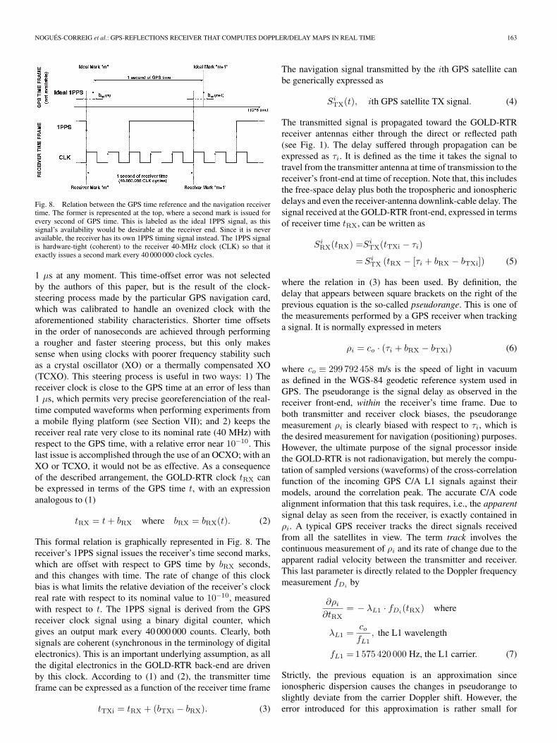
Fig. 8. Relation between the GPS time reference and the navigation receivertime. The former is represented at the top, where a second mark is issued forevery second of GPS time. This is labeled as the ideal 1PPS signal, as thissignal’s availability would be desirable at the receiver end. Since it is neveravailable, the receiver has its own 1PPS timing signal instead. The 1PPS signalis hardware-tight (coherent) to the receiver 40-MHz clock (CLK) so that itexactly issues a second mark every 40 000 000 clock cycles.

1 µs at any moment. This time-offset error was not selectedby the authors of this paper, but is the result of the clock-steering process made by the particular GPS navigation card,which was calibrated to handle an ovenized clock with theaforementioned stability characteristics. Shorter time offsetsin the order of nanoseconds are achieved through performinga rougher and faster steering process, but this only makessense when using clocks with poorer frequency stability suchas a crystal oscillator (XO) or a thermally compensated XO(TCXO). This steering process is useful in two ways: 1) Thereceiver clock is close to the GPS time at an error of less than1 µs, which permits very precise georeferenciation of the real-time computed waveforms when performing experiments froma mobile flying platform (see Section VII); and 2) keeps thereceiver real rate very close to its nominal rate (40 MHz) withrespect to the GPS time, with a relative error near 10−10. Thislast issue is accomplished through the use of an OCXO; with anXO or TCXO, it would not be as effective. As a consequenceof the described arrangement, the GOLD-RTR clock tRX canbe expressed in terms of the GPS time t, with an expressionanalogous to (1)

tRX = t+ bRX where bRX = bRX(t). (2)

This formal relation is graphically represented in Fig. 8. Thereceiver’s 1PPS signal issues the receiver’s time second marks,which are offset with respect to GPS time by bRX seconds,and this changes with time. The rate of change of this clockbias is what limits the relative deviation of the receiver’s clockreal rate with respect to its nominal value to 10−10, measuredwith respect to t. The 1PPS signal is derived from the GPSreceiver clock signal using a binary digital counter, whichgives an output mark every 40 000 000 counts. Clearly, bothsignals are coherent (synchronous in the terminology of digitalelectronics). This is an important underlying assumption, as allthe digital electronics in the GOLD-RTR back-end are drivenby this clock. According to (1) and (2), the transmitter timeframe can be expressed as a function of the receiver time frame

tTXi = tRX + (bTXi − bRX). (3)

The navigation signal transmitted by the ith GPS satellite canbe generically expressed as

SiTX(t), ith GPS satellite TX signal. (4)

The transmitted signal is propagated toward the GOLD-RTRreceiver antennas either through the direct or reflected path(see Fig. 1). The delay suffered through propagation can beexpressed as τi. It is defined as the time it takes the signal totravel from the transmitter antenna at time of transmission to thereceiver’s front-end at time of reception. Note that, this includesthe free-space delay plus both the tropospheric and ionosphericdelays and even the receiver-antenna downlink-cable delay. Thesignal received at the GOLD-RTR front-end, expressed in termsof receiver time tRX, can be written as

SiRX(tRX) =Si

TX(tTXi − τi)=Si

TX (tRX − [τi + bRX − bTXi]) (5)

where the relation in (3) has been used. By definition, thedelay that appears between square brackets on the right of theprevious equation is the so-called pseudorange. This is one ofthe measurements performed by a GPS receiver when trackinga signal. It is normally expressed in meters

ρi = co · (τi + bRX − bTXi) (6)

where co ≡ 299 792 458 m/s is the speed of light in vacuumas defined in the WGS-84 geodetic reference system used inGPS. The pseudorange is the signal delay as observed in thereceiver front-end, within the receiver’s time frame. Due toboth transmitter and receiver clock biases, the pseudorangemeasurement ρi is clearly biased with respect to τi, which isthe desired measurement for navigation (positioning) purposes.However, the ultimate purpose of the signal processor insidethe GOLD-RTR is not radionavigation, but merely the compu-tation of sampled versions (waveforms) of the cross-correlationfunction of the incoming GPS C/A L1 signals against theirmodels, around the correlation peak. The accurate C/A codealignment information that this task requires, i.e., the apparentsignal delay as seen from the receiver, is exactly contained inρi. A typical GPS receiver tracks the direct signals receivedfrom all the satellites in view. The term track involves thecontinuous measurement of ρi and its rate of change due to theapparent radial velocity between the transmitter and receiver.This last parameter is directly related to the Doppler frequencymeasurement fDi

by

∂ρi

∂tRX= − λL1 · fDi

(tRX) where

λL1 =cofL1, the L1 wavelength

fL1 =1575 420 000 Hz, the L1 carrier. (7)

Strictly, the previous equation is an approximation sinceionospheric dispersion causes the changes in pseudorange toslightly deviate from the carrier Doppler shift. However, theerror introduced for this approximation is rather small for


short-term extrapolations [see (8) below]. In GOLD-RTR, thesignals received through the up-looking antenna are continu-ously tracked by the OEM4-G2L GPS navigation receiver card.An external user can request the fDi

and ρi measurementsfrom that card through data logs. Each data log contains theaforementioned measurements for each of the GPS satellitesbeing tracked plus a time-tag indicating the moment at whichthese measurements correspond. This time-tag is expressed inthe receiver’s time frame units: tRX. This is a good match withthe purpose of having an appropriate signal model, since at thereceiver-end, everything is observed within the receiver timeframe tRX. Looking back into (5) and (6), it is clear that all thatis required to complete the model of the received signal is

1) a model of SiTX, the transmitted GPS L1 signal [33];

2) a continuous knowledge of ρi(tRX).

The signal processor achieves requirement 2) by requestingdata logs from the GPS receiver once per second. The obtainedmeasurements correspond to the 1PPS second marks, i.e., thetimes where tRX takes integer values, denoted by the integervariable m (see Fig. 8). Since the required information is notavailable continuously, but in samples at a rate of 1 Hz, atime extrapolation of the ρi(m) samples is required. This isaccomplished through Doppler integration (7). At any moment∆t after the 1PPS mark (tRX = m), the pseudorange valuescan be expressed as

ρi(m+ ∆t) = ρi(m) − λL1 ·u=m+∆t∫u=m

fDi(u) du. (8)

The preceding expression indicates that a precise knowledgeof the Doppler is necessary. Fortunately, it is available as 1-Hzmeasurements as well; once again, extrapolation is needed. Inthis case, an assumption of linear evolution is very good fora 2-s extrapolation period, since the Doppler variation in 1 s,∆fDi

(m), is in the order of 1 Hz/s, as observed from a low-dynamics (neither acrobat nor fighter) aircraft, and the secondderivative can be ignored

fDi(m+ ∆t) = fDi

(m) + [fDi(m) − fDi

(m− 1)] · ∆t= fDi

(m) + [∆fDi(m)] · ∆t. (9)

It is important to note that a 2-s extrapolation period is neededbecause microprocessor µP1 (remind Fig. 6) receives the ρi(m)and fDi

(m) measurements after the 1PPS mark m. It usesthis information to compute the signal models that will bevalid for the next second between marks m+ 1 and m+ 2.This procedure is depicted in Fig. 9. Activity A involves thecomputation of the extrapolated pseudorange ρi(m+ 1) andextrapolated Doppler fDi

(m+ 1) values by using (8) and (9).The Doppler first derivative ∆fDi

(m+ 1) is assumed to be thesame as ∆fDi

(m). Using these values, µP1 starts activity B,which involves the computation of the few signal model pa-rameters corresponding to the second between 1PPS marksm+ 1 andm+ 2.

Fig. 9. Chronogram of the steady-state procedure performed by microproces-sor µP1 in order to program the ten correlation channels with the appropriatesignal model parameters. Every time there is a receiver time second mark,asserted by the falling edge of the 1PPS signal, microprocessor µP1 waits forthe GPS satellites’ related-data burst from the GPS receiver. As soon as all thedata have been received (less than 100 ms after the 1PPS mark), µP1 startsactivity A, which consists of predicting the pseudorange, Doppler, and Dopplerrate for the next second mark m + 1, by using the previous pseudorange,Doppler, and Doppler rate measurements corresponding to mark m. With thispredicted data, µP1 starts activity B, which consists of computing the OLparameters, i.e., the signal model parameters. When complete, these are loadedinto each of the ten correlators. The correlators will use these model parametersbetween receiver marks m + 1 and m + 2 (the latter not depicted).

The signal model parameters are deduced by writingthe model of the transmitted C/A L1 GPS signal in itsanalytic form

SiTX(tTXi) = ej(2πfL1·tTXi+φ) · E(aCR · tTXi)

E(x) ≡ PRNi (x mod 1023)

PRNi(u) maps u to the ith code chip value

aCR ≡ 1.023 MHz, the C/A chipping rate (10)

where the navigation bits are not taken into account; hence,they will be present as 180 random jumps in the phase of thecomputed 1-ms waveforms every 20-ms period. The functionE(x) assumes only the value E(x) = ±1 and represents theenvelope of the signal as a periodic train of 1023 chips of thePRN spreading code of the ith GPS satellite. The function ·takes the integer part of its argument. After propagation, thetransmitted signal will be observed at the receiver-end, asindicated in (5). The analog RF front-end performs the directI and Q downconversion. This is equivalent to counterrotat-ing the received signal by the LO tone, represented by thee−j(2πFs·Mb·tRX) exponential, where Fs ≡ 40 MHz is the ref-erence clock frequency and Mb ≡ 78 756/2000 is the LO syn-thesizer multiplication factor (see Fig. 4). The reference clockfrequency has been labeled Fs because it is the sampling clockof the system, as mentioned earlier. So the BB analog I and Qreceived signal can be expressed as

SiRX(tRX) = ej

(2πfL1

(tRX− ρi(tRX)

co

)−2πFs·Mb·tRX+φ

)

·E(aCR ·

(tRX − ρi(tRX)

co

)). (11)

We shall now substitute the pseudorange with its extrapolationexpression (8) and implicitly (9) by considering the fact that westart the model with the values ρi(m+ 1), fDi

(m+ 1), and∆fDi

(m+ 1). Also, the receiver time should be substituted


with tRX = (m+ 1) + ∆t. Taking the A/D sampling at the Fs

rate into account, ∆t will take the following discrete values:

∆t ≡ n

Fs(12)

where n is the sample index starting at 1PPS mark m+ 1,ranging from 0 to 39 999 999. By adequate manipulation andchanging the integrals by summations (where du = 1/Fs), weobtain the discrete phase model, in cycles

Φ(n) = constant + C · n+D · n · (n− 1)

C ≡ fL1 + fDi(m+ 1)

Fs−Mb

D ≡ ∆fDi(m+ 1)

2 · F 2s

(13)

and the x discrete model, in chips, which is used as theargument of E(·)

x(n) = τo +A · n+B · n · (n− 1)

τo ≡(−aCR · ρi(m+ 1)

co

)

A ≡ aCR · fL1 + fDi(m+ 1)

Fs · fL1

B ≡ aCR · ∆fDi(m+ 1)

2 · F 2s · fL1

. (14)

The E(·) function, which assigns the correct chip value to itsargument x(n), is hardware implemented by merely selectingthe correct PRN code corresponding to the ith satellite to beprocessed. Regarding (13), the initial constant is unimportantsince the phase is never an absolute measurement. The digitalhardware that runs the phase model is not actually reset tozero at every 1PPS mark, but starts with the phase of the lastclock cycle before the 1PPS mark. Therefore, if a correlatoris programmed to correlate the same satellite in consecutiveseconds, the phase will not lose continuity. To summarize, whenmicroprocessor µP1 ends activity B (see Fig. 9) in accordancewith the user’s requirements, it programs each correlation chan-nel (see Fig. 7) by following three steps:

1) loads the antenna selection register with the desired value;2) loads two registers in the phase model block with theC and D values;

3) loads four registers in the envelope model block; threewith the τo,A, andB values, and a fourth register with thedesired PRN number, corresponding to the ith satellite tobe processed in that correlation channel.

At the beginning of this section, it was commented that the sig-nal phase and envelope models, as expressed in (13) and (14),would not add more than 2-mm accumulated error due to trun-cation. In the phase case, this is translated into about 1/100thof a cycle, taking into account the fact that λL1 ≡ 190.3 mm.For the x(n) function case, as it is expressed in chips, this istranslated into 1/150 000th of a chip since 1 chip = 300 m.

Since n takes values from 0 to 39 999 999, this is translated intothe following precision requirements:

1) τo: (chips): 2−20;2) A: (chips/sample): 2−44;3) B: (chips/sample2): 2−68;4) C: (cycles/sample): 2−32;5) D: (cycles/sample2): 2−57.

The digital hardware that runs automatically in each correlationchannel, the phase and envelope models, has been implementedwith the above binary precisions. Up to now, it has beenassumed that the OEM4-G2L GPS receiver inside the GOLD-RTR delivered the correct ρi and fDi

measurements for allthe satellites in view; this is only true for the signals receivedthrough the direct ray, which are the only ones tracked by theGPS receiver, but not for the reflected ones (see Fig. 1). In thislatter case, the signal processor assumes a simple geometricmodel that describes the additional propagation delay experi-enced by the reflected signal with respect to the direct one

∆ρi = 2 · (H − U) · sin(e). (15)

This simple model is accurate enough when flying in a vehicleat a low height above the geoid, in comparison with the radius ofthe Earth. H represents the height of the vehicle above the ref-erence ellipsoid, as provided in real time by the GPS navigationreceiver card, while U represents a user specified undulation,which is useful should the reflecting surface would not be at thereference ellipsoid level; e represents the GPS satellite’s eleva-tion as observed with respect to the local horizon, also providedby the GPS receiver in real time. In this situation, the sea surfaceis seen locally as a flat surface. It has also been assumed thatthe vehicle velocity vector is parallel to that surface, so that theDoppler of the specular point of the reflected signal is the sameas the direct one. Therefore, when computing open-loop signalmodels for the reflected signals, the signal processor uses thesame Doppler as for the direct signal,1 and adds the additional(15) quantity to the direct signal’s pseudorange measurement.

C. Correlators Schedule

The signal processor does not have any decision-making ca-pacity in order to avoid uncontrolled actions. It programs eachcorrelation channel exactly as the user requires. This is accom-plished by means of a configuration file, which the user loadsonto the signal processor via Ethernet by means of the graphicaluser interface (GUI) running on the laptop. The configurationfile is a series of configuration lines. Each configuration linecontains the following information:

1) a time-tag indicating the GPS week and second of theweek at which the configuration line is first valid;

2) the following parameters repeated ten times to accountfor each of the ten correlation channels.a) The run/idle flag, indicating whether the correlation

channels have to be programmed or not. If idle, thesignal processor does not send waveforms to thelaptop.

1However, if the user forces an offset in the Doppler (see Section IV-C), then,this is added to the Doppler estimate in open-loop signal models.


b) The PRN number of the GPS satellite to be processed.May range from 1 to 32 for normal GPS satellites,and as well as codes from 120 to 139 for GPS-WAASsatellites.

c) The antenna link number that selects the GOLD-RTR antenna input used as a source signal for crosscorrelation. It ranges from 1 to 3.

d) The up/down flag, indicating whether the model to beapplied is up or down, as explained earlier (15).

e) The delta frequency offset, ranging from −511 to512 Hz, to force an offset in the Doppler. This directlyaffects parameters C and A of the open-loop envelopeand phase signal models in (13) and (14).

f) The delta delay offset, ranging from −1023 to 1024m, to force an offset in the default pseudorange model.This directly affects parameter τ0 of the open-loopenvelope signal model in (14).

g) The undulation, to consider the height of the reflectingsurface with respect to the reference ellipsoid (15).

Not all combinations of the previous parameters are accepted.Particularly, the time-tags of each line must be consecutive,with a minimum separation of 1 s. Therefore, the correlators’configuration can be changed as often as once per second.Another restriction is the fact that, if a correlator is programmedwith antenna link one selected, the up/down flag must be set toup since that antenna should always be up-looking. Flexibilityis accounted for in the remaining parameter combinations. Sec-tion VII depicts some of these combinations. The preparation ofa configuration file for an experiment requires prior knowledgeof the following.

1) The precise time the experiment is going to start and stop.2) Through what geographical points the instrument is going

to move during the experiment, so as to order the signalprocessor to process the correct satellites. Should a cor-relator be programmed with a satellite that is not beingtracked by the GPS receiver, the computed waveformswould be marked as satellite not available.

When the signal processor is loaded with a configuration file, italways compares its own time with the configuration file time-tags. If the time-tag of the first line of the file is for a time afterthe present moment, the signal processor waits until that mo-ment. If it marks a time before the present, the signal processormoves its task pointer between lines, with time-tags indicatingmoments before and after the present moment. In whatevercase, when the GPS time reaches the time-tag correspondingto each line, the signal processor programs (1 s in advance) thecorrelators with the user required configurations. Furthermore,it continues to program the correlators with such configurationsuntil the GPS time reaches the time-tag of the next line.

D. Waveforms Data Format

If the signal processor is loaded with a configuration file, itwill dump a set of ten data structures in every millisecond, eachcontaining the 64-lag 1-ms waveform that was computed in realtime in each correlation channel, plus additional data indicatingthe relevant correlation model parameters used and status flags.A C-expression describing this structure is depicted in Fig. 10.

Fig. 10. Waveform data structure declaration in C language. Those variablespreceded by the mnemonic char use 1 B, those preceded by short use 2 B,and those preceded by int use 4 B. The structure begins with 32 B carryingseveral additional data parameters, and ends with an array of 128 characterscarrying the 64 I and Q pairs of a 1-ms waveform, computed within a correlator(see Fig. 7).

The structure has 160 bytes. Those variables preceded by themnemonic char use one byte, those preceded by short usetwo bytes, and those preceded by int use four bytes. The32 leading bytes form a header carrying the additional data,while the DATA[128] character array carries the 64 lags corre-sponding to the 1-ms real-time computed waveform. Each lag isan I andQ pair, one byte for I and one byte forQ, respectively,codified in two’s complement. The parameters in the headerhave the following meanings.

1) WEEKSOW and MILLISECOND is a time-tag, expressed inreceiver time tRX, of the moment at which the signalprocessor began to compute the waveform. For geo-referenciation purposes it can be considered as GPS time,since the receiver time offset is always smaller than 1 µs.

2) STATUS_NUMCORR indicates at what correlation channelthe waveform was computed (1–10) and the status of thewaveform. Status can be OK, navigation bit, and satellitenot available. The first indicates that the data are correct.The second indicates that data are correct but there couldbe a jump of 180 in the phase during that millisecond,due to the navigation data modulation impinged in thenavigation signal; it is better to ignore waveforms markedas such because this only happens once every 20 ms forGPS normal satellites (1–32). The last possible statusindicates that the requested satellite to be processed wasnot tracked by the GPS receiver, so the waveform data isonly noise.

3) LINK_UPDW indicates what antenna link (1–3) was usedas a signal source for cross correlation and whether themodel used was for direct signals (up) or for reflectedsignals (down), as explained in Section IV-B.

4) PRN is the PRN number of the processed satellite.5) MAX_POS is the index of the waveform lag with

greatest power.6) AMPLITUDE of the waveform at the MAX_POS lag.7) PHASE is the phase of the waveform at the MAX_POS lag.


8) RANGE_MODEL is zero if the model was up and takes thevalue indicated in (15) if the model was down.

9) DOPPLER_UP is the fDiDoppler value delivered by the

navigation receiver, corresponding to the direct signal ofthe indicated PRN number. This value, plus the D_FREQvalue (see below) is the Doppler estimation used forcrosscorrelation for both the up or down signals. This di-rectly affects parameters C and A of the open-loop signalmodel [(13) and (14)].

10) SAMPLING_FREQ_INT and SAMPLING_FREQ_FRAC de-scribe the sampling frequency (integer and fractionalpart), measured between 1PPS marks. This parameteris only kept for backward compatibility with previousversions of GOLD-RTR. This parameter always containsthe 40 000 000 value, and the fraction is zero.

11) D_FREQ Doppler offset that was forced by the user andadded to the Doppler frequency. This directly affectsparameters C and A of the open-loop signal model [(13)and (14)].

12) D_DELAY delay offset forced by the user, that was addedto the pseudorange. This directly affects parameter τ0 ofthe open-loop signal model (14).

13) SIN_ELEVATION the sine of the satellite’s elevation asseen on the local horizon.

When the GOLD-RTR is working, it dumps a stream of1 600 000 bytes/s through the Ethernet. This flow is sinked bythe laptop, which stores the real-time computed waveforms inseveral files. The total amount of data that can be stored islimited only by the capacity of the laptop’s hard disk drive.

V. MACHINE–USER INTERFACE

The GOLD-RTR instrument is controlled through a GUIrunning on the laptop. A screen shot of this application is shownin Fig. 11. The GUI provides the following.

1) The GOLD-RTR status is a blinking text label to providea way of monitoring the health of the instrument, indicat-ing whether the instrument status flags are continuouslyreceived via Ethernet or not.

2) GPS satellite availability to show the PRN number aswell as the received C/No for all the GPS satellitestracked by the GPS receiver. The GPS time and date arealso displayed.

3) User action buttons, divided between test and experimentactions. In both cases, the configuration button indicatesthe directory where the waveform data has to be storedand the path of the configuration file containing thecorrelation actions indicated by the user. The test actionautomatically performs a test, which consists of an au-tomatically generated experiment of several seconds forchecking purposes. The results are graphically displayedat the end of the test. The start action loads the instrumentwith the user-specified configuration file. The button thenchanges its label to stop, so that the user can abort theexperiment before the scheduled time.

4) The log register provides logs of user actions as well asautomatic actions performed by the GUI.

Fig. 11. Screen shot of the GOLD-RTR GUI, running on the laptop (seeFig. 2). The interface provides: 1) status of the GOLD-RTR (top left);2) availability of GPS satellites (top center); 3) instrument controls (top right);4) actions log register (bottom); and 5) real-time altimetric application graph(above the log register).

5) The altimetric application graph is a real-time applicationthat uses GPS-R signals to determine the height of theup-/down-looking pair of antennas with respect to thereflective surface.

VI. LABORATORY READINESS TESTS

In order to check the correctness of the signal modelsgenerated by the signal processor (see Section IV-B), a con-trolled laboratory test was performed, in which there wasstrong knowledge of the signals gathered by the GOLD-RTRinstrument. This was accomplished by using a SPIRENT GPSsimulator test-bench. This comprised an NTNE10BA version(L1 only) STR4760 signal generator hardware platform andthe SimGEN software running on a personal computer. Thissimulator provides an RF output signal that contains the sameL1 GPS signals that would be observed in the output port ofa receiving GPS antenna, as if moving in the real scenariobeing simulated. The STR4760 hardware platform provides away of generating such a signal mixture, while the SimGENsoftware performs all the calculations to run the simulationand controls the STR4760 in order to generate the GPS signalsaccordingly. In order to emulate a real scenario with a static po-sition, SimGEN only requires the corresponding GPS satellites’constellation almanac data in YUMA format, and the x–y–zECEF coordinates of the antenna position. The test was de-signed to reproduce the true-scenario conditions in which wave-form data had been experimentally collected beforehand withthe GOLD-RTR instrument. The experiment was conducted on41.4 N, 2.1 E, about 300 m above mean sea level, and datawere recorded on March 23, 2005, beginning at 15 h, 23 m, and0 s. The site was on the top of a hill, with full visibility of the


Fig. 12. Comparison of waveforms for satellite PRN 24 obtained in (top) areal field scenario and the same waveforms obtained when the GOLD-RTR wasworking under (bottom) a SPIRENT GPS simulator test bench that emulatesthat scenario. The signals gathered in the real scenario were uncontrolled,always in the presence of multipath, while the signals gathered in the GPSSPIRENT test bench were totally controlled, without multipath. Each graphdepicts 120 s of 1-s integrated waveforms and the residuals of these waveformsafter subtracting the best-fit of its model around the peak.

whole zenith hemisphere, with no nearby metallic structures.A zenith-pointing choke-ring antenna was used. Despite of allthese multipath-avoidance precautions and after 1-s integration(50 dB SNR), the collected waveforms still seemed to indicatethe presence of a diffuse multipath, comparable to thermal noisepower levels (see Fig. 12, real scenario). Since this was a veryslight effect, doubts may have arisen about their true origin:real multipath or mismodeling errors in the cross-correlationsignal models. If it was a mismodeling error, this has to appearin the simulated environment as well. If it was real multipath,the waveforms collected in the simulated environment shouldnot show evidence of the described effects and should exactlymatch the corresponding PRN code autocorrelation, only cor-rupted by the presence of thermal noise. The laboratory testwas performed on May 27, 2005. The STR4760 RF outputwas plugged to the GOLD-RTR up-looking antenna input. It

was loaded with the same configuration file as that used in thereal scenario. This configuration file had only one line, withinstructions for programming eight of the ten correlators to col-lect waveforms corresponding to the eight satellites that were inview on March 23, at that particular site. The test lasted 120 s,obtaining a total of 120 000 1-ms coherent integrated wave-forms for every satellite. For both the real and simulated scenar-ios, the 120 s of real-time-collected data was further integratedup to 1-s periods, reducing the results to just 120 waveformsper satellite. A comparison of the results for both the real andsimulated scenarios and for just one of the eight processedsatellites is shown in Fig. 12. There are two graphs for eachscenario. The top graph shows the 120 superimposed 1-sintegrated waveforms. Only the I component is shown sincethe waveforms have been counterrotated toward the real axis.This process is necessary in order to correctly compare thereal cross correlation with the theoretical infinite-bandwidthPRN code autocorrelation. The residuals graph is shown belowthe waveforms graph, depicting the superimposed differencesbetween each waveform and its best-fit model. The model usedis the exact theoretical PRN autocorrelation of that particularsatellite. The delay fitting is performed by implementing anearly prompt-late delay discriminator with three lags aroundthe peak. The estimation of amplitude is taken to be that corre-sponding to the lag with the greatest power. The simulated sce-nario waveform data in Fig. 12 show that the 120 superimposed1-s waveforms are structured evenly left to right with respectto the peak; the background noise rms power seems even. Thisis confirmed in the residuals, which show this even symmetrybetter. At the center of the residuals graph, the thermal noiseis nearly zero because the method for estimating the time ofarrival (TOA) works around the central lag. The noise power in-creases gradually from the center up to the edges of the triangledue to its autocorrelation statistics. These simulated-scenarioresults match the theoretical predictions, thus confirming thatthe signal models used in the signal processor are adequate.This confirms that the unevenness of the residuals in the realscenario is the result of diffuse multipath. In this latter case,the increase in the power of the residuals toward the right is aconfirmation that a small fraction of back-scattered energy fromthe surrounding terrain was received with an additional delay.

VII. FIRST FLIGHT CAMPAIGNS

Two successful flights using a pressurized jet aircraft wereperformed on July 13 and 14, 2005, at ∼9300 m above meansea level and ∼130-m/s speed, flying over two different areasof the western Mediterranean. A total amount of 5 h of real-time data was collected, which corresponds to 180 million 1-mswaveforms (29 GB). The purpose of the flights was to checkthe instrument’s performance for altimetric, scatterometric, andpolarimetric applications. This was accomplished by loadingthe GOLD-RTR with several configuration files, which wereconsecutively loaded into the instrument during the flights by anonboard human operator. These files were prepared beforehandto test all the useful combinations with the parameters thatcontrol the cross-correlation models in each of the ten corre-lation channels: up or down, signal source link (1–3), forced


Fig. 13. (Left) Direct and (right) reflected 64-lags amplitude waveforms corresponding to PRN 27 1 s of integration time. The signal power was normalized tothe background Gaussian noise power, so that the amplitude is expressed in SNR voltage units. The SNR peaks are 50.5 and 34.5 dB, respectively. Note that, thereflected waveform appears quite undistorted; this is because the sea was not too rough in the observed zone.

delay-offset, and forced Doppler-offset. This section providessamples of the real-time collected waveforms, which graphi-cally illustrate some of the combinations tested, a sample ofthe real-time GNSS-R altimeter application that may be rununder the GOLD-RTR GUI (see Section V) and preliminarymeasurements of the sea roughness.

A. Direct/Reflected Delay Maps

These measurements are obtained by using two correlationchannels per PRN code, one for the up-looking right-hand cir-cularly polarized (RHCP) antenna and the other for the down-looking left-hand circularly polarized (LHCP) antenna, up tofive PRNs simultaneously. Therefore, the instrument computesand stores in the laptop disk ten complex-valued 1-ms wave-forms per millisecond. Upon postprocessing, these waveformsare further integrated up to 1 s in order to achieve a higher SNR.A sample pair of direct/reflected 1-s waveforms is shown inFig. 13. Since the signal models used in the real-time cross-correlation process are valid and accurate enough for periods of1 s (see Section IV-B), the integration of the 1-ms waveformsup to 1-s periods does not require any time realignment of the1-ms waveform lags prior to further postprocessing integration.The latter consists of the following.

1) The coherent summations of ten 1-ms waveforms (directsummation of complex-valued waveforms), which resultsin 10-ms coherent waveforms. The corresponding band-width for these 10-ms waveforms is 100 Hz.

2) The incoherent summation of 100 10-ms waveforms.This is accomplished by: 1) counterrotating each 10-mswaveform with the phase of the lag of greatest power andthen taking only the real part of the resulting waveformand 2) performing a direct summation of the 100 real-valued resulting waveforms. This approach only worksif the SNR at 10 ms is around 6 dB or greater, so that

the signal phase is properly estimated. But, it has theadvantage that: 1) the resulting 1-s waveforms are cor-rupted only by Gaussian zero-mean noise statistics and2) the waveform shape can be directly compared to thecorresponding theoretical PRN code autocorrelation.

This approach opens the possibility of a linear resolution ofthe problem, i.e., trying to identify the sea reflection channelby comparing the direct and reflected waveforms, as a clas-sical linear channel identification problem corrupted by zero-mean Gaussian noise. Note that, this would not be possiblein the traditional incoherent integration method, which takesthe square root of the power of each waveform lag, yielding:1) a Rice nonzero-mean noise statistics that is parameterized bythe signal’s amplitude; and 2) a waveform shape that cannotbe directly compared to the theoretical PRN autocorrelationbecause it has been distorted when taking the square root ofeach lag’s power. The data acquired using this configurationshowed that the reflected waveforms are correctly aligned withthe direct ones according to the range model provided by thenavigation card. This is a useful result since it indicates thatthe reflected-to-direct delay of the signals can be identicallyobtained with sole measurements of the reflected waveformsplus the RANGE_MODEL parameter (see Section IV-D) applied inthe signal processor, with no need to occupy correlation chan-nels to allocate the waveforms of the direct signals. Therefore,the GOLD-RTR is able to acquire altimetric data for up to tensatellites in parallel.

B. Doppler/Delay Maps

These measurements are obtained by using all the correlationchannels with a single PRN code. We devoted the first channelto cross-correlate against the direct signal coming from the up-looking antenna (not necessary any more as discovered afterthe experiment and explained above), while the remaining nine


Fig. 14. Doppler/delay amplitude map (9 × 64 bins), corresponding to 1 sof data. The grayscalebar units are expressed in SNR voltage. This map hasbeen computed by coherently integrating the 1-ms waveform products upto 10 ms and then incoherently integrating—by taking the square root ofthe power—up to 1 s. These observations were obtained by configuring theinstrument with nine correlation channels cross correlating against the reflectedsignals and forcing Doppler offsets in the counterrotation phasor model from−200 to 200 Hz, in 50-Hz steps.

channels cross correlated against the reflected signals by forc-ing different frequency offsets in the signal model (D_FREQ inSection IV-D). A range of frequencies from −200 to 200 Hz, in50-Hz steps, were selected. The further integration of the 1-mswaveforms is coherent up to 10 ms (then the bandwidth is100 Hz) and incoherent up to 1 s. The incoherent integration ismade by taking the square root of the power of each waveformlag (the classical method). The result is one Doppler/delaypower map per second of the reflected signal data. A sample ofsuch a map is shown in Fig. 14 as a grayscale-filled contour plot.The amplitude is expressed in SNR voltage after 1-s integration.

It is important to note that the roughly half-moon shape of themap matches the theoretical predictions: the energy reflectedoff the specular reflection point has the least delay and zeroDoppler. As we move away from the specular reflection point,the scattered signal is always affected by an additional Doppler,and the propagation path is greater, providing an additionaldelay. Such a map can be used to sense the characteristics ofthe reflecting surface roughness and, indirectly, surface windspeed vectors (e.g., [53]).

C. Real-Time Coarse Altimetric Application

The GOLD-RTR instrument features a real-time coarse alti-metric application that runs in parallel with the waveform stor-age application in the laptop. The altimetric application onlyruns if the GOLD-RTR has already been loaded through thedemo or test actions buttons (see Fig. 11), with a configurationfile that groups the ten correlation channels into five up/downpairs, each pair correlating against a single PRN (note that,from the results of the experimental data shown afterward, it isalso possible to use the ten correlator channels to pick re-flected signals, since the waveforms obtained are aligned ac-

cordingly to the known range model). Under these conditions,the altimetric application receives five up/down waveform pairsevery millisecond. The application further integrates these 1-mswaveforms up to one second, yielding five high-SNR up/downwaveform pairs. An example of such a waveform pair is shownin Fig. 13. Using this information, it computes five delayobservables every second, i.e., the differences in TOA betweenthe direct and reflected signals. This computation is made usingan early-prompt-late estimator, with the underlying assumptionthat the reflected signal will be of the same shape as the directone. Strictly, this is only true at very low altitudes or when thereflecting surface is almost flat.2

The following simple model is used in this application torelate the five delay observables ∆ρi with the aircraft heightabove sea level

∆ρi = 2 · (HMSL) · sin(e) + bc. (16)

The model has only two parameters: the aircraft height abovemean sea level HMSL and a constant bias bc. This bias absorbsboth the difference in the downlink-cable lengths betweenthe down- and up-looking antennas, and the difference in theD_DELAY parameter set by the user between the down andup waveforms (see Section IV-D). The sine of the satelliteelevation e above the local horizon is recorded in the waveformheader (once again see Section IV-D). The estimation of theHMSL and bc parameters is made by performing a simple leastsquares fit of the model to the five delay observables. The resultis a measurement of the aircraft height above sea level everysecond. The two flights performed on July 13 and 14 weremainly programmed for collecting scientific data. This was ac-complished for almost all the time that the aircraft was flying atthe same height. However, both the climb and descent phases ofthe flights were free. So, we took the opportunity in both flightsto perform a coarse real-time altimetric test at the end of theflight during the descent. Graphical results corresponding theJuly 14 test are shown in Fig. 15. Only about 3 min is shown inorder to clarify the precision of this GNSS-R passive real-timeaircraft RADAR altimeter. In the top panel, the GNSS-R real-time aircraft height measurements (dots) are compared with:1) the precise trajectory (solid line) of the aircraft and 2) thereal-time height measurements provided by the Novatel OEM4-G2L GPS receiver card (dashed line). The precise trajectory ofthe aircraft is computed by the GPS standard fine postprocess,using the observables generated onboard by the GPS receivercard, and the precise a posteriori satellite orbits and clocks.This is considered the true trajectory. It should be noted thatGPS-R measurements are single frequency (L1) and differen-tial, while both the real-time and postprocess GPS positioningare dual frequency (L1 and L2) and absolute. In the bottompanel, a ground projection of the aircraft’s trajectory is shown(solid line) during the mentioned descent phase and landingas well as the ground tracks of the specular reflection points(gray spots) of the GPS-R signals processed by the GNSS-Rreal-time coarse altimeter. The precision of the GNSS-R real-time height measurements is shown to be about 4-m rms before

2However, this application was only designed for demonstration purposes.


Fig. 15. (Top) Aircraft height measurements with respect to the sea surface,corresponding to the final descent phase and landing of the July 14, 2005flight. The real-time coarse GNSS-R height measurements (dots) are comparedwith: 1) the precise trajectory (solid line) computed by the GPS standard finepostprocess methods, using the precise GPS satellite orbits and clocks and2) the real-time height measurements provided by the Novatel OEM4-G2LGPS receiver card (dashed line). (Bottom) Ground projection of the aircraft’strajectory over the background image of the city of Barcelona during theaforementioned descent phase (solid line) and ground tracks of the specular re-flection points (gray spots) of the GPS-R signals processed. Barcelona LandsatTM background image: ESA Copyright 2004. Distributed by Eurimage.

approaching point (A). This may be fairly coarse, but does how-ever reasonably match the fact that, when using an Earth-boundomnidirectional GPS antenna for standard GPS positioning, the

accuracy of the envelope-based3 pseudorange observables after1 s of integration (and using an early prompt-late estimator) isabout 1 m rms. [54]. Apart from the direct signals, the altimet-ric application also deals with reflected signals. The reflectedsignals are affected by factors that degrade the SNR, such asthe sea surface reflection coefficient (lower than one) and thesea surface roughness which distorts the signal shape. Thiseffect worsens as altitude increases, introducing greater offsetsin the determination of the reflected signal’s delay. From point(A), the noise in the GNSS-R height measurements increasesabruptly. This is probably due to the transition from sea toground, where reflections may come from multiple directionsand signal strength is reduced. Point (B) marks a short sequenceof about 5 s, very near to the ground, where noise is reducedback again to the 4 m rms. During this phase, the aircraft flewover a natural protected zone that has a pond. Point (C) marksthe landing time/place. This passive GNSS-R altimeter could beuseful as an alternative to standard real-time GPS positioning,when used only for purposes of height determination. It hasto be noted that the accuracy of real-time GPS positioning isaffected by the precision of the real-time broadcast satelliteephemerides, which can induce position biases in the order oftens of meters. The dashed line in Fig. 15 is biased with respectto the solid line. The GNSS-R real-time altimeter presentedhere is independent of this (because it is differential) and couldeasily provide unbiased height measurements when flying atlow altitudes.

D. Near-Real-Time Sea Surface Roughness

A set of algorithms has been designed and implementedfor inverting delay waveforms into sea-surface-roughness es-timates in a near-real-time pipe. Because of the low computingcosts and the independence of this approach from postprocessedGPS products (such as precise orbits, transmitter clock correc-tions, or receiver trajectory), this algorithm could be integratedin the software part of the instrument to provide the mean-square slopes (MSS) of the sea surface. The technique isbased on the nonlinear relationship between the supplementarydelay suffered by the reflected waveform (shifting its peaklocation with respect to the optical reflected path delay) andthe sea surface roughness statistics. In the past [6], a simplifiedmodel was used to relate the roughness driven delay and theeffective (calibration requiring) MSS product. The approachhas now been enhanced by using a complete integral model(absolute, no need of calibration) such as the one in [23],using the sea surface spectrum of [20]. The combined modelprovides the power waveform as a function of the geometricparameters and the surface MSS: P mod (τ ; geometry,mss).The same peak-extractor operator used on the real data isused here to interpolate the delay of the maximum ampli-tude of the modeled waveform: ∆ρmodel

scatt (mss, geometry) =PeakExtract[P mod (τ ; geometry,mss)]. The partial derivativeswith respect to an a priori value of the mss (mss0) are finallyused to linearize the model: [∆ρmodel

scatt (mss)−∆ρmodelscatt (mss0)]/

[mss − mss0]. The iteration number depends on the quality ofmss0. We applied this technique to the data obtained during the

3Not smoothed by the carrier phase


Fig. 16. (Top) MSS obtained with the near-real-time application and averagedat ∼3-km along-track resolution. The color scale stands for the time, in hoursof the day (UTC). A clear north–south gradient of the surface roughnessis detected, and some of its finer features are consistent along the repeatedsubsequent over passes. Moreover, the gradient is consistent with the windspeed reanalyzed by ECMWF (background color in bottom figure), where wehave over plotted the trajectory of the craft (red line).

July 2005 flights. The resulting MSS, averaged within ∼3-kmalong-track resolution, is displayed in Fig. 16 (top) while theaircraft flew six times over an ∼100-km straight path for 2 h[Fig. 16 (bottom)]. The dispersion of the averaging process issmall (< 0.001 on average), allowing the detection of featuresbelow a 10-km horizontal scale that are consistent along thedifferent subsequent over passes. Furthermore, a north–southgradient of the MSS is identified, in qualitative agreementwith the ECMWF reanalyzed wind product [Fig. 16 (bottom)].Therefore, the GOLD-RTR potentially becomes a near-real-time instrument for providing L-band MSS of the sea surface.

VIII. SUMMARY

A technical description of the GOLD-RTR receiver has beenpresented, covering the hardware architecture and user interfaceof the instrument, its internal signal-processor architecture,and its signal-processing chain. All the relevant details havebeen explained for automatic real-time computation through tenindependent correlation channels, each millisecond, of 64-lagcomplex-valued cross correlations between the input L1 C/AGPS signals and their models. The observations that can be

made with the GOLD-RTR receiver are highly flexible, makingit possible to compute several synchronous delay maps foraltimetry applications or Doppler/delay maps for scatterome-try/polarimetric applications. The review of the instrumentationused previously in the field of Earth remote sensing usingGPS-R clearly shows that the GOLD-RTR receiver provides anew and highly appropriate framework for the scientific user,who is mainly interested in extracting geophysical informationfrom the waveforms, but not in computing the waveforms them-selves. The GOLD-RTR provides a huge amount (comparedto previous instruments) of automatically real-time computedwaveforms immediately after an experiment, appropriatelyrecorded in data structures, without the need of any effortfrom the user. The aim of the present paper is to provide anappropriate comfortable framework for the GPS-R communityto perform thorough field campaigns and to noticeably speed upthe study of GPS-R remote sensing techniques.

ACKNOWLEDGMENT

The authors would like to thank J. T. Badia and S. R. Vedrillafor their contributions in the assembly of the GOLD-RTRinstrument hardware as well as their participation in the July2005 flights, D. Pino (IEEC/UPC) for extracting the ECMWFproducts, The Centre Tecnològic de Telecomunicacions deCatalunya (CTTC) for providing access to their RF instrumen-tation several times during the development phase of the instru-ment, J. Torres and J. R. M. Romero from the Instituto Nacionalde Técnica Aeroespacial (INTA) for facilitating the use of theirSPIRENT GPS simulator, The Institut Cartogràfic de Catalunya(ICC) for computing the aircraft kinematic solutions and theirpilots (Santi and Jordi) for the careful execution of the flightplans, and A. Hirschmann and D. Owen for checking the styleof the manuscript.

REFERENCES

[1] R. A. Simpson, “Spacecraft studies of planetary surfaces using bistaticradar,” IEEE Trans. Geosci. Remote Sens., vol. 31, no. 2, pp. 465–482,Mar. 1993.

[2] M. Martín-Neira, “A passive reflectometry and interferometry system(PARIS): Application to ocean altimetry,” ESA J., vol. 17, pp. 331–355,Dec. 1993.

[3] M. Martín-Neira, M. Caparrini, J. Font-Rosselló, S. Lannelongue, andC. S. Vallmitjana, “The PARIS concept: An experimental demonstrationof sea surface altimetry using GPS reflected signals,” IEEE Trans. Geosci.Remote Sens., vol. 39, no. 1, pp. 142–149, Jan. 2001.

[4] J. L. Garrison, S. J. Katzberg, and C. T. Howell, “Detection of oceanreflected GPS signals: Theory and experiment,” in Proc. IEEE Southest-con Engineering the New Century, Blacksburg, VA, Apr. 12–14, 1997,pp. 290–294.

[5] S. T. Lowe, C. Zuffada, Y. Chao, P. Kroger, L. E. Young, andJ. L. LaBrecque, “5-cm precision aircraft ocean altimetry using GPSreflections,” Geophys. Res. Lett., vol. 29, no. 10, 1375, May 2002.

[6] A. Rius, J. M. Aparicio, E. Cardellach, M. Martín-Neira, and B. Chapron,“Sea surface state measured using GPS reflected signals,” Geophys. Res.Lett., vol. 29, no. 23, 2122, Dec. 2002.

[7] G. Ruffini, F. Soulat, M. Caparrini, O. Germain, and M. Martín-Neira,“The Eddy experiment: Accurate GNSS-R ocean altimetry from low alti-tude aircraft,” Geophys. Res. Lett., vol. 31, no. 12, L12306, Jun. 2004.

[8] K. Anderson, “A global positioning system (GPS) tide gauge,” NATOAdvisory Group for Aerosp. Res. Develop., Tech. Rep. CP-582, 1996.

[9] R. N. Treuhaft, S. T. Lowe, C. Zuffada, and Y. Chao, “Two-cmGPS altimetry over Crater Lake,” Geophys. Res. Lett., vol. 28, no. 23,pp. 4343–4346, 2001.


[10] M. Belmonte and M. Martín-Neira, “GNSS reflections: First altimetryproducts from bridge-2 field campaign,” in Proc. 1st ESA Workshop Satel-lite Navigat. User Equipment Technol. (NAVITEC), 2001, pp. 465–479.

[11] M. Martín-Neira, P. Colmenarejo, G. Ruffini, and C. Serra, “Altimetryprecision of 1 cm over a pond using the wide-lane carrier phase of GPSreflected signals,” Can. J. Remote Sens., vol. 28, no. 3, pp. 394–403,Jun. 2002.

[12] M. L. Beekhuis, M. Belmonte, N. Bastarrachea, M. Martín-Neira,J. Torrobella, and O. Nogués-Correig, “Zeelandbrug III experiment, aGPS-R experiment with new GNSS-R receiver to retrieve geophysicalparameters as sea surface roughness and sea level,” in Proc. Oceanog-raphy with GNSS Reflections Workshop, Jul. 17–18, 2003, pp. 111–112.[Online]. Available: http://starlab.es

[13] M. Caparrini, L. Ruffini, and G. Ruffini, “PARFAIT: GNSS-R coastalaltimetry,” in Proc. Workshop Oceanography with GNSS Reflections,Jul. 17–18, 2003, pp. 51–68.

[14] E. Cardellach, C. O. Ao, M. de la Torre-Juárez, and G. A. Hajj, “Car-rier phase delay altimetry with GPS-reflection/occultation interferometryfrom low Earth orbiters,” Geophys. Res. Lett., vol. 31, no. 10, L10402,May 2004.

[15] J. L. Garrison and S. J. Katzberg, “The application of reflected GPSsignals to ocean remote sensing,” Remote Sens. Environ., vol. 73, no. 2,pp. 175–187, Aug. 2000.

[16] A. Komjathy, V. U. Zavorotny, P. Axelrad, G. H. Born, and J. L.Garrison, “GPS signal scattering from sea surface: Wind-speed retrievalusing experimental data and theoretical model,” Remote Sens. Environ.,vol. 73, no. 2, pp. 162–174, Aug. 2000.

[17] J. L. Garrison, A. Komjathy, V. U. Zavorotny, and S. J. Katzberg, “Windspeed measurement using forward scattered GPS signals,” IEEE Trans.Geosci. Remote Sens., vol. 40, no. 1, pp. 50–65, Jan. 2002.

[18] E. Cardellach, G. Ruffini, D. Pino, A. Rius, A. Komjathy, and L. Garrison,“Mediterranean balloon experiment: Ocean wind speed sensing from thestratosphere using GPS reflections,” Remote Sens. Environ., vol. 88, no. 3,pp. 351–362, Dec. 2003.

[19] O. Germain, G. Ruffini, F. Soulat, M. Caparrini, B. Chapron, andP. Silvestrin, “Speculometry from low altitude aircraft,” in Proc. Oceanog-raphy with GNSS Reflections Workshop, Jul. 17–18, 2003, pp. 107–110.[Online]. Available: http://starlab.es

[20] T. Elfouhaily, B. Chapron, K. Katsaros, and D. Vandemark, “A unifieddirectional spectrum for long and short wind-driven waves,” J. Geophys.Res., vol. 102, no. C7, pp. 15781–15796, Jul. 1997.

[21] J. L. Garrison, S. J. Katzberg, and M. I. Hill, “Effect of sea rough-ness on bistatically scattered range coded signals from the global po-sitioning system,” Geophys. Res. Lett., vol. 25, no. 13, pp. 2257–2260,Jul. 1998.

[22] B. Lin, S. J. Katzberg, J. L. Garrison, and B. A. Wielicki, “Relation-ship between GPS signals reflected from sea surfaces and surface winds:Modeling results and comparisons with aircraft measurements,” J. Geo-phys. Res., vol. 104, no. C9, pp. 20 713–20 727, Sep. 1999.

[23] V. U. Zavorotny and A. G. Voronovich, “Scattering of GPS signals fromthe ocean with wind remote sensing application,” IEEE Trans. Geosci.Remote Sens., vol. 38, no. 2, pp. 951–964, Mar. 2000.

[24] T. Elfouhaily, D. R. Thomson, and L. Linstrom, “Delay-doppler analysisof bistatically reflected signals from the ocean surface: Theory and appli-cation,” IEEE Trans. Geosci. Remote Sens., vol. 40, no. 3, pp. 560–573,Mar. 2002.

[25] C. Zuffada, A. Fung, J. Parker, M. Okolicanyi, and E. Huang, “Po-larization properties of the GPS signal scattered off a wind-drivenocean,” IEEE Trans. Antennas Propag., vol. 52, no. 1, pp. 172–188,Jan. 2004.

[26] D. Masters, V. U. Zavorotny, S. J. Katzberg, and W. Emery, “GPS signalscattering from land for moisture content determination,” in Proc. IEEEIGARSS, Honolulu, HI, Jul. 24–28, 2000, pp. 3090–3092.

[27] A. Komjathy, J. Maslanik, V. U. Zavorotny, P. Axelrad, and S. J. Katzberg,“Sea ice remote sensing using surface reflected GPS signals,” in Proc.IGARSS, Honolulu, HI, Jul. 24–28, 2000, pp. 2855–2857.

[28] S. T. Lowe, J. L. LaBrecque, C. Zuffada, L. J. Romans, L. E. Young,and G. A. Hajj, “First spaceborne observation of an Earth-reflected GPSsignal,” Radio Sci., vol. 37, no. 1, pp. 7-1–7-28, Feb. 2002.

[29] G. Beyerle and K. Hocke, “Observation and simulation of direct andreflected GPS signals in radio occultation experiments,” Geophys. Res.Lett., vol. 28, no. 9, pp. 1895–1898, 2001.

[30] S. Gleason, S. Hodgart, Y. Sun, C. Gommenginger, S. Mackin,M. Adjrad, and M. Unwin, “Detection and processing of bistati-cally reflected GPS signals from low Earth orbit for the purpose ofocean remote sensing,” IEEE Trans. Geosci. Remote Sens., vol. 43, no. 6,pp. 1229–1241, Jun. 2005.

[31] M. S. Braasch and A. J. Van Dierendonck, “GPS receiver architecturesand measurements,” Proc. IEEE, vol. 87, no. 1, pp. 48–64, Jan. 1999.

[32] J. B. Tsui, Fundamentals of Global Positioning System Receivers: A Soft-ware Approach. Hoboken, NJ: Wiley, 1996.

[33] ARINC. (2005, Dec.). “Navstar GPS Space Segment/Navigation UserInterface,” GPS Joint Program Office, Tech. Rep., drawing no: ICD-GPS-200, Revision D. [Online]. Available: http://www.navcen.uscg.gov/gps/geninfo/IS-GPS-200D.pdf

[34] ——. (2005, Dec.). “Navstar GPS space segment/ user segment L5 inter-face,” GPS Joint Program Office, Tech. Rep., drawing no: ICD-GPS-705.[Online]. Available: http://www.navcen.uscg.gov/gps/modernization/Number.pdf

[35] Global Positioning Products Handbook, ZARLINK Semiconductors,Ottawa, ON, Canada, Aug. 1996.

[36] The TurboRogue Family of GPS Receivers User Manual. SNR-8000,SNR-8100, SNR-12, ICS-4000Z, Allen Osborne Associates, Inc., WestlakeVillage, CA, Dec. 1995.

[37] J. B. Thomas, Signal-Processing Theory for the TurboRogue Receiver.Pasadena, CA: JPL, 1995. Publ. 95-6.

[38] SONY High Speed Digital Data Recorder SIR-1000 Instruction Manual.SIR-1000i/SCX-32i 2-919-624-11 (2), Version 2003.8, Sony PrecisionTechnology, Inc, Canton, MI.

[39] S. T. Lowe, P. Kroger, G. Franklin, J. L. LaBrecque, J. Lerma,M. Lough, M. R. Marcin, R. J. Muellerschoen, D. Spitzmesser, andL. E. Young, “A delay/doppler-mapping receiver system for GPS-reflection remote sensing,” IEEE Trans. Geosci. Remote Sens., vol. 40,no. 5, pp. 1150–1163, May 2002.

[40] G. Heckler and J. L. Garrison, “Architecture of a reconfigurable softwarereceiver,” in Proc. Inst. Navigation GNSS, Long Beach, CA, Sep. 21–24,2004, pp. 947–965.

[41] H. You, J. L. Garrison, G. Heckler, and D. Smajlovic, “The autocorrelationof waveforms generated from ocean-scattered GPS signals,” IEEEGeosci.Remote Sens. Lett., vol. 3, no. 1, pp. 78–82, Jan. 2006.

[42] O. Nogués-Correig, A. Sumpsi, A. Camps, and A. Rius, “A 3 GPS-channels doppler-delay receiver for remote sensing applications,” in Proc.IGARSS, Toulouse, France, Jul. 21–25, 2003, pp. 4483–4485.

[43] A. Sumpsi Colom, O. Nogués-Correig, and A. J. Camps Carmona, “Dis-positivo de recepción DOppler/DElay y almacenamiento de señales GPS,”Spain Patent ES2 221 557A1, Dec. 16, 2004.

[44] D. Akos, “Software radio architectures for GNSS,” in Proc. 2ndESA Workshop Satellite Navigation User Equipment Technologies,(NAVITEC), Dec. 8–10, 2004.

[45] S. Dunne and F. Soulat, “A GNSS-R coastal instrument to monitor tideand sea state,” in GNSS Reflection Workshop. Guildford, U.K.: SurreyUniv., Jun. 9–10, 2005. [Online]. Available: http://www.gnssr-05.com/presentations.html

[46] A. Brown and B. Mathews, “Remote sensing using bistatic GPS and adigital beam steering receiver,” in Proc. Inst. Navigation GNSS, LongBeach, CA, Sep. 2005.

[47] C. Kelley, J. Cheng, and J. Barnes, “Open source software for learningabout GPS,” in ION GPS, Portland, OR, Sep. 24–27, 2002. [Online].Available: http://home.earthlink.net/˜cwkelley/

[48] A. Helm, G. Beyerle, C. Reigber, and M. Rothacher, “The OpenGPS re-ceiver: Remote monitoring of ocean heights by ground-based observationsof reflected GPS signals,” in GNSS Reflection Workshop. Guildford, U.K.:Surrey Univ., Jun. 9–10, 2005. [Online]. Available: http://www.gnssr-05.com/presentations.html

[49] OEM4 Family User Manual—Volume 1: Installation and Operation,NovAtel Inc., Calgary, AB, Canada, Aug. 2004. OM-20000046 Rev 13.[Online]. Available: http://www.novatel.com/Documents/Manuals/om-20000046.pdf

[50] OEM4 Family. User Manual—Volume 2: Command and Log Reference,NovAtel Inc., Calgary, AB, Canada, Aug. 2004. OM-20000047 Rev 13,this manual affects firmware version 2.200. [Online]. Available: http://www.novatel.com/Documents/Manuals/om-20000047.pdf

[51] Nios Development Board Referece Manual, Stratix ProfessionalEdition, Altera Corporation, San José, CA, Sep. 2004. [Online].Available: http://www.altera.com/literature/manual/mnl_nios2_board_stratix_1s40.pdf

[52] J. E. Volder, “The CORDIC trigonometric computing technique,” IEEETrans. Electron. Comput., vol. EC-8, no. 3, pp. 330–334, Sep. 1959.

[53] E. Cardellach, “Sea surface determination using GNSS reflected sig-nals,” Ph.D. dissertation, Univ. Politécnica de Catalunya (UPC)/Institutd’Estudis Espacials de Catalunya (IEEC), Barcelona, Spain, Mar. 2002.

[54] Global Positioning System: Theory and Applications, J. J. Spilker,B. W. Parkinson, P. Axelrad, and P. Enge, Eds. Washington, DC: Amer.Inst. Aeronaut. Astronaut., 1996.


Oleguer Nogués-Correig received the M.Sc. degreein telecommunication engineering from the Poly-technic University of Catalonia (UPC), Catalonia,Spain, in 2002.

From July 2000 to March 2001, he worked asan Antenna Design Engineer for mobile applica-tions with the Spanish firm FRACTUS S.A. FromSeptember 2001 to September 2002, he joined theElectromagnetics and Photonics Engineering Groupat the Department of Signal Theory and Communica-tions, UPC, designing and building the DO-DEREC

instrument, specially suited for the study of global navigation satellite systemreflected signals (GNSS-R). Since December 2002, he has been a member ofthe Earth Observation Group at the Institut de Ciencies de l’Espai, Institutd’Estudis Espacials de Catalunya (CSIC-IEEC). His current research interestsinclude the design and development of new GNSS-R observation instruments,with applications in Earth science.

Estel Cardellach Galí received the B.S. degreein physics from The Autonomous University ofBarcelona, Barcelona, Spain, in 1997 and the Ph.D.degree from the Polytechnic University of Catalonia,Catalonia, Spain, in 2002.

She has been working on scientific applicationsof GNSS for remote sensing of the Earth, mostlyfocused on assessing the geophysical informationcontent of the GPS signals reflected off oceans. Be-sides scatterometric GPS applications, she developedan interferometric retrieval for polar ice altimetry

from atmospheric sounding data acquired during occulting GPS low Earthorbiters links, as a National Research Council Awardee for a postdoctoralposition at NASA/Jet Propulsion Laboratory, Pasadena, CA (2002–2003). Shehas also been conducting studies on the geodetic uses of GNSS at the HarvardSmithsonian Center for Astrophysics, Cambridge, MA (2003–2005). She iscurrently a member of the research staff at the Institut de Ciencies de l’Espai,Institut d’Estudis Espacials de Catalunya (CSIC-IEEC), Barcelona, Spain.

Josep Sanz Campderrós is currently working to-ward the B.S. degree in software engineering atthe Polytechnic University of Catalonia, Catalonia,Spain.

From 2001 to 2005, he was a Software Devel-oper with the Institut de Ciencies de l’Espai, Institutd’Estudis Espacials de Catalunya (CSIC-IEEC). In2005, he joined the Spanish firm IN2, where heworked as the Head of a software projects team.In January 2006, he started ENFASYSTEM S.L.,Barcelona, Spain, which is a software development

company. He has been involved, freelance, in the development of many soft-ware projects, web applications, and Web sites for the Spanish industry andadministration.

Antonio Rius received the Ph.D. degree in as-trophysics from Barcelona University, Barcelona,Spain, in 1974.

From 1975 to 1985, he was a member of the tech-nical staff at NASA’s Deep Space CommunicationsComplex, Madrid, Spain, where he was responsiblefor radio astronomical activities. Since 1986, he hasbeen with the Spanish Consejo Superior de Investi-gaciones Científicas. He is currently responsible forthe Earth Observation research group at the Institutde Ciencies de l’Espai, Institut d’Estudis Espacials

de Catalunya (CSIC-IEEC). His current research interests include applicationsto Earth science of GNSS.