a gps study of car following theory - traffic engineering

This Paper is to be considered for the undergraduate prize

AA GGPPSS SSttuuddyy ooff CCaarr FFoolllloowwiinngg TThheeoorryy Author: Contact Details:

Simon Shekleton BE Civil, (honours) UNSW Affiliations: Member: STUDIEAUST UNSW School of Civil and Environmental Engineering

Maunsell Australia Level 11, 44 Market Street Sydney 2000 Phone: (02) 8295 3615 Mobile: 0402 438 162 email: [email protected]

Abstract: Car following theory is a small but important element of traffic modelling, which has been researched in various forms for over 50 years. It's description of a theoretical interaction of 2 or more cars while driving is an essential input for transport network models as it directly implies the assumed space and time they will take up while driving. This in turn will affect the theoretical capacity of roads in such models. It is therefore obviously desirable to make this assumed interaction as close to reality as possible. Car following relationships have traditionally been expressed as mathematical or empirical models, compatible with larger scale transport modelling programs. Although several of these models have been proposed, many of them have proved to be inaccurate or inappropriate for urban specific flow conditions due to the fact that they were calibrated with data taken from freeway environments. Considering that most traffic modelling is undertaken to describe urban flow conditions, this is a serious shortcoming. This paper provides a summary of a recent study I undertook for my undergraduate honours thesis project at UNSW under the supervision Dr. Peter Hidas. The objective of the project was to address the lack of accurate urban specific car following data by means of an unprecedented application of differential GPS to this task. As well as negating the traditional problems of data inaccuracy and manipulation, this project also provides a number of valuable conclusions about car following in practice, and the strong potential for further advances in the field of traffic modelling.

Acknowledgements: Acknowledgements for this thesis must go to: Dr Peter Hidas, as my original thesis supervisor Associate Professor Chris Rizzos and Michael Moore of the UNSW School of Surveying & Spatial Information Systems Satellite Navigation & Positioning Group, for the generous lending of their LEICA Geosystems equipment time to facilitate the data collection stage of this thesis Paul Gwynne of the UNSW School of Civil and Environmental Engineering for his involvement in the data collection survey. Maunsell Australia

Image Sourced: http://www.public-affairs.unsw.edu.au/support/support3b.html

A GPS Study of Car Following Theory Simon Shekleton CAITR 2002 UNSW (2228771)

of 18

Introduction This paper summarises the findings of a project that represented an unprecedented application of cutting edge technology to an old problem. As such, its objectives were two-fold. The first was to provide sound and valuable outputs that are relevant to the study of car following theory by using Differential Global Positioning System (DGPS) techniques. The second was to assess the quality of and effort required to achieve these results, and hence provide an assessment of the suitability of applying DGPS to this research task. This paper focuses on illustrating findings of the original study and their significance to transport planning research. As this paper is a summary document, technical background information on the concepts involved in facilitating the project will be restricted to a minimum. A brief summary of key concepts is given in the following section.

Project Theory

Car Following Theory The most obvious way of measuring the relationship of a lead and a follow car is to track the relative distance between them or more specifically the distance between the nose of the follow car and the tail of the lead car over time. It is the nature of this relationship to be dynamic and although heavily stochastic, there is a well-accepted correlation between the velocity of the cars involved and the magnitude of their separation (assuming that a follow car is always trying to keep up with or being constrained by the car in front). In reality, cars travelling at low speeds are willing to follow each other very closely, as drivers know they will have ample time to stop if the car in front of them stops. Conversely, cars that are travelling at high speeds require much larger gaps to stop in the event of unforeseen conditions or the car in front of them stopping. The acceptable extent of this gap is specific to individual reaction times and tolerance levels for different rates of acceleration and deceleration. This situation is illustrated in Figure 1 below:

Figure 1 – Driver Spacing Tolerances

Speed = X m/s

Within ToleranceBeyond Tolerance Minimum Spacing

Deceleration Ensues

Acceleration Ensues

Typical Spacing

Maximium Spacing

Lead CarFollow Car

Relative spacing tolerances and individual driver characteristics according to travel speed are best illustrated in speed vs. spacing plots, that take a roughly linear form. This plot can also help to analyse the minimum spacing tolerances of drivers (how close they will get behind a lead car before slowing down) and the consistency of a driver’s acceptable magnitude of spacing over a long period of time.


of 18

Another key element of car following theory involves typical rates of vehicular acceleration and deceleration. These parameters are also affected by stochastic tolerances and whether or not a driver is constrained by a lead vehicle. This study analysed both the acceleration and deceleration characteristics of lead and follow vehicles in various urban speed environments. Some previous research into typical acceleration and deceleration rates is given in Pline (1992). However, this discussion focuses largely on maximum acceleration rates, and the results of investigating typical rates are limited to generalised graphical outputs and a few broad statistics with no indication of the size and spread of the input data or accuracy of the graphical results. The purpose of obtaining these speed vs. spacing and typical acceleration relationships is to calibrate car following models, that represent car following relationships in modelling programs. This calibration procedure did not form a part of this study into car following theory. However, details on the output model to be calibrated can be found in Hidas (1998). Conclusions illustrated in Hidas (1998) provided a basis to methods of assessment that were readdressed – and reinforced by data outputs from this study. These relevant outcomes were: § A variety of spacing vs. speed plots for the lead and follow cars § Plots detailing the characteristics of typical acceleration and deceleration sections § Assessment of differences between driver characteristics and individual driver

consistency experienced during the survey § Hysteresis examples (this theory is further explained in later sections) In addition to these results, Hidas (1998) identified a number of other conclusions as potentially suitable outcomes of this study, such as: § A minimum spacing equation for the spacing vs. speed plots of both cars § A measure of the consistency (or error) of individual driver performance in terms of

standard deviations § A number of cruising section speed vs. distance plots to highlight driver inconsistencies

and data output quality § A comparison of the effect that wet conditions have on driver characteristics – as a result

of the storm that took place during data collection

Differential GPS In order to undertake this study, Differential GPS (DGPS) was used to track the positions of two cars A and B, during the survey period. An understanding of GPS theory was essential in this project in order to suitably apply the outputs of data collection for manipulation processes. Traditional GPS methods enable receivers to be tracked anywhere in three-dimensional space, typically to an accuracy of 10-50m depending on licensing arrangements and other errors. This is achieved by “triangulating” the position of a receiver at the point that it appears on three intersecting spheres of known radius from three separate satellites. A fourth satellite is required to expel one other coexistent point of intersection and improve the accuracy of measurements. Although GPS in this form is capable of achieving centimetre accurate positions, the US Air Force restricts this accuracy through its application of pseudo random codes that are used to calculate the distance of a satellite to a receiver. Atmospheric interference and other common errors also contribute to this typical degree of error. DGPS techniques combat these bias errors by applying known bias correction factors that are recorded through tracking the location of a known stationary point (or base station) for a number of months. The application of DGPS to this study was enabled through the cooperation of the UNSW School of Surveying & Spatial Information Systems’ Prof. Chris Rizzos and PhD student Michael Moore – who were able to contribute their time and use of GPS tracking equipment, DGPS software and associated bias correction measures taken from their permanent base station.


of 18

Data Collection and Manipulation

Figure 2 – Study Route

The portable LEICA GPS tracking units used in the project were capable of recording three-dimensional positional coordinates at 0.1-second intervals (although 0.5-second intervals were deemed appropriate), with batteries that last for around 6 hours. As long as the receivers engaged at least four satellites, and they were within a 30km radius of the UNSW base station then positional measurements would remain centimetre accurate. A study route for the cars to follow each other along was established based on these considerations (by staying in close proximity to UNSW and avoiding tunnels) and others, including the desire for the cars to be tracked in a wide range of urban speed and traffic environments. The resultant study route is displayed in Figure 2 to the left. Data outputs from the receiver units were bias corrected by Michael Moore and transferred into Excel. The final outputs consisted of five columns for each car stating the time each data point was recorded, the corresponding X, Y and Z coordinates of the receiver and the error code of each data point (effectively stating if the point was cm accurate).

The (X,Y,Z) coordinates for each car enabled calculation of the instantaneous distance between their receivers for time matched data points using coordinate geometry, given that the distance between any 2 points in 3 dimensional space is given by:

212

212

212 )()()( ZZYYXXD −+−+−=

These calculations were then corrected to account for the difference between the actual end of the lead car and the front of the follow car from the position of the receivers by subtracting 478cm while car A was leading and 455cm while car B was leading. The speed of each receiver (or vehicle) in metres/second was calculated by a simple application of the speed = distance/time formula. In simple terms, the speed of each vehicle in metres per second is the distance between its current position and its position of one second ago. The instantaneous acceleration of each vehicle in m/s2 was calculated in the same manor by finding its change in velocity over a one second interval.


of 18

Survey Characteristics Given the constraints and opportunities identified in the project theory analysis for this study, it was deemed that four circuits of the study route would be adequate. Data collection was undertaken on the 17th of April 2002, between roughly 10:00 and 12:30 – including a 20 minute calibration period.

Weather Conditions Weather was not taken into account when selecting the date of data collection. However, due to the fact that a significant storm event took place during the survey, it did have an affect on its results. It is generally accepted that large storm events such as this one have an ecumenical retarding affect on drivers. This comes as a result of worsening visibility and an increased danger of aquaplaning or skidding while driving in such conditions. The storm event, although not part of this studies original scope, provided a rare opportunity to assess the extent of these impacts on individual driver characteristics. To gain a general indication of the measured intensity of the storm, contact with the NSW Climate & Consultancy Section of the Bureau of Meteorology later established that a monitoring station at Turramurra had recorded 25mm in 10 minutes and 43mm in 30 minutes during the storm. One consequence of the storm-affected data was that it was deemed desirable to have periods of cars A and B leading in both wet and dry conditions. This required car A to lead for three of the total four laps due to the timing of the storm event. Despite this fact, sufficient data was gathered for both cars leading in wet and dry conditions. A summary of these considerations is shown in Figure 3 below.

Figure 3 – Rough Survey Timeline

Tim

e

10:1

2:00

10:1

7:00

10:2

2:00

10:2

7:00

10:3

2:00

10:3

7:00

10:4

2:00

10:4

7:00

10:5

2:00

10:5

7:00

11:0

2:00

11:0

7:00

11:1

2:00

11:1

7:00

11:2

2:00

11:2

7:00

11:3

2:00

11:3

7:00

11:4

2:00

11:4

7:00

11:5

2:00

11:5

7:00

12:0

2:00

12:0

7:00

12:1

2:00

12:1

7:00

12:2

2:00

12:2

7:00

LeadConditions Dry Mainly Dry Heavy Rain

Car A Leading Car A Leading Car B Leading Car A Leading

Observations and Notes Notes were taken throughout the survey, which were later matched to the data set according to time. These notes enabled events such as when the cars become separated to be integrated into the data set to eliminate such anomalies from the analysis (although this only occurred for less than 1% of the survey duration). They also noted that traffic volumes and congestion were far higher during the first lap than the rest of the survey. Satellite connection was monitored during the survey in car B, and was generally regarded as good. This observation was later confirmed by an analysis of the proportion of cm accurate data points. There were no problems to report with any of the GPS components involved in this project for the entire duration of the survey. It was also perceived during data collection that the driver of car A appeared to be more aggressive in traffic that that of car B.

Data Analysis After the survey output data had been converted in Excel to a list of time, spacing, speed and acceleration (as described on page 4) the recorded notes of irrelevant data and route swap over times was manually incorporated. The error codes provided by the survey data output were then used to further cull the total data set until it only contained cm accurate measurements that correlated to car following periods. This finalised data set formed the basis for the car following research undertaken in this study.

Spacing vs. Speed Relationships As identified in the introduction to this paper, the most effective way of analysing trends in car following practice is through plots of spacing vs. speed data. The objectives of the spacing vs. speed method of analysis are to: § Highlight and quantify individual differences in driver speed – spacing tolerances


of 18

§ Identify and quantify a possible pattern or definition for minimum speed – spacing tolerances for different drivers

§ Provide a summary of the extent to which each drivers desired spacing varies, or in other words a measure of their errors in driving consistency

§ Analyse all of the above tasks for both wet and dry conditions in order to identify the magnitude of any behavi oural change that occurs

§ Identify and investigate examples of hysteresis loops The overall survey results were grouped into wet and dry conditions for both cars A and B acting as the follow car. This was done in order to both isolate and measure the extent to which heavy rain affects car following in practice. It was possible to view a number of the project objectives in just two plots, which are reproduced below:

Figure 4 – Overall Speed vs. Spacing (Dry Conditions)

y = 0.2768x + 1.7826

R2 = 0.8385 y = 0.2194x + 1.451

R2 = 0.7314

0.00

5.00

10.00

15.00

20.00

25.00

30.00

35.00

40.00

0.00 10.00 20.00 30.00 40.00 50.00 60.00 70.00 80.00 90.00 100.00

Speed (km/h)

Spacing (m

)Car A Car B Linear (Car B) Linear (Car A)

Figure 5 – Overall Speed vs. Spacing (Wet Conditions)

y = 0.4148x + 2.3168

R2 = 0.8218

y = 0.2302x + 1.6776R

2 = 0.8821

y = 2.4125e0.0464x

R2 = 0.7654

y = 2.0699e0.037x

R2 = 0.8537

0.00

10.00

20.00

30.00

40.00

50.00

60.00

0.00 10.00 20.00 30.00 40.00 50.00 60.00 70.00 80.00

Speed (km/h)

Spacing (m

)

Car A Car B Linear (Car B) Linear (Car A) Expon. (Car B) Expon. (Car A)


of 18

Figure 4 above is a plot of the overall speed vs. spacing results in dry conditions for cars A and B during the survey. Figure 5 is the same plot during wet conditions. Analysis of Figure 4 indicates that while car A was following car B (black points), the spacing between the cars was much smaller than when car B was following car A (white points). This result confirmed the earlier observation that car A was being driven more aggressively than car B. Figure 5 shows that this was also the case in wet conditions. All of these data sets show a significant spread of points, though a clear correlation exists between the speed of a follow car and its distance to the lead car. Despite the evident spread, it is encouraging to note that all the sets exhibit a far tighter correlation than the results displayed by the “All Sites” Figure 2 plot given in the paper by Hidas (1998). It is also initially obvious that the spread appears greater for Car B, than for Car A, which is probably due to a combination of differing driver irregularity and the fact that more than twice as much useful data was collected for car B while following than for car A in both wet and dry conditions. The extent of these conditional and driver differences has been clarified by the incorporation of a line of best fit for each data set, showing its equation and R2 value. An interesting point to note is that although both linear and exponential lines of best fit were tried for all data sets, linear fits were better in all cases. It is also surprising to note the relatively high R2 values for each line, ranging from 0.7314 to 0.8821. More detailed analysis of plots for each individual data set enabled the creation of minimum spacing envelopes (not included for brevity). It is interesting to note that accurate linear fits were achieved for all cases except for car B in wet conditions. It is also interesting to note that while exponential curves did not suit this purpose for car A, they did for car B. A more detailed analysis of the minimum spacing envelope line characteristics was performed based on the assumption that the y intercept values of each linear approximation are close to 0 and therefore less significant than their gradients. Table 1 below shows this comparison, and the percentile difference that is evident between the 2 cars for wet and dry conditions, and the individual difference for each car according to rainfall.

Table 1 – Gradient Analysis

Minimum Envelope Gradient AnalysisCar A Car B Diff

0.10 0.18 72%0.15 0.19 32%43% 10%Increase

Follow CarDry ConditionsWet Conditions

A further consideration that can be made from these minimum spacing envelopes is the clear difference between the individual driver tolerances during wet and dry conditions. Although the groups remained tight for car A in both conditions, the gradient of its minimum speed spacing envelope increased by 43% during heavy rain. The gradient of the minimum spacing envelope for car B only increased by 10% during heavy rain, however, this result is minimised by an individual outlying data string. In terms of individual characteristics that can be concluded from this analysis, it can be speculated that: § A linear minimum spacing – speed relationship does exist § This relationship may be slightly exponential for erratic or irregular drivers § This relationship becomes significantly more conservative in wet conditions Figure 4 and Figure 5 also show the clear disparity between the driving error of cars A and B during wet and dry conditions. The most evident aspect of the driver variance shown is that it increases with speed. This supports the findings observed in previous studies given in Hidas (1998) and Parker (1996). In order to perform a more detailed analysis of this correlation between increased variance with increasing speed, each of the four main data sets was broken up into speed groups of 5


of 18

km/h. The corresponding spacing measurements for each of these data points were then ranked, in order to obtain the maximum, minimum, average and standard deviation values for each speed group. It was important to provide a count of the number of data points available for each speed group, as the size of the set has an effect on the reliability of the variance measurement it is given. The four plots resulting from this analysis are shown in the following pages as Figures 6, 7, 8 and 9.

Figure 6 – Variance for Car A While Following (Dry Conditions)

0.60 1.10 1.43 1.15 1.49 1.87 2.15 2.50 2.75 2.37 2.871.50 2.22

1.19 1.50

9.137.10 6.18

y = 0.7841x - 0.5646

y = 1.5727x + 1.6421

0.00

5.00

10.00

15.00

20.00

25.00

30.00

35.00

40.00

45.00

50.00

0 to 5

5 to 10

10 to 15

15 to 20

20 to 25

25 to 30

30 to 35

35 to 40

40 to 45

45 to 50

50 to 55

55 to 60

60 to 65

65 to 70

70 to 75

75 to 80

80 to 85

85 to 90

Speed Group (km/h)

Spacing (m

)

MAX AVG STDV MIN Linear (MIN) Linear (MAX)

Figure 7 – Variance for Car B while Following (Dry Conditions)

0.78 1.60 2.02 1.91 2.20 2.58 2.30 2.283.49 4.27 3.77

5.50

2.66 2.380.82

2.42

y = 0.7575x + 15.747

y = 1.1052x - 1.4125

0.00

5.00

10.00

15.00

20.00

25.00

30.00

35.00

40.00

45.00

50.00

0 to 5

5 to 10

10 to 15

15 to 20

20 to 25

25 to 30

30 to 35

35 to 40

40 to 45

45 to 50

50 to 55

55 to 60

60 to 65

65 to 70

70 to 75

75 to 80

80 to 85

85 to 90

Speed Group (km/h)

Spacing (m

)

MAX AVG STDV MIN Linear (MAX) Linear (MIN)

Note: MAX trendline Skewed due tolimited data in high speed environments


of 18

Figure 8 – Variance for Car A While Following (Wet Conditions)

0.78 0.99 1.36 1.63 1.77 2.43 2.21 1.99 1.94 2.35 3.25 2.95 2.891.42

0.11

y = 1.2679x + 4.5539

y = 0.9279x

0.00

5.00

10.00

15.00

20.00

25.00

30.00

35.00

40.00

45.00

50.00

0 to 5

5 to 10

10 to 15

15 to 20

20 to 25

25 to 30

30 to 35

35 to 40

40 to 45

45 to 50

50 to 55

55 to 60

60 to 65

65 to 70

70 to 75

75 to 80

80 to 85

85 to 90

Speed Group (km/h)

Spacing (m

)


Figure 9 – Variance for Car B While Following (Wet Conditions)

3.532.61 3.07 3.72 3.49 4.01 3.46 4.16 3.26

4.84 5.46 4.77

7.688.97

y = 2.4185x + 11.562

y = 1.2608x

0.00

5.00

10.00

15.00

20.00

25.00

30.00

35.00

40.00

45.00

50.00

0 to 5

5 to 10

10 to 15

15 to 20

20 to 25

25 to 30

30 to 35

35 to 40

40 to 45

45 to 50

50 to 55

55 to 60

60 to 65

65 to 70

70 to 75

75 to 80

80 to 85

85 to 90

Speed Group (km/h)

Spacing (m

)


Due to the relative lack of data for high speeds, it is advised that standard deviations for speed groups over 65 km/h be disregarded for all cases except Car A in dry conditions. After considering this constraint, the hypothesis that spacing variance increases with speed is supported by the small but generally consistent increase in standard deviation for each ascending speed group. These plots have provided further reinforcement of the opinion that the variance of car A was less that that of car B throughout the duration of the survey. In terms of individual characteristics that can be concluded from this analysis, it can be speculated that: § A linear increase in spacing variance with increasing speed does exist. § This relationship may be due to driver error in judging or maintaining their desired spacing

or an increased range of spacing tolerance at higher speeds § This relationship is stochastic in nature § This relationship may be slightly magnified during rain affected conditions


of 18

Hysteresis is a characteristic of speed vs. spacing relationships noted by Ozaki (1993) and supported by Hidas (1998). This characteristic of individual spacing preferences and reaction times appears in the form of looping strings of data points on speed vs. spacing plots. The loops represent the reaction of a follow car to some form of speed disturbance. Previous studies have defined the hysteresis effect as sequences where a follow drivers spacing during periods of acceleration is significantly larger than their spacing during a preceding or following period of deceleration. They attribute this characteristic to an individual lag in driver reaction time. The data obtained from this study has provided a surprisingly limited number of hysteresis examples such as this. In fact, a large number of the observed data loops tend to show the opposite of this hypothesised effect, with periods of acceleration often having smaller spacings than the preceding or following period of deceleration. This finding at fi rst caused concern that some form of error had contributed to this result. However, there is a likely explanation – that the highly restricted length of road used in Dr. Hidas’ earlier studies was more conducive to high reaction delays, while the freer sections of road used in this survey may have provided more scope for driver anticipation, combined with larger spacings going in to periods of speed change. These effects would tend to negate the extent of the classical hysteresis. This theory is also supported by the fact that the “anti-hysteresis” effect occurred more often for car B, which had a far larger desired spacing than car A. Examples of classical hysteresis effects exhibited by car A are illustrated in Figure 10 below. Examples of the observed anti-hysteresis effects exhibited by car B have also been provided in Figure 11.

Figure 10 – Hysteresis Examples for Car A

0.00

5.00

10.00

15.00

20.00

25.00

0.00 10.00 20.00 30.00 40.00 50.00 60.00 70.00

Speed (km/h)

Spacing (m

)

Start

Start

The relevant conclusion that can be drawn from the analysis of hysteresis characteristics in this study, is that free flowing urban speed environments, with limited traffic flows may enable drivers to anticipate stops or speed changes and adjust their spacing accordingly. This may be particularly easy for drivers who typically have large desired spacing tolerances, as they have more room in which to catch up to a lead car before having to slow down, hence maintaining more momentum when not required to come to a complete stop. It is suggested from this analysis that reaction delays may be proportional to individual spacing preferences and traffic congestion as well as individual reaction times.


of 18

Figure 11 – Anti -Hysteresis Examples for Car B

0.00

5.00

10.00

15.00

20.00

25.00

30.00

35.00

40.00

45.00

50.00

0.00 10.00 20.00 30.00 40.00 50.00 60.00 70.00

Speed (km/h)

Spacing (m

)

Acceleratoin followedby Deceleration

Deceleration followedby acceleration

Acceleration Outputs The other main mode of analysis to be considered in this study is to do with the typical acceleration performance of vehicles in urban flow conditions. These profiles are best illustrated by plots of driver acceleration vs. speed and speed against time, for sections of acceleration, deceleration and free flow. Below are plots of typical acceleration performances from zero of cars A and B while leading in wet and dry conditions. Plots of this nature have not been produced for cars while following as the individual characteristics during these phases are assumed to be even less apparent. Even for the plots that have been produced, for most cases there is no way of knowing if the “lead” car is actually leading or if it too is being constrained by another vehicle. However, the purpose of this analysis is to perform an overall assessment of typical driving conditions and as such, these concerns are relatively insignificant.

Figure 12 – Car A Acceleration Sections

0

10

20

30

40

50

60

70

0.0 5.0 10.0 15.0 20.0 25.0 30.0

Time (seconds)

Speed (km

/h)

Wet ConditionsDry Conditions


of 18

Figure 13 – Car B Acceleration Sections

0

10

20

30

40

50

60

70

0.0 5.0 10.0 15.0 20.0 25.0 30.0

Time (seconds)

Speed (km

/h)


The curves displayed above represent a fairly constant acceleration relationship for both vehicles. It also appears as though weather conditions do not significantly affect this relationship. The difference between the rates of acceleration for cars A and B was small. Although the majority of the curves follow a tight envelope, a few examples occurring outside this range have obviously been influenced by external traffic. This conclusion is made easier by the frequent appearance of humps along interrupted curves, typical of the jerking acceleration of manual vehicles changing gears during periods of acceleration. A rough check of the consistency of the acceleration characteristics of cars A and B combined has been performed for all the curves which appear to have not been significantly affected by external traffic (17 of the 22 curves are included). This has been done as a check measure of the “normal” acceleration rates that occurred during this survey. Each half seconds worth of data has then been further analysed to obtain its maximum, minimum, average and standard deviation based on the 17 curves considered. This has been done in order to produce an envelope for the acceleration curve and an indication of the extent to which acceleration varies with increasing speed, shown as Figure 14 below.

Figure 14 – Acceleration Envelope

0.13 0.46 1.312.44 3.18 3.60 3.89 4.10 4.17 4.29 4.42 4.51 4.68 4.79 5.00 5.13 5.05

0.00

10.00

20.00

30.00

40.00

50.00

60.00

0.0 0.5 1.0 1.5 2.0 2.5 3.0 3.5 4.0 4.5 5.0 5.5 6.0 6.5 7.0 7.5 8.0

Time (seconds)

Speed (km

/h)

Max Avg STDV Figure 2-9 (Pline 1992 p40) Min


of 18

Furthermore, this analysis has enabled a comparison of results obtained from this survey against the results suggested in Pline (1992). An adapted representation of these results has been provided as the thicker (green) line in Figure 14. It can be seen that there is a generally good correlation between the results of this earlier study and the average results achieved in this project. It is difficult to make ecumenical conclusions from this study given only two drivers were involved. It is however suggested as a result of analysis performed that: § A valid envelope could be created for acceleration of vehicle platoons (but would depend

heavily on heavy vehicle concentrations and traffic levels) § An envelope of the same shape could be adapted for various urban speed environments § Weather conditions do not significantly affect acceleration performance Deceleration sections were also analysed in this study, illustrated in Figures 15-16 as plots of speed vs. time relationships during wet and dry conditions for cars A and B respectively.

Figure 15 – Car A Decelerating Sections

0

10

20

30

40

50

60

70

0.0 2.0 4.0 6.0 8.0 10.0 12.0 14.0 16.0 18.0 20.0

Time (seconds)S

peed (km/h)


Note 1

Note 1

Note 2

Figure 16 – Car B Decelerating Sections

0

10

20

30

40

50

60

70

0.0 2.0 4.0 6.0 8.0 10.0 12.0 14.0 16.0 18.0 20.0

Time (seconds)

Speed (km

/h)


Note 1

Note 1

Note 2


of 18

Analysis of these curves shows a fairly constant gradient for sections between the time just after the vehicle starts to slow down (by braking) and just before it stops (by releasing the brake slowly in order to prevent a jerking stop). The length of this straight section depends on the speed at which the vehicle begins to decelerate at, suggesting its slope may remain consistent for different speed environments. This preferred rate of braking deceleration has been speculated as 2.167m/s2 and plotted in red (Note 1). This apparently good fit for both cars prompts the possibility that another envelope type relationship could be found for large groups of vehicles. The typical background rate of deceleration (not induced by braking) suggested by Pline (1992) has also been annotated in green (Note 2). Another finding from this analysis is that weather conditions appear to have had negligible effect on the rates of deceleration experienced during this survey. Some of the curves (particularly for car A during wet conditions) do have significantly different properties to the generalised view that has been formed. It is assumed that these are the result of interaction or constraints from external platoon-based traffic, although in retrospect there is no way of confirming whether or not this was the case.

Acceleration vs. Speed Plots of this relationship were another objective of the original project as they insights into a relationship required for calibration of the proposed Hidas model. Plots of all the relevant acceleration data points recorded for cars A and B are provided in Figure 17 and Figure 18 respectively. Although the data points used to examine this relationship have a large spread as was expected, there is a definite pattern in the data. This pattern has been clarified by the inclusion of trend lines. Various types of fit were experimented with, but the curve providing the highest R2 values for both sets were power 4 polynomials. The final R2 values and equations of these lines are given on the respective plots. The general shape of this relationship indicates that at low speeds drivers tend to accelerate at low rates. This is probably due both to individual comfort levels while accelerating from a standing position, and the influence of traffic in front of vehicles preventing drivers from confidently accelerating at high rates when close together. This assumption could logically be backed up by data from this survey, which has already shown that low speeds are associated with smaller vehicle spacing.

Figure 17 – Car A Acceleration vs. Speed

y = -2E-06x4 + 0.0003x3 - 0.0152x2 + 0.2927x

R2 = 0.4544

0.00

0.50

1.00

1.50

2.00

2.50

3.00

3.50

0.00 10.00 20.00 30.00 40.00 50.00 60.00 70.00 80.00

Speed (km/h)

Acceleration (m

/s2)

y = 3.75 - 0.05x

Note 1


of 18

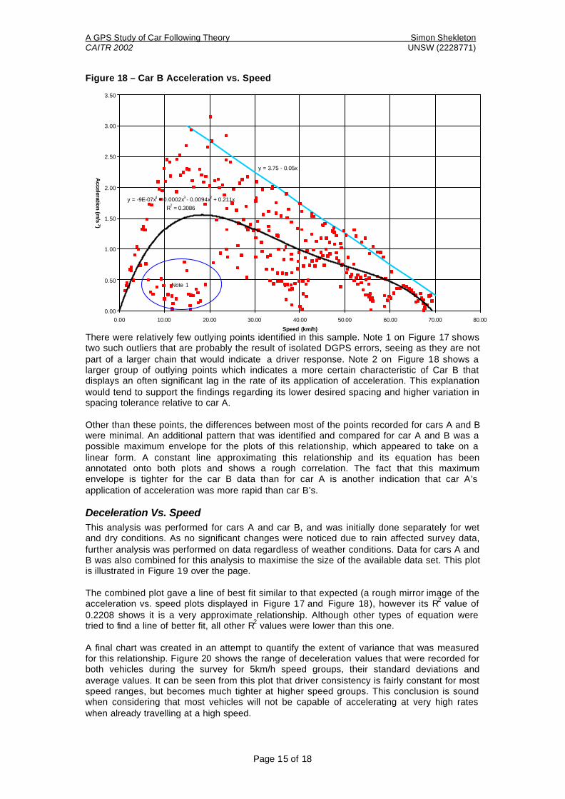
Figure 18 – Car B Acceleration vs. Speed

y = -9E-07x4 + 0.0002x3 - 0.0094x2 + 0.211x

R2 = 0.3086

0.00

0.50

1.00

1.50

2.00

2.50

3.00

3.50

0.00 10.00 20.00 30.00 40.00 50.00 60.00 70.00 80.00

Speed (km/h)

Acceleration (m

/s2)

y = 3.75 - 0.05x

Note 1

There were relatively few outlying points identified in this sample. Note 1 on Figure 17 shows two such outliers that are probably the result of isolated DGPS errors, seeing as they are not part of a larger chain that would indicate a driver response. Note 2 on Figure 18 shows a larger group of outlying points which indicates a more certain characteristic of Car B that displays an often significant lag in the rate of its application of acceleration. This explanation would tend to support the findings regarding its lower desired spacing and higher variation in spacing tolerance relative to car A. Other than these points, the differences between most of the points recorded for cars A and B were minimal. An additional pattern that was identified and compared for car A and B was a possible maximum envelope for the plots of this relationship, which appeared to take on a linear form. A constant line approximating this relationship and its equation has been annotated onto both plots and shows a rough correlation. The fact that this maximum envelope is tighter for the car B data than for car A is another indication that car A’s application of acceleration was more rapid than car B’s.

Deceleration Vs. Speed This analysis was performed for cars A and car B, and was initially done separately for wet and dry conditions. As no significant changes were noticed due to rain affected survey data, further analysis was performed on data regardless of weather conditions. Data for cars A and B was also combined for this analysis to maximise the size of the available data set. This plot is illustrated in Figure 19 over the page. The combined plot gave a line of best fit similar to that expected (a rough mirror image of the acceleration vs. speed plots displayed in Figure 17 and Figure 18), however its R2 value of 0.2208 shows it is a very approximate relationship. Although other types of equation were tried to find a line of better fit, all other R2 values were lower than this one. A final chart was created in an attempt to quantify the extent of variance that was measured for this relationship. Figure 20 shows the range of deceleration values that were recorded for both vehicles during the survey for 5km/h speed groups, their standard deviations and average values. It can be seen from this plot that driver consistency is fairly constant for most speed ranges, but becomes much tighter at higher speed groups. This conclusion is sound when considering that most vehicles will not be capable of accelerating at very high rates when already travelling at a high speed.


of 18

Figure 19 – Combined Deceleration vs. Speed

y = 4E-06x4 - 0.0005x3 + 0.0219x2 - 0.3516x

R2 = 0.2208

-3.50

-3.00

-2.50

-2.00

-1.50

-1.00

-0.50

0.000 10 20 30 40 50 60

Speed (km/h)

Deceleration (m

/s2)

Figure 20 – Deceleration vs. Speed Variation

0.69 0.690.54 0.47 0.50

0.670.54 0.56

0.650.56

0.26

0.07

-3.5

-3

-2.5

-2

-1.5

-1

-0.5

0

0.5

1

0 to 5

5 to 10

10 to 15

15 to 20

20 to 25

25 to 30

30 to 35

35 to 40

40 to 45

45 to 50

50 to 55

55 to 60

Speed Group (km/h)

Deceleration (m

/s2)

MIN STDEV AVG MAX

Other Analysis The original thesis that pre-empted this paper also covered an analysis of cruising sections to further identify the extent to which drivers may vary their speed unnecessarily during sections of driving where they are not influenced by other vehicles. However, due to the necessary shortening of this paper – these analyses have been excluded.

Conclusions

Suitability of Differential GPS to This Task One of the most important conclusions of this study has been that Carrier Phase Differential GPS does provide an appropriate methodology for conducting car following studies such as this. This conclusion has been based on a number of considerations including:


of 18

Number of Useful Data Points CollectedCar A Car B TOTAL

1270 3144 44141290 2538 38282560 5682 8242

Time Equivalent of Useful Data Collected (Mins)Car A Car B TOTAL

10.58 26.20 36.7810.75 21.15 31.9021.33 47.35 68.68

144Proportion of valid results 48%

Follow Car

Follow Car

TOTAL

Dry ConditionsWet Conditions

Duration of Survey (excluding calibration)

Dry ConditionsWet ConditionsTOTAL

Time Saving: The data collection survey involved in this study was easy to set up and fast to perform. It also worked first time, eliminating the need for follow up surveys. The main time saving element of this study was however, in the dissemination of data. Electronic outputs from the DGPS survey allowed quick and easy sorting of which data points were valid and which were not. The basic location and time requirements for the analysis of car following were automatically entered into Microsoft Excel, saving further hours on previous methods.

Table 2 – Useful Survey Data

Data Quality: The early concerns that the data might not produce a high enough proportion of accurate results to be viable were also dismissed as a result of this survey. Table 2 to the right provides a summary of the number of points, and effective duration of the survey that was deemed to be centimetre accurate. The consistently smooth data chains that were obvious during the data analysis stages of this study reinforce the claim that the standard of survey results was high. Expenses: One potential drawback of this methodology that was not experienced during this project was the cost of the DGPS Leica Geosystems equipment that was used. Associate Prof. Chris Rizzos estimated each receiver to be valued at around $10,000, which would significantly affect the viability of studies that would require the purchase of such systems.

Car Spacing Relationships In summary, it can be stated that the conclusions drawn from the analysis of car spacing relationships undertaken in this study are that: § A linear minimum spacing – speed relationship does exist § This relationship may be slightly exponential for erratic or irregular drivers § This relationship becomes significantly more conservative in wet conditions § The variance of spacing – speed relationships increases proportionally to speed § The nature of this increasing proportion is seen as being linear § Hysteresis effects identified in other studies may not be as clear-cut or prevalent in urban

flow conditions as previously believed

Vehicular Acceleration Characteristics Again it is important to stress the difficulty of making ecumenical conclusions from this study given only two drivers were involved. It is however suggested as a result of the analysis performed that: § A valid envelope could be created for acceleration of vehicle platoons (but would depend

heavily on heavy vehicle concentrations and traffic levels) § An envelope of the same shape could be adapted for different speed environments § An envelope such as this has been tested against external results in Figure 14. § Weather conditions do not significantly affect acceleration or deceleration performance § An envelope similar to Figure 14 could possibly be established for deceleration

characteristics in various speed environments § There appears to be a preferred constant rate of braking deceleration that was similar for

cars A and B, and speculated to be around 2.167m/s2. § Analysis of cruising sections further reinforced the validity of “background” deceleration

rates proposed by Pline (1992), and the regular action of drivers to accelerate in order to make up for these speed lags

§ A pattern exists indicating a relationship between acceleration and speed characteristics of drivers. The pattern was found to best be represented by 4th degree polynomial curves, appears to be stochastic in nature and may be subject to a viable maximum envelope


of 18

Individual Characteristics A number of findings in this study have consolidated the opinion that several elements of car following in practice depend on individual or stochastic effects. These include: § Tolerances for desired spacing and minimum spacing to lead cars § The impact of weather conditions on desired spacing § Acceleration vs. Speed plots indicate that variance in this characteristic is individual for

low to moderate speed environments § Driver consistency also appears to be affected by the individual as identified in speed

group variance plots such as Figure 6, Figure 7, Figure 8 and Figure 9.

Summary This study has provided a number of observations based on the ample accurate car following data that was recorded during the projects carrier DGPS survey. It has established that the methodology that was pioneered as a part of this project is sound, and can potentially simplify and shorten the duration of future studies of this nature. It has also been shown that this method of data collection provides accurate measurements in typical urban environments, despite the restrictions of satellite tracking. Furthermore, the study did not encounter any of the constraints that car following studies have typically experienced due to high speeds, long-range tracking or weather conditions. It is hoped that the data obtained in this study has provided insight into some of the more difficult to measure areas of car following theory. Despite the restrictions associated with involving only two cars in the survey, a number of similarities were identified in driver behaviour that have led to speculation on possible broader relationships. It is also hoped that the data obtained from this study will assist in the accurate calibration of Dr. Hidas’ proposed car following model.

References

1 Hidas, P “A car following model for urban traffic simulation”, Traffic Engineering and Control, Vol 39 No 5, May 1998, p300-305

2 Traffic Engineering Handbook, 4th Ed. (ed. JL Pline), Institution of Transportation Engineers, Prentice Hall, NJ, 1992, p37-41

3 Introduction to GPS (Global Positioning System), Leica Geosystems, Switzerland, 2000, Volumes 1-5

4 http://www.colorado.edu/geography/gcraft/notes/gps/gps.html#DifTechs

5 http://www.trimble.com/gps/what.html.

6 Gipps, P.G. A behavioural car-following model for computer simulations, Transpn Res. B, 15B, 1981, p105-111

7 Benekohal, RF and Treiterer, J, CARSIM: Car-following model for simulation of traffic in normal stop-and-go conditions, Transpn Res. Rec. 1194, Transportation Research Board, Washington, DC, 1988, p99-111

8 Parker, MT, The effect of heavy goods vehicles and following behaviour on capacity at motorway roadwork sites. Traff. Engng Control, 37(9), September 1996, 524-531

9 Chen, S, Sheridan, TB, Kusonoki, H, Komoda, N. Car-following measurements simulations, and a proposed procedure for evaluating safety, Analysis, Design and Evaluation of Man-Machine Systems 1995: Vol 2, Pergamon, Oxford, 1995, p529-34.

10 Ozaki, H, Reaction and anticipation in the car-following behaviour. In: Transportation and Traffic Theory (Ed. CF Daganzo), Elsevier Science Publishers, 1993.

a gps study of car following theory - traffic engineering

Documents