Powder Technology 338 (2018) 548–562

Contents lists available at ScienceDirect

Powder Technology

j ourna l homepage: www.e lsev ie r .com/ locate /powtec

A GPU-based coupled SPH-DEM method for particle-fluid flow withfree surfaces

Yi He a,⁎, Andrew E. Bayly a, Ali Hassanpour a, Frans Muller a, Ke Wu b, Dongmin Yang b

a School of Chemical and Process Engineering, University of Leeds, Leeds LS2 9JT, UKb School of Civil Engineering, University of Leeds, Leeds LS2 9JT, UK

⁎ Corresponding author.E-mail address: y.he1@leeds.ac.uk (Y. He).

https://doi.org/10.1016/j.powtec.2018.07.0430032-5910/© 2018 The Authors. Published by Elsevier B.V

a b s t r a c t

a r t i c l e i n f o

Article history:Received 11 April 2018Received in revised form 8 July 2018Accepted 14 July 2018Available online 17 July 2018

Particle-fluid flows with free-surfaces are commonly encountered inmany industrial processes, such as wet ballmilling, slurry transport andmixing. Accurate prediction of particle behaviors in these systems is critical to estab-lish fundamental understandings of the processes, however the presence of the free-surface makes modellingthema challenge formost traditional, continuum,multi-phasemethodologies. Coupling of smoothed particle hy-drodynamics and discrete element method (SPH-DEM) has the potential to be an effective numerical method toachieve this goal. However, practical application of this method remains challenging due to high computationaldemands. In thiswork, a general purposed SPH-DEMmodel that runs entirely on aGraphic ProcessingUnit (GPU)is developed to accelerate the simulation. Fluid-solid coupling is based on local averaging techniques and, toaccelerate neighbor searching, a dual-grid searching approach is adapted to a GPU architecture to tackle thesize difference in the searching area between SPH and DEM. Simulation results compare well with experimentalresults on dam-breaking of a free-surface flow and particle-fluid flow both qualitatively and quantitatively,confirming the validity of the developedmodel. More than 10million fluid particles can be simulated on a singleGPU using double-precision floating point operations. A linear scalability of calculation time with the number ofparticles is obtained for both single-phase and two-phase flows. Practical application of the developed model isdemonstrated by simulations of an agitated tubular reactor and a rotating drum, showing its capability in han-dling complex engineering problems involving both free-surfaces and particle-fluid interactions.

© 2018 The Authors. Published by Elsevier B.V. This is an open access article under the CC BY-NC-ND license(http://creativecommons.org/licenses/by-nc-nd/4.0/).

Keywords:GPUSmoothed particle hydrodynamicsDiscrete element methodFluid-particle interactionFree surface flowSolid-liquid flow

1. Introduction

Understanding particle behaviors in free-surface flows is crucial tomany natural phenomena and industrial processes, such as debrisflow [1], wet ball milling [2, 3], slurry transport [4], mixing and separa-tion in chemical andmineral processing [5–7] and additivemanufactur-ing [8]. Despite wide popularity, application of traditional grid-basedmethods, such as coupled computational fluid dynamic (CFD) and dis-crete element method (DEM), to handle particles in free-surface flowsis still challenging due to the presence of free-surfaces, especiallysplashing and fragmentations [9–11]. Additional detection algorithmsare required to track the free surfaces for grid-based Eulerian methods,such as volume of fluid [9], marker-and-cell [10] and level-set method[11]. In addition, numerical diffusion may arise due to advectionterms. On the other hand, grid-based Lagrangian methods face prob-lems of mesh distortion, which requires expensive mesh re-generation.The presence of splashing and fragmentations requires a numericalmethod which can handle the discrete nature of the free-surfaceflows. SPH, as ameshlessmethod, shows strong potentials in this regard

. This is an open access article under

as it discretize the fluid into a set of particles, thus allowing the dynam-ics of the free-surface flows to be readily captured. Since the pioneerwork of Gingold and Monaghan [12], SPH has been widely used tomodel free-surface flows in many fields [13]. It has been recentlyextended to deal with solid particles in free-surface flows by couplingSPH with DEM [7, 14–17]. Nevertheless, application of this method toengineering problems remains limited due to associated high computa-tional cost. This is especially the casewhen complexmoving boundariesare present. Thus, a high performance implementation of the SPH-DEMmethod is necessary for applications in engineering practice.

Coupling of SPH and DEM enables a unified Lagrangian particle-based method, well suited for applications where free-surfaces andstrong fluid-particle interactions coexist. Approaches for coupling themomentum transfer between the fluid and particles can be classifiedinto two groups: resolved and unresolved methods. In the resolvedmethod the SPH particles are significantly smaller than the solid parti-cles and the flow around the solid particles is explicitly resolved. Inthe unresolved method the SPH particles are of a comparable size ofthe solid particles and empirical force correlations are used to capturethe momentum transport between phases. For resolved simulation, avariety of methods have been developed to enable no-slip conditionsat solid surfaces. Potapov et al. [18] coupled SPH with DEM to simulate

the CC BY-NC-ND license (http://creativecommons.org/licenses/by-nc-nd/4.0/).

549Y. He et al. / Powder Technology 338 (2018) 548–562

shear flow of neutrally buoyant particles, where no-slip boundarycondition is enabled by placing SPH particles inside large solid particles[19]. Densities of the interior SPH particles are updated in the samemanner as the fluid SPH particles while moving the interior SPH parti-cles with the solid particles. This approach was verified with experi-mental results on the drag force and size of the wake for fluid flowaround a circular cylinder. Canelas et al. [20] coupled SPH with aso-called distributed contact DEM, where the solid body is representedby a set of small particles with fixed relative position. The interactionbetween fluid and solid particles are calculated in a manner similar tothemethodology of dynamic boundary conditions [21]. The interactionsamong solid bodies are calculated through the small constituent parti-cles by means of soft-sphere collision model. This model shows goodcomparison with experiments on tracking blocks subjected to a dam-break wave [20] and on a debris flow [22]. Ren et al. [23] also reporteda similar method to study stability of 2D blocks on a slope due towave-structure interaction. Since the fluid resolution has to besufficiently small to resolve flow structure around the particle, highcomputational demand is thus inevitable when dealing with a largenumber of solid particles. The requirement of a larger size of solid parti-cles than the fluid particles further limits their range of applicability,especially considering a wide size distribution of solid particles is com-monly encountered in practical systems.

On the other hand, phase interaction in the unresolved simulation ishandled by empirical force correlations. Both one-way and two-waycoupled SPH-DEM methods have been reported. For example,Komoroczi et al. [24] combined SPH with DEM by treating either DEMparticles as SPH particles or treating SPH particles as DEM particles.Cleary et al. [4, 5] treated the solid bed as a dynamic porousmedia by av-eraging the velocities and porosities of the DEM particles, throughwhich the SPH fluid is able to flow. This one-way coupled method hasbeen applied to predict slurry transport in SAG mills [4] and to modelslurry flow on a double deck vibrating banana screen [5] in mineralprocessing. Sun et al. [6] reported a two-way coupled SPH-DEMmethodin which a boundary model based on variational approach is explicitlyincluded in the momentum equation. A unified boundary representa-tion is enabled for both phases, eliminating the redundantwall particlesfor the fluid phase. Similarly, Robinson et al. [17] developed a coupledSPH-DEM method based on the locally averaged Navier-Stokes equa-tions. The model showed good agreement with sedimentation testcases with increasing complexity, namely, settling of single sphere,constant block of particles and multiple particles. The fully coupledSPH-DEMmethod is gainingpopularity in different engineering applica-tions, including fluid-particle-structure interaction problem withfree-surface flow [14, 15] and landslide generated surge waves [16]and particle separation due to density difference in waste recycling[7]. To date, however, most of these studies are concernedwith 2D sim-ulation [14–16] or limited to a very small scale [7, 17], therefore, devel-oping a general SPH-DEMmodel capable of accelerating simulation is ofgreat importance for practical problems in engineering applications.

Computational efficiency of numerical methods is closely related tothe progress of hardware architecture. GPU-based parallelism hasbeen increasingly applied to speedup simulations of particle-based nu-merical methods due to high memory bandwidth and instructionthroughput offered by GPU processors, such as Molecular Dynamics[25, 26], Lattice Boltzmann Method [27–29], SPH [30, 31] and DEM[32–36]. GPU-based implementations show orders of magnitude fasterthan their serial counterparts, making it very attractive for schemesthat can make use of the single instruction multiple data architecture.Due to the locality of particle interactions, both SPH and DEM schemesrequire identification of neighboring particles. In pure SPH models theinteraction length is greater than twice the particle diameter, where inpure DEM simulations there is no longdistance force and the interactionsearch area is approximately the solid particle diameter. In coupledSPH-DEM systems, the interactions between different particle typesleads to increased complexity. To accelerate neighbor searching on

GPU, different algorithms have been reported, including the k-d treemethod [37] and spatial subdivision approaches, such as the boundingvolume hierarchy method [38, 39] and the uniform grid method [35].The k-d tree structure needs to be reconstructed at every time step,thus not suitable for discrete methods while the spatial subdivisionapproaches are limited by the fact that the grid size needs to be largeenough to host the largest particles. Application of these searchingmethods mentioned above to SPH-DEM is thus not straightforward,especially on a GPU platform. A general purpose SPH-DEM programalso needs to be efficient at GPU memory management. To the best ofour knowledge, coupling of SPH and DEM methods that run entirelyon a GPU platform has yet to be reported.

Starting from the theoretical background, this work will address thedevelopment of a general purposed GPU-based SPH-DEM method indetail. A dual-grid searching approach is incorporated to handle the dif-ference in the particle interacting range between SPH and DEM. Modelvalidation and performance analysis of the GPU-based model will beevaluated for both the single phase and the particle-fluid flows, respec-tively. Practical application of the GPU-based model to chemicalengineering will be illustrated by the simulating free-surface flows inan agitated tubular reactor and particle-fluid flows in a rotating drum.The paper is organized as follows: the model formulation is firstpresented in Section 2 followed by a detailed description of the GPUimplementation, including the neighbor searching method, memorymanagement and program flow. Then, the validation, engineeringapplication and performance of the developed model in handling bothsingle-phase flow and particle-fluid flow with free-surfaces areaddressed separately in Section 3.

2. Model description and GPU implementation

To achieve unresolved simulation, different approaches to coupleDEM to SPH have been reported [6, 14–17], which are essentiallysolving governing equations of the conventional Two Fluid Model(TFM) [40] in the framework of SPH, which are given as,

∂ ερ fð Þ∂t

þ ∇∙ ερ fuð Þ ¼ 0 ð1Þ

∂ ερ fuð Þ∂t

þ ∇∙ ερ fuuð Þ ¼ −∇P−Sp þ ∇∙ ετ fð Þ þ ερ fg ð2Þ

with ρf the fluid density, P pressure acting on the fluid phases, τf theviscous stress tensor and g the acceleration due to gravity. ε is the vol-ume fraction of fluid in each cell. Sp is the source term due to the rateof momentum exchange between the fluid phase and the solid phase.The coupling strategy adopted here is similar to that proposed byRobinson et al. [17]. In this section, an overview of the SPH and theDEM methods used to discretize the governing equations and thestrategy of phase coupling are provided. A detailed description of theforce models used in DEM can be found elsewhere [41–43]. For ease ofreading, the fluid particles are labeled as particle a and b while thesolid particles are labeled as particle i and j.

2.1. Fluid phase: SPH

The methodology behind SPH is based on the theory of integralinterpolants, the interpolated value of a function A(r) at position r isexpressed as,

A rð Þ ¼Z

A r0ð ÞW r−r0j j;hð Þdr0 ð3Þ

where the kernel function W(|r− r′|,h) tends to delta function whenthe interpolation domain is infinitely small. The size of the interpolationdomain is characterized by a smoothing length h. In SPH, fluid isdiscretized into individual particles with each carrying a set of

DEM boundary

Fluid particle

Compact support

SPH boundary particle

Fig. 1. Boundary treatment used in SPH calculation: boundary particles acting as bothdummy fluid particles and repulsive particles.

550 Y. He et al. / Powder Technology 338 (2018) 548–562

associated properties, such as density, pressure and momentum. Thefluid particles follow the flow due to pressure gradient, viscous shearand body force while acting as interpolation points for their neighbors.The integral interpolant at the position of the particle is approximatedby,

A rað Þ ¼Xb

Abmb

ρbW rabj j;hð Þ ð4Þ

withmb and ρb themass and density of particle b, |rab| being thedistancebetween two fluid particles. The summation is taken over all particleswithin the support domain of particle a.

The kernel function W(|rab|,h)must obey a number of mathematicconstraints, including positivity, monotonically decreasing, compactsupport and normalization. In this study, theWendland kernel functionis used since it can achieve a good balance between numerical accuracyand computational cost [44].

W rabj j;hð Þ ¼ αD 1−q2

� �41þ 2qð Þ 0≤q≤2 ð5Þ

where αD is 7/8πh3 in 3D. q = |rab|/h. In practice, the kernel functionvanishes when the particle separation is greater than 2h to achieve acompact support domain.

2.1.1. Continuity equationApplying the SPH particle approximation, the continuity equation of

Eq. (1) can be written as,

dρa

dt¼Xb

mbvab∇aWab rabj j;hð Þ ð6Þ

with ∇aW(|rab|,h) the gradient of the kernel function at the position ofparticle a, and vab = va − vb is the velocity vector. ρ denotes the super-ficial fluid density defined as ρa ¼ ερ f , with ε the volume fraction offluid and ρf the intrinsic fluid density.

2.1.2. Equation of stateIn the weakly compressible SPH schemes [45], fluid particles are

driven by local pressure gradient. Pressure is expressed as a functionof the fluid density, giving a quasi-incompressible equation of state asfollows:

P ¼ Bρa

ερ0

� �γ

−1� �

ð7Þ

with γ=7 and ρ0 reference density of the fluid. B is a pressure constantdetermines the speed of sound by cs2 = γB/ρ0. The density fluctuation influid flow is proportional to M2 where M is the Mach number. Bylimiting the Mach number, the flow can be considered practically in-compressible. To limit the density variation within 1%, the coefficientB can be calculated as,

B ¼ 100ρ0

γv2max ð8Þ

2.1.3. Momentum equationThe momentum equation of Eq. (2) in SPH form is given by,

dvadt

¼ −Xb

mbPa

ρ2a

þ Pb

ρ2b

þ Rab

" #∇aWab rabj j;hð Þ þΠab þ Sa þ g ð9Þ

with P the pressure due tofluid phase,Πab the viscosity term and Rab theterm due to tensile instability and Sa the couple term due to solid parti-cles. The symmetrical form of the pressure gradient term is taken inorder to reduce error arising from particle inconsistence. The stress

termsΠab representing the viscous diffusion derived by [19] is incorpo-rated into the momentum equation,

Πab ¼Xb

mb μa þ μbð Þrab∙∇aWab rabj j; hð Þρaρb r2ab þ 0:01h2

� � vab ð10Þ

where μ is the dynamic viscosity. In the weakly compressible SPH,tensile instability is often attributed as the cause of unphysical particleclumping. This phenomenon is especially significant in materials withan equation of state which can give rise to negative pressures, whichreduces numerical accuracy due to the uneven particle distribution. Toremove the instability, [46] introduced an additional pressure betweenparticles to prevent particle from forming small clumps. This artificialpressure term Rab is added to the momentum equation, given as,

Rab ¼ 0:01Pa

ρ2a

þ Pb

ρ2b

!W rabj j;hð ÞW Δp;hð Þ

� �4

ð11Þ

where Δp is the initial particle spacing.

2.1.4. Moving the particlesTo keep an orderly flow of particle, the particles aremoved using the

XSPH variant,

dradt

¼ va−ϵXb

mb

ρabvabWab rabj j;hð Þ ð12Þ

where ρab ¼ ðρa þ ρbÞ=2 and ϵ is a problem-dependent constant,ranging from 0 to 1. It moves a particle at a velocity close to the averagevelocity of its neighbors. In this study, ϵ is set to 0.3.

2.1.5. Boundary treatmentWhen a SPH particle approaches a rigid boundary, the support

domain of its kernel will be truncated by the boundary. Ideally, theboundary treatment should compensate for the lack of particles beyondthe boundary and provide enough repulsive force to prevent particlesfrom penetration. Different treatments have been proposed to thisend, including kernel re-normalization [47], ghost particles [48], layersof fixed fluid particles, repulsive particles [45] and dynamic particles[49–51]. Sun et al. [6] introduced a correction to the SPH approximationwhere the boundary information are explicit included without usingextra wall particles. Together with level-set functions, a unified bound-arywas enabled for both the solid phase and thefluid phase. In the pres-ent study, a generalized wall boundary treatment that is capable ofhandling arbitrarily shaped geometries was adopted [52]. As shown inFig. 1, solid wall is discretised into dummy particles whose propertiesdo not evolve with time. These wall particles provide support for thekernel interpolants of the fluid particles. The pressure and velocity atthe position of a wall particle is interpolated from surrounding fluid

551Y. He et al. / Powder Technology 338 (2018) 548–562

particles to ensure a non-slip boundary condition of the solid walls,which are given by,

vw ¼ 2va−

Xb

vbWab rabj j; hð ÞXb

Wab rabj j;hð Þ ð13Þ

Pw ¼

Xf

P fWwf rwfj j; hð Þ þ g−awð ÞXf

ρ frwfWwf rwfj j; hð ÞXf

Wwf rwfj j; hð Þ ð14Þ

ρw ¼ ρ0Pw

Bþ 1

� �1γ

ð15Þ

with va the prescribedwall velocity, aw the acceleration of thewall and |rwf| being the distance between fluid particle and wall particle. In prac-tice, however, wall penetration cannot be fully avoid where violentfluid-wall interactions exist. Therefore, in this study, the repulsiveforce proposed byMonaghan [45] is combinedwith the above boundarytreatment to fully prevent wall penetration.

2.2. Solid phase: DEM

In DEM, the motion of solid particles is tracked by Newton’s secondlaw of motion, written as,

mdvdt

¼ F f þ Fc þmg ð16Þ

Idωdt

¼ T f þ Tc ð17Þ

where m, I, v and ω are, the mass, inertia, translational and rotationalvelocities of the element, respectively. The force and torques acting oneach particle consists of several contributions, including the hydrody-namic components, Ff and Tf, arising from fluid-particle interaction,the collision components, Fc and Tc, due to solid-solid interaction andmg the gravity. The collisions between particles are handled by asoft-sphere model that allows for inter-particle overlap. The collisionforce includes the normal contact force Fn, normal damping force Fd,n,tangential contact force Ft and tangential damping force Fd, t. Thenormal contact is described by Hertz theory while tangential elasticfrictional contact is based on Mindlin and Deresiewicz theory [53]. Thenormal and tangential contact forces are given as,

Fn ¼ 43E�R�1=2δ3=2n n̂ ð18Þ

Ft ¼ −δtμt Fnj jδtj j 1− 1−

min δtj j; δt; max� �δt; max

� �3=2" #ð19Þ

in which the R∗, E∗and δt, max are calculated as,

1R� ¼

1Ri

þ 1R j

ð20Þ

1E�

¼ 1−ν2i

Eiþ1−ν2

j

E jð21Þ

δt; max ¼ 2−νð Þ2−2ν

μtδn ð22Þ

with Ri and Rj being the radius of two particles in contact. E and ν are theYoung’s Modulus and Poisson’s ratio of solid particles, respectively. δnand δt represent the overlap in normal and tangential directions and μtis the sliding friction.

The equations used to calculate damping in normal and tangentialdirections are given by,

Fd;n ¼ −cn 8m�E�ffiffiffiffiffiffiffiffiffiffiR�δn

p� �1=2vn ð20Þ

Fd;t ¼ −ct 6μtmE� Fnj jffiffiffiffiffiffiffiffiffiffiffiffiffiffiffiffiffiffiffiffiffiffiffiffiffiffiffiffiffi1− δtj j=δt; max

pδt; max

!1=2

� vt ð21Þ

where cn and ct are the normal and tangential damping coefficient,respectively. The normal damping coefficient can be directly linked tothe restitution coefficient e in the normal direction by,

cn ¼ − lne=ffiffiffiffiffiffiffiffiffiffiffiffiffiffiffiffiffiffiffiffiffiffiffiπ2 þ ln2e

qð23Þ

Thenormal restitution coefficient e is defined as the ratio of post-col-lisional contact velocity to pre-collisional contact velocity.

The collision torque Tc is composed of the torque due to the tangen-tial force Tt and the torque Tr due to particle rolling friction resultingfrom the elastic hysteresis losses or viscous dissipation [54], calculatedas,

Tt ¼ Ft þ Fd;t� �� R ð24Þ

Tr ¼ μrR Fnj jω̂n ð25Þ

where μr is the rolling friction and ω̂n ¼ ωn=jωnj with ωn the angularvelocity.

2.3. Phase coupling

The local porosity at the position of fluid particle a is calculated by asummation over neighboring DEMparticles within a coupling length hc,given as,

εa ¼ 1−Xj

Waj hcð ÞV j ð26Þ

with Vj the volume of DEM particle j,Waj( hc) the SPH kernel and hc thecoupling length for the interaction between two phases. The couplinglength should be larger than the diameter of solid particle but smallenough to capture local feature of the porosity field. Here, the couplinglength is set to be same as the SPH smoothing length.

For the solid particles, forces due tofluidflowaremodelled. The totalfluid force can be split into a pressure gradient force and a drag force.

Fi ¼ −V i −∇P þ ∇∙τð Þ þ Fd ð27Þ

with Vi the particle volume, ∇P the pressure gradient and Fd the dragforce. The pressure gradient is evaluated at solid particle i using aShepard corrected SPH interpolation [55], given as,

−∇P þ ∇∙τð Þi ¼1X

b

mb

ρbWab hbð Þ

Xb

mb

ρbθbW ib hbð Þ ð28Þ

θa ¼ −Xb

mbPa

ρ2a

þ Pb

ρ2b

!∇aWab hbð Þ þΠab ð29Þ

Thefluid-particle drag force Fd depends on the local porosity and rel-ative velocity between fluid and particle. For the dense particle fluidflow, the drag model of Ergun and Wen & Yu [56, 57] is used, which isbased on experimental measurements.

Fd ¼ βV i

1−εu−vð Þ ð30Þ

552 Y. He et al. / Powder Technology 338 (2018) 548–562

with β the interphase momentum exchange coefficient, which is givenby,

β ¼150

μ 1−εð Þ2εd2i

þ 1::751−εð Þρ f

diu−vij j ε < 0:8ð Þ

34CD

ε 1−εð Þdi

ρ f u−vij jε−2:65 ε > 0:8ð Þ

8>>><>>>:

ð31Þ

where CD is the drag coefficient. It can be calculated as,

CD ¼24 1:0þ 0:15Re0:687p

� �Rep

Rep ≤1000� �

0:44 Rep > 1000� �

8><>: ð32Þ

in which the particle Reynolds number Rep is defined as Rep = ρdpε|u− vp|/μ.

The rate ofmomentumexchange in the right hand of Eq. (2) for eachSPH particle is calculated by a weighted average of fluid-particlecoupling force acting on the surrounding DEM particles within the cou-pling length hc, so that Newton’s third law of motion is satisfied, whichis given by,

Sa ¼ −ma

ρa

Xj

1Xb

mb

ρbWab hbð Þ

FiWaj hcð Þ ð33Þ

(a) (b)

(d)

Level 1Level 2

Level

Fluid particle

Solid particleTargeted solid particle

Identified neighboring solid particles

Targeted fluid particle

Identified neighboring fluid particles

Level

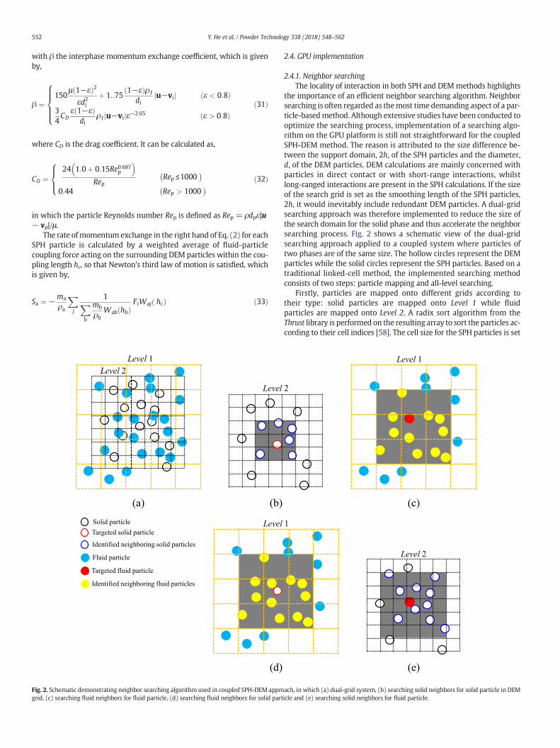
Fig. 2. Schematic demonstrating neighbor searching algorithm used in coupled SPH-DEM approgrid, (c) searching fluid neighbors for fluid particle, (d) searching fluid neighbors for solid part

2.4. GPU implementation

2.4.1. Neighbor searchingThe locality of interaction in both SPH and DEMmethods highlights

the importance of an efficient neighbor searching algorithm. Neighborsearching is often regarded as themost time demanding aspect of a par-ticle-basedmethod. Although extensive studies have been conducted tooptimize the searching process, implementation of a searching algo-rithm on the GPU platform is still not straightforward for the coupledSPH-DEM method. The reason is attributed to the size difference be-tween the support domain, 2h, of the SPH particles and the diameter,d, of the DEM particles. DEM calculations are mainly concerned withparticles in direct contact or with short-range interactions, whilstlong-ranged interactions are present in the SPH calculations. If the sizeof the search grid is set as the smoothing length of the SPH particles,2h, it would inevitably include redundant DEM particles. A dual-gridsearching approach was therefore implemented to reduce the size ofthe search domain for the solid phase and thus accelerate the neighborsearching process. Fig. 2 shows a schematic view of the dual-gridsearching approach applied to a coupled system where particles oftwo phases are of the same size. The hollow circles represent the DEMparticles while the solid circles represent the SPH particles. Based on atraditional linked-cell method, the implemented searching methodconsists of two steps: particle mapping and all-level searching.

Firstly, particles are mapped onto different grids according totheir type: solid particles are mapped onto Level 1 while fluidparticles are mapped onto Level 2. A radix sort algorithm from theThrust library is performed on the resulting array to sort the particles ac-cording to their cell indices [58]. The cell size for the SPH particles is set

(c)

(e)

2

Level 1

1

Level 2

ach, in which (a) dual-grid system, (b) searching solid neighbors for solid particle in DEMicle and (e) searching solid neighbors for fluid particle.

Data Initialization

Update DEM particles: velocities & positions

Map SPH particles to searching grid

Calculate:density change rate, internal forces,viscous forces and external forces

Calculate fluid force on DEM particles

Calculate reaction force on SPH particles

Update SPH particles:velocities and positions

Calculate properties of SPH fluid particles:porosity, superficial density and pressure

DEM

Particle generation

Build neighbor list

Update contact history

Calculate particle-particle and particle-wall interactions

Synchronized with SPH time?

Calculate properties of SPH wall particles: porosity, pressure and velocities.

End of calculation? Transfer data from GPU to CPU

Reach output time?

Output results to filesEnd

Transfer data from CPU to GPU

Criteria for rebuilding DEM neighbor list?

Criteria for remapping SPH particles?

SPH

Yes

No

Yes

No

Yes

NoNo

Yes

Yes

No

Fig. 3. Flow chart of the algorithm of the coupled SPH-DEM method. The steps in theshaded boxes are conducted on the GPU.

553Y. He et al. / Powder Technology 338 (2018) 548–562

as 2h + ΔSPH while it is set as dmax + ΔDEM for the DEM particles, inwhich dmax is the maximum particle diameter. Consequently, only par-ticles in the neighboring cells contribute to the update of a same phase(Fig. 2(b) and 2(c)). The searching area is shaded for illustrationpurposes in Fig. 2. The purpose of introducing an extra searching gapΔ is to avoid conducting the particle mapping and searching at everytime step. A large value of Δ means more time are needed to conductneighbor searching for each time. It is thus a balance between the fre-quency of searching and the time cost of each searching routine. Itsvalue depends on factors like the particle velocities and solid concentra-tion, but normally smaller than the particle size. In this study, it is set as0.3 times of the particle size. Potential neighbors are then identified bylooping through all levels of the searching grid. For SPH particles, thefluid neighbors are detected from Level 2 while its solid neighbors aresearched on Level 1. For the DEM particles, the contact detectionbetween solid particles is conducted on Level 1 while the interactionwith fluid particles is performed on Level 2. For interactions betweenphases, the search area depends on the size ratio between the size ofthe SPH particle support domain and the DEM particle size. To findneighboring DEM particles, the SPH particle is mapped into Level 1, asshown in Fig. 2(e). In this illustrative example, ⌈2h/d⌉= 3 (where thenomenclature ⌈x⌉ returns the smallest integer larger than x). Searchingis therefore conducted by looping through the three surrounding layersof the DEM cells. On the other hand, to find neighboring SPH particlesfor a given DEM particle, searching is only performed within the sur-rounding SPH cells and the mapped cell itself as ⌈d/2h⌉= 1, as shownin Fig. 3(d).

2.4.2. Memory managementA unique feature of the DEM calculation is the need to record the

contact status between two contacted particles. It is used to determinethe friction status, either in static friction or in dynamic friction. If plasticdeformation or inter-particle bonding is considered, a large amount ofmemory is required to keep the contact history information [43].Additionally, double-precision floating point accuracy is required tominimize numerical errors. Consequently to enable the efficient solu-tion of large-scale problems, it is important to optimize the algorithmto balance memory consumption and computing efficiency. To thisend, a neighbor list is only constructed for the DEM particles as eachSPH particle can host a large amount of neighbors due to its large sizeof support domain. Instead, the step of particlemapping for the SPHpar-ticles is conducted occasionally while the step of all-level searching isconducted at every time step. The reconstruction of DEM neighbor listand the particle mapping step for SPH particles are triggered when ac-cumulated displacement of any particles exceeds a specified threshold:ΔDEM/2 for DEM particles and ΔSPH/2 for SPH particles, respectively.

In this study, both the neighbor list and associated contact history in-formation are saved in the global memory on the GPU. Each time step,neighbor searching and force calculations require frequent access tothis data. The memory layout has therefore been optimized to boostthe efficiency of data fetching. GPU threads are grouped into warps of32 threads and each memory operation is issued per warp, meaningthat one memory fetch can return a cache line of 128 bytes. Conse-quently to promote coalesced memory access, and therefore maximizethe efficiency of each fetch, the neighbor index and contact historydata arrays of each DEM particle are organized in a column-majorpattern.

2.4.3. Program flowThe coupled SPH-DEM method was implemented using C++ and

Compute Unified Device Architecture (CUDA) developed by NVIDIA.The GPU program was formulated using a single-program multiple-data (SPMD) technique, where the same program is executed by multi-ple threads simultaneously. Due to the discrete nature of the particlemethods, GPU threads are assigned to each particle (either DEM orSPH particle). As a result, neighbor searching, force calculation and

time integration of the equation of motion can be carried outindependently for each particle using different GPU kernel functions.For efficient use of the GPU memory, parameters that remain thesame during simulation, such as material properties, are stored in theconstant memory (a type of read-only memory on the GPU with fastdata fetching) while other particle-related information, including posi-tions, velocities, forces and contact histories, are stored in the globalmemory on the GPU.

Fig. 3 shows the flow chart of the algorithm that runs on a singleGPU. The whole program can be divided into two major parts: DEMcalculation and SPH calculation. For each type of calculation, there arethree major components: i) neighbor searching (DEM) or particlemapping (SPH), ii) force computation and iii) time integration of the

Fig. 4.Particle representation of thedam-break test case.Wdenotes thewidthof thewatercolumn. Blue particles represent the solid wall while red particles represents the fluid.(The side wall and moving gate wall are not shown for clarity.)

554 Y. He et al. / Powder Technology 338 (2018) 548–562

equation of motion using an explicit time integration method (forwardEuler method). The time step for time integration in SPH is limited bythe CFL-condition based on the artificial sound speed and themaximumflow speed and viscous condition [13] while the time step used forDEM calculation is determined based on a Rayleigh wave propagationcriteria [59].

The program starts by reading pre-defined initial positions and theassociated properties of the SPH particles from files generated from apre-processing step. The solid particles are subsequently randomlygenerated and allowed to settlewithin the required region or the geom-etry. Once this initialization is complete the DEM and SPH calculationsare started. During each step, the DEM calculation are first performedfollowing an order of searching neighbors, updating contact histories,calculating forces and updating the particle velocities and positions.The DEM calculation iterates multiple times until the DEM time is syn-chronized with the SPH time. The SPH calculation is then started bymapping the fluid particles onto the searching grid, namely assigningthefluid particles into axially-aligned cells, ready for neighbor searchingin the following steps. The porosity at the position of each fluid particleis calculated from surrounding solid particles (Eq. (26)). The pressure offluid particles is updated using the equation of state based on the fluidsuperficial density (Eq. (7)). Then, the interaction between fluid parti-cles is calculated by solving the continuity (Eq. (6)) and momentumequations (Eq. (9)). The phase coupling is achieved by calculating thefluid force acting on the solid particles (Eq. (27)) and then the reactionforce on the fluid particles is calculated using a weighted-average of theforces from the solid particles (Eq. (33)). Finally, the fluid particles’density, velocity and position are updated. These calculations are re-peated over the simulation time. It should be noted that the bandwidthbetween CPU and GPU limits the efficiency of memory transfer.Therefore, we only retrieve simulation data occasionally back to theCPU for data recording. With the exception of the data transfer all thecalculations are performed on the GPU by means of issuing a set ofCUDA kernel functions.

3. Results and discussion

In this section, validation, application and performance evaluation ofthe GPU-based models are carried out. The model validation is focusedon the SPH model and the coupled SPH-DEM model as the GPUexecution of the DEMmodel has been validated and applied in previousstudies of powderflowand compaction [41–43]. Dambreak simulationswith single and two-phase flow are chosen for this purpose due to theirsimplicity andwide acceptance as validation tests for free-surfaceflows.The validated models are then applied to two systems: a novel tubularreactor where the fluid flow is agitated by a perforated tube and aquasi-steady solid-liquid flow in a rotating cylindrical drum. Thesewere selected to examine the capability of the models in handlingcomplex systems encountered in engineering practice.

3.1. Single phase flow

3.1.1. Model validation: single phase dam break

3.1.1.1. Validation and effect of fluid resolution.The single phase dam break system modelled here has been widely

used for SPHmethod validation [6, 7, 14, 16] by comparisonwith the ex-perimental results of Koshizuka et al. [60]. The fluid particles are set upinitially on a Cartesian lattice, as shown in Fig. 4.

The predicted flow patterns were compared with those from theexperiments at a series of time instants, as shown in Fig. 5. Particlesare colored by the velocity magnitude. A wedge-shaped water front isgenerated and moves rapidly towards the right after the suddenremoval of the confinement (Fig. 5(a)). The water front starts to deflectand deform once hitting on the vertical wall, a significant amount ofwater is deflected vertically (Fig. 5(b)) and then falls back due to gravity,

generating a plunging surface wave which travels back towards the leftside of the tank (Fig. 5(c) and (d)). The flow patterns agree well withthose observed experimentally, indicating that the present model is ca-pable of qualitatively capturing the flow behavior in the dam-breaking.

The effect of thefluid particle size on thepredictedflowpatternswasinvestigated by comparing the results form 2, 3 and 4 mm fluidparticles. The overall flow patternswere very similar howevermore de-tailed structure was seen with smaller particles. This is illustrated inFig. 6, which compares the flow patterns seen at 0.8 s. It can be seenthat the size of the void formed under the leading front of the waterwave increases with the smaller particle size.

A quantitative estimate of themodel accuracy is made by comparingpredicted and experimental propagation of the wave front beforehitting the right side vertical wall. To this end, two dimensionlessnumbers are defined: the position of the leading wave front x∗and thecharacteristic time t∗, which are given as,

x� ¼ x=a ð30Þ

t� ¼ tffiffiffiffiffiffiffiffiffiffiffi2g=a

pð31Þ

x is the position of the wave front in the horizontal direction; a is thewidth of the water column before collapsing; t is the physical timeand g is gravitational acceleration. As shown in Fig. 7, the SPH slightlyunderpredict the position of the leading front at the initial stage whilea better agreement can be seen after t∗ > 1.5. The fair agreement ofthe results gives a difference within 5% of the predicted value, demon-strating that the model is able to provide accurate quantitative datafor single phase free-surfaceflows. Fig. 7 also shows the effect of particleresolution on the position of the wave front, with decreasing particlesize, the wave front propagates slightly quicker, indicating that a betteragreement can be reached when using finer particle resolution.

3.1.1.2. Performance evaluation.The performance and scalability of the GPU-based SPHmethodwere

evaluated by increasing the dam width in the simulation above from200mm to 12,800 mm, while other dimensions remain the same. Thisincreased the particle number to 14.142 million in the largest

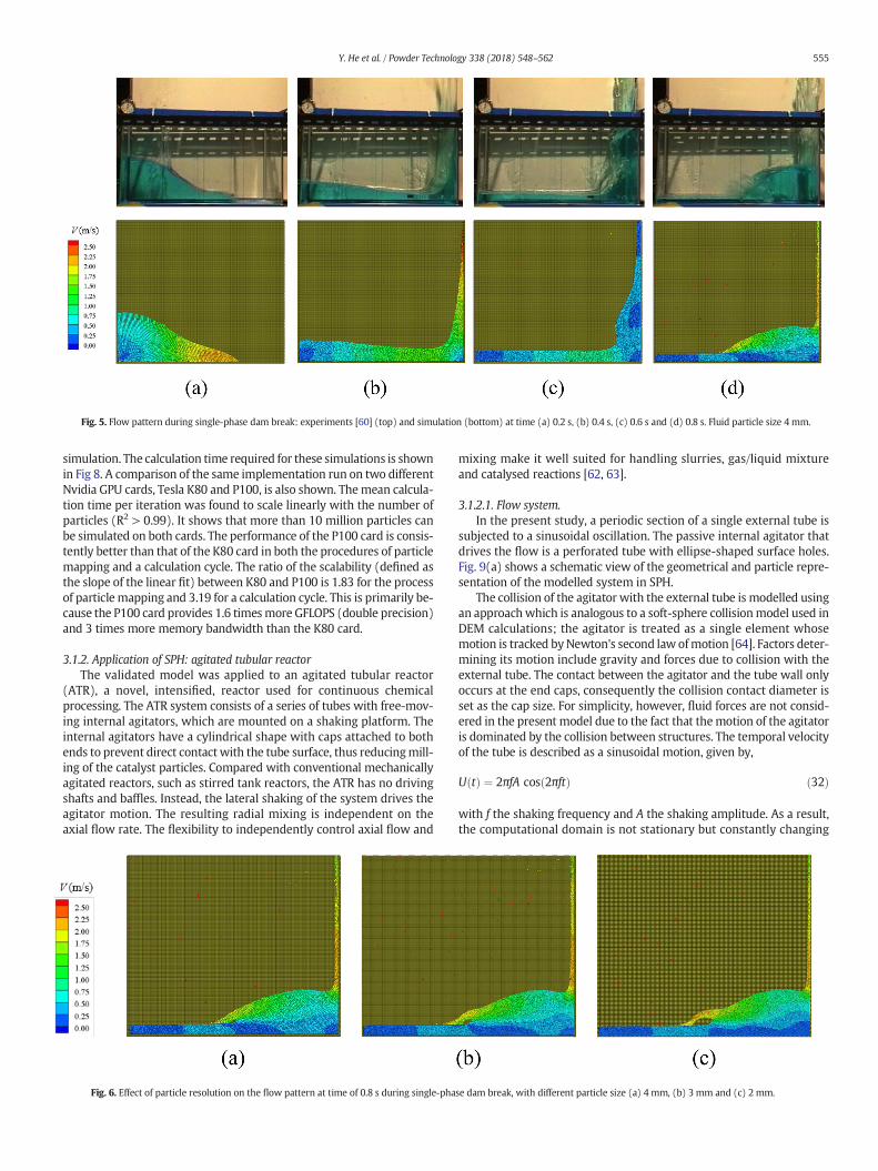
Fig. 5. Flow pattern during single-phase dam break: experiments [60] (top) and simulation (bottom) at time (a) 0.2 s, (b) 0.4 s, (c) 0.6 s and (d) 0.8 s. Fluid particle size 4 mm.

555Y. He et al. / Powder Technology 338 (2018) 548–562

simulation. The calculation time required for these simulations is shownin Fig 8. A comparison of the same implementation run on two differentNvidia GPU cards, Tesla K80 and P100, is also shown. Themean calcula-tion time per iteration was found to scale linearly with the number ofparticles (R2 > 0.99). It shows that more than 10 million particles canbe simulated on both cards. The performance of the P100 card is consis-tently better than that of the K80 card in both the procedures of particlemapping and a calculation cycle. The ratio of the scalability (defined asthe slope of the linear fit) between K80 and P100 is 1.83 for the processof particle mapping and 3.19 for a calculation cycle. This is primarily be-cause the P100 card provides 1.6 timesmore GFLOPS (double precision)and 3 times more memory bandwidth than the K80 card.

3.1.2. Application of SPH: agitated tubular reactorThe validated model was applied to an agitated tubular reactor

(ATR), a novel, intensified, reactor used for continuous chemicalprocessing. The ATR system consists of a series of tubes with free-mov-ing internal agitators, which are mounted on a shaking platform. Theinternal agitators have a cylindrical shape with caps attached to bothends to prevent direct contact with the tube surface, thus reducingmill-ing of the catalyst particles. Compared with conventional mechanicallyagitated reactors, such as stirred tank reactors, the ATR has no drivingshafts and baffles. Instead, the lateral shaking of the system drives theagitator motion. The resulting radial mixing is independent on theaxial flow rate. The flexibility to independently control axial flow and

Fig. 6. Effect of particle resolution on the flow pattern at time of 0.8 s during single-pha

mixing make it well suited for handling slurries, gas/liquid mixtureand catalysed reactions [62, 63].

3.1.2.1. Flow system.In the present study, a periodic section of a single external tube is

subjected to a sinusoidal oscillation. The passive internal agitator thatdrives the flow is a perforated tube with ellipse-shaped surface holes.Fig. 9(a) shows a schematic view of the geometrical and particle repre-sentation of the modelled system in SPH.

The collision of the agitator with the external tube is modelled usingan approachwhich is analogous to a soft-sphere collisionmodel used inDEM calculations; the agitator is treated as a single element whosemotion is tracked byNewton's second law ofmotion [64]. Factors deter-mining its motion include gravity and forces due to collision with theexternal tube. The contact between the agitator and the tube wall onlyoccurs at the end caps, consequently the collision contact diameter isset as the cap size. For simplicity, however, fluid forces are not consid-ered in the present model due to the fact that themotion of the agitatoris dominated by the collision between structures. The temporal velocityof the tube is described as a sinusoidal motion, given by,

U tð Þ ¼ 2πfA cos 2πftð Þ ð32Þ

with f the shaking frequency and A the shaking amplitude. As a result,the computational domain is not stationary but constantly changing

se dam break, with different particle size (a) 4 mm, (b) 3 mm and (c) 2 mm.

Fig. 7. Comparison of the propagation of thewave front as a function of characteristic timebetween SPH results and experiments [61].

Fig. 8. Computational cost of a calculation cycle as a function of the number of particles ondifferent GPU cards. The results are shown in the formof thewall clock time per simulatedtime step averaged over 1000 timesteps.

(a) (b)

Agitator

End cap

Lateral shaking

Fig. 9. (a) Schematic of the cross-section of the reactor tube in the Coflore ATR1 reactor (corepresentation of the simulated ATR system, in which the size of the fluid particle is 0.2mm.

556 Y. He et al. / Powder Technology 338 (2018) 548–562

with the shaking of the external tube, which would complicate themodel implementation and data analysis. In order to enable a stationarydomain, simulations are performed in the reference frame of the shak-ing tube. To this end, an acceleration is imposed to both the agitatorand the fluid, given by,

a tð Þ ¼ −4π2 f 2A sin 2πftð Þ ð33Þ

with a direction opposite to the shaking. Computationally, it is prohibi-tive to model the whole length of the reactor, a section of ATR system isthus modelled with periodic boundary condition applied in the axialdirection. The working fluid is water. Other modelling parameters aresummarized in Table 1, which are typical operational parameters. Atotal physical time of 5s is simulated.

3.1.2.2. Motion of the agitator.The agitator presents a well-behaved periodic motion due to the si-

nusoidal oscillation of the reactor tube. The motion of the agitatorquickly reaches a stable state after the first two periods. The behaviourof the agitator in a typical period are shown in Fig. 10. From phase 0to 0.5π, the reactor tube moves toward the right hand side with a de-creasing velocity, while the agitator accelerates towards the bottom ofthe tube followed by a deceleration when it moves upwards. The

(c)

Fluid

Internal agitatorExternal tube

urtesy AM Technology), (b) Geometrical representation of the agitator and (c) particle

Table 1Parameters used in simulation.

External tubeAmplitude, A (mm) 7.1Frequency, f (Hz) 4.06Diameter, D (mm) 25.4

Internal agitatorInner diameter, Di (mm) 13.8Outer diameter, Do (mm) 14.4Density, ρs (kg/m3) 7800Cap size, Scap (mm) 1.5Moment of Inertia, I (kg·m2) 2.516 × 10-7

Young’s modulus, E (Pa) 1.0 × 108

Poisson ratio, ν 0.3Sliding friction coefficient, μt 0.3Restitution coefficient, e 0.6

Fluid particlesFluid density, ρf(kg/m3) 1000Viscosity, μ (kg/m·s) 0.001

Fig. 10. Evolution of (a) position, (b) translational velocity, (c) velocity magnitude, (d) angular velocity of the agitator in the reference frame of the shaking tube and (e) an illustration ofthe motion of the agitator in the global reference frame, in which phase A=0.581π, B=0.906π, C=1.150π, D=1.393π and E=1.637π.

557Y. He et al. / Powder Technology 338 (2018) 548–562

agitator reaches the highest point around phase A shortly after the tubereverses its moving direction at 0.5π. At this stage, the tube continues tomove to the left hand side at an increasing speed while the agitatorslides down towards the bottom at an increasing speed. The maximumvelocity of the agitator is around 0.076m/s which corresponds to 42% ofthemaximumshaking velocity (0.181 m/s). After the tubepass themid-dle point of its moving region (>1.0π), the agitator reaches the bottomof the tube at phase C. After that, the agitator start to move upward at adecreasing speed.

3.1.2.3. Agitated flow field.Fig. 11(b) shows the contours of fluid velocity magnitude at the five

selected phases marked in Fig. 10(a). Combining the information fromFig. 10(a)-(d), an illustration of the agitator’s motion and the positionof the shaking tube in the global reference frame are given in Fig. 11(a). In general, the motion of the fluid is mainly driven by the shakingof the reactor tube as suggested by the rotation of the fluid as a whole.However, local variations can still be seen due to the presence of the ag-itator. For example, at phase A, local maximum of the fluid particles arefound located at the interstice between the agitator and the reactor,similar to that of the phase E. This is primarily due to the small relativevelocity between the agitator and the reactor tube at these phases. Thefluid particles at the contact region are being squeezed out by the agita-tor. Due to the presence of the surface holes, a repeated pattern of thefluid velocity along the axial direction can be observed at the free sur-face. The complex dynamics captured in the ATR system shows thestrong potential of applying the developed GPU-based SPH in

understanding and further optimizing the design and the operationalconditions of chemical reactors where the free-surface flows present.

3.2. Particle-fluid flow

3.2.1. Model validation: two-phase dam breakTo validate the coupling between SPH and DEM, a two-phase

dam break is simulated and is compared with the experimental re-sults reported by Sun et al. [6]. This test case has also been adoptedto validate coupled SPH-DEM approaches in other studies [7, 15].The water tank has overall dimensions: 200 mm × 150 mm × 150mm, and is split into two volumes by a movable gate 50 mmfrom one end. Water with a depth of 100 mm along with a packedparticle bed are blocked by the gate. The dam break is initiatedby moving the gate upward at a constant speed of 0.68 m/s. Theinitial particle configuration of the SPH-DEM simulation is shownin Fig. 12.

For the solid phase, a total mass of 200 g spherical particles are firstrandomly generated behind the moving gate. Then, they are allowed tosettle under gravity until the total kinetic energy essentially vanishes.For the fluid phase, SPH particles with material properties of water areorderly distributed behind the gate. Other modelling parameter can befound in Table 2.

Fig. 13 compares the simulation with the experiments at a time in-terval of 0.5 s. The SPH particles are colored by volume fraction whilethe DEM particles are colored by the velocity magnitude. The dambreak is initiated by moving the gate upward at a constant velocity of0.68 m/s. With restriction of the vertical gate, particles are driven by

Fig. 11. Velocity profile in a half-filled ATR system at different phases, in which phase A=0.581π, B=0.906π, C= 1.150π, D=1.393π and E=1.637π. Fluid particles are colored byvelocity magnitude in the reference frame of the tube.

558 Y. He et al. / Powder Technology 338 (2018) 548–562

the fluid drag to move along with the flow direction. In comparison,both the fluid and the solid phase observed in experiments are wellreproduced, indicating qualitatively comparable simulation results.The minimum fluid volume fraction produced by the simulation isaround 0.33 which is close to the packing fraction of randomloose packing (0.64). In the simulation, however, the wave front of thewater lags the experiment very slightly, this can be seen in Fig. 13d; inthe experiment the water has reached the left hand wall, where as inthe simulation the water wave has not quite made impact.

Quantitative comparisons of the extent of propagation of the leadingfront of both the fluid and the solid phases are shown in Fig. 14. Thesame dimensionless numbers are used as the previous single phasecase. It can be seen that the simulation matches well with the experi-ments. Discrepancies, however, are seen at initial stage of the dambreak for the fluid phase (0.015 s to 0.035 s) and at the later stage for

Fig. 12. Particle configuration of the two-phase dam break test case for SPH-DEM, solidparticles are not shown. Fluid particles are colored by volume of fraction.

the solid phase (>0.14 s). Several factorsmay contribute to the discrep-ancy, including the use of uncalibrated DEM parameters, such as thefriction coefficient and the restitution coefficient, as also noted byMarkauskas et al. [7], and the lack of the lubrication mechanism in thepresent simulation which would also lead to an underestimation ofthe position of the solid front.

3.2.2. Application of coupled SPH-DEM: rotating drumIn mineral and chemical processing, rotating drums are often used

for mixing or grinding. Water is added to suppress dust or to modifythe operational conditions, leading to a typical slurry flow. In thissection, the GPU-based coupling method is applied to model the parti-cle-fluid flow in a rotating cylindrical drum. The setup is the same asreported in thework of Sun et al. [6]. The predicted results are first com-pared with experiments in terms of the bed shape and dimensions.

Table 2Modelling parameters used in the simulation.

Solid phaseNumber of particles 7762Density (kg/m3) 2500Young's modulus (Pa) 1.0 × 108

Friction coefficient 0.2Rolling friction coefficient 0.01Restitution coefficient 0.9Time step (s) 2.5 × 10-6

Fluid phaseDensity (kg/m3) 1000Viscosity (Pa·s) 8.9×10-4

Fluid resolution (mm) 3.0Boundary particle separation (mm) 2.1Smoothing length, h (mm) 3.9Time step (s) 5×10-6

Fig. 13. Comparison of flow patterns in two-phase dam break at different time: experiments [6] (left), fluid phase (middle) and solid phase (right).

559Y. He et al. / Powder Technology 338 (2018) 548–562

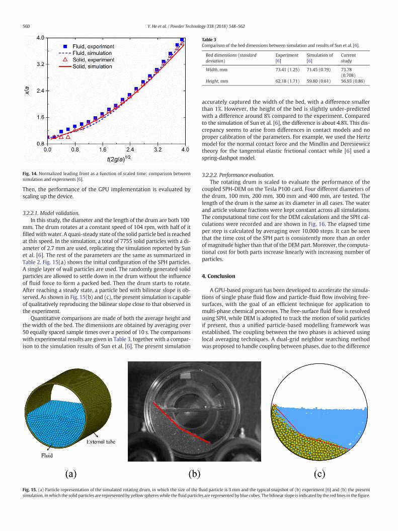
Fig. 14. Normalized leading front as a function of scaled time: comparison betweensimulation and experiments [6].

Table 3Comparison of the bed dimensions between simulation and results of Sun et al. [6].

Bed dimensions (standarddeviation)

Experiment[6]

Simulation of[6]

Currentstudy

Width, mm 73.41 (1.25) 71.45 (0.79) 73.78(0.708)

Height, mm 62.18 (1.71) 59.80 (0.61) 56.93 (0.86)

560 Y. He et al. / Powder Technology 338 (2018) 548–562

Then, the performance of the GPU implementation is evaluated byscaling up the device.

3.2.2.1. Model validation.In this study, the diameter and the length of the drum are both 100

mm. The drum rotates at a constant speed of 104 rpm, with half of itfilledwithwater. A quasi-steady state of the solid particle bed is reachedat this speed. In the simulation, a total of 7755 solid particles with a di-ameter of 2.7 mm are used, replicating the simulation reported by Sunet al. [6]. The rest of the parameters are the same as summarized inTable 2. Fig. 15(a) shows the initial configuration of the SPH particles.A single layer of wall particles are used. The randomly generated solidparticles are allowed to settle down in the drum without the influenceof fluid force to form a packed bed. Then the drum starts to rotate.After reaching a steady state, a particle bed with bilinear slope is ob-served. As shown in Fig. 15(b) and (c), the present simulation is capableof qualitatively reproducing the bilinear slope close to that observed inthe experiment.

Quantitative comparisons are made of both the average height andthe width of the bed. The dimensions are obtained by averaging over50 equally spaced sample times over a period of 10 s. The comparisonswith experimental results are given in Table 3, together with a compar-ison to the simulation results of Sun et al. [6]. The present simulation

Fig. 15. (a) Particle representation of the simulated rotating drum, in which the size of the flsimulation, inwhich the solid particles are representedby yellow sphereswhile thefluid particle

accurately captured the width of the bed, with a difference smallerthan 1%. However, the height of the bed is slightly under-predictedwith a difference around 8% compared to the experiment. Comparedto the simulation of Sun et al. [6], the difference is about 4.8%. This dis-crepancy seems to arise from differences in contact models and noproper calibration of the parameters. For example, we used the Hertzmodel for the normal contact force and the Mindlin and Deresiewicztheory for the tangential elastic frictional contact while [6] used aspring-dashpot model.

3.2.2.2. Performance evaluation.The rotating drum is scaled to evaluate the performance of the

coupled SPH-DEM on the Tesla P100 card. Four different diameters ofthe drum, 100 mm, 200 mm, 300 mm and 400 mm, are tested. Thelength of the drum is the same as its diameter in all cases. The waterand article volume fractions were kept constant across all simulations.The computational time cost for the DEM calculations and the SPH cal-culations were recorded and are shown in Fig. 16. The elapsed timeper step is calculated by averaging over 10,000 steps. It can be seenthat the time cost of the SPH part is consistently more than an orderofmagnitude higher than that of the DEMpart. Moreover, the computa-tional cost for both parts increase linearly with increasing number ofparticles.

4. Conclusion

A GPU-based program has been developed to accelerate the simula-tions of single phase fluid flow and particle-fluid flow involving free-surfaces, with the goal of an efficient technique for application tomulti-phase chemical processes. The free-surface fluid flow is resolvedusing SPH, while DEM is adopted to track the motion of solid particlesif present, thus a unified particle-based modelling framework wasestablished. The coupling between the two phases is achieved usinglocal averaging techniques. A dual-grid neighbor searching methodwas proposed to handle coupling between phases, due to the difference

uid particle is 3 mm and the typical snapshot of (b) experiment [6] and (b) the presents are represented byblue cubes. The bilinear slope is indicated by the red lines in thefigure.

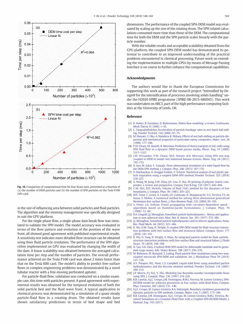
Fig. 16. Comparison of computational time for four drum sizes, presented as a function of(a) the number of DEM particles and (b) the number of SPH particles on the Tesla P100GPU card.

561Y. He et al. / Powder Technology 338 (2018) 548–562

in the size of influencing area between solid particles and fluid particles.The algorithm and the memory management was specifically designedto suit the GPU platform.

For the single phase flow, a single-phase dam break flow was simu-lated to validate the SPH model. The model accuracy was evaluated interms of the flow pattern and evolution of the position of the wavefront, all showed good agreement with published experimental results.A sensitivity test indicatesmore detailed flow structure can be obtainedusing finer fluid particle resolution. The performance of the SPH algo-rithm implemented on GPU was evaluated by changing the width ofthe dam. A linear scalability was obtained between the averaged calcu-lation time per step and the number of particles. The overall perfor-mance achieved on the Tesla P100 card was about 2 times faster thanthat on the Tesla K80 card. The model’s ability to predict free-surfaceflows in complex engineering problems was demonstrated by a noveltubular reactor with a free-moving perforated agitator.

For particle-fluid flow, validation was conducted on a similar exam-ple case, this timewith particles present. A good agreement with exper-imental results was obtained for the temporal evolution of both thesolid particle bed and the fluid wave front. A typical application tochemical process was demonstrated by a simulation of a quasi-steadyparticle-fluid flow in a rotating drum. The obtained results haveshown satisfactory predictions in terms of bed shape and bed

dimensions. The performance of the coupled SPH-DEMmodel was eval-uated by scaling up the size of the rotating drum. The SPH related calcu-lations consumedmore time than those of the DEM. The computationaltime for both the DEM and the SPH particle scales linearly with the par-ticle number.

With the reliable results and acceptable scalability obtained from theGPU platform, the coupled SPH-DEM model has demonstrated its po-tential to contribute to an improved understanding of the practicalproblems encountered in chemical processing. Future work on extend-ing the implementation to multiple GPUs by means of Message PassingInterface is on course to further enhance the computational capabilities.

Acknowledgments

The authors would like to thank the European Commission forsupporting this work as part of the research project "Intensified by De-sign® for the intensification of processes involving solids handling" un-der the H2020 SPIRE programme (SPIRE-08-2015-680565). This workwas undertaken on ARC3, part of the high performance computing facil-ities at the University of Leeds, UK.

Reference

[1] K. Hutter, B. Svendsen, D. Rickenmann, Debris flowmodeling: a review, Continuum.Mech Therm. 8 (1996) 1–35.

[2] C. Tangsathitkulchai, Acceleration of particle breakage rates in wet batch ball mill-ing, Powder Technol. 124 (2002) 67–75.

[3] M. Hussain, Y. Oku, A. Nakahira, K. Niihara, Effects of wet ball-milling on particle dis-persion and mechanical properties of particulate epoxy composites, Mater. Lett. 26(1996) 177–184.

[4] P.W. Cleary, M. Sinnott, R. Morrison, Prediction of slurry transport in SAGmills usingSPH fluid flow in a dynamic DEM based porous media, Miner. Eng. 19 (2006)1517–1527.

[5] J.W. Fernandez, P.W. Cleary, M.D. Sinnott, R.D. Morrison, Using SPH one-waycoupled to DEM to model wet industrial banana screens, Miner. Eng. 24 (2011)741–753.

[6] X. Sun, M. Sakai, Y. Yamada, Three-dimensional simulation of a solid-liquid flow bythe DEM-SPH method, J. Comput. Phys. 248 (2013) 147–176.

[7] D. Markauskas, H. Kruggel-Emden, V. Scherer, Numerical analysis of wet plastic par-ticle separation using a coupled DEM-SPH method, Powder Technol. 325 (2018)218–227.

[8] X. Wang, M. Jiang, Z.W. Zhou, J.H. Gou, D. Hui, 3D printing of polymer matrix com-posites: a review and prospective, Compos. Part B-Eng. 110 (2017) 442–458.

[9] C.W. Hirt, B.D. Nichols, Volume of fluid (Vof) method for the dynamics of freeboundaries, J. Comput. Phys. 39 (1981) 201–225.

[10] M.F. Tome, L. Grossi, A. Castelo, J.A. Cuminato, N. Mangiavacchi, V.G. Ferreira, F.S. deSousa, S. McKee, A numerical method for solving three-dimensional generalizedNewtonian free surface flows, J. Non-Newton Fluid. 123 (2004) 85–103.

[11] S. Osher, J.A. Sethian, Fronts propagating with curvature-dependent speed -algorithms based on Hamilton-Jacobi formulations, J. Comput. Phys. 79(1988) 12–49.

[12] R.A. Gingold, J.J. Monaghan, Smoothed particle hydrodynamics - theory and applica-tion to non-spherical stars, Mon. Not. R. Astron. Soc. 181 (1977) 375–389.

[13] J.J. Monaghan, Smoothed particle hydrodynamics and its diverse applications, Annu.Rev. Fluid Mech. 44 (2012) 323–346.

[14] K. Wu, D.M. Yang, N. Wright, A coupled SPH-DEMmodel for fluid-structure interac-tion problems with free-surface flow and structural failure, Comput. Struct. 177(2016) 141–161.

[15] K. Wu, D. Yang, N. Wright, A. Khan, An integrated particle model for fluid–particle–structure interaction problems with free-surface flow and structural failure, J. FluidsStruct. 76 (2018) 166–184.

[16] H. Tan, S.H. Chen, A hybrid DEM-SPH model for deformable landslide and its gener-ated surge waves, Adv. Water Resour. 108 (2017) 256–276.

[17] M. Robinson, M. Ramaioli, S. Luding, Fluid-particle flow simulations using two-way-coupled mesoscale SPH-DEM and validation, Int. J. Multiphase Flow 59 (2014)121–134.

[18] A.V. Potapov, M.L. Hunt, C.S. Campbell, Liquid-solid flows using smoothed particlehydrodynamics and the discrete element method, Powder Technol. 116 (2001)204–213.

[19] J.P. Morris, P.J. Fox, Y. Zhu, Modeling low Reynolds number incompressible flowsusing SPH, J. Comput. Phys. 136 (1997) 214–226.

[20] R.B. Canelas, A.J.C. Crespo, J.M. Dominguez, R.M.L. Ferreira, M. Gomez-Gesteira, SPH-DCDEM model for arbitrary geometries in free surface solid-fluid flows, Comput.Phys. Commun. 202 (2016) 131–140.

[21] A.J.C. Crespo, M. Gomez-Gesteira, R.A. Dalrymple, Boundary conditions generated bydynamic particles in SPH methods, Comput. Mater. Con. 5 (2007) 173–184.

[22] R.B. Canelas, J.M. Dominguez, A.J.C. Crespo, M. Gomez-Gesteira, R.M.L. Ferreira, Re-solved Simulation of a Granular-Fluid Flow with a Coupled SPH-DCDEM Model, J.Hydraul. Eng. 143 (2017).

562 Y. He et al. / Powder Technology 338 (2018) 548–562

[23] B. Ren, Z. Jin, R. Gao, Y.X. Wang, Z.L. Xu, SPH-DEMmodeling of the hydraulic stabilityof 2D blocks on a slope, J. Waterw. Port. Coast (2014) 140.

[24] A. Komoroczi, S. Abe, J.L. Urai, Meshless numerical modeling of brittle-viscous defor-mation: first results on boudinage and hydrofracturing using a coupling of discreteelement method (DEM) and smoothed particle hydrodynamics (SPH), Comput.Geosci. 17 (2013) 373–390.

[25] J.A. Anderson, C.D. Lorenz, A. Travesset, General purpose molecular dynamics simu-lations fully implemented on graphics processing units, J. Comput. Phys. 227 (2008)5342–5359.

[26] W.M. Brown, P. Wang, S.J. Plimpton, A.N. Tharrington, Implementing molecular dy-namics on hybrid high performance computers - short range forces, Comput. Phys.Commun. 182 (2011) 898–911.

[27] F. Kuznik, C. Obrecht, G. Rusaouen, J.J. Roux, LBM based flow simulation using GPUcomputing processor, Comput. Math. Appl. 59 (2010) 2380–2392.

[28] M. Januszewski, M. Kostur, Sailfish: a flexible multi-GPU implementation of the lat-tice Boltzmann method, Comput. Phys. Commun. 185 (2014) 2350–2368.

[29] C. Obrecht, F. Kuznik, B. Tourancheau, J.J. Roux, Multi-GPU implementation of thelattice Boltzmann method, Comput. Math. Appl. 65 (2013) 252–261.

[30] J.M. Dominguez, A.J.C. Crespo, D. Valdez-Balderas, B.D. Rogers, M. Gomez-Gesteira,New multi-GPU implementation for smoothed particle hydrodynamics on hetero-geneous clusters, Comput. Phys. Commun. 184 (2013) 1848–1860.

[31] Q.G. Xiong, B. Li, J. Xu, GPU-accelerated adaptive particle splitting and merging inSPH, Comput. Phys. Commun. 184 (2013) 1701–1707.

[32] J. Xu, H.B. Qi, X.J. Fang, L.Q. Lu, W. Ge, X.W. Wang, M. Xu, F.G. Chen, X.F. He, J.H. Li,Quasi-real-time simulation of rotating drum using discrete element method withparallel GPU computing, Particuology 9 (2011) 446–450.

[33] N. Govender, D.N. Wilke, S. Kok, Blaze-DEMGPU: modular high performance DEMframework for the GPU architecture, SoftwareX 5 (2016) 62–66.

[34] J.Q. Gan, Z.Y. Zhou, A.B. Yu, A GPU-based DEM approach for modelling of particulatesystems, Powder Technol. 301 (2016) 1172–1182.

[35] J.W. Zheng, X.H. An, M.S. Huang, GPU-based parallel algorithm for particle contactdetection and its application in self-compacting concrete flow simulations, Comput.Struct. 112 (2012) 193–204.

[36] Y. He, T.J. Evans, A.B. Yu, R.Y. Yang, A GPU-based DEM for modelling large scalepowder compaction with wide size distributions, Powder Technol. 333 (2018)219–228.

[37] K. Zhou, Q.M. Hou, R. Wang, B.N. Guo, Real-time KD-tree construction on graphicshardware, Acm T Graphic. (2008) 27.

[38] C. Lauterbach, Q. Mo, D. Manocha, gProximity: hierarchical GPU-based operationsfor collision and distance queries, Comput. Graph. Forum 29 (2010) 419–428.

[39] S. Pabst, A. Koch, W. Strasser, Fast and scalable CPU/GPU collision detection for rigidand deformable surfaces, Comput. Graph. Forum 29 (2010) 1605–1612.

[40] T.B. Anderson, R. Jackson, A. Fluid Mechanical, Description of fluidized beds, Ind.Eng. Chem. Fundam. 6 (1967) 527.

[41] Y. He, T.J. Evans, Y.S. Shen, A.B. Yu, R.Y. Yang, Discrete modelling of the compactionof non-spherical particles using a multi-sphere approach, Miner. Eng. 117 (2018)108–116.

[42] Y. He, T.J. Evans, A.B. Yu, R.Y. Yang, DEM investigation of the role of friction inmechanical response of powder compact, Powder Technol. 319 (2017)183–190.

[43] Y. He, Z. Wang, T.J. Evans, A.B. Yu, R.Y. Yang, DEM study of the mechanical strengthof iron ore compacts, Int. J. Miner. Process. 142 (2015) 73–81.

[44] W. Dehnen, H. Aly, Improving convergence in smoothed particle hydrodynamicssimulations without pairing instability, Mon. Not. R. Astron. Soc. 425 (2012)1068–1082.

[45] J.J. Monaghan, Simulating free-surface flows with SPH, J. Comput. Phys. 110 (1994)399–406.

[46] J.J. Monaghan, SPH without a tensile instability, J. Comput. Phys. 159 (2000)290–311.

[47] J.K. Chen, J.E. Beraun, T.C. Carney, A corrective smoothed particle method for bound-ary value problems in heat conduction, Int. J. Numer. Methods Eng. 46 (1999)231–252.

[48] P.W. Randles, L.D. Libersky, Smoothed particle hydrodynamics: some recent im-provements and applications, Comput. Method Appl. M 139 (1996) 375–408.

[49] R.A. Dalrymple, O. Knio, SPH modelling of water waves, Coastal Dynamics '01: Pro-ceedings, 2001 779–787.

[50] M. Gomez-Gesteira, D. Cerqueiroa, C. Crespoa, R.A. Dalrymple, Green waterovertopping analyzed with a SPH model, Ocean Eng. 32 (2005) 223–238.

[51] A.J.C. Crespo, M. Gomez-Gesteira, R.A. Dalrymple, 3D SPH Simulation of large wavesmitigation with a dike, J. Hydraul. Res. 45 (2007) 631–642.

[52] S. Adami, X.Y. Hu, N.A. Adams, A generalized wall boundary condition for smoothedparticle hydrodynamics, J. Comput. Phys. 231 (2012) 7057–7075.

[53] R.D. Mindlin, H. Deresiewicz, Elastic Spheres in Contact under Varying ObliqueForces, J. Appl. Mech.-T Asme 20 (1953) 327–344.

[54] Y.C. Zhou, B.D. Wright, R.Y. Yang, B.H. Xu, A.B. Yu, Rolling friction in the dynamicsimulation of sandpile formation, Phys. A 269 (1999) 536–553.

[55] D. Shepard, A two-dimensional interpolation function for irregularly-spaced data,Proceedings of the 1968 23rd ACM National Conference, ACM 1968, pp. 517–524.

[56] S. Ergun, Fluid flow through packed columns, Chem. Eng. Prog. 48 (1952) 89–94.[57] C.Y. Wen, Y.H. Yu, Mechanics of fluidization, Chem. Eng. Prog. Symp. Ser. 62 (1966)

100–111.[58] J. Hoberock, N. Bell, Thrust: a C++ Template Libaray for CUDAavailable from:

https://github.com/thrust/thrust.[59] H.P. Zhu, Z.Y. Zhou, R.Y. Yang, A.B. Yu, Discrete particle simulation of particulate sys-

tems: theoretical developments, Chem. Eng. Sci. 62 (2007) 3378–3396.[60] S.Koshizuka, Y. Oka, H. Tamako, A Particle Method for Calculating Splashing of In-

compressible Viscous Fluid, American Nuclear Society, Inc., La Grange Park, 1L(United States), 1995.

[61] J.C. Martin, W.J. Moyce, An experimental study of the collapse of liquid columns on arigid horizontal plane 4, Philos. Trans. R Soc. S-A 244 (1952) 312–324.

[62] D.L. Browne, B.J. Deadman, R. Ashe, I.R. Baxendale, S.V. Ley, Continuous flow pro-cessing of slurries: evaluation of an agitated cell reactor, Org. Process. Res. Dev. 15(2011) 693–697.

[63] G. Gasparini, I. Archer, E. Jones, R. Ashe, Scaling up biocatalysis reactions in flow re-actors, Org. Process. Res. Dev. 16 (2012) 1013–1016.

[64] Y. He, A.E. Bayly, A. Hassanpour, Coupling CFD-DEM with dynamic meshing: a newapproach for fluid-structure interaction in particle-fluid flows, Powder Technol. 325(2018) 620–631.