a guide to solidthinking compose · 2018-05-04 · will find yourself at a higher level of...

i

A GUIDE TO solidThinking

COMPOSE For Beginners and Experienced Users

Author- Sijo George

Altair Engineering

Bangalore

ii

ABOUT THE TUTORIAL

COMPOSE is a programming language developed by Altair Engineering. It started out as a matrix programming language.

This tutorial gives you a complete introduction of COMPOSE programming language.

Problem-based COMPOSE examples have been given in simple and easy to make your learning

fast and effective.

AUDIENCE

This tutorial has been prepared for the beginners and experienced users to help them

understand basic to advanced functionality of COMPOSE. After completing this tutorial you

will find yourself at a higher level of expertise in using COMPOSE from where you can take

yourself to next levels.

PREREQUISITES

We assume you have a little knowledge of any computer programming and

understand concepts like variables, constants, expressions, statements, etc. If you have done

programming in any other high-level language like C, C++, Java or MATLAB, then it will be very

much beneficial in learning COMPOSE.

iii

Contents

About the Tutorial…………………………………………………………………………………………...ii

Audience………………………………………………………………………………………….……………...ii

Prerequisites…………………………………………………………………………………………………...ii

Contents………………………………………………………………………………………………………….iii

1. GENERAL USAGE AND THE USER INTERFACE………………………………...1

1.1 Ability in Computational mathematics……………….…...………………………..1

1.2 The Environment………………………………………………………………………………1

1.2.1 File Toolbar…………………………………………………………………….2

1.2.2 Debugging Toolbar…………………………………………………………2

1.2.3 Project Browser……………………………………………………………..2

1.2.4 Editor Window……………………………………………………………….2

1.2.5 Command Window…………………………………………………………2

1.2.6 File Browser……………………………………………………………………2

1.2.7 Command History and Variable Browser Window…………..2

1.2.8 Property Editor………………………………………………………………3

1.2.9 Help Options………………………………………………………………….3

1.2.10 Auto Complete Feature……………………………………………..…4

1.2.11 Case Sensitivity & First Index…………………………………………4

2. COMMANDS AND DATA TYPES

2.1 General Commands..……………………………………………………………………….5

2.2 System Commands…………………………………………………………………………..9

2.3 Data Types…………………………………………..…………………………………..…...13

2.3.1 Strings…………………………………………………………………………13

2.3.2 Doubles……………………………………………………………………….13

iv

2.3.3 Booleans……………………………………………………………………..15

2.3.4 Complex Numbers……………………………………………………….14

2.3.5 Matrices………………………………………………………………………15

2.3.6 Cells…………………………………………………………………………….17

2.3.7 Structures……………………………………………………………………18

2.4 Operators…………….…………………………..………………………………………....20

3. COMMANDS FOR MATH AND CURVE FITTING……………………….…………………..23

3.1 General Math………………………………………………………………………………..23

3.2 Trigonometry………………………………………………………………………………..29

3.3 Curve Fitting………………………………………………………………………………....29

4. MATRICES AND VECTORS……………………………………………………………………………33

4.1 Matrix & Linear Algebra Commands……………..……………………………….33

5. PLOT ATTRIBUTES AND HANDLE MANAGEMENT…………………………………………46

5.1 Window Management…………………………………………………………………..46

5.2 Plot Types……………………………………………………………………………………..48

5.3 Line Attributes………………………………………………………………………………54

5.4 Handle Management and Plot Attributes……………………………………..55

6. LOGIC AND LOOPING………………………………………………………………………………….57

6.1 General Commands……………………….……………………………………………57

6.2 Comparison Commands………………………………………………………………58

6.3 ‘Is’ Check Commands………….....……………………………………………………59

7. FUNCTIONS AND DEBUGGING…….………………………………………………………………61

7.1 Functions…………………………………………………………………………………..…61

v

7.1.1 Syntax to Define a Function…………………………………………….61

7.1.2 Syntax to call a Function…………………………………………………62

7.1.3 Scoping………………………………………………………………………….63

7.1.4 Storing Functions in File………………………………………………….63

7.1.5 Commands related to functions……………………………………..64

7.2 Debugging……………………………………………………………………………………66

7.2.1 Watch Window……………………………………………………………….68

7.2.2 Call Stack Window…………………………………………………………..68

8. STRINGS, FILES AND I/O………………………………………………………………………………69

8.1 Format Specifiers………………………………………………………………………….69

8.2 General Commands for string Operation………………………………………71

8.3 Files & I/O…………………………………………………………………………………….73

8.4 Hypergraph………………………………………………………………………………….75

9. INTERFACING WITH OTHER LANGUAGES…………………………………………………….78

10. ADD CUSTOM/USER DEFINED FUNCTIONS TO COMPOSE USING C/C++ CODES FROM VISUAL STUDIO 2015 IN WINDOWS PLATFORM………………………..79

11. ADD CUSTOM/USER DEFINED FUNCTIONS TO COMPOSE USING C/C++ CODES IN LINUX PLATFORM……………………………………………………………………………84

12. HIGHER LEVEL COMMANDS………………………………………………………..……………89

12.1 Signal Processing……………………………………………………………………….89

12.1.1 Generation of basic Signals……………………………………………89

12.1.2 Impulse Response of a given system………………………………93

12.1.3 Linear Convolution of two sequences……………………………95

vi

12.1.4 Linear Convolution using DFT/IDFT……………………………….97

12.1.5 Circular Convolution of two sequences…………………………98

12.1.6 Auto Correlation of a given sequence…………………………101

12.1.7 Design of Butterworth IIR Filter…………………………………..103

12.1.8 Design of FIR Low Pass Filter………………………………………104

12.1.9 Chebyshev Type-1 Analog Filter…………………………………106

12.1.10 Chebyshev Type-2 Analog Filter………………………………108

12.1.11 Generation of AM, FM and PWM waveforms……………110

12.2 Statistics…………………………………………………………………………………...114

12.2.1 PDF and CDF of 2 Distribution………………………………….114

12.2.2 Mean, Variance and Standard Deviation…………………..115

12.2.3 Linear Regression……………………………………………………..115

12.2.4 PDF and CDF using Poisson’s Distribution………………….116

12.2.5 Mass spring Damper system DE solving…………………….117

12.2.6 Vander Pol’s Oscillator Differential Equation…………….118

12.3 Control System………………………………………………………………………..120

12.3.1 Step Response of Second Order System…………………….120

12.3.2 Effect of P, PI, PD and PID Controller…………………………125

12.3.3 Bode Plot and Nyquist Plot……………………………………….130

12.3.4 Root Locus……………………………………………………………….134

12.3.5 Lag, Lead & Lead-Lag Compensator using Bode Plot….138

12.3.6 Real Time Control of Inverted Pendulum…………………..152

12.4 Optimization and solving…………………………………………………………155

12.4.1 Non Linear Programming………………………………………….155

12.4.2 Genetic Algorithm…………………………………………………….157

12.5.3 Non Linear Equality Constraints Optimization…………..158

12.5 GUI Creation in Compose…………………………………………………………164

12.5.1 Step Response using a slider……………………………………..164

vii

12.5.2 Step Response/Bode Plot/Root Locus using GUI………166

12.5.3 Signal Operations using GUI………………………………………173

12.6 UDP Communication between Embed and Compose………………183

12.7 Interrupt Based Serial Communication in Compose…………………192

12.7.1 GPIO & Arduino Part…………………………………………………193

12.7.2 Visual Studio Part………………………………………………….…197

1

1. GENERAL USAGE AND USER INTERFACE

Compose’s Integrated Development Environment (IDE) offers two modes: Authoring

and Debugging. The Authoring mode is active by default and is used to create, edit and

execute scripts. IDE supports OML (solidThinking Compose Language) and Tcl languages in the

latest release. Editing, executing and debugging of scripts is made easy with additional tools

such as a Project browser, a Command History widget or a Variable Browser.

The Debug mode enables you to debug scripts. The debugger must be turned ON (use

F5) on a given file. When turned on, additional components such as watch window are added

to the environment. They are removed when the debugger is stopped.

1.1 COMPOSE’s Power of Computational Mathematics

Compose can be used in every facet of computational mathematics. Following are some

applications where it can be used:

CAE data processing (any industry)

Test data Processing (any industry)

Signal Processing

Statistics

General Math Processing

File I/O

Plotting

Various other special functions

1.2 The Environment

The below figure shows the solidThinking Compose in authoring mode. The description of

the various toolbars in the default authoring mode is described below.

Figure 1.2.a: sT Compose in Authoring Mode

2

1.2.1 File Toolbar

It helps in creating new opening and saving script files.

1.2.2 Debugging Toolbar

It helps in evaluating and debugging the current script file.

1.2.3 Project Browser

It displays the current session content and open files added to the project. It also displays

the open plots.

1.2.4 Editor Window

It allows users to create or open files for authoring and execution. It supports syntax

highlighting, smart indentation, collapsible sections, bookmarking and displaying line

numbers.

1.2.5 Command Window

It allows execution of solidThinking Compose or Tcl language commands. Separate

command windows are available for different languages which are accessible from View

menu. It also displays print commands from evaluated scripts in editor.

1.2.6 File Browser

File browser allows for browsing folder contents, adding new files and deleting existing

files. The displayed list can be filtered by file types, or by matching a pattern.

1.2.7 Command History & Variable Browser Window

It displays all commands processed by date. It allows for quick execution of commands.

Double clicking executes the selected command and we can also drag and drop commands

into the command window or editor window.

Figure 1.2.7.a: sT Compose Command History & Variable browser window

Variable browser lists all the variables in the session. It identifies the variables by their

value, type and scope of the function. We can delete or modify the variables. We can also

open a matrix in the matrix editor to modify a matrix.

3

1.2.8 Property Editor

It shows or hide the different panels. We can also dock or undock different panels from

property editor.

1.2.9 Help Options

We can select objects with the right mouse button which allows help access to that

object from within the editor or command windows. It also contains other options depending

on the object and window.

Figure 1.2.9.a: sT Compose options on help

General help can be accessed through File--->Help menu

Figure 1.2.9.b: sT Compose General Help Window

4

1.2.10 Auto Complete feature

Compose has an auto-complete feature for functions and arguments. When you type a

particular functions, it automatically lists all related functions. To quickly open files, compose

includes a ability to drag and drop from the file browser to the editor windows.

Figure 1.2.10.a: sT Compose Auto Complete features

1.2.11 Case Sensitivity & First Index

solidThinking Compose is case sensitive. Ending a command line with ‘;’ prevents

compose from echoing the result of the command in the command window.

Figure 1.2.11.a: sT Compose Case sensitive nature

‘1’ is the first index of an element in an array of matrix component.

Figure 1.2.11.b: sT Compose first index digit in an array

5

2. COMMANDS AND DATA TYPES

Over 500 commands and functions are included in solidThinking Compose. It includes

General Commands

System Commands

Mathematical Operators

Mathematical functions

Logical and Looping operators and commands

Plotting commands

File I/O and CAE reader commands

2.1 General Commands

The following general commands are explained in detail.

funclist

clear

clc

close/close all

who

whos

date

tic/toc

clock

pause

funclist

This command generates a list of all commands supported by solidThinking Compose.

Figure 2.1.a: sT Compose’s list of functions

6

clear

This command clears all variables from memory. Example is given below.

Figure 2.1.b: sT Compose’s ‘clear’ command

clc

This command empties out the display of the command window. Example is given below.

Figure 2.1.c: sT Compose’s ‘clc’ command

close/close all

This command closes one or all plots. Example is given below.

Figure 2.1.d: sT Compose’s ‘close all’ command

7

Starting a script with the following three commands is a good programming practise. Example

is given below.

Figure 2.1.e: sT Compose’s editor window

who

This command lists all variables in the current scope. Example is given below.

Figure 2.1.f: sT Compose’s ‘who’ command

whos var

This command list all variable names in the current scope and the variables

size/bytes/class. If a single variable name for ‘var’ is given, the function ‘whos’ will list only

the specified variable information. Example is given below.

Figure 2.1.g: sT Compose’s ‘whos’ command

8

date

This command shows the current date. Example is given below.

Figure 2.1.h: sT Compose’s ‘date’ command

tic/toc

This command calculates the time between the tic command is executed and toc

command execution. Example is given below.

Figure 2.1.i: sT Compose’s ‘tic/toc’ command

clock

This command shows todays date and time as a vector which will be in the form of year,

month, day, hour minute and second and it will be in 24 hr clock. Example is given below.

Figure 2.1.j: sT Compose’s ‘clock’ command

pause

This command pause the process for the given ‘n’ seconds. Example is given below.

Figure 2.1.k: sT Compose’s ‘clock’ command

9

2.2 System Commands

System commands let you perform some of the operating system commands from

within the context of solidThinking Compose.

path(‘string’, ‘string’, ‘…’)

path command with zero arguments lists the current path that solidThinking

Compose would use for searching the path. We can replace the path with through N

arguments as shown in the example below.

Figure 2.2.a: sT Compose’s ‘path’ command

add path(‘string’, ‘string’, ‘…’)

This command appends the argument list to the current search path list. The old path

is searched first followed by the new directories specified by the ‘addpath’ command.

Example is given below.

Figure 2.2.b: sT Compose’s ‘addpath’ command

rmpath(‘string’, ‘string’, ‘…’)

This command removes the directories specified from the current search path.


Figure 2.2.c: sT Compose’s ‘rmpath’ command

10

pwd

This command lists the present working directory. The ‘pwd’ command list the current

working directory where solidThinking Compose will write/read files to/from that are not

specified with an absolute or relative path. The value of this command is that same value

specified at the top of the File Browser window in the solidThinking Compose GUI. Example is

given below.

Figure 2.2.d: sT Compose’s ‘pwd’ command

dir

This command lists the files present in the working directory of MS DOS windows.


Figure 2.2.e: sT Compose’s ‘dir’ command

cd string/ chdir (‘string’)

This command changes the present working directory. Please not ‘.’ Is the current

directory and ‘..’ is the directory directly above the current working directory. Also please

note that the working directory in the file browser window updates to the directory specified

in the cd/chdir commands. Example is given below.

Figure 2.2.f: sT Compose’s ‘cd/chdir’ command

11

mkdir string/ mkdir(‘string’)

This command adds a new directory in the current directory. The return value of the

function is an integer. 1 implies the directory is successfully created. 0 implies error occurred

in creating directory. Example is given below.

Figure 2.2.g: sT Compose’s ‘mkdir’ command

rmdir string/ rmdir (‘string’)

This command remove a directory in present working directory. The return value of

the function is an integer. 1 implies successfully removed the directory and 0 implies error in

removing the directory. Example is given below.

Figure 2.2.h: sT Compose’s ‘rmdir’ command

12

getenv string / getenv (‘string’)

This command acquire the contents of an environment variable. The function return

an empty string if the environment variable does not exist. Example is given below.

Figure 2.2.i: sT Compose’s ‘getenv’ command

setenv string / setenv (‘string’, ‘string’)

This command sets or creates the solidThinking compose environment variable

identified in the first string argument to the second string argument. The environment

variables created in sT compose only apply to the current solidThinking compose session.


Figure 2.2.j: sT Compose’s ‘setenv’ command

system (‘string’)

This command executes an operating system command in MS DOS/Windows

command line. Any settings changed using the ‘system’ command is permanent and will

persist after sT Compose is closed. Example is given below.

Figure 2.2.k: sT Compose’s ‘system’ command

13

2.3 Data Types

In solidThinking Compose, the different data types are

Strings

Doubles

Booleans

Complex Numbers

Matrices

Cells

Structures

2.3.1 String

A string is an array of one or more characters. sT Compose provides multiple methods

to store and retrieve data from a string. Example is given below.

I method: a=’this is a string’

II method: a=char(‘this is a string’)

View:

a(1) shows t

a(1:4) shows this

a(11:14) shows stri

length(a) shows 16 Figure 2.3.1.a: string in sT Compose

Strings are the output of many functions. Example is illustrated below.

Figure 2.3.1.b: Output as a string

2.3.2 Double

A double is any real number between positive and negative infinity. Examples are given below.

Figure 2.3.2.a: data type double in sT Compose

14

2.3.3 Complex

A complex number is any number with a real and complex component. The complex

component is represented by the character ‘i’ or ‘j’ where by definition ‘i’ or ‘j’ is equal to -

1.0. Example is illustrated below.

Figure 2.3.3.a: data type double in sT Compose

real

This function returns the real part of a complex number. Example is illustrated below.

Figure 2.3.3.b: ‘real’ function in sT Compose

imag

This function returns the imaginary part of a complex number.

Figure 2.3.3.c: ‘imag’ function in sT Compose

conj

This function returns the complex conjugate of a complex number.

Figure 2.3.3.d: ‘conj’ function in sT Compose

15

2.3.4 Boolean

A Boolean is a data member that is either only True or False. In numerical form, a zero

is False and all other values are True. Booleans are generally used in logical expressions for

script control which is covered in later chapters. Example is illustrated below.

Figure 2.3.4.a: ‘boolean’ in sT Compose

2.3.5 Matrix

A matrix is a data entity that holds N Rows X M Columns double, Boolean or character

data. If N=M, then the matrix is known as square matrix. Only two dimensional matrices are

supported in this release. Example is illustrated below.

Figure 2.3.5.a: matrix in sT Compose

Matrices with just one row or matrices with just one column are referred to as 1 row by N

columns or row vector and matrices with just one row are referred to as N rows by 1 column

or column vector. Example is illustrated below.

Figure 2.3.5.b: row vector and column vector in sT Compose

16

You can also create matrix by providing specific cell values and St Compose will setup a

minimum required matrix and fill the gaps with zeros. Example is illustrated below.

Figure 2.3.5.c: matrix generation in sT Compose

To recall values from the matrix simply provide the requested rows and columns using (r,c) or

(r,:) or (:,c) or ([range],[range]). Example is illustrated below.

Figure 2.3.5.d: matrix value recall in sT Compose

You can also populate data in matrices by referring to existing variables. Example is illustrated

below.

Figure 2.3.5.e: data gathering in matrix sT Compose

17

2.3.6 Cell

A cell is a two dimensional data structure made up of matrices or cells with different

dimensions and index lengths. Example is illustrated below.

Figure 2.3.6.a: cell in sT Compose

To assign and retrieve the data within a specific cell address use the {}. Please note the

syntax for accessing a matrix within a cell. Example is illustrated below.

Figure 2.3.6.b: data retrieval from cell in sT Compose

You can create a cell directly just by using the {}. Example is illustrated below.

Figure 2.3.6.c: creation of cell in sT Compose

18

2.3.7 Structure

A struct is the highest level data structure. The struct data structure can contain any other

data type as a ‘child’ including other struct data structures. Data members of a struct are

accessed through their associated field names using the ‘‘.’’ operator – (no quotes). For

example, if ‘x’ is a data structure and the field ‘test’ has a value of 5.5, then the command to

access the data member in sT Compose is ‘x.test’ as shown below.

Figure 2.3.7.a: ‘structure’ in sT Compose

Simply introduce a new name-value pair using the “.” Notation to create a new data member

in a struct. Example is illustrated below.

Figure 2.3.7.b: generation of structure in sT Compose

19

As shown below, a data member of a struct can also be a struct. Example is illustrated below.

Figure 2.3.7.c: structure within a structure in sT Compose

A cell can be constructed as a data member of struct. Example is illustrated below.

Figure 2.3.7.d: cell within a structure in sT Compose

20

The below example shows a structure with different data types

Figure 2.3.7.e: structure with different data types in sT Compose

2.4 Operators

Operators are commands which allow you to take actions with more than one

data members. Most are applicable to multiple kinds of data types. So this section will focus

on introducing each operator and showing a simple and more involved examples of each. The

different operators in sT Compose are

+ - * / .* ./ ^ .^

These operators are applicable for double, complex, Boolean, matrix, struct members and cell

members. Examples are illustrated below.

Figure 2.4.a: addition, multiplication and division in sT Compose

21

Dot star operation implies element wise multiplication. Example is illustrated below in the

right most figure.

Figure 2.4.b: dot star operation in sT Compose

Right array division ( ./) performs element wise division. Example is illustrated below.

Consider the matrix a=[1 2 3; 4 5 6]; and b=[7 8 9; 10 11 12]

Figure 2.4.c: right array division in sT Compose

Example for operation in cell is illustrated below.

Figure 2.4.d: Operation in cell using sT Compose

22

Operators for square matrices are given by forward divide(/) and backward divide (\). Example

is illustrated below.

Figure 2.4.e: Forward and backward division in sT Compose

List of other useful Commands

dos eps rename flintmax

delete sleep restoredefaultpath pathsep

i uplus celldisp putenv

j uminus complex rename

I copyfile cputime run

J class datenum

exit varlist disp

quit vardetail realmin

help unix realmax

23

3. COMMANDS FOR MATH AND CURVE FITTING

This section covers the following categories of built in commands:

General Math

Trigonometry

Curve Fitting

3.1 General Math

General Math includes functions and commands that are general math calculations

which provide a foundation user defined functions.

pi and e

pi and e are constants. These are illustrated below.

Figure 3.1.a: Forward and backward division in sT Compose

ceil (scalar/complex/matrix)

This command is applicable for scalar, complex and matrix data types. This command

returns the next integer greater than the given number, unless the number provided is an

integer in which case it just returns that. If the argument is complex, the function will return

the next largest integer as described above for both the real and complex parts. Example is

illustrated below.

Figure 3.1.b: ‘ceil’ command in sT Compose

24

floor (scalar/complex/matrix)

This command is applicable for scalar, complex and matrix data types. This command

returns the next integer below the given number, unless the number provided is an integer

in which case it just returns that number. If the number is complex, the function will return

the ‘floor’ for both the real and imaginary parts. Example is illustrated below.

Figure 3.1.c: ‘floor’ command in sT Compose

round(scalar/complex/matrix)

This command is applicable for scalar, complex and matrix data types. For positive

numbers, it returns the next integer above the given number in the absolute sense if the

numbers fractional part is between 0.5 and 0.999… It returns the next integer below the given

number in the absolute sense if the numbers decimal portion is decimal of n.0 to n.49999… If

the number is complex, the function will return the round value for both the real and

imaginary parts. Example is illustrated below.

Figure 3.1.d: ‘round’ command in sT Compose

25

mod (scalar/matrix, scalar/matrix)

This command divides the second argument (divisor) into the first (dividend) and returns

the remainder. If the input(s) are a matrix, the mod function is performed in each matrix

element in order. In the case of mod, it will always return a value that is the same sign as the

divisor. In the case where the divisor is 0, mod returns the dividend. Example is illustrated

below.

Figure 3.1.e: ‘mod’ command in sT Compose

rem (scalar/matrix, scalar/matrix)

This command divides the second argument (divisor) into the first (dividend) and returns

the remainder. In the case of rem, it will always return a value that is the same sign as the

dividend. If the inputs(s) are a matrix, the mod function id performed on each matrix element

in order. In case where the divisor is 0, rem returns the dividend. Example is illustrated below.

Figure 3.1.f: ‘rem’ command in sT Compose

max (scalar/complex/matrix, scalar/complex/matrix, scalar)

This command returns the largest value in the vector. If given a matrix, the function

will return a row vector with the maximum value of each respective column. If given 2

matrices, the function will find the maximum values pairwise between the two matrices.

There can be two outputs, the maximum value and the index of the maximum value for a

vector. The final argument controls which dimension to find the maximum value in a matrix.

1-along the column (default) or 2-along the row. Examples are illustrated below.

26

Figure 3.1.g: ‘max’ command in sT Compose

min (scalar/complex/matrix, scalar/complex/matrix, scalar)

This command gives the smallest value of the input vector. If given a matrix, the

function will return a row vector with the minimum value of each respective column. If given

two matrices, the function will find the minimum values pairwise between the two matrices.

There can be two outputs, the minimum values and the index of the minimum value for a

vecror. The final argument controls which dimension to find the maximum value in a matrix.

1-along the column (default) or 2 along the row. Examples are illustrated below.

Figure 3.1.h: ‘min’ command in sT Compose

abs (scalar/complex/matrix)

This command returns the absolute value of the number/vector. IF the argument is a

matrix the function will find the absolute value of each component individually. The absolute

value of a complex number or array is the square root of the sum of the squares of the

components. Example is illustrated below.

Figure 3.1.i: ‘abs’ command in sT Compose

27

sqrt (scalar/complex/matrix)

This command returns the square root of the number or if the argument is a matrix,

the function returns the square root of each individual component. The square root of a

complex number is calculated using DeMoivre’s theorem as below.

DeMoivre’s theorem for square root is given as

.2

sin2

cos

irbia where ,22 bar ,cos

r

a and

r

bsin

The sign of the imaginary part of the square root is the same as the sign of ‘b’ in the equation above.

Examples for sqrt are illustrated below.

Figure 3.1.j: ‘sqrt’ command in sT Compose

sum (scalar/complex/matrix, scalar)

This command returns the sum of the vector components in the argument. If the

argument is a matrix, the sum function will return a row vector with the sum of the

components in each column – same if the second argument is 1. If the second argument is2,

the sum function will return a column vector with the sum of the components in each row.

Example is illustrated below.

Figure 3.1.k: ‘sum’ command in sT Compose

28

log (scalar/complex/matrix)

This function returns the natural logarithm of the input values in the matrix argument.


Figure 3.1.l: ‘log’ command in sT Compose

sign (scalar/complex/matrix)

This command returns the unit sign (+/-) based on the sign of the scalar argument. If

the argument is a matri, the sign function will return the unit sign of each component of the

matrix. If the number is complex, the sign function will return the complex number divided

by the magnitude of the complex number. If the number is zero, the sign function will return

zero. Example is illustrated below.

Figure 3.1.m: ‘sign’ command in sT Compose

factor(N)

This command returns a row vector of the prime factor of the argument. If a second

output is requested, factor will return a row vector of the prime factors without repeating the

factors and a second row vector of how many times a factor is repeated. Example is illustrated

below.

29

Figure 3.1.n: ‘factor’ command in sT Compose

3.2 Trigonometric and hyperbolic built-in commands

sin acos tanh acosd atan2

cos atan asinh asind

tan sinh acosh cosd

asin cosh atanh sind

These commands returns the trigonometric results of the given function. If the argument is a

matrix, then the trigonometric function is applied to all number in the matrix individually.


Figure 3.2.a: trigonometric commands in sT Compose

3.3 Curve Fitting Commands

polyfit (x rowvec, y rowvec, N)

This command returns a vector of length N+1 with the coefficients of the polynomial

fit. The coefficients are ordered from highest order polynomial to smallest (ie N[1] is the

coefficient in front of the highest order polynomial)

30

polyval (N, x rowvec)

This command constructs a new vector which is based on the fit coefficients in N and

the supplied x data. Examples are illustrated below.

Figure 3.3.a: Curve fitting commands in sT Compose

In the below figure, blue line represents the original figure and the green line represents the

fitted curve.

Figure 3.3.b: Curve fitting commands in sT Compose

31

roots (rowvec)

This command returns the roots of the polynomial equation set to equal zero based

on a supplied set of fit coefficients in a row vector. For example, a row vector of coefficients

[2 0 -3] as an argument returns the roots of the equation 032 2 x

Figure 3.3.c: ‘root’ command in sT Compose

poly (rowvec)

This command returns the coefficients of the polynomial that has roots equal to the input

argument. Consider the equation x2-9=0. Roots are 3 and -3. Examples are illustrated below.

Figure 3.3.d: ‘poly’ command in sT Compose

polyder (rovec)

This command returns the coefficients of the polynomial that is the derivative of the

given polynomial. The input provides the coefficients of the given polynomial. Examples are

illustrated below.

0763)( 2 xxxf

066)(' xxf

Figure 3.3.e: ‘polyder’ command in sT Compose

32

polyint (rowvec)

This command returns the coefficients of the polynomial that is the integral of the

given polynomial. The input provides the coefficients of the given polynomial. The constant is

returned as a zero. Examples are illustrated below.

0763)(' 2 xxxf

073)( 23 xxxxf

Figure 3.3.f: ‘polyint’ command in sT Compose

spline ( rowvec, rowvec, rowvec)

This command returns the cubic spline interpolation based on the first two arguments

for the values in the third argument. In other words, the vector returned is the cubic spline

interpolation for the vector in the third argument based on the vectors in the first two

arguments. Example is illustrated below.

Figure 3.3.g: ‘spline’ command in sT Compose

List of other curve fitting commands

log10 vertcat pow2 cond lsqcurvefit

log2 horzcat angle length

fix times primes gcd

arg unwrap power interp1

33

4. MATRICES AND VECTORS

This section will be dealing with matrices, row vectors and column vectors. This section covers

Matrix Commands

Linear Algebra

4.1 Matrix and Linear Algebra Commands

eye

This function creates identity matrix. Example is illustrated below.

Figure 4.1.a: ‘eye’ command in sT Compose

meshgrid

This command create matrices populated with values in an array. Example is illustrated

below.

Figure 4.1.b: ‘meshgrid’ command in sT Compose

ones

This command create matrices of all ones. Example is illustrated below.

34

zeros

This command create matrices of all zeros. Example is illustrated below.

Figure 4.1.c: ‘ones and zeros’ commands in sT Compose

nan

This command creates matrices with ‘’NaN’’ (Abbreviation for ‘Not a real Number’).


inf

This command creates matrices with ‘’Inf’’. Example is illustrated below.

Figure 4.1.d: ‘nan and inf’ commands in sT Compose

true

This command creates Boolean values. Example is illustrated below.

false

This command creates Boolean values. Example is illustrated below.

Figure 4.1.e: ‘true and false’ commands in sT Compose

35

rand

This command creates random numbers. Example is illustrated below.

Figure 4.1.f: ‘true and false’ commands in sT Compose

[a, b, c] = intersect (matrix, matrix, ‘rows’)

This command returns one, two or three outputs as [a, b, c] = intersect (matrix,

matrix,’rows’). It returns the common values between the first two matrix input arguments.

If the two input arguments are vectors, the output is in the same orientation as the input

vector- row/column vector. Second output is the indices of the values returned in the first

output form the first matrix. Third output is the indices of the values returned in the first

output from the second matrix. If the ‘rows’ argument is included, intersect will treat each

row of the matrix as an individual entity. Examples are illustrated below.

Figure 4.1.g: ‘intersect’ command in sT Compose

Please note that when there is more than one common value, the value given in ’b’ and ‘c’ is

for the last instance of the common value.

[a, b, c] = union (matrix, matrix, ‘rows’)

This command returns one, two or three outputs as [a,b,c]=union (matrix,

matrix,’rows’). It returns all the elements in both the matrix input arguments in ascending

order in a non-repeated manner. If two input arguments are vectors, the output is in the same

orientation as the input vector- row/column vector. ‘b’ contains the indices in the first matrix

36

returned by ‘a’. ‘c’ contains the indices in the second matrix returned in ‘a’. If multiple

instances of value is present, the last instance will be used in both ‘b’ and ‘c’. If the ‘rows’

argument is included, union will treat each row of the matrix as an individual entity. Examples

are illustrated below.

Figure 4.1.h: ‘union’ command in sT Compose

[row, col, v] = find(matrix, n, ‘direction’)

This command returns one, two or three outputs in the form [row,

col,v]=find(matrix, n, ‘direction’). If there is one output requested, ‘find’ will return the indices

of the non-zero elements in the matrix. If the input argument ‘n’ is present, ‘find’ will return

the indices of the first ‘n’ non-zero values. The direction argument is either first or last to start

the search for non-zero indices from the first or last input matrix element. ‘first’ is taken

default. If two outputs are requested, ‘find’ will return the row and column indices of the non-

zero elements. For three outputs, ‘find’ will return the ‘row’ and ‘column’ indices plus a vector

of the non-zero values. Examples are illustrated below.

Figure 4.1.i: ‘find’ command in sT Compose

37

R=all (matrix, dim)

This command gives the output of the form R=all(matrix,dim) This command returns a

Boolean of ‘1’ (true) if all the values of the vector or columns of a matrix are non-zero

otherwise returns zero. If the ‘dim’ argument is ‘2’ then ‘all’ will return a Boolean of ‘1’ if all

the rows of the input matrix is non-zero- ‘dim’ of 1 is default. Example is illustrated below.

Figure 4.1.j: ‘all’ command in sT Compose

R = any (matrix)

This command gives the output of the form R=any(matrix) This command returns a

Boolean of ‘1’ (true) if any or the elements of a vector of the column vectors of a matrix are

non-zero. If the input argument ‘dim’ is set to 2, ‘all’ returns a Boolean of ‘1’ if any of the row

vectors of the input matrix contains non-zero values. Example is illustrated below.

Figure 4.1.k: ‘any’ command in sT Compose

[s, idx] = sort( matrix, dim, ‘ascend/descend’)

This command returns one or two outputs in the form [s, idx]=sort( matrix, dim,

‘ascend/descend’). It gives a column or row vector in ascending order. If the input argument

is a matrix, ‘sort’ will return a matrix with the individual column vectors sorted. If the ‘dim’

argument is set to ‘2’ and the input is a matrix, the output is a matrix with the row vectors

sorted in ascending order. If the last argument is ‘descend’, sort will return the column/row

vector of matrix in descending. The output ‘idx’ is the index of the row or column of the sorted

value in the original matrix or vector. Examples are illustrated below.

38

Figure 4.1.l: ‘sort’ command in sT Compose

[row, col] = size( matrix, dim)

This command returns one or two outputs in the form [row, column] = size(matrix,

dim). It returns a vector with the number of rows/columns of a row/column vector. With 1

output requested, it returns a row vector with the number of rows and column of matrix.

When 2 outputs are requested, the number of rows and columns in the input matrix is stored

as separate scalars. With ‘dim’ specified as an input argument, the number of rows for ‘dim=1’

or number of columns for ‘dim=2’. Examples are illustrated below.

Figure 4.1.m: ‘sort’ command in sT Compose

39

R=cumsum( matrix, dim)

This command gives the cumulative sum of the row or column vector – the sum of all

the values of lower index in the row/column vector. If the input is a matrix, ‘cumsum’ will

return the cumulative sum of the columns of the input vector. If the input is a matrix and

the ‘dim’ is ‘2’, the output is the cumulative sum of the rows of the input matrix- ‘dim=1’ is

the default. Examples are illustrated below.

Figure 4.1.n: ‘cumsum’ command in sT Compose

R = cumprod(matrix, dim)

This command gives the cumulative product of the row or column vector – the product

of all the values of lower index in the row/column vector. If the input is a matrix, ‘cumprod’

will return the cumulative product of the columns of the input vector. If the input is a matrix

and the ‘dim’ is 2, the output is the cumulative product of the rows of the input matrix-

‘dim=1’ is the default. Examples are illustrated below.

Figure 4.1.o: ‘cumprod’ command in sT Compose

40

[ C, ia, ib] = unique ( matrix, ‘rows’, ‘first’/’last’)

This command gives one or two or three outputs of the form [C ia ib]=unique(matrix,

‘rows’, ‘first’/’last’). The unique values of the vector/matrix in the first argument in a row/

column vector. The ‘ia’ vector relates the values in vector ‘C’ to the corresponding index in

matrix/vector ‘A’. The ‘ib’ vector relates the values in vector/matrix ‘A’ to the corresponding

index in vector ‘C’. As shown in green circles below, the third value in vector ‘ib’ is 8 and

applying that index value to vector ‘C’ produces the third value in vector ‘A’. If the input

arguments include ‘first’, the first index of repeated values is returned in vector ‘ia’. ‘last’ is

set as default. Compare the ‘ia’ vector, returned in the red circles to the ‘ia’ vector returned

in the purple circles. If ‘row’ is included in the input arguments, the unique row vectors of

matrix A are returned in matrix C.

Figure 4.1.p: ‘unique’ command in sT Compose

R = dot(scalar/complex/matrix, scalar/complex/matrix, dim)

This command gives output of the form R=dot (scalar/complex/matrix).This command

returns the dot product of two vectors, matrices or complex numbers. If 2 scalars are input,

then ‘dot’ multiplies the scalars. If the two arguments are matrices, ‘dot’ will return the dot

product of the column vectors. ‘Dot’ will return the dot product of the row vectors if ‘dim’ is

set to ‘2’. Examples are illustrated below.

41

Figure 4.1.q: dot product in sT Compose

R = cross( matrix, matrix, dim)

This command gives output of the form R=cross(matrix, matrix, dim). This command

returns the cross product of two vectors, matrices, or complex numbers. If two scalars are

input, then ‘cross’ multiplies the scalars. If the two arguments are matrices, ‘cross’ will return

the cross product of the column vectors. Cross will return the cross product of the row vectors

if ‘dim’ is set to ‘2’. The cross product only exists in 3 dimension vector space. The cross

product can also be expressed as

321

321

vvv

uuu

kji

vu

Figure 4.1.r: cross product in sT Compose

42

R = transpose (matrix, matrix)

This command gives output of the form R=transpose(matrix, matrix). This command

returns the transpose of the input matrix. Also the ‘’.’ ’’ operator will find the transpose of

the matrix. Example is illustrated below.

Figure 4.1.s: ‘transpose’ command in sT Compose

R = diag( matrix, m, n)

This command gives output of the form R=diag(matrix,m,n) This command gives the

diagonal of a matrix as a column vector. If the input is a vector and no other input arguments,

the function returns a matrix with diagonal equal to the input vector. If the input is a matrix

and ‘m’, the function will return the diagonal starting ‘m’ columns (or rows if ‘m’ is negative)

away from the first column. When the input is a vector and only the ‘m’ argument is present,

the function will create a matrix with the input vector a diagonal ‘m’ columns (or rows if ‘m’

is negative) away from the first entity. When the input is a vector with input arguments ‘m’

and ‘n’, the function will return a ‘mxn’ matrix with a diagonal equal to the input vector n –

both ‘m’ and ‘n’ should be greater than the size of the input vector. Example is illustrated

below.

Figure 4.1.t: ‘diag’ command in sT Compose

43

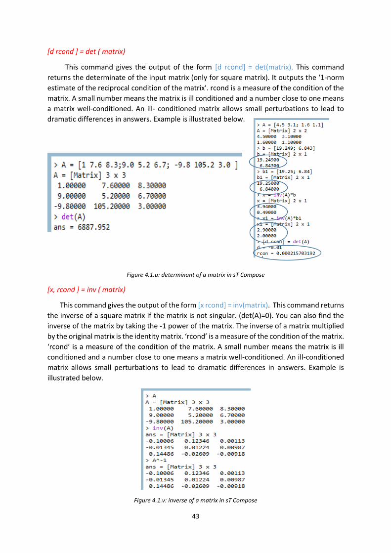
[d rcond ] = det ( matrix)

This command gives the output of the form [d rcond] = det(matrix). This command

returns the determinate of the input matrix (only for square matrix). It outputs the ‘1-norm

estimate of the reciprocal condition of the matrix’. rcond is a measure of the condition of the

matrix. A small number means the matrix is ill conditioned and a number close to one means

a matrix well-conditioned. An ill- conditioned matrix allows small perturbations to lead to

dramatic differences in answers. Example is illustrated below.

Figure 4.1.u: determinant of a matrix in sT Compose

[x, rcond ] = inv ( matrix)

This command gives the output of the form [x rcond] = inv(matrix). This command returns

the inverse of a square matrix if the matrix is not singular. (det(A)=0). You can also find the

inverse of the matrix by taking the -1 power of the matrix. The inverse of a matrix multiplied

by the original matrix is the identity matrix. ‘rcond’ is a measure of the condition of the matrix.

‘rcond’ is a measure of the condition of the matrix. A small number means the matrix is ill

conditioned and a number close to one means a matrix well-conditioned. An ill-conditioned

matrix allows small perturbations to lead to dramatic differences in answers. Example is

illustrated below.

Figure 4.1.v: inverse of a matrix in sT Compose

44

[V D]= eig(Amatrix, Bmatrix, ‘nobalance’)

This commands returns 1 or 2 outputs. V is the column vector of the Eigen value

solution. D is the diagonal matrix with the corresponding Eigen values. B is the right hand side

matrix in a generalized Eigen value problem. ‘nobalance’ disables the balancing operation

when finding the Eigen values-not recommended. Example is illustrated below.

Figure 4.1.w: ‘eig’ command in sT Compose

R=rank( matrix, tol)

This command returns the rank of the matrix. The second argument ‘tol’ is the scalar

threshold for rounding off near zero singular values. The default is the largest dimension

multiplied by eps(s) where s is the largest singular value and ‘eps’ is the spacing between two

adjacent number in a machines floating point system. The rank of a matrix is the dimension

of the vector space generated or spanned by the column vectors. Example is illustrated below.

Figure 4.1.x: ‘rank’ command in sT Compose

Eigen Vectors

Eigen Values

45

List of Other Matrix & Linear Algebra Commands

mpower lu triu numel setfield

minus chol cat expm getfield

mldivide conv permute ndims fieldnames

ind2sub conv2 pinv reshape

sub2ind cplxpair prod schur

balance diff ldivide setdiff

bitor hypot rdivide subsref

bitand mtimes mlock svd

bitxor norm munlock linspace

setxor tril repmat rmfield

46

5. PLOT ATTRIBUTES AND HANDLE MANAGEMENT

This section cover plotting and the ability to control plot attributes through handles and

commands. It includes

Window Management

Plot Types

Line Attributes

Handle Management and Plot Attributes

Plots are considered ‘objects’ in Compose. Each ‘object’ is assigned a numerical value

named a ‘handle’. Similar to object oriented programming, each ‘object’ has ‘children’.

Information and modification of an ‘objects’ & ‘children’ is accomplished through the objects

‘handle’.

5.1 Window Management

One or more plots are contained in the Compose Figure Window. When a plot is

created, a figure window is created as well. In addition, a figure window is created manually

using the ‘Figure (N)’ command. Example is illustrated below. The ‘figure (n)’ command will

activate the nth window. ‘close(n)’ command will close figure ‘n’ and ‘close all’ command

closes all figures. Examples are illustrated below.

Figure 5.1.a: Window management in sT Compose

47

subplot(R,C,N)

This command will create multiple plots within a single figure window. ‘R’ indicates the

number of rows of subplots in the window. ‘C’ denotes the number of columns of subplots in

the window. ‘N’ denotes the active plot number. The plots are number from left to right along

a row as shown in the figure below. In the example given below, a figure is created with 2

rows and 3 column of subplots. The first window is the active plot.

Figure 5.1.b: subplot command in sT Compose

To create a subplot at a location of 5th row & 2nd column, the following example is shown.

Figure 5.1.c: subplot command in sT Compose

2 1

5 4 6

3

2

4 6

3

48

5.2 Plot Types

There are different plot types in compose. The following are a list of it.

plot (2D Line) & plot3 (3D Line)

scatter (2D scatter) & ‘scatter3’ (3D Line)

‘surf’(3D surface)

‘contour’ (2D contour) & ‘countour3’ ( 3D contour)

‘waterfall’ (3D waterfall)

‘polar’ (Polar)

‘loglog’ (2D with log base 10 x & y axes)

‘bar’ (Bar)

‘area’ (Area)

h = plot(x, y, ‘fmt’, x, y, ‘fmt’, property, value)

h = plot(hAxes,…)

This command creates a 2D plot of one or more sets of data. The ‘plot(y)’ command will

plot ‘y’ values on the vertical axis against the vector index on the horizontal axis. The ‘plot(x,y)’

and ‘plot(x,y,x,y…)’ will plot the ‘x’ values on the horizontal axis and ‘y’ values on the vertical

axis. Examples are illustrated below. ‘fmt’ denotes the formatted string for the line. ‘Property’

and ‘value’ controls a graphic object in a plot. ‘hAxes’ handles the axis in the plot.

Figure 5.2.a: ‘plot’ command in sT Compose

Figure 5.2.b: ‘plot’ command in sT Compose

49

Figure 5.2.c: ‘plot’ command in sT Compose

h = scatter (x, y, …, clor, style, property, value)

h = scatter(haxes, …)

This command handles the scatter plot graphics. It creates a 2D scatter plot of the data

in vectors x and y. ‘color’ denotes the color of the scattered dots. ‘style’ denotes the style of

the scattered dots. ‘property’ and ‘value’ controls the graphic object in a plot. ‘haxes’ handles

an axis in the plot. Examples are illustrated below.

Figure 5.2.d: ‘scatter’ command in sT Compose

h = plot3(x, y, z, …, ‘fmt’, property, value)

h = plot3(hAxes, …)

This command returns the handle of the 3D line object. It creates a 3D line plot in

Cartesian space based on the three input vectors x, y, and z. If there is a complex vector, the

real part is plotted along the y-axis and imaginary part along the z-axis. If the complex input

does not have vector for x, the index of the complex number is the value plotted along the x-

axis. ‘fmt’ denotes the formatted string of the line. ‘property’ and ’value’ controls the graphic

object in a plot. ‘haxes’ handles the axis in the plot. Examples are illustrated below.

50

Figure 5.2.e: ‘plot3’ command in sT Compose

h = surf(x, y, z, …, color, property, value)

h = surf(hAxes, …)

This command returns the handle of the 3D surface object. The function will create a

surface in the form of z=f(x, y) where x and y are vectors with the same rows/columns as

matrix z. In the case where x and y are absent, the x-axis and y-axis values correspond to the

column and row indices of matrix z. Example is illustrated below.

Figure 5.2.f: ‘surf’ command in sT Compose

h = contour (z)

h = contour(x, y, z)

h = contour(hAxes, …)

This command returns the handle of the 2D surface object. The contour function will

produce a 2D contour plot. If the first argument is a matrix ‘z’, the x- axis values in the plot

are the row indices of matrix ‘z’. When the first two arguments are vectors ‘x’ and ‘y’, the

length of ‘x’ vector must be the same as the number of rows in matrix ‘z’ and the length of

the ‘y’ vector must equal the number of columns in matrix ‘x’. If the first argument is a contour

handle, the contour plot is created on the corresponding system. Example is illustrated below.

51

Figure 5.2.g: ‘contour’ command in sT Compose

h = contour3(z)

h = contour3(x, y, z)

h = contour3(haxes, ..)

This command returns the handle of the 3D surface object. The contour function will

produce a 3D contour plot. If the first argument is a matrix ‘z’, the x-axis values in the plot are

the row indices of matrix ‘z’ and the y-axis values are the column indices of matrix ‘z’. When

the first two arguments are vectors ‘x’ and ‘y’, the length of the ‘x’ vector must be the same

as the number of rows in matrix ‘z’ and the length of the ‘y’ vector must equal the number of

columns in matrix ‘x’. If the first argument is a contour handle, the contour plot is created on

the corresponding system. Example is illustrated below.

Figure 5.2.h: ‘contour3’ command in sT Compose

h = waterfall(z)

h = waterfall(x, y, z, …, color, …, property, value)

h = waterfall(hAxes)

This command returns the handle of the waterfall plot. It creates a 3D plot of a surface

by determining the 2D ‘slices’ of the surface along y-axis. If the first argument is a matrix ‘z’,

52

the x-axis values in the plot are the row indices of matrix ‘z’ and the y-axis values are the

column indices of matrix ‘z’. When the first two arguments are vectors ‘x’ and ‘y’, the length

of the ‘x’ vector must be the same as the number of rows in matrix ‘z’ and the length of the

‘y’ vector must equal the number of columns in matrix ‘x’. If the first argument is a contour

handle, the contour plot is created on the corresponding system. ‘property’ and ‘value’

denotes the property and value that controls a graphic object in a plot. ’haxes’ denotes the

handle of an axis in the plot. Example is illustrated below.

Figure 5.2.i: ‘waterfall’ command in sT Compose

h = polar(theta, rho, fmt, theta, rho, fmt, …)

h = polar(complex, fmt)

h = polar(hAxes, …)

This command returns the handle of the polar line. It creates a 2D polar plot of the

vectors ‘theta’ and angle in radians and ‘rho’ the radius. If a complex number is the numerical

argument, ‘polar’ will use the real part as ‘theta’ and imaginary part as ‘rho’. If an axes handle

is the first argument, polar will plot on the input handle axes. ‘fmt’ denotes the formatting

string for the line. ‘haxes’ denotes the handle of an axis in the plot. Example is illustrated

below.

Figure 5.2.j: ‘polar’ command in sT Compose

53

h = semilogy(x, y, x, y, …, fmt, property, value)

h = semilogy(hAxes, …)

This command returns a row vector of line handles. It creates a 2D plot of one or

more sets of data where the y-axis is scaled by log base10. If there is only one argument, the

command will plot the ‘y’ values on the vertical axis against the vector index on the horizontal

axis. If the first argument is an axes handle, ‘semilogy’ will plot the lines on those axes. ‘fmt’

denotes the formatting string for the line. ‘property’ and ‘value’ controls the graphic object

in a plot. ‘haxes’ denotes the handle of an axis in the plot. Example is illustrated below.

Figure 5.2.k: ‘semilogy’ command in sT Compose

h = loglog(x, y, x, y, …, fmt, property, value)

h = loglog(hAxes, …)

This command returns a row vector of line handles. It creates a 2D plot of one or more

sets of data where the both axes are scaled by log base10. If there is only one argument, the

command will plot the ‘y’ values on the vertical axis against the vector index on the horizontal

axis. If the first argument is an axes handle, ‘loglog’ will plot the lines on those axes. ‘property’

and ‘value’ controls the graphic object in a plot. ‘haxes’ denotes the handle of an axis in the

plot. Example is illustrated below.

Figure 5.2.l: ‘loglog’ command in sT Compose

54

5.3 Line Attributes

The default color of the first three lines in a plot is blue, green, and red. In a ‘format

string’ after the ‘x, y’ vector input add one of the characters above to control the line and

marker color.

Figure 5.3.a: ‘plot’ options in sT Compose

Markers are at the exact locations of the values in the ‘x’ and ‘y’ input vectors. By default, the

markers are not shown. To add marker, add one of the below characters to a plot format

string.

Figure 5.3.b: ‘plot’ options in sT Compose

55

By default, the line is solid. To change the line style, add one of the characters in the table

below to the data pair’s format string.

Figure 5.3.c: ‘plot’ options in sT Compose

List of other plotting Commands

title(‘string’) text(x,y,’string’)

xlabel(‘string’) cla(N)

ylabel(‘string’) clf(N)

legend(‘string’) hold on/off/all

line(rowvec, rowvec) grid

text(x,y,’string’) axes(rowvec)

5.4 Handle Management and Plot Attributes

Plots are considered ‘objects’ in Compose. Each ‘object’ is assigned a numerical value

named a ‘handle’. Similar to object oriented programming, each ‘object’ has ‘children’.

Information and modification of an ‘objects’ & ‘children’ is accomplished through the objects

‘handle’.

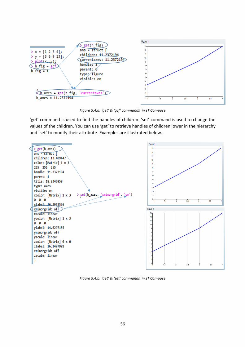
The command ‘gcf’ gives the current figure handle. ‘get’ command with no second

argument gets the handles and the values of the children of the input handle. If a property is

included in the second argument to ‘get’, the handle of the child requested is returned.


56

Figure 5.4.a: ‘get’ & ‘gcf’ commands in sT Compose

‘get’ command is used to find the handles of children. ‘set’ command is used to change the

values of the children. You can use ‘get’ to retrieve handles of children lower in the hierarchy

and ‘set’ to modify their attribute. Examples are illustrated below.

Figure 5.4.b: ‘get’ & ‘set’ commands in sT Compose

57

6. EXPRESSIONS, LOGIC AND LOOPING

This section introduce the concepts of expressions and how they are used in various logic

and looping concepts. It includes

General logic commands

Comparison commands

‘is’ check commands

6.1 General Commands

for

The ‘for’ loop is supported in solidThinking Compose using the syntax and provides the

ability to define an incremental loop. Example is illustrated below.

Figure 6.1.a: ‘for’ loop in sT Compose

The increment in ‘for’ loop doesn’t have to be an integer. Example is illustrated below.

Figure 6.1.b: ‘for’ loop in sT Compose

58

while

While loop is similar to a ‘for’ loop but this loop will continue until a condition is met to

end. Example is illustrated below.

Figure 6.1.c: ‘while’ loop in sT Compose

if/else/elseif/end

‘if/else/elseif/end’ make use of the following operators. Example is illustrated below.

== != > < >= <= & |

Figure 6.1.d: ‘if/else/elseif/end’ logic flow control in sT Compose

6.2 Comparison Commands

lt() - Perform less than comparison, equivalent to the <operator.

gt() - Perform greater than comparison, equivalent to the > operator.

59

eq() - Perform equality comparison, equivalent to the == operator.

le() - Perform less than or equal comparison, equivalent to the <= operator.

ge() - Perform greater than or equal comparison, equivalent to the >= operator.

ne() - Perform inequality comparison, equivalent to the != operator.

or() - Or operator. Used for logical operations.

and() - Perform logical conjunction, the 'and' operation.

not() - Returns the logical NOT of a. Equal to R = ~a.

Some examples are illustrated below.

Figure 6.2.a: comparison commands in sT Compose

6.3 ‘Is’ Check Commands

‘is’ check commands will return True if the entity entered is of the type that matches

the function.

Figure 6.3.a: ‘Is’check commands in sT Compose

List of ‘is’ check Commands

is axes isdir isfinite islogical ispc isstr

is bool isempty isglobal ismac isprime isstruct

is cell isequal ishandle ismatrix isreal isunix

iscellstr isequal ishold ismember isscalar isvarname

ischar isfield isinf isnan issorted isvector

iscomplex isfigure isletter isnumeric isspace

60

Real world representative Examples are given below.

Example 1

Example 2

61

7. FUNCTIONS AND DEBUGGING

This section introduces you about the functions and debugging tools in solidThinking

Compose.

Functions

Debugging

7.1 Functions

Functions are relatively small programs that use a combination of the commands

presented to achieve a specific purpose. Functions can be designed to take in ‘arguments’

when called and can be designed to return information to its calling context. Functions can

be stored on files and accessed by scripts outside the file where the function is stored.

7.1.1 Syntax to Define a Function

Example 1

Example 2

Example 3

“function” name of return variable name of function

Definition must contain an end statement

arguments to be passed in

62

7.1.2 Syntax to call a Function

Example 1

This function uses the value input passed in to assign a discrete value to W.

Varible to assign result to (does not have to match the name inside the function

function name

Argument(s). Can be an expression. Must match the expected type

63

Example 2

This function returns a vector of data.

7.1.3 Scoping

Variables which are defined inside a function are valid only within that function. This is

known as having ‘local scope’. Although not typically a good practice, variables declared

outside the function with a global statement can be accessed inside the function. Example is

illustrated below.

7.1.4 Storing Functions in Files

The typical use of functions is that they will be defined in one file but used by other files,

or the command window. The recognition of the functions is based on the path command

that was listed in the second chapter ‘Commands & data types’.

64

7.1.5 Commands applicable for functions

There are several commands that apply to functions as shown below.

builtin(arg1, arg2,…)

This command is used in the case where you have overloaded a function that also exists

in the core product, you can access the function in the core product using this command.


Figure 7.1.5.a: ‘builtin’ command in sT Compose

cellfun(‘func’, cell)

This command calls the function ‘func’ as many times as there are entries in cell,

each time using a single cell entry.

Figure 7.1.5.b: ‘cellfun’ command in sT Compose

error(‘string’); warning(‘string’)

This command echo’s a string in the user defined context. The string also provides

information about the function where it is being called from. Example is illustrated below.

65

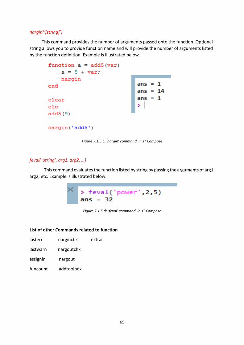
nargin(‘[string]’)

This command provides the number of arguments passed onto the function. Optional

string allows you to provide function name and will provide the number of arguments listed

by the function definition. Example is illustrated below.

Figure 7.1.5.c: ‘nargin’ command in sT Compose

feval( ‘string’, arg1, arg2, …)

This command evaluates the function listed by string by passing the arguments of arg1,

arg2, etc. Example is illustrated below.

Figure 7.1.5.d: ‘feval’ command in sT Compose

List of other Commands related to function

lasterr narginchk extract

lastwarn nargoutchk

assignin nargout

funcount addtoolbox

66

7.2 Debugging

The most common use of the product is to develop scripts and run them. This is where

the solidThinking Compose Debugging capability can be an essential tool.

Figure 7.2.a: ‘Debugging toolbar’ in sT Compose

When you invoke the debugging mode, additional windows will appear to assist with the

debugging process (they can be turned off in View menu). The additional windows appearing

during debugging mode is illustrated below.

Figure 7.2.b: Additional windows during debugging mode in sT Compose

67

Break points are central to debugging as they enable you to stop a script at any point and

monitor the script output and internal variables. You can add/manage breakpoints through

the debug menu or context menu’s in the edit area or the debug window shown below.

Figure 7.2.c: Adding break point in sT Compose

Example

This button is known as ‘step over’ which is used to execute next line. Arrow in

margin indicates the movement to next point.

This button is known as ‘continue’ which is used to resume execution until the next

breakpoint

This button is known as ‘step Into’ which is used to enter a function.

Break Points

68

This button is known as ‘Step Out’ which is used to exit a function and moves to point

where function was called.

This button is known as ‘Step Until’ which is used to executes until line where the

cursor is located.

7.2.1 Watch Window

Figure 7.2.1.a: Watch Window in debugging mode

The watch window enables you to watch values of variables in real time. The values will

update as the script moves forward. As shown in the figure below, you can add variables in a

couple of ways. One is to highlight and drag from the edit window. Another is to type in the

variable where it says ‘click to add new item’. The variable can be overridden in the watch

window and the value will hold until the script overloads that new value.

Figure 7.2.1.b: To Add and remove variables in Watch Window

7.2.2 Call Stack Window

Figure 7.2.2.a: Call Stack Window in debugging mode

The Call Stack gives you the context of the breakpoint in terms of functions that have

been called to that point. For example if function A calls function B and B calls C, when your

breakpoint in C is hit, you will see a call stack showing main, A, B, C in that order.

Figure 7.2.2.b: Call Stack operation in debugging mode

69

8. STRINGS, FILES AND I/O

Strings are fundamental and important entities in programming. Strings are a series

of characters and provide a mechanism for a script to communicate with the user or files.

Strings are often constructed with a set of given characters along with utilizing the values of

variables within the program. When working with strings, control of formatting is important.

In solidThinking Compose, literal strings are denoted using the single quote (next to the Enter

button on typical keyboard).

Figure 8.a: To print a string in sTCompose

8.1 Format Specifiers in sTCompose

When printing a string to the screen or file there are a variety of format specifiers to choose

from:

%s %N.ns

%d %Nd

%f %N.nf

%e %N.ne

%g %N.ng

%s (%N.ns)

This is used to format a string. The ‘N’ designates total columns. The string will be

written right justified in that set of columns. The ‘n’ defines how many of the characters of

the given string will be written (again right justified)

Figure 8.1.a: string operation in sT Compose

%d

This format is to create an integer. The N designates the total columns. The integer will

be right justified. This format specifier has no ‘n’.

Figure 8.1.b: string operation in sT Compose

70

If a real is given with a %d then it will be truncated.

Figure 8.1.c: string operation in sT Compose

%f (%N.nf)

This format is to format a float or real. The N designates total columns. The number will

be written right justified in that set of columns. The ‘n’ defines how many values after the

decimal will be shown.

Figure 8.1.d: string operation in sT Compose

%e (%N.ne)

This format is used to create an exponential based format. The N designates total

columns. The number will be written right justified in that set of columns. The ‘n’ defines how

many values after the decimal will be shown. The exponent will show in two columns.

Figure 8.1.e: string operation in sT Compose

%g (%N.ng)

This format is used where a number less than one million will print using ‘f’ format and

numbers one million or more will print in e-format. This is most useful when you don’t know

the magnitude of a value ahead of time but want to print smaller numbers in ‘f’ format.

The N designates total columns. The number will be written right justified in that set of

columns. The n defines how many values after the decimal will be shown. The exponent will

show in tow columns in the case where it writes e format.

71

Figure 8.1.f: string operation in sT Compose

8.2 General Commands for string Operation

stcmp(‘string1’, ‘string2’)

This command compares string1 and string2 and if they are exactly the same, it returns 1.

Otherwise it returns 0.

Figure 8.2.a: ‘strcmp’ command in sT Compose

strcat(‘string1’, ‘string2’)

This command appends each subsequent string to form one single string. You have to

insert blank spaces where desired. Example is illustrated below.

Figure 8.2.b: ‘strcat’ command in sT Compose

strfind(‘string1’, ‘string2’)

This command looks to find instances of string2 inside of string1. A vector will be returned

with each value representing the character position in string1 where string2 begins. Example


Figure 8.2.c: ‘strfind’ command in sT Compose

72

strsplit(‘string’, ‘string’)

This command will break a string at the spaces and store each word in a position in a cell.

You can however use an optional delimiter argument. Example is illustrated below.

Figure 8.2.d: ‘strsplit’ command in sT Compose

strjoin(cell, ‘string’)

The cell data members of this command should be strings. By default this command will

join all the cell members with as space between each. The optional string argument can

replace the space as the item put between each data member. Example is illustrated below.

Figure 8.2.e: ‘strjoin’ command in sT Compose

strtrim(‘string’)

This command trims the spaces on either side of the given string. Example is illustrated

below.

Figure 8.2.f: ‘strtrim’ command in sT Compose

lower (‘string’); tolower(‘string’)

upper(‘string’); toupper(‘string’)

This command modify the given string to be all lower or upper case.

Figure 8.2.g: ‘strtrim’ command in sT Compose

73

sprintf( ‘format’, number)

This command returns the given number as a string using the format specifier. Example


Figure 8.2.h: ‘sprintf’ command in sT Compose

8.3 Files & I/O

This section introduces you about reading from files and writing to files which is one of

the most important capabilities of sT Compose. There are two categories of I/O.

General

Usage of Altair’s data file readers & writers (same as those in HyperGraph)

8.3.1 General I/O

General I/O consists of four steps

Open file in either read, write or read/write

Read/write data to/from file

ASCII & Binary

Close file

fopen ( ‘filename’, ‘intent’)

File name is the name of the file you are opening to read from or write to or both. Intent

is to designate if you are reading, writing or both. Valid options for intent include r, w, a, r+,

w+, a+.

r-----> Open existing file for reading

w-----> Open existing or new for writing, discard any contents already in file

a------> Open existing or new for writing, append to contents already in file

r+ ----> Open existing file for reading and writing

w+ ----> Open existing or new for reading & writing, discard contents already in file

a+ ----> Open existing or new for reading & writing, append to contents already in file.

74

fprintf( fid, ‘string’)

This command is used to write information to a file using the same string formatiing as

discussed earlier in section 8.1. fid is the file id that was returned from the fopen command

fclose(fid)

This command is used to close the file such that all contents written to it are available

to users.

Examples using w

Figure 8.3.1.a: option ‘w’ for ‘fopen’ command in sT Compose

Example using a

The use of \n is to ensure the next text is written on a new line (typically you would put the

\n at the end of the previous line).

Figure 8.3.1.b: option ‘a’ for ‘fopen’ command in sT Compose

fgets(fid)

This command reads the next line in a file as one string. Example is illustrated below.

Figure 8.3.1.c: ‘fgets’ command in sT Compose

75

A string can be converted to number in the following way. The below example shows how to

read lines and turning them to numbers.

Figure 8.3.1.d: conversion of string to number in sT Compose

The below example shows how to read a line with several values and storing those in

individual cells.

Figure 8.3.1.e: conversion of string to number in sT Compose

8.4 HyperGraph

There are several commands which can be leveraged to import data from files with

formats that HyperGraph can read (examples include most CAE solvers on the market). When

HyperGraph readers are used, they bin the data from the file into the following groups where

each group has the ‘children’ shown below it:

Subcase

Type

Request

Component

76

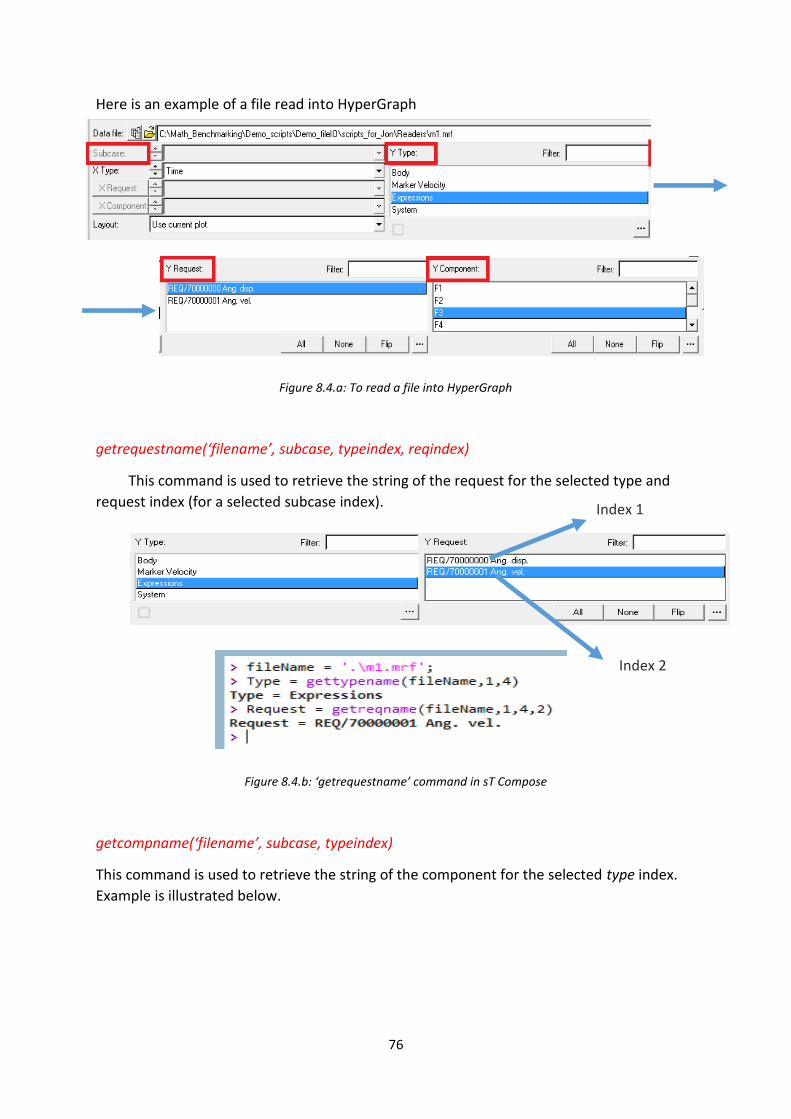
Here is an example of a file read into HyperGraph

Figure 8.4.a: To read a file into HyperGraph

getrequestname(‘filename’, subcase, typeindex, reqindex)

This command is used to retrieve the string of the request for the selected type and

request index (for a selected subcase index).

Figure 8.4.b: ‘getrequestname’ command in sT Compose

getcompname(‘filename’, subcase, typeindex)

This command is used to retrieve the string of the component for the selected type index.


Index 1

Index 2

77

Figure 8.4.c: ‘getcompname’ command in sT Compose

readvector(‘filename’, subcase, typeindex)

This command is used to retrieve an array of values from the given filename for its

corresponding type/request/component.

Figure 8.4.d: ‘readvector’ command in sT Compose

List of Commands to import data using HG readers

readvector getreqlist

getsubcasename getreqindex

getsubcaselist getcompname

getsubcaseindex getcompindex

gettypename gettotalsubcases

gettypelist getfilteredcomplist

gettypeindex readmultvectors

getreqname getcomplist

Index 1

Index 2

78

9. INTERFACING WITH OTHER LANGUAGES

Compose supports OML, Tcl and Python languages. The use of the interpreter language is

first defined by the script being executed.

Use File > New or File > Open and select Compose OML file to open an OML editor tab.

Execution of the script will be made using the OML language.

Use File > New or File > Open and select TCL file to open a Tcl Editor tab. Execution of the

script will be made using the Tcl interpreter.

Use File > New or File > Open and select Python file to open a Python Editor tab. Execution

of the script will be made using the Python interpreter.

Command Windows for either OML or TCL or Python file languages can be displayed and

commands can be entered and executed directly.

The three languages are dependent and there is a communication or bridge between them.

Application examples showing Python- oml bridge is shown in the section 10.6

79

10. ADD CUSTOM/USER DEFINED FUNCTIONS TO ST COMPOSE USING C/C++ CODES FROM

VISUAL STUDIO 2015 IN WINDOWS PLATFORM

Objective: The purpose of this document is to capture the detailed steps involved in adding custom user

defined functions created in C/C++. This document mainly walks the user through the process

of using a template toolbox solution provided for Microsoft visual studio 2010 and then add

custom user defined code as well as compile it to an executable .dll format. The dll is then

imported into the sT Compose environment and then later could be used in combination with

the functions supported in the base library. For ease of understanding a simple function to

add two variables is taken as an example candidate to walk through the entire process.

Pre-Requisites:

Item No Description

1 Microsoft Visual Studio 2015

2 Altair/solidThinking Compose

3 “ToolBox Sample “ Visual Studio Project from Altair

Procedure : Step 1

Right click on the zipped file named ‘Tool Box sample’ and select ‘extract here’.

Double click on the extracted tool box sample folder.

Go to the solution file which is is named as ‘omlAlt’ (shown below) and double click

on it. Visual studio 2015 will be opened with the project loaded.

Figure 10.a: Unzipped files in Tool Box Sample

80

Step 2

Select Debug option and ‘x64’ from the drop-down list as shown below.

Figure 10.b: Debug option in Visual studio

As you can see the SillyFunction is this case is named “silly”and this is a user created name

and could be changed. In addition to this to support different data types like cell array, matrix,

structure, N-Dimensional matrix, different sections are provided to handle them if the user

provides any such data type as an input from Compose.

Figure 10.c: C++ script in Visual Studio

Cell Array

Figure 10.d: Cell Array handling section in C++ scrip

81

Matrix

Figure 10.e: Matrix handling section in C++ script

Structure

Figure 10.f: Structue handling section in C++ script

82

N-Dimensional Matrix

Figure 10.g: N-Dimensional Handling section in C++ script

Step 3

1. From the option, ‘Build’, select ‘build solution’.

2. Select the path of the DLL file which has come in the output window and copy the path

of the dll file as shown below.

Figure 10.h: dll generation in visual studio

83

DLL is a dynamic link library file format used for holding multiple codes and procedures for

Windows programs. DLL files were created so that multiple programs could use their

information at the same time, aiding memory conservation.

3. Once the DLL is built it is turn now to import it in sT Compose. Open sT Compose and

using the command ‘addToolbox’ in the command line include the full path to the dll

as shown in the snapshot below. Once done you could pass the inputs to the functions

to check for correctness.

4. Call the function and check the results. Steps from 3 to 4 are illustrated below.

Figure 10.h: Calling User Defined Function in Compose

84

11. ADD CUSTOM/USER DEFINED FUNCTIONS TO ST COMPOSE USING C/C++ CODES FROM

VISUAL STUDIO 2015 IN LINUX PLATFORM

Objective: The purpose of this document is to capture the detailed steps involved in adding custom user

defined functions created in C/C++ language and interfaced with OML using the OML public

interface on Linux platforms. The procedure explained below describes how to generate

object file(.o file) and shared object file (.so file) which is then used to add the custom defined

functions into the sTCompose environment and then later could be used in combination with

the functions supported in the base library.

Pre-Requisites:

Item No Description


2 The following source Files

1) AltTboxDefs.h

2) OMLInterfacePublic.h

3) AltTboxFuncs.cxx

4) AltTboxFuncs.h

Source Files : AltTboxDefs.h

Macros for exporting from the library

OMLInterfacePublic.h

The header file defining the public interface to be used in the toolbox creation

AltTboxFuncs.cxx and AltTboxFuncs.h

The actual code written to implement the toolbox, using the OML public interface

Compiling a toolbox for Linux : In the Windows section, the application note explains how to build a toolbox using a

Visual Studio solution. Here, the compilation is performed on Linux using the GNU gcc/g++ compiler. This uses simple compilation commands, not Makefiles. We use the OmlAlt example (files provided) to explain the steps.

85

Step 1 – Compilation g++ -c -o OmlAlt.o -c -g -fPIC -frtti -std=c++11 AltTboxFuncs.cxx This is using g++ compiler to compile the source file AltTboxFuncs.cxx Header files and other dependencies have to be handled. The snap shot of the Linux terminal for the above command execution and the generation of object file generation is shown below.

Figure 11.a: Compilation of the C++ script

Step 2 – Library Creation g++ -o libOmlAlt.so -shared OmlAlt.o This will create the library (shared object .so) called libOmlAlt.so. The snapshot of the Linux terminal for the above command execution and generation of .so file is shown below.

Figure 11.b: Library Generation

Step 3 – Loading the library in Compose In Compose, in the OML command window, the toolbox will be loaded as follows cd ('<folder where the library resides> addtoolbox(<toolboxname>) Note: The addtoolbox() command receives the toolboxname, without .so extension, without lib prefix. In the example above , just use addtoolbox('OmlAlt')

86

The simple example given below illustrates how to create user defined functions for

different data types.

Figure 11.c: C++ script

The different data types supported here are cell arrays, Matrices, Structures and N-Dimensional

matrices

Cell Array

Figure 11.d: Cell Array Handling section in C++ script

87

Matrix

Figure 11.e: Matrix Handling section in C++ script

Structures

Figure 11.f: Structure Handling section in C++ script

88

N-Dimensional Matrix

Figure 11.g: N-Dimensional Matrix Handling section in C++ script

Figure 11.h: Calling user defined Function in Compos

89

12. HIGHER LEVEL COMMANDS

12.1 Signal Processing

sT Compose supports nearly 20 commands dedicated to signal processing. It includes

freq filter butterd cheb1ord

freqs filtfilt besself cheb2ord

freqz cheby1 blackman normalize

fft cheby2 ellip

ifft butter ellipord

Examples are given below.

12.1.1 Generation of Basic Signals

clc; clear all; close all;

% sine wave

t=0:0.01:1;

a=2;

b=a*sin(2*pi*t);

plot(t,b);

xlabel('Time');

ylabel('Amplitude');

title ('Sine wave');

Figure 12.1.1.a: Generation of sine wave

% Cosine wave

t=0:0.01:1;

a=2;

b=a*cos(2*pi*t);

plot(t,b);

xlabel('Time (sec)');


title ('Cos wave'); Figure 12.1.1.b: Generation of cos wave

90

% square wave

t=0:0.01:2;

a=2;

b=a*square(t);

plot(t,b);

xlabel('Time');


title ('Square wave');

Figure 12.1.1.c: Generation of square wave

% Exponential waveform

t=0:0.01:1;

a=2;

b=a*exp(2*pi*2*t);

plot(t,b);

xlabel('Time');


title ('Exponential wave');

Figure 12.1.1.d: Generation of sine wave

%sawtooth

t=0:0.01:1;

a=2;

f=input('enter the frequency')

b=a*sawtooth(t,f); %f=2

plot(t,b);



title ('Sawtooth wave'); Figure 12.1.1.e: Generation of sawtooth wave

91

% unit step signal

n=-5:5;

a = [zeros(1,5),ones(1,6)];

stem(n,a);

xlabel ('Time(sec)');

ylabel ('Amplitude');

title('Unit step');

Figure 12.1.1.f: Generation of unit step

% unit impulse

n=-5:5;

a = [zeros(1,5),ones(1,1),zeros(1,5)];

stem(n,a);

xlabel ('Time (sec)');


title('Unit impulse');

Figure 12.1.1.g: Generation of unit impulse

% Triangular Wave

n=input ('Enter time duration of signal= ');

t=0:n;

y=triangle(n)

%subplot(2,2,4);

plot(t,y);grid;


xlabel ('Time (sec)');

title('Triangular waveform'); Figure 12.1.1.h: Generation of Triangular Wave

92

% Ramp Signal

n1 = input('Enter the end value the sequence ');

x = 0:n1;

stem(x,x);


xlabel('Time index, n');

title('Ramp sequence');grid on;

Figure 12.1.1.h: Generation of Ramp Signal

Functions for plotting square wave, saw tooth, circle, triangle and stem are not available

inbuilt which will be included in the future release. So the following functions are created.

Function created for plotting square wave

function b=square(t)

b=asin((sin(pi*t)))./atan((tan(pi*t)));

end

Function created for plotting saw tooth wave

function b=sawtooth(t,f)

period=1/f;

b=2/pi*atan(tan(pi*t/period));

end

Function created for plotting triangular wave

function y=triangle(n)

t=0:n;

y=(-1).^t;

end

93

12.1.2 IMPULSE RESPONSE OF A GIVEN SYSTEM

Impulse response of a dynamic system is its output when presented with a brief input signal

called an impulse. Since it contains all frequencies, the impulse response defines the response

of a LTI system for all frequencies.


% Difference equation of a second order system

% y(n) = x(n)+0.5x(n-1)+0.85x(n-2)+y(n-1)+y(n-2)

b=input('enter the coefficients of x(n),x(n-1)----- respectively in Matrix form');

a=input('enter the coefficients of y(n),y(n-1)---- respectively in Matrix form');

N=input('enter the number of samples of imp response ');

[h,t]=impz(b,a,N); % Finding Impulse response

stem(t,h); % Plot Impulse response

title('Impulse response of the system');


xlabel('Time index, N');

grid on;

disp(h);

Function created to find the impulse response of a system

function [h,t]=impz(b,a,N)

imp=[1 zeros(1,N-1)]; % Padding Zeros from 1 to N-1 points since impulse fn is defined only

at 0.

h=filter(b,a,imp); % Finding the filter response

t=0:N-1; % Time duration for plotting purpose

end

Simulation Results:

b= [1 0.5 0.85];

a= [1 -1 -1];

Number of samples=10;

Output sequence= [1, 1.5, 3.35, 4.85, 8.2, 13.05, 21.25, 34.3, 55.55, 89.85]

94

Figure 12.1.2.a: Impulse response of the given system

95

12.1.3 LINEAR CONVOLUTION OF TWO SEQUENCES

Convolution is the mathematical operation on two functions to produce a third function

which will be a modified version of one of the original function

Software Code:


x1=input('Enter the first sequence');

subplot(3,1,1);

stem(x1); % plot for first sequence

xlabel('Time index n');


title('First sequence'); grid on;

x2=input('Enter 2nd sequence');

subplot(3,1,2);

stem(x2); % plot for second sequence



title('Second sequence'); grid on;

f=conv(x1,x2); % Convolution of the two sequences

disp('output of linear conv is');

disp(f);

subplot(3,1,3);

stem(f); % plot for convoluted sequence

title('Linearly Convoluted Sequence');


ylabel('Amplitude'); grid on;

Simulation Results:

Sequence1: [1 2 3]

Sequence2: [1 2 3 4]

Out put sequence=[1, 4, 10, 16, 17, 12]

96

Figure 12.1.3.a: Linear Convolution of the two given sequences

97

12.1.4 LINEAR CONVOLUTION OF TWO SEQUENCES USING DFT/IDFT

Software code:

clc; close all; clear all;

x1=input('Enter the first sequence:');

x2=input('Enter the second sequence:');

subplot(3,1,1);

stem(x1); % Plot for first sequence

title('First sequence');


ylabel('Amplitude');grid on;

subplot(3,1,2);

stem(x2); % Plot for second sequence

title('Second sequnce');



n1 = length(x1); % Length of First signal

n2 = length(x2); % Length of Second signal

m = n1+n2-1; % Length of linear convolution

x = [x1 zeros(1,n2-1)]; % Padding of zeros to make it of length m

y = [x2 zeros(1,n1-1)];

x_fft = fft(x,m); % Finding dft

y_fft = fft(y,m);

dft_xy = x_fft.*y_fft; % Convoluted sequence in frequency domain

y=ifft(dft_xy,m); % Circular convoluted sequence in discrete domain

disp('The circular convolution result is ......');

disp(y);

subplot(3,1,3);

stem(y); % Plot for convoluted sequence

title('Circularly convoluted sequence');



Simulation Results:

Sequence 1:[1 2 3]

Sequence 2: [ 1 2 3 4]

Out put sequence=[1, 4, 10, 16, 17, 12]

98

Figure 12.1.4.a: Linear Convolution of the two given sequences using DFT/IDFT

99

12.1.5 CIRCULAR CONVOLUTION OF TWO SEQUENCES

The circular convolution, also known as cyclic convolution, of two aperiodic functions occurs

when one of them is convolved in the normal way with a periodic summation of the other

function.

Software code:


x1=input('Enter the first sequence:');

x2=input('Enter the second sequence:');

n=input('Enter the number of points:');

n1 = length(x1); % length of first signal

n2 = length(x2); % length of second signal

subplot(3,1,1);

stem(x1); % Plot for First sequence

title('First sequence');



subplot(3,1,2);

stem(x2); % Plot for Second sequence

title('Second sequence');



y1=fft(x1,n); % Finding DFT

y2=fft(x2,n);

y3=y1.*y2;

y=ifft(y3,n) %Convoluted sequence in discrete domain

disp('the circular convolution result is ......');

disp(y);

subplot(3,1,3);

stem(y); % Plot for convoluted sequence

title('Circular convoluted sequence');

https://en.wikipedia.org/wiki/Convolution

https://en.wikipedia.org/wiki/Periodic_summation

100



Simulation Results:

Sequence1:[1,2,3]

Sequence 2:[1,2,3,4]

Number of points taken=6

Output sequence=[1, 4, 10, 16, 17, 12]

Figure 12.1.5.a: Circular Convolution of the two given sequences using DFT/IDFT

101

12.1.6 AUTOCORRELATION OF A GIVEN SEQUENCE

Autocorrelation, also known as serial correlation or cross-autocorrelation, is the cross-

correlation of a signal with itself at different points in time (that is what the cross stands for).

Informally, it is the similarity between observations as a function of the time lag between

them.

Software code:

clc; close all; clf;

x=[1,2,3,6,5,4]; % Input signal

subplot(2,1,1)

stem(x) % plot for the input sequence

title('Input sequence')


xlabel('Time index,n');grid on;

Rxx=xcorr(x,x); % Auto correlation of the signal

nRxx=-length(x)+1:length(x)-1 ; % Axis for auto correlation results

subplot(2,1,2)

stem(nRxx,Rxx) % plot for the auto-correlated sequence

title('Auto-correlated sequence')


xlabel('Time index,n');grid on;

% properties :Rxx(0) gives the energy of the signal

% find energy of the signal

energy=sum(x.^2)

centre_index=ceil(length(Rxx)/2) %set index of the centre value

Rxx_0=Rxx(centre_index) % Acces the centre value Rxx(0)

% Check if the Rxx(0)=energy

if Rxx_0==energy

disp('Rxx(0) gives energy proved');

else

disp('Rxx(0) gives energy not proved');

end

Rxx_right=Rxx(centre_index:1:length(Rxx))

Rxx_left=Rxx(centre_index:-1:1)

if Rxx_right==Rxx_left

disp('Rxx is even');

else

disp('Rxx is not even'); end

102

Simulation Results:

Figure 12.1.6.a: Auto Correlation of the given sequence

103

12.1.7 DESIGN OF BUTTERWORTH IIR FILTER

Description: Design and implementation of IIR BUTTERWORTH filter to meet given

specifications.

Software code:

clc;

clear all;

close all;

wp=500; % Enter the pass band frequency

ws=2000; % Enter the stop band frequency

Rp=3; % Enter the pass band ripple

Rs=20; % Enter the stop band attenuation

Fs=8000; % Enter the sampling frequency

Fn=Fs/2; % Normalized sampling frequency

% Find the order n and cutt off frequency

[n,wc]=buttord(wp/Fn,ws/Fn,Rp,Rs);

% Find the filter co-efficients

[b,a]=butter(n,wc)

disp(n);

disp(wc);

disp(b);

disp(a);

% Plot the frequency response

f=0:10:4000

h=freqz(b,a,f,Fs);

plot(f,20*log10(abs(h))); % Plotting frequency response in dB scale

xlabel(‘frequency(Hz)’);

ylabel(‘gain in db’);

grid;

Simulation results

Figure 12.1.7.a: Frequency Response of Butterworth IIR digital filter

104

12.1.8 DESIGN OF FIR LOW PASS FILTER

Software code:


wc= input('enter the value of cut off frequency');

N=input('enter the value of filter');

fs=8;

alpha=(N-1)/2;

eps=0.001;

%Rectangular Window

n=0:1:N-1;

hd=sin(wc*(n-alpha+eps))./(pi*(n-alpha+eps));

hn=hd

w=0:0.01:pi; % Frequency range

h=freqz(hn,1,w,fs); % Frequency response

plot(w/pi,abs(h));

hold on

%Hamming Window

n=0:1:N-1;

wh=0.54-0.46*cos((2*pi*n)/(N-1));

hn=hd.*wh



plot(w/pi,abs(h),'black');

hold on

%Hanning Window

n=0:1:N-1;

wh=0.5-0.5*cos((2*pi*n)/(N-1));

hn=hd.*wh



plot(w/pi,abs(h),'red');

hold on

%Blackman Window

n=0:1:N-1;

wh=0.42-0.5*cos((2*pi*n)/(N-1))+0.08*cos((4*pi*n)/(N-1));

hn=hd.*wh



plot(w/pi,abs(h),'green');

hold off;

legend('rectangular window', 'Hamming window','Hanning window', 'Blackman window');

105

Simulation results:

enter the value of cut off frequency = 1.6

enter the value of filter = 11

Figure 12.1.8.a: Frequency Response of FIR low pass filter

106

12.1.9 IMPLEMENTATION OF CHEBYSHEV TYPE-1 ANALOG FILTER

Software code:

clc; close all; clear all; format long

rp=input('enter the passband ripple...');

rs=input('enter the stopband ripple...');

wp=input('enter the passband freq...');

ws=input('enter the stopband freq...');

fs=input('enter the sampling freq...');

w1=2*wp/fs;w2=2*ws/fs;

[n,wn]=cheb1ord(w1,w2,rp,rs,'s'); % Design of Chebyshev Type-1 Filter

[b,a]=cheby1(n,rp,wn,'s'); % Creation of Chebyshev type-I filter

w=0:.01:pi;

h=freqs(b,a,w); % Frequency response

m=20*log10(abs(h)); % Magnitude in dB

an=angle(h); % Phase angle

subplot(2,1,1);

plot(w/pi,m);

ylabel('Gain in dB --.');

xlabel('Normalised frequency --.');

subplot(2,1,2);

plot(w/pi,an);

xlabel('(b) Normalised frequency --.');

ylabel('Phase in radians --.');

Simulation results:

enter the passband ripple... 0.23 enter the stopband ripple... 47 enter the passband freq... 1300 enter the stopband freq... 1550 enter the sampling freq... 7800

107

Figure 12.1.9.a: Chebyshev Type-1 Analog LPF

108

12.1.10 IMPLEMENTATION OF CHEBYSHEV TYPE-2 ANALOG FILTER

Software code:

clc; close all; clear all;

format long

rp=input('enter the passband ripple...');

rs=input('enter the stopband ripple...');

wp=input('enter the passband freq...');

ws=input('enter the stopband freq...');

fs=input('enter the sampling freq...');

w1=2*wp/fs;

w2=2*ws/fs;

[n,wn]=cheb2ord(w1,w2,rp,rs,'s'); % Design of Chebyshev Type-2 Filter

[b,a]=cheby2(n,rs,wn,'high','s'); % Creation of Chebyshev type-2 filter

w=0:.01:pi; % Frequency range

h=freqs(b,a,w); % Frequency response

m=20*log10(abs(h)); % Magnitude in dB

an=angle(h); % Phase angle

subplot(2,1,1);

plot(w/pi,m);

ylabel('Gain in dB --.');

xlabel('(a) Normalised frequency --.');

subplot(2,1,2);

plot(w/pi,an);

xlabel('(b) Normalised frequency --.');

ylabel('Phase in radians --.');

Simulation results:

enter the passband ripple... 0.34 enter the stopband ripple... 34 enter the passband freq... 1400 enter the stopband freq... 1600 enter the sampling freq... 10000

109

Figure 12.1.10.a: Chebyshev Type-2 Analog HPF

110

12.1.11 GENERATION OF AM, FM AND PWM WAVEFORMS

10.1.11.1 AM Generation


f1=1/128;f2=5/128;n=0:255;fc=50/128;

x=cos(2*pi*f1*n)+cos(2*pi*f2*n); %Message signal

xa=cos(2*pi*fc*n); %Carrier Signal

xamp=x.*xa; %Amplitude Modulation

subplot(3,1,1);plot(n,x);title('Message Signal');

xlabel('Time index,n');ylabel('Amplitude');

subplot(3,1,2);plot(n,xa);title('Carrier Signal');

xlabel('Time Index, n');ylabel('Amplitude');

subplot(3,1,3);plot(n,xamp);title('Modulated Signal');

xlabel('Time index, n');ylabel('Amplitude');

Simulation Results:

Figure 12.1.11.1.a: Amplitude Modulation

111

12.1.11.2 FM Generation

clear all;

close all;

fm=input('Message Frequency=');

fc=input('Carrier Frequency=');

mi=input('Modulation Index=');

t=0:0.0001:0.1; %Plotting time

m=sin(2*pi*fm*t); %Message signal

subplot(3,1,1);

plot(t,m);

xlabel('Time');


title('Message Signal');

grid on;

c=sin(2*pi*fc*t); %Carrier signal

subplot(3,1,2);

plot(t,c);

xlabel('Time');


title('Carrier Signal');

grid on;

y=sin(2*pi*fc*t+(mi.*sin(2*pi*fm*t))); %FM signal

subplot(3,1,3);

plot(t,y);

xlabel('Time');


title('FM Signal');

grid on;

112

Simulation Results:

Figure 12.1.11.2.a: Frequency Modulation

12.1.11.3 PULSE WIDTH MODULATION

clear all;

close all;

F2=input('Message frequency=');

F1=input('Carrier Sawtooth frequency=');

A=5;

t=0:0.001:1;

c=A.*sawtooth(t,F1);%Carrier saw tooth

subplot(3,1,1);

plot(t,c);

xlabel('time');


title('Carrier sawtooth wave');

grid on;

m=0.75*A.*sin(2*pi*F2*t); %Message amplitude must be less than Saw tooth

subplot(3,1,2);

plot(t,m);

xlabel('Time');

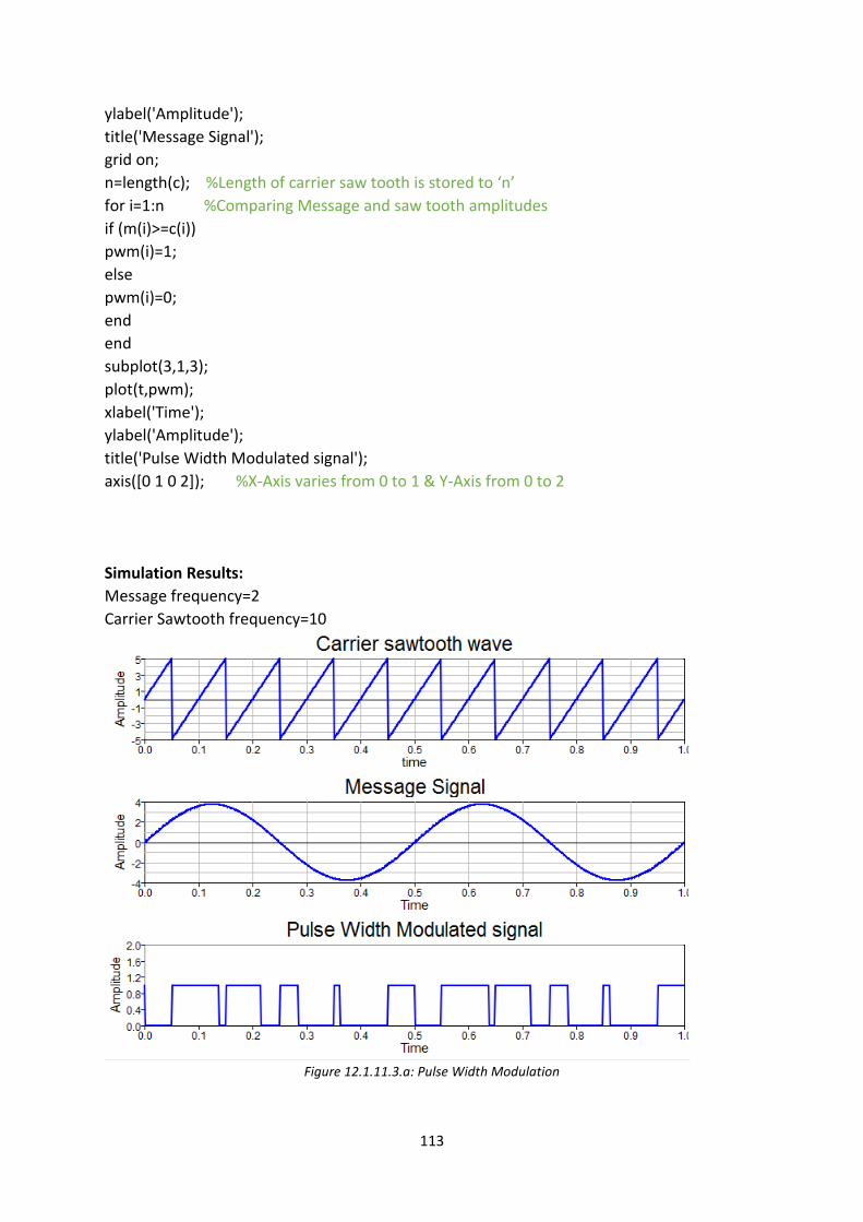
113


title('Message Signal');

grid on;

n=length(c); %Length of carrier saw tooth is stored to ‘n’

for i=1:n %Comparing Message and saw tooth amplitudes

if (m(i)>=c(i))

pwm(i)=1;

else

pwm(i)=0;

end

end

subplot(3,1,3);

plot(t,pwm);

xlabel('Time');


title('Pulse Width Modulated signal');

axis([0 1 0 2]); %X-Axis varies from 0 to 1 & Y-Axis from 0 to 2

Simulation Results:

Message frequency=2

Carrier Sawtooth frequency=10

Figure 12.1.11.3.a: Pulse Width Modulation

114

12.2 STATISTICS

sT Compose has over 85 commands to support statistical processing. A list of general

statistical commands are given below.

mean; median; meandev; pdf; rms; std; rand; randn; var; cdf; corr; cov; erf;

icdf; normcdf; cpsd; detrend; fullfact; geomean; icdf; bbdesign; random; rcond;

regres; skewness; ttest; ttest2; vartest; vartest2; ztest; beta; betacdf; betafit;

betainv; betapdf; betarnd; chi2cdf; chi2inv; chi2pdf; chi2rnd; expcdf; expcurvefit;

exppdf; expfit; expinv; fcdf; fpdf; finv; frnd; gamcdf; gamfit; gaminv; gamma;

gampdf; gamrnd; logncdf; lognfit; logninv; lognpdf; lognrnd; normcdf; normfit;

norminv; normpdf; normrnd; poisscdf; poissfit; poissinv; poisspdf ; poissrnd; tcdf;

tinv; tpdf; trnd; unifcdf; unifffit; unifinv; unifpdf; unifrnd; wblcdf; wblfit; wblinv;

wblpdf; wblrnd; weibcdf; weibfit; weibinv; weibpdf; weibrnd

Example 12.2.1

For the parameter ‘k’, selected as 1,2,3,4,5 draw the Probability density functions and

cumulative distributive functions of 2 distributions.

clc; clear; close;

x=[-eps:-0.02:-0.05, 0:0.02:2];

x=sort(x');

k1=[1 2 3 4 5];y1=[];y2=[];

for i=1:length(k1)

y1=[y1, chi2pdf(x,k1(i))];

y2=[y2, chi2cdf(x,k1(i))];

end

figure(1)

plot(x,y1);grid on;title('probability density function')

figure(2)

plot(x,y2);grid on;title('cumulative distribution function')

115

Simulation results:

Figure 12.2.1.a: PDF’s and CDF’s of 2 distribution

Example 12.2.2

Generate a set of 30000 normally distributed random numbers and find the mean, variance

and standard deviation

%Software Code

p=normrnd(0.5,1.5,30000,1);

[mean(p), var(p), std(p)]

Simulation Results:

ans = [Matrix] 1 x 3 0.48283 2.22144 1.49045

Example 12.2.3

Assume that the linear regression model is y=x1 - 1.232x2+2.23x3 + 2x4 + 4x5 + 3.792 x6.

Calculate the output vector y with 120 measured data points. Also find the undetermined

parameters aint within the given confidence level.

a=[1 -1.232 2.23 2 4 3.792]';

X=randn(120,6);

y=X*a;

[a,a_int,r,ri,stats]=regress(y,X,0.02)

116

Simulation Results:

a = [Matrix] 6 x 1 a_int = [Matrix] 6 x 2

1.00000 1.00000 1.00000

-1.23200 -1.23200 -1.23200

2.23000 2.23000 2.23000

2.00000 2.00000 2.00000

4.00000 4.00000 4.00000

3.79200 3.79200 3.79200

Example 12.2.4

For the parameter, selected as =1,2,5,10. Draw the PDF’s and CDF’s of the poisons

distributions.

clc; clear; close all;

x=[0:15]'; y1=[]; y2=[]; lam1=[1 2 5 10];

for i=1:length(lam1)

y1=[y1, poisspdf(x,lam1(i))];

y2=[y2, poisscdf(x,lam1(i))];

end

figure(1)

plot(x,y1);grid on;

figure(2)

plot(x,y2);grid on;

Simulation Results:

Figure 12.2.4.a: Probability density function and Cumulative distribution function using poisons distribution

117

A set of commands for solving ordinary differential equations are included in sT Compose.

They are

Ode113; ode15i; ode15s; odeset

12.2 5 solving mass spring damper system in sT Compose.

Mass spring damper system is given by the following equation.

0

kxxbxm

Where ‘m’ is the mass, ‘b’ is the damping constant and ‘k’ is the spring constant.

clc; clear;

function dy = md_fun(t,y,b,m,k)

dy = [0, 0]; % State equation

dy(1) = y(2); % State equation

dy(2) = -y(1)*(k/m) - y(2)*(b/m); % State equation

end

m=5; % Mass (kg)

k=2; %Spring Constant

b=1; %Damping Constant

handle = @(t,y) md_fun(t,y,b,m,k);

t = [0:0.2:50]; % Simulation time

yi = [10, 0]; % Initial Condition

[t,y] = ode113(handle,t,yi); % Solving differential equation using solver

i = y(:,1)' % First column values

subplot(1,2,1)

plot(t,i);grid on;

xlabel('time');

ylabel('displacement of the spring');

j=y(:,2)'; % second column values

subplot(1,2,2)

118

plot(t,j); grid on;

xlabel('time');

ylabel('velocity of the spring');

Simulation results:

Figure 12.2.5.a: displacement and velocity of mass damper system wrt time

12.2.6 Solving van Der Pol oscillator system in sT Compose.

The van Der Pol oscillator is a non-conservative oscillator with non-linear damping. It evolves

in time according to the second-order differential equation.

0)1( 2

xxxx where x is the position ccordinate which is a function of the time t, and

is a scalar parameter indicating the nonlinearity and the strength of the damping. This

differential equation is solved in sT Compose as given below.

function dy = vander(t,y,mu)

dy = [0, 0]; % State equation

dy(1) = y(2); % State equation

dy(2) = mu * (1.0 - y(1)^2) * y(2) - y(1); % State equation

end

mu = 1.0; % Scalar parameter

handle = @(t,y) vander(t,y,mu);

t = [0:0.2:40]; % time vector

119

yi = [2, 0]; %initial condition

[t,y] = ode15s(handle,t,yi);

x = y(:,1)'

plot(t,x);

Figure 12.2.6.a: Vander Pol Oscillator system

120

12.3 CONTROL SYSTEMS

12.3.1 Step Response of a second order system

Step response is the time behaviour of the outputs of a general system when its inputs change

from zero to one in a very short time.

2010

1)(

3

sssG

Software code:


sys.num = [1]; % Numerator

sys.den = [1 10 20]; % Denominator

sys1=tf(sys.num,sys.den); % Finding transfer function

kp=dcgain(sys.num,sys.den) % gain when frequency is zero(s=0)

ess=1/(1+kp) % Steady state error

w = sqrt (sys.den(3)) % Finding natural frequency

zeta = sys.den(2) / (2*w) % Damping ratio

TD=(1+0.7*zeta)/w % Delay time

TS = 4/ (zeta*w) % Settling time

TP = pi/ (w*sqrt(1-zeta^2)) % Peak Time

TR=(pi-atan((sqrt(1-zeta^2))/zeta))/(w*sqrt(1-zeta^2)) % Rise Time

Percentovershoot= exp(-zeta*pi/ sqrt(1-zeta^2))*100 % Overshoot

subplot(2,2,1)

[z,t]=step(sys1); % Step response

plot(t,z);

title('Step response');



subplot(2,2,2)

pzmap(sys.num,sys.den); % Pole zero plot

title('Pole zero map of the given system')

grid on;

https://en.wikipedia.org/wiki/System

121

%% Adding Zero to the given system

sys.num = conv(sys.num,[1 1]);

sys2=tf(sys.num,sys.den)

[f,t]=step(sys2);

subplot(2,2,3)

plot(t,f);

title('Step response after addition of zero')



subplot(2,2,4)

pzmap(sys.num,sys.den) % Pole zero plot when zero is added

title('Pole zero map when zero is added')

grid on;

Simulation Results:

sys1 = 1 --------------

1s^2+10s+20

sys2 = 1s+1 ------------- 1s^2+10s+20

kp = 0.05 ( DC gain) ess = 0.952380952 ( Steady state error) w = 4.47213595 (Natural frequency) zeta = 1.11803399 (Damping ratio) TD = 0.398606798 (Delay time) TS = 0.8 (Settling Time) TP = 0 - 1.40496295i (Peak Time) TR = -0.21520447 - 1.40496295i (Rise Time) Percent overshoot = 73.7368878 + 67.5490294i (Percent Overshoot)

122

Figure 12.3.1.a: Step Response and addition of zero to the given system

The following functions are created for finding transfer function, step response, pole zero

map, to find state space matrices and dc gain of the system.

Function created to find the pole zero map of the system

function pzmap(varargin)

if length(varargin)==1

sys=varargin{1}; % assigning structure to variable ‘sys’

num=sys.num; %Numerator

den=sys.den; % Denominator

end

if length(varargin)==2

num=varargin{1}; % Numerator

den=varargin{2}; % Denominator

end

z=roots(num); % Finding zeros

p=roots(den); % Finding poles

%%% …………….For Plotting poles

for i=1:length(p)

R=isreal(p(i)); % Check whether the poles are real or not

123

switch (R)

case 1 % case when Poles are real

p1=[p(i),0]; % Defining first point for plotting poles

p2=[p(i),0]; % Defining second point for plotting poles

theta = atan2( p2(2) - p1(2), p2(1) - p1(1)); % Finding slope

r = sqrt( (p2(1) - p1(1))^2 + (p2(2) - p1(2))^2); % Finding the length between the first and

second point

line = 0:0.01: r;

x = p1(1) + line*cos(theta); % set of x coordinates to plot

y = p1(2) + line*sin(theta); % set of y coordinates to plot

plot(x,y,'x'); % Plotting poles

hold on;

case 0 % Case when poles are imaginary.

p1=[real(p(i)),imag(p(i))];

p2=[real(p(i)),imag(p(i))]; % Since both points(p1 &p2) are equal, it plots only the

specified point

theta = atan2( p2(2) - p1(2), p2(1) - p1(1));

r = sqrt( (p2(1) - p1(1))^2 + (p2(2) - p1(2))^2);

line = 0:0.01: r;

x = p1(1) + line*cos(theta);

y = p1(2) + line*sin(theta);

plot(x,y,'x');

hold on;

end

end

%%%%-----------------For Plotting Zeros

for i=1:length(z)

S=isreal(z(i)) % Check whether the zeros are real or not

switch (S)

case 1 % case when Poles are real

124

q1=[z(i),0];

q2=[z(i),0];

theta = atan2( q2(2) - q1(2), q2(1) - q1(1));

r = sqrt( (q2(1) - q1(1))^2 + (q2(2) - q1(2))^2);

line = 0:0.01: r;

a = q1(1) + line*cos(theta);

b = q1(2) + line*sin(theta);

plot(a,b,'o');

hold on;

case 0 % Case when zeros are imaginary.

q1=[real(z(i)),imag(z(i))];

q2=[real(z(i)),imag(z(i))];

theta = atan2( q2(2) - q1(2), q2(1) - q1(1));

r = sqrt( (q2(1) - q1(1))^2 + (q2(2) - q1(2))^2);

line = 0:0.01: r;

a = q1(1) + line*cos(theta);

b = q1(2) + line*sin(theta);

plot(a,b,'o'); % plotting zeros

hold on;

end

end; end

125

12.3.2 EFFECT OF P, PI, PD, AND PID CONTROLLERS

A controller is a device, historically using mechanical, hydraulic, pneumatic or electronic

techniques often in combination, but more recently in the form of a microprocessor or

computer, which monitors and physically alters the operating conditions of a given

dynamical system.

415.0

1)(

3

sssG

Software Code:


sys.num=[1]; % Numerator of the system is defined as a structure

sys.den=[0.5 1 4]; % Denominator of the system is defined as a structure

sys1=tf(sys) % Print transfer function and store it in sys1.

sys5.num=[1];

sys5.den=[1];

[f,G]=feedback(sys,sys5) % Gives transfer function of the system with unity feedback

[z,t]=step(G); % Step response of the system

subplot(2,3,1);plot(t,z);grid on;

title('Step response of given system');

Figure 12.3.2.a: Step Response of the given system

126

%Proportional controller

kp=10;

sys.num=kp*sys.num; % Numerator augmented with P controller

sys2=tf(sys);

sys6.num=[1];

sys6.den=[1];

[f,G]=feedback(sys,sys6)

[z,t]=step(G);

subplot(2,3,2);

plot(t,z);grid on;

title('Proportional contol Kp=10')

k=dcgain(sys) % DC gain of the system ( s=0)

essP=1/(1+k)

Figure 12.3.2.b: Step Response with P controller

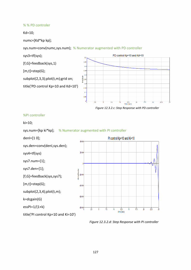
127

% % PD controler

Kd=10;

numc=[Kd*kp kp];

sys.num=conv(numc,sys.num); % Numerator augmented with PD controller

sys3=tf(sys);

[f,G]=feedback(sys,1)

[m,t]=step(G);

subplot(2,3,3);plot(t,m);grid on;

title('PD control Kp=10 and Kd=10')

Figure 12.3.2.c: Step Response with PD controller

%PI controller

ki=10;

sys.num=[kp ki*kp]; % Numerator augmented with PI controller

denI=[1 0];

sys.den=conv(denI,sys.den);

sys4=tf(sys)

sys7.num=[1];

sys7.den=[1];

[f,G]=feedback(sys,sys7);

[m,t]=step(G);

subplot(2,3,4);plot(t,m);

k=dcgain(G)

essPI=1/(1+k)

title('PI control Kp=10 and Ki=10')

Figure 12.3.2.d: Step Response with PI controller

128

% %PID controller

sys.num=conv(numc,[1 ki]); % Numerator augmented with PID controller

sys3=tf(sys);

[f,G]=feedback(sys,1);

[m,t]=step(G);

subplot(2,3,5);plot(t,m);

k=dcgain(G)

essPID=1/(1+k)

title('PID control Kp=10,Ki=10 & kd=10')

Figure 12.3.2.e: Step Response with PID controller

Function defined for feedback command

function [f,G]=feedback(sys1,sys2)

num1=sys1.num; %Numerator of the first system

den1=sys1.den; %Denominator of the first system

num2=sys2.num; %Numerator of the second system

den2=sys2.den; %Denominator of the second system

[num1,den2]=equal_length(num1,den2); % to make numerator and denominator equal

length

[den1,den2]=equal_length(den1,den2);

[num1,num2]=equal_length(num1,num2);

num_n=conv([num1],[den2]); %Numerator of the feedback system

d1=conv([den1],[den2]);

d2=conv([num1],[num2]);

[d1 d2]=equal_length(d1,d2);

den_n=d1+d2; % denominator of the feedback system

G.num=num_n;

G.den=den_n;

f=tf(G);

s1=find(G.num);

s2=find(G.den);

if s1(1)>1

G.num=[G.num(s1(1):length(G.num))]; % to avoid initial unwanted zeros in the numerator

end

if s2(1)>1

G.den=[G.den(s2(1):length(G.den))]; % to avoid initial unwanted zeros in the denominator

129

end

end

Function defined to make numerator and denominator equal length

function [num1,den1]=equal_length(num1,den1)

g=abs(length(den1)-length(num1)); %Difference in the length of numerator and

denominator

% To make numerator equal length with denominator

if length(den1)>length(num1)

for i=length(num1):-1:1

num1(i+g)=num1(i);

end

for l=1:g

num1(l)=0;

end

end

% To make denominator equal length with numerator

if length(num1)>length(den1)

for i=length(den1):-1:1

den1(i+g)=den1(i);

end

for l=1:g

den1(l)=0;

end

end

num1;

den1;

end

130

12.3.3 BODE PLOT AND NYQUIST PLOT

Bode plot is a graph of the frequency response of a system. It is usually a combination

of a Bode magnitude plot, expressing the magnitude (usually in decibels) of the frequency

response, and a Bode phase plot, expressing the phase shift. Both quantities are plotted

against a horizontal axis proportional to the logarithm of frequency

Nyquist plot is a representation of the vector response of a feedback system (especially an amplifier) as a complex graphical plot showing the relationship between feedback and gain.

065

1)(

23

ssssG

% Bode Plot

sys.num=[0 0 0 1]; % Numerator of the system

sys.den=[1 5 6 0]; % denominator of the system

w=logspace(-2,2,100); % Define frequency

magnitude=1./(w.*sqrt(w.^2+3^2).*sqrt(w.^2+2^2)); % Magnitude expression of the given

system

mag_db=20*log10(magnitude); % Magnitude in dB

phase_rad=-atan(w/0)-atan(w/3)-atan(w/2); %Phase angle

phase_deg=phase_rad*180/pi; %Phase angle in degree

figure(2)

subplot(2,1,1)

semilogx(w,mag_db) % Magnitude plot in semilog graph

xlabel('frequency [rad/s]'),ylabel('Magnitude [db]'),grid on;

subplot(2,1,2)

semilogx(w,phase_deg) % Phase plot

xlabel('frequency [rad/s]'),ylabel('Phase Angle [deg]'),grid on;

%%--------Gain Margin

[wgc,fval] = fsolve(@func,5) % gain crossover frequency

gm=1./(wgc.*sqrt(wgc.^2+3^2).*sqrt(wgc.^2+2^2)) % Gain Margin

%--------Phase margin

j=1;

for i=1:length(mag_db)

https://en.wikipedia.org/wiki/Plot_(graphics)

https://en.wikipedia.org/wiki/Frequency_response

https://en.wikipedia.org/wiki/Decibel

https://en.wikipedia.org/wiki/Phase_(waves)

https://en.wikipedia.org/wiki/Logarithm

131

if mag_db(i)>-0.2 && mag_db(i)<0.2 % setting a limit for finding wpm

b(j)=(i);

j=j+1;

end

end

wpm=min(w(b)) % phase crossover frequency

pm=(-atan(wpm/0)-atan(wpm/3)-atan(wpm/2))*180/pi+180 % Phase margin

%---------Function defined for solving gain crossover frequency

function w= func(w)

f=-atan(w/0)-atan(w/3)-atan(w/2)+180;

end

Simulation Results:

Phase crossover frequency, wpm = 0.16297508 Gain margin, gm = Inf Phase margin, pm = 82.23186270

Gain crossover frequency, wgc = 0

Figure 12.3.3.a: Bode plot of the given system

132

Nyquist Plot


sys.num=[0 0 0 1]; % Numerator of the given system

sys.den=[1 5 6 0]; % Denominator of the given system

w=0:-0.01:-10; % Defining frequency for negative values

for i=1:length(w)

real_part(i)=-5*w(i)^2/(25*w(i)^4+(6*w(i)-w(i)^3)^2); % Real part of the given system

end

for i=1:length(w)

imag_part(i)=(w(i)^3-6*w(i))/(25*w(i)^4+(6*w(i)-w(i)^3)^2); % Imaginary part of the given

system

end

plot(real_part,imag_part,'b'); hold on;

axis([-1 0 -2 2]); % Define Axis

fill(real_part(4),1.5, '^'); % To mark the Nyquist plot direction

w=0:0.01:10; % Defining frequency for positive values

for i=1:length(w)

real_part(i)=-5*w(i)^2/(25*w(i)^4+(6*w(i)-w(i)^3)^2);

end

for i=1:length(w)

imag_part(i)=(w(i)^3-6*w(i))/(25*w(i)^4+(6*w(i)-w(i)^3)^2);

end

plot(real_part,imag_part,'b'); hold on;

axis([-1 0 -2 2]); % Define Axis

xlabel('Real Axis'); ylabel('Imaginary Axis');

fill(real_part(4),-1.5, '^');

grid on;

133

Figure 12.3.3.b: Nyquist plot of the given system

134

12.3.4 ROOT LOCUS

To obtain the root locus of the given system whose transfer function is given by

)25.113)(3()(

2

ssss

KsG

Root locus analysis is a graphical method for examining how the roots of a system change with variation of a certain system parameter, commonly a gain within a feedback system.

Software Code:


sys.num=[0 0 0 0 1]

sys.den=[1 6 20.25 33.75 0]

sys1=tf(sys) %Transfer function of the system

rlocus(sys) %Gives Root locus plot

v=[-10,10,-8,8];

axis(v)

xlabel('Real Axis')

ylabel('Imaginary Axis')

title('Root Locus of the system ')

%-------------Function defined for ‘rlocus’

function rlocus(sys)

num=sys.num;

den=sys.den;

%%---------To make numerator and denominator equal length

g=abs(length(den)-length(num));

if length(den)>length(num) % If denominator length is greater than numerator length

for i=length(num):-1:1

num(i+g)=num(i); % shifting numerator coefficients to the right

end

for l=1:g

num(l)=0; % Appending zeros to the index where numerator coefficients originally

existed

135

end

end

if length(num)>length(den) % If numerator length is greater than denominator length

for i=length(den):-1:1

den(i+g)=den(i); % shifting denominator coefficients to the right

end

for l=1:g

den(l)=0; % Appending zeros to the index where denominator coefficients originally

existed

end

end

%%%-------------------------

d=roots(den); % Finding poles

n=roots(num); % Finding zeros

P=length(d); % Number of poles

Z=length(n); % Number of zeros

pzmap(num,den); % P-Z map of the given system

grid on;hold on;

i = 1;

for k=0:0.1:30

r3=den+k*num; % Denominator of unity feedback system for various gain values

r2{i}=roots(r3); % poles of the feedback system

i = i+1;

end

if P==4 && Z==0 % Special case for no zeros and 4 poles

for k=0:2:200

r3=den+k*num;

r2{i}=roots(r3);

i = i+1;

end

136

end

z2=cell2mat(r2); % Conversion of cell to matrix

%---------Extraction of values from the matrix

j=1;

for k=1:length(d)

for i=P+k:length(d):numel(z2)

b(j)=z2(i);

j=j+1;

end

%------Plotting the extracted values

for i=1:numel(b)

p1=[real(b(i)),imag(b(i))]; % Define the first point to plot the root locus

p2=[real(b(i)),imag(b(i))]; % Define the second point to plot the root locus

theta = atan2( p2(2) - p1(2), p2(1) - p1(1)); %Define slope

r = sqrt( (p2(1) - p1(1))^2 + (p2(2) - p1(2))^2); % Distance between first and second point

line = 0:0.01: r;

x = p1(1) + line*cos(theta); % set of x coordinates to plot root locus

y = p1(2) + line*sin(theta); % set of y coordinates to plot root locus

if k==1

plot(x,y,'cyan.'); % plotting different branches with different colour

hold on;

end

if k==2

plot(x,y,'g.'); % plotting different branches with different colour

hold on;

end

if k==3

plot(x,y,'r.'); % plotting different branches with different colour

hold on;

137

end

if k==4

plot(x,y,'b.'); % plotting different branches with different colour

hold on;

end

end

j=1;

end;

Simulation Results:

Figure 12.3.4.a: Root Locus of the system

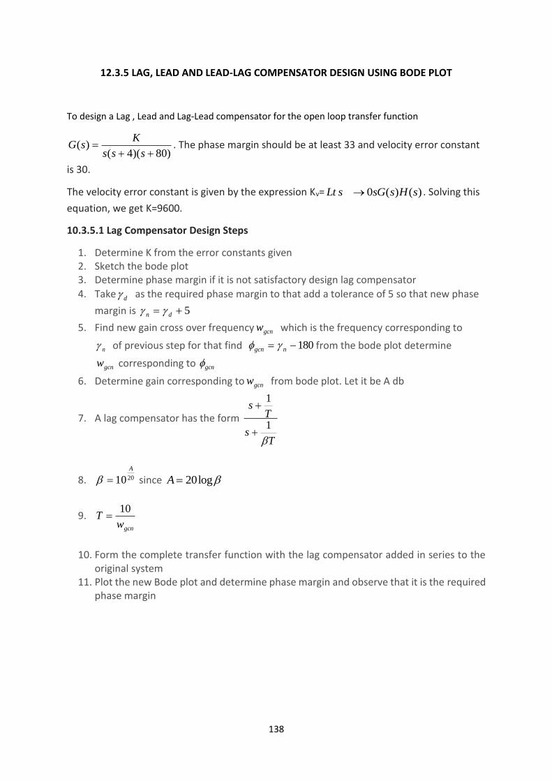
138

12.3.5 LAG, LEAD AND LEAD-LAG COMPENSATOR DESIGN USING BODE PLOT

To design a Lag , Lead and Lag-Lead compensator for the open loop transfer function

)80)(4()(

sss

KsG . The phase margin should be at least 33 and velocity error constant

is 30.

The velocity error constant is given by the expression Kv= )()(0 sHssGsLt . Solving this

equation, we get K=9600.

10.3.5.1 Lag Compensator Design Steps

1. Determine K from the error constants given 2. Sketch the bode plot 3. Determine phase margin if it is not satisfactory design lag compensator

4. Take d as the required phase margin to that add a tolerance of 5 so that new phase

margin is 5 dn

5. Find new gain cross over frequency gcnw which is the frequency corresponding to

n of previous step for that find 180 ngcn from the bode plot determine

gcnw corresponding to gcn

6. Determine gain corresponding to gcnw from bode plot. Let it be A db

7. A lag compensator has the form

Ts

Ts

1

1

8. 2010

A

since log20A

9. gcnw

T10

10. Form the complete transfer function with the lag compensator added in series to the

original system 11. Plot the new Bode plot and determine phase margin and observe that it is the required

phase margin

139

Software code for Lag compensator


K=9600

d1=conv([1 4 0],[1 80]) % Denominator of the given system

G=tf(K,d1) % Transfer function of the given system

%%%-----------Uncompensated system

w=logspace(-2,4,1000); %%frequency range

for k=1:length(w)

mag(k)=9600/(w(k)*sqrt(w(k)^2+4^2)*sqrt(w(k)^2+80^2)); %Magnitude Expression

end

mag_db=20*log10(mag); %Magnitude in dB

phase_rad=-atan(w/0)-atan(w/4)-atan(w/80); %phase in radians

phase_deg=phase_rad*180/pi; %phase in degrees

subplot(2,1,1)

semilogx(w,mag_db) %semi log plot

xlabel('Frequency [rad/s]'),ylabel('Magnitude in db'),grid on %x-axis label

subplot(2,1,2)

semilogx(w,phase_deg)

xlabel('Frequency [rad/s]'),ylabel('Phase Angle [deg]'),grid on

%--------Gain Margin

[wpc,fval] = fsolve(@gain_margin1,5)

gm=9600/(wpc*sqrt(wpc^2+4^2)*sqrt(wpc^2+80^2));

gm=1/gm %Gain Margin

j=1;


if mag_db(i)>-0.2 && mag_db(i)<0.2

b(j)=(i);

j=j+1;

end

140

end

wgc=min(w(b))

pm=(180/pi)*(-atan(wgc/0)-atan(wgc/4)-atan(wgc/80))+180 %Phase Margin of the

uncompensated system

%%%---------------Compensated System

pmreq=input('Enter Required Phase Margin') % enter 33 as given in question

pmreq=pmreq+5

phgcm=pmreq-180

wgcm=4.57784054 % Index is 444. % from the first bode plot, locate wgcm corresponding to

phgcm.

Beta=4.30491478; %Magnitude at wgcm

p=-2.48061788; %Phase at wgcm

T=10/wgcm

Zc=1/T

Pc=1/(Beta*T)

Gc=tf([1 Zc],[1 Pc]) %Compensated System

%%Compensated system= Gc*G/Beta

sys.num=[9600 4394.7264]; %Compensated system numerator

sys.den=[4.3 361.657 1414.41 146.323 0]; %Compensated system denominator

w1=logspace(-2,4,1000); %%frequency range

for k=1:length(w1)

mag(k)=2232.5581*(sqrt(w1(k)^2+0.457784^2))/(w1(k)*sqrt(w1(k)^2+79.99^2)*sqrt(w1(k)^

2+4^2)*sqrt(w1(k)^2+0.10634^2));

end

mag_db=20*log10(mag); %transfer function converted to dB

phase_rad=atan(w/0.457784)-atan(w/0)-atan(w/79.999)-atan(w/4)-atan(w/0.10634);

%phase in radians


figure(2)

subplot(2,1,1)


141

xlabel('Frequency [rad/s]'),ylabel('Magnitude in db'),grid on %x-axis label

subplot(2,1,2)




[wpc1,fval] = fsolve(@gain_margin2,5)

gm1=2232.5581*(sqrt(wpc1^2+0.457784^2))/(wpc1*sqrt(wpc1^2+79.99^2)*sqrt(wpc1^2+4

^2)*sqrt(wpc1^2+0.10634^2));

gm1=1/gm1 Gain Margin of the compensated system

j=1;



b1(j)=(i);

j=j+1;

end

end

wgc1=min(w(b1))

pm1=(180/pi)*(atan(wgc1/0.457784)-atan(wgc1/0)-atan(wgc1/79.999)-atan(wgc1/4)-

atan(wgc1/0.10634))+180 %Phase Margin of the compensated system

Function defined for finding phase crossover frequency of the compensated system

function f= gain_margin2(w1)

f=atan(w1/0.457784)-atan(w1/0)-atan(w1/80)-atan(w1/4)-atan(w1/0.10634)+pi; end;

Function defined for finding phase crossover frequency of the uncompensated system

function f= gain_margin1(w)

f=-atan(w/0)-atan(w/4)-atan(w/80)+pi;

end

142

Simulation Results:

Uncompensated system

Phase Crossover frequency, wpc = 17.8876351 Gain Margin, gm = 2.79971554 Gain Crossover frequency, wgc = 10.4959323 Phase Margin, pm = 13.3873783

Compensated system

Phase crossover frequency, wpc1 = 17.01 Gain Margin, gm1 = 10.926 Gain Crossover frequency, wgc1 = 4.57784054 Phase Margin, pm1 = 33.491133

Figure 12.3.5.1.a: Bode Plot of the uncompensated system

143

Figure 12.3.5.1.b: Bode Plot of the Lag compensated system

10.3.5.2 Lead Compensator Design Steps

1. Determine K from the error constants given 2. Sketch the bode plot 3. Determine phase margin

4. The amount of phase angle to be contributed by lead network is dm ,

where d is the required phase margin and is 5 initially. if the angle is greater than

60then we have to design the compensator as 2 cascade compensator with lead angle

as2

m

5. calculate m

m

sin1

sin1

from bode plot find mw such that it is the frequency

corresponding to the gain /1log(20

6. calculate mw

T1

7. A lead compensator has the form

Ts

Ts

1

1

8. Form the complete transfer function with the lead compensator added in series to th

original system

144

9. Plot the new Bode plot and determine phase margin and observe that it is the required phase margin

10. If not satisfactory repeat steps from step 4 by changing value of by 5

Software code for Lead Compensator

Pd=input('Enter Desired Phase margin')

ep=input('Enter value e') % enter the value of epsilon initially start with 5

ph=Pd-pm+ep

if ph>60 % check if angle needed is greater than 60

phm=ph/2

else

phm=ph

end

alpha=(1-sind(phm))/(1+sind(phm)) % calculate alpha

db=-20*log10(1/sqrt(alpha)) %calculate the gain in db

wm=13.462 % from plot obtain frequency corresponding to above gain

T=1/(wm*sqrt(alpha))

Gc=tf([1 1/T],[1 1/(alpha*T)]) % form transfer function of compensator

if ph==phm

%%Go=Gc*G/alpha is the transfer fn of the compensated system

Go.num=[37944.664 258023.715]; %Compensated system Numerator

Go.den=[1 110.8 2571.2 8576 0]; %Compensated system Denominator

%Go=Gc*Gc*G %‘Cascade’

%If angle was greater than 60 we designed compensator for half value so we cascade them

and their attenuation is not nullified and should be retained

end

w1=logspace(-2,4,1000); %%frequency range

for k=1:length(w1)

mag(k)=37944.664*(sqrt(w1(k)^2+6.8^2))/(w1(k)*sqrt(w1(k)^2+80^2)*sqrt(w1(k)^2+4^2)*s

qrt(w1(k)^2+26.8^2));

end

145

mag_db=20*log10(mag); %transfer function magnitude converted to dB

phase_rad=atan(w/6.8)-atan(w/0)-atan(w/80)-atan(w/4)-atan(w/26.8); %phase in radians


figure(2)

subplot(2,1,1)


xlabel('Frequency [rad/s]'),ylabel('Magnitude in db'),grid on %xaxis label

subplot(2,1,2)




[wpc1,fval] = fsolve(@gain_margin3,5)

gm1=37944.664*(sqrt(wpc1^2+6.8^2))/(wpc1*sqrt(wpc1^2+80^2)*sqrt(wpc1^2+4^2)*sqrt(

wpc1^2+26.8^2));

gm1=1/gm1 %Gain Margin of the compensated system

j=1;



b1(j)=(i);

j=j+1;

end

end

wgc1=min(w(b1))

pm1=(180/pi)*(atan(wgc1/6.8)-atan(wgc1/0)-atan(wgc1/80)-atan(wgc1/4)-

atan(wgc1/26.8))+180 %Phase Margin of the compensated system

[f,comp]=feedback(Go,1); %Gives transfer function with unity feedback

[f1, uncomp]=feedback(G,1);

[z,t]=step(uncomp); % observe step response

figure(3)

plot(t,z,'b');

146

hold on

[z1,t]=step(comp); %Step Response of the compensated system

plot(t,z1,'r');

grid on;

legend('Uncompensated’, ‘Compensated')



f=atan(w/6.8)-atan(w/0)-atan(w/80)-atan(w/4)-atan(w/26.8)+pi;

end

Simulation Results:

Desired Phase margin given= 45; ep=5;

Phase Crossover frequency, wpc1 = 43.0032803 Gain Margin, gm1 = 5.17396972 Gain Crossover Frequency, wgc1 = 15.6745541 Phase Margin, pm1 = 39.4556603

Figure 12.3.5.2.a: Bode Plot of the Lead compensated system

147

Figure 12.3.5.2.b: Step response of the compensated system and uncompensated system

10.3.5.3 LEAD-LAG COMPENSATOR DESIGN

Design Steps:

1. For the specified error constant, find the open loop gain K.

2. Draw the magnitude and phase spectrum of the uncompensated system with this K

and determine the phase margin and gain crossover frequency.

3. Design the lag section to provide only the partial compensation of phase margin.

Choose the gain crossover frequency such that it is higher than the gain crossover

frequency if the system was fully compensated.

4. Determine the value of required such that the high frequency attenuation

provided by the lag network is equal to the magnitude of the uncompensated system

at this frequency.

5. Calculate the value of 1 such that the upper cut-off frequency of the lag network is

two octaves below the gain crossover frequency.

6. Calculate the lower cut-off frequency

11 /1 .

Find its transfer function and draw the magnitude and phase plot of the lag

compensated system and determine gain crossover frequency and the phase margin.

148

7. For the lead section design, independent value of cannot be chosen. So select

1 and calculate the maximum phase-lead provided by the lead section using

the formula

1

1sin 1

m =

/11

/11sin 1

8. To fully utilize the lead effect, choose the compensated crossover frequency to

coincide with 2/1m . So calculate 2 and 2 and write the lead

compensator transfer function.

9. Combine the transfer functions of lag and lead sections to get the lead lag

compensator transfer function. Draw the bode plot and determine the phase

margin.

Software Code for Lead Lag Compensator

clc; close all; clear all % clear all variables

K=9600 % value of K calculated from error constants

G.num=K;

G.den=conv([1 4 0],[1 80]); %Given System

w=logspace(-2,4,1000);

%%%---------Lead Lag Compensator

%Lag Compensator TF

sys1.num=[1 0.457784];

sys1.den=[1 0.10634];

%Lead Compensator TF

sys2.num=[1 6.76882];

sys2.den=[1 26.7736];

%Lead Lag Compensator TF

sys3.num=[9600 69375.3984 29747.11195];

z1=conv([sys1.den],[sys2.den]);

z2=conv([1 4],[1 80]);

z3=conv([1],[z2]);

sys3.den=conv([z3],[z1])

for k=1:length(w)

149

mag(k)=9600*(sqrt(w(k)^2+0.457784^2)*sqrt(w(k)^2+6.76822^2))/(w(k)*sqrt(w(k)^2+4^2)*

sqrt(w(k)^2+80^2)*sqrt(w(k)^2+0.10634^2)*sqrt(w(k)^2+26.7746^2));

end

mag_db=20*log10(mag); %transfer function converted to dB

phase_rad=atan(9600*w/4394.7264)+atan(w/6.76882)-atan(w/0)-atan(w/4)-atan(w/80)-

atan(w/0.10634)-atan(w/26.7736); %phase done in radians

phase_deg=phase_rad*180/pi; %phase done in degrees

subplot(2,1,1)


xlabel('Frequency [rad/s]'),ylabel('Magnitude in db'),grid on %xaxis label

subplot(2,1,2)




[wpc,fval] = fsolve(@gain_margin4,5)

gm=9600*(sqrt(wpc^2+0.457784^2)*sqrt(wpc^2+6.76822^2))/(wpc*sqrt(wpc^2+4^2)*sqrt(

wpc^2+80^2)*sqrt(wpc^2+0.10634^2)*sqrt(wpc^2+26.7746^2));

gm=1/gm

%--------Phase Margin

j=1;



b(j)=(i);

j=j+1;

end

end

wgc=min(w(b))

pm=(180/pi)*(atan(9600*wgc/4394.7264)+atan(wgc/6.76882)-atan(wgc/0)-atan(wgc/4)-

atan(wgc/80)-atan(wgc/0.10634)-atan(wgc/26.7736))+180

sys4.num=1;

sys4.den=1;

150

[f,comp]=feedback(sys3,sys4);

[f1, uncomp]=feedback(G,sys4);

[z,t]=step(uncomp); % observe step response

figure(3)

plot(t,z,'b');

hold on

[z1,t]=step(comp);

plot(t,z1,'r');

grid on;

legend('Uncompensated','Compensated')



f=atan(9600*w/4394.7264)+atan(w/6.76882)-atan(w/0)-atan(w/4)-atan(w/80)-

atan(w/0.10634)-atan(w/26.7736)+pi;

end

Simulation Results:

Figure 12.3.5.3.a: Bode Plot of the lead-lag compensated system

151

Figure 12.3.5.1.a: Step Response of the uncompensated and lead-lag compensated system

152

12.3.6 REAL TIME CONTROL OF INVERTED PENDULUM

Figure 12.3.6.a: Inverted Pendulum

We will consider a two-dimensional problem where the pendulum is constrained to

move in the vertical plane shown in the figure below. The inverted pendulum system is an

example commonly found in control system textbooks and research literature. Its popularity

derives in part from the fact that it is unstable without control, that is, the pendulum will

simply fall over if the cart isn't moved to balance it. Additionally, the dynamics of the system

are nonlinear. The objective of the control system is to balance the inverted pendulum by

applying a force to the cart that the pendulum is attached to. A real-world example that

relates directly to this inverted pendulum system is the attitude control of a booster rocket

at take-off. For this system, the control input is the force that moves the cart horizontally

and the outputs are the angular position of the pendulum and the horizontal position of the

cart .

The transfer function with the cart position X(s) as the output can be derived as

sq

bmgls

q

mglmMs

qmlIb

s

q

gmlsmlI

sU

sXsPcart

23

24

22

)()(

)(

)(

)()(

Software Code: clc; clear all; close all; M = 0.5; %Mass of the cart m = 0.2; %Mass of the pendulum b = 0.1; %Coefficient of friction of cart I = 0.006; %Mass moment of inertia of the pendulum g = 9.8; %Acceleration due to gravity l = 0.3; %length to pendulum centre of mass q = (M+m)*(I+m*l^2)-(m*l)^2; sys.num=[m*l/q 0]; sys.den=[1 b*(I+m*l^2)/q -(M+m)*m*g*l/q -b*m*g*l/q]; tf_pend=tf(sys) [y1,t]=impulse(sys) figure(1)

153

plot(t,y1); Kp = 100; Ki = 1; Kd = 20; pids.num=[20 100 1]; pids.den=[1 0]; pid=tf(pids) [T,G] = feedback(sys,pids); [y,t]=impulse(G) figure(2) plot(t,y); axis([0, 2.5, 0, 0.05]); Function created for finding Impulse Response function[y,t]=impulse(sys) b=sys.num; a=sys.den; [A,B,C,D]=tf2ss(b,a); t=0:0.01:10; f=length(A); for i=1:length(t) h{i}=(C*(e^(A*t(i)))*(0+B))+D*1*1; end y=cell2mat(h); end Simulation Results:

Figure 12.3.6.b: Impulse Response of the system

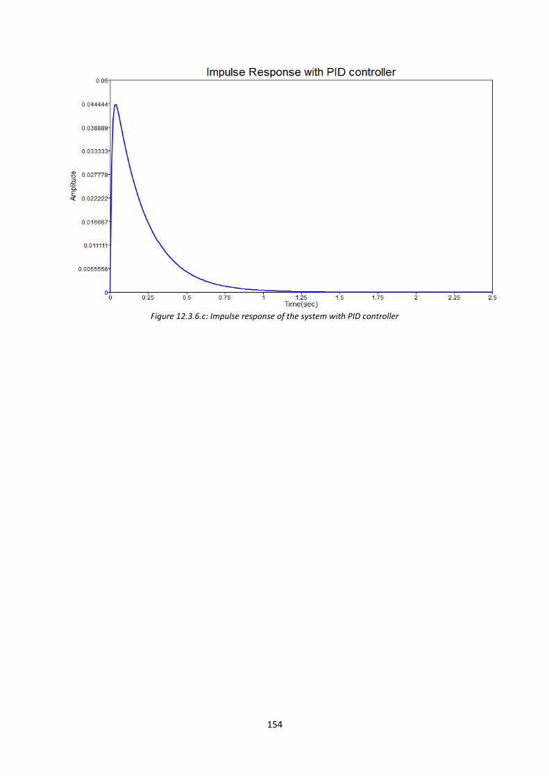
154

Figure 12.3.6.c: Impulse response of the system with PID controller

155

12.4 Optimization and Solving

This section introduces you about optimisation and solving using nonlinear programming and

genetic algorithm. This tutorial demonstrates each solver by finding the minimum distance

between two non-intersecting ellipsoids defined as follows:

19

)3(

16

)2(

25

)1( 222

zyx

136

)14(

81

)13(

49

)12( 222

zyx

12.4.1 Non Linear Programming

SOLVING USING ‘fsolve’

function res = Residuals(v)

% define v = [x1, y1, z1, x2, y2, z2, lambda1, lambda2], where lambda1, lambda2 are

Lagrange Multipliers

f_grad = 2*[v(1)-v(4), v(2)-v(5), v(3)-v(6), v(4)-v(1), v(5)-v(2), v(6)-v(3)];

g1_grad = 2*[(v(1)-1)/25, (v(2)-2)/16, (v(3)-3)/9, 0, 0, 0];

g2_grad = 2*[0, 0, 0, (v(4)-12)/49, (v(5)-13)/81, (v(6)-14)/36];

res = zeros(8,1);

res(1:6) = f_grad - v(7) * g1_grad - v(8) * g2_grad;

res(7) = (v(1)-1)^2/25 + (v(2)-2)^2/16 + (v(3)-3)^2/9 - 1;

res(8) = (v(4)-12)^2/49 + (v(5)-13)^2/81 + (v(6)-14)^2/36 - 1;

end

v0 = [1.1,2.2,3.3,17.2,18.3,19.4,-1,1]; % initial estimate of v

[v,fval] = fsolve(@Residuals, v0);

p1 = v(1:3)

p2 = v(4:6)

d = norm(p1-p2)

Simulation Results:

p1 = [Matrix] 1 x 3 4.35329 3.94398 4.68114

156

p2 = [Matrix] 1 x 3 8.40015 7.60969 10.31684 d = 7.84701501 SOLVING USING ‘fmincon’

function [obj] = ObjFunc(v) % define v = [x1, y1, z1, x2, y2, z2] obj = (v(1)-v(4))^2 + (v(2)-v(5))^2 + (v(3)-v(6))^2; end % Nonlinear constraint functions function [c, ceq] = ConFunc(v) % inequality c = []; % equality ceq = [0; 0]; ceq(1) = (v(1)-1)^2/25 + (v(2)-2)^2/16 + (v(3)-3)^2/9 - 1; ceq(2) = (v(4)-12)^2/49 + (v(5)-13)^2/81 + (v(6)-14)^2/36 - 1; end v0 = [1.1,2.2,3.3,12.2,13.3,14.4]; % initial estimate of v lowerBound = [0, 0, 0, 0, 0, 0]; upperBound = [20, 20, 20, 20, 20, 20]; [v,fval] = fmincon(@ObjFunc,v0,[],[],[],[],lowerBound,upperBound,@ConFunc); p1 = v(1:3) p2 = v(4:6) d = norm(p1-p2) Simulation Results:

p1 = [Matrix] 1 x 3 4.35326 3.94394 4.68119 p2 = [Matrix] 1 x 3 8.40024 7.60967 10.31680 d = 7.84701504 SOLVING USING ‘fmincon’

function obj = ObjFunc(v) % define v = [x1, y1, z1, x2, y2, z2] obj = (v(1)-v(4))^2 + (v(2)-v(5))^2 + (v(3)-v(6))^2; end % Nonlinear constraint functions function c = ConFunc(v)

157

% we can use inequality constraints because we know the solution is on the boundary. % this ga demo works better this way than with equality constraints. c = [0; 0]; c(1) = (v(1)-1)^2/25 + (v(2)-2)^2/16 + (v(3)-3)^2/9 - 1; c(2) = (v(4)-12)^2/49 + (v(5)-13)^2/81 + (v(6)-14)^2/36 - 1; end v0 = [3, 3, 3, 11, 11, 11]; % initial estimate of v lowerBound = [0, 0, 0, 0, 0, 0]; upperBound = [20, 20, 20, 20, 20, 20]; options = gaoptimset('InitialPopulation', v0, 'PopulationSize', 200); [v,fval] = ga(@ObjFunc,6,[],[],[],[],lowerBound,upperBound,@ConFunc,options); p1 = v(1:3) p2 = v(4:6) d = norm(p1-p2) Simulation Results:

p1 = [Matrix] 1 x 3 4.35326 3.94394 4.68119 p2 = [Matrix] 1 x 3 8.40024 7.60967 10.31680 d = 7.84701504 12.4.2 Genetic Algorithm

% Genetic Algorithm SOLVING USING ‘ga’

function obj = ObjFunc(v) % define v = [x1, y1, z1, x2, y2, z2] obj = (v(1)-v(4))^2 + (v(2)-v(5))^2 + (v(3)-v(6))^2; end % Nonlinear constraint functions function c = ConFunc(v) % we can use inequality constraints because we know the solution is on the boundary. % this ga demo works better this way than with equality constraints. c = [0; 0]; c(1) = (v(1)-1)^2/25 + (v(2)-2)^2/16 + (v(3)-3)^2/9 - 1; c(2) = (v(4)-12)^2/49 + (v(5)-13)^2/81 + (v(6)-14)^2/36 - 1; end v0 = [3, 3, 3, 11, 11, 11]; % initial estimate of v lowerBound = [0, 0, 0, 0, 0, 0];

158

upperBound = [20, 20, 20, 20, 20, 20]; options = gaoptimset('InitialPopulation', v0, 'PopulationSize', 200); [v,fval] = ga(@ObjFunc,6,[],[],[],[],lowerBound,upperBound,@ConFunc,options); p1 = v(1:3) p2 = v(4:6) d = norm(p1-p2) Simulation Results:

p1 = [Matrix] 1 x 3 4.35326 3.94394 4.68119 p2 = [Matrix] 1 x 3 8.40024 7.60967 10.31680 d = 7.84701504 12.4.3 Nonlinear Equality Constraints Optimization Problem

Reference: J.Guo and C.Han, “Design of Guidance Laws for Lunar Pinpoint Soft Landing ,” in

AAS/AIAA Astrodynamics Specialist Conf., Pittusburgh, Pennsylvania, 2009, pp. 2133-2146.

An interplanetary mission is a trip through outer space from one planetary body to

another. Soft landing on planetary surface implies that the touchdown happens with a

minimum impact on the on-board instruments. A rover may be placed on the surface of the

celestial body for detailed scientific exploration. The below example is focused on the

minimization of Lander orientation which is a critical parameter during the fine braking and

vertical descent phase of the Lunar landing mission.

The linearized Lander dynamics are given by

cFm

rm

Fv

m

Fu

vy

ux

2cos

sin

‘F’ is the landing thrust force and is the attitude angle between the thrust direction and the

radial vector. Here ‘x’ indicates the horizontal distances between the Lander and the landing

site, and y stands for the vertical distance from the lunar centre to the Lander. ‘m’ is the mass

of the Lander and is the gravity constant of the moon. ‘cF’ is the decreasing rate of mass.

The optimization problem explained in this section is applicable for constant thrust engines.

159

The Lander orientation is given by the equation

12 ktk

Where is a constant angle that contributes for soft landing and k1 and k2 are constants.

The linearized model for the equation of motion of the lander are

vy

8721

07621

06521

0

5421

04321

03221

0221

0

1077

21066

21055

210

4421

03321

02221

021010

)sin(5040

)sin(720

)cos(120

)sin(24

)cos(6

)sin(2

)cos(

)sin()cos(5040

)sin(720

)cos(120

)sin(24

)cos(6

)sin(2

)cos()sin(

tkkT

atkk

T

atkk

T

a

tkkT

atkk

T

atkk

T

atkk

T

a

tkT

atkk

atkk

atkk

a

tkka

tkka

tkka

tkkakau

2

87

21076

21065

210

54

21043

21032

2102

210

1077

21066

21055

210

44

21033

21022

210

21010

)sin(5040

)cos(720

)sin(120

)cos(24

)cos(6

)cos(2

)sin(

)cos()sin(5040

)cos(720

)sin(120

)cos(24

)cos(6

)cos(2

)sin()cos(

Rtkk

T

atkk

T

atkk

T

a

tkkT

atkk

T

atkk

T

atkk

T

a

tkT

atkk

atkk

atkk

a

tkka

tkka

tkka

tkkakav

In the above equations, 0m

cFT . )sin( and )cos( are expanded using Taylor series.

Now the optimization problem is given by

)(.min t Subject to the following constraints

0

1800

0

0

..

min

max

min

min

y

x

v

u

ts

160

Step1: Define the objective function

Figure 12.4.3.a: Objective Function

Step 2: Define the function for the equality constraints

Figure 12.4.3.b: Equality Constraints

Step 3: Initialization of Guidance parameters

Figure 12.4.3.c: Guidance Parameters

Step 4: Solve using fmincon constrained optimization routine

The values of variable ‘a’ represents the solutions obtained using fmincon routine.

a(1) represents time, a(2) represents ,a(3) represents 1k and a(4) represents 2k

respectively in the code wrt equations of motion.

161

Step 5: Calculate the Lander parameters

The Lander parameters like Horizontal distance, Altitude, vertical velocity and horizontal

velocity are calculated using the equations of motion from the solution obtained from

fmincon routine. The loop for finding the above mentioned parameters are executed till the

time provided by the fmincon routine is approached.

Figure 12.4.3.d: Equations of Motion

Step 6: Calculate the lander orientation and acceleration

Horizontal and vertical acceleration profiles of the lander are calculated from the

horizontal and vertical velocities. The lander orientation is also found out then from the

acceleration profile.

Figure 12.4.3.e: Lander Orientation and Accelaration equations

162

Step 7: Plot the results

Figure 12.4.3.f: Plotting Section

During the initiation of the fine braking phase, the Lander is assumed to be situated at an

altitude of 4000m from the lunar surface with a vertical velocity of -75m/s and a horizontal

velocity of 100m/s. The Lander has to be touched down on the lunar surface with a minimum

velocity to prevent the on-board engines from damage. The simulation shows that the Lander

has reached the surface with almost zero horizontal and vertical velocity. During the final

time, the Lander has travelled a horizontal distance of 1800m which is the same as that of

mentioned in the constraint equations.

Figure 12.4.3.g: Velocity and Down range

163

The below figure shows the vertical and horizontal acceleration profiles of the Lander. Both

accelerations are coming down to zero which indicates that the Lander is safe to land on the surface.

Figure 12.4.3.h: Acceleration Profile

The Lander orientation is shown in the below figure. Initially the Lander is oriented at -140

degree. At the end of the mission, it can be seen that the orientation is reduced to zero which

means that the Lander orientation is zero and ready to land on the surface.

Figure 12.4.3.i: Lander Orientation

164

12.5 GUI CREATION IN COMPOSE 12.5.1: To obtain Step response with a slider for various damping ratio for the second order system provided by the user Software Code: clc; close all; clear global num1 global den1 figure('units', 'normalized', 'position', [0.25 0.25 0.5 0.5]) axes('units', 'normalized', 'position', [0.2 0.05 0.8 0.8]); txt1 = uicontrol('Style','text','Position',[1 45 130 30],'String','Num coefficients'); txt0 = uicontrol('Style','text','units','normalized', 'Position', [0.02 0.010 0.86 0.04],'String','Response of a second order system for various Damping Ratio'); % %-------Add a edit box to input numerator coefficients txtbox1 = uicontrol('Style','edit','String','Numerator','Position',[1 70 130 25],'callback',@func1); % %------Add a text uicontrol to enter denominator coefficients txt2 = uicontrol('Style','text','Position',[1 100 130 45],'String','Den coefficients'); % %------Add a edit box to input denominator coefficients txtbox2 = uicontrol('Style','edit','String','Denominator','Position',[1 135 130 25],'callback',@func2); txt1 = uicontrol('Style','text','position',[320 460 100 20],'string','Damping Ratio'); txt2 = uicontrol('Style','text','position',[100 460 10 20],'string','0'); txt3 = uicontrol('Style','text','position',[590 460 10 20],'string','1'); btn=uicontrol('Style','toggle','string','Clear Fig.','Position',[1 180 120 25],'callback', @clear_axes); h=uicontrol('Style','slider','min',0,'max',100,'value',75,'position',[100 420 500 30],'callback', @uistepr); function [btn,h]=uistepr(handle, callbackdata) global num1; global den1; zeta=get(handle,'value')/100; time=0:0.002:5; num=num1; %den=[1 10*zeta 25]; x = den1(2)*zeta; den = [den1(1) x den1(3)]; sys = tf(num,den); [values,time]=step(sys,[0:0.1:10]); plot(time,values); title('Step Response') xlabel('Time(sec)'); ylabel('Amplitude'); hold on; grid on;

165

end function func1(handle,callbackdata) global num1 %----To get the numerator a=get(handle,'String'); %----To convert the numerator string to numeric num1 = str2num(a); end function func2(handle,callbackdata) global den1 %----To get the numerator b=get(handle,'string'); %----To convert the denominator string to numeric den1=str2num(b); end function clear_axes(handle,callbackdata) val=get(handle,'value'); if val == 1 cla; end end Simulation Results:

Figure 12.5.1.a: Step Response for various Damping Ration

166

12.5.2: STEP RESPONSE/ BODE PLOT/ ROOT LOCUS USING GUI Software Code: clc; clear; close all; f = figure('units', 'normalized', 'position', [0.25 0.25 0.5 0.5]) axes('units', 'normalized', 'position', [0.2 0.05 0.8 0.8]); %-------Add a text uicontrol to enter the numerator coefficients txt1 = uicontrol('Style','text','Position',[1 45 130 30],'String','Num coefficients'); % %-------Add a edit box to input numerator coefficients txtbox1 = uicontrol('Style','edit','String','Numerator','Position',[1 70 130 25],'callback',@func1); % %------Add a text uicontrol to enter denominator coefficients txt2 = uicontrol('Style','text','Position',[1 100 130 45],'String','Den coefficients'); % %------Add a edit box to input denominator coefficients txtbox2 = uicontrol('Style','edit','String','Denominator','Position',[1 135 130 25],'callback',@func2); % %-----Add a text uicontrol to select the response txt3 = uicontrol('Style','text','Position',[1 220 140 30],'String','Select the response'); % %----Add a popup menu to select the type of response the user wants to obtain pop_up=uicontrol('Style','popup', 'String',{'Select','Bode Plot','Root Locus','step Response'},'position',[1 250 100 20],'callback',@func); global num1 global den1 function func1(handle,callbackdata) global num1 %----To get the numerator a=get(handle,'String'); %----To convert the numerator string to numeric num1 = str2num(a); end function func2(handle,callbackdata) global den1 %----To get the numerator b=get(handle,'string'); %----To convert the denominator string to numeric den1=str2num(b); end function func3(handle,callbackdata) global num1; global den1; value=get(handle,'value'); if (value==1) cla; w=logspace(-2,4,1000); bode(num1,den1,value,w)

167

end if (value==2) cla; w=logspace(-2,4,1000); bode(num1,den1,value,w) end end function func(handle,callbackdata) global num1 global den1 sys.num=num1; sys.den=den1; %---To obtain bode plot value=get(handle,'value') if (value==2) txt1 = uicontrol('Style','text','Position',[1 290 150 20],'String','Select required plot:'); list_utility = uicontrol('Style','listbox','string',{'Magnitude Plot','Phase Plot'},'Position',[1 310 100 50],'Value',1,'callback',@func3); end %----To obtain root locus if (value==3) rlocus(sys) end %-----To obtain step response if (value==4) cla; system1 = tf(num1,den1); [z,t]=step_response(system1); plot(t,z); grid; title('Step Response'); xlabel('Time(sec)'); ylabel('Amplitude'); end end %--User defined function for bode function bode(num,den,value,w) sys.num = num; sys.den = den; P=roots(sys.den) Z=roots(sys.num) %%%%-----------Magnitude if length(Z)==0 magnitude_z=1*sys.num; end

168

if length(Z)~=0 temp_old_z=1; for j=1:length(Z) for i=1:length(w) temp_new_z(i)=sqrt((w(i))^2+(Z(j))^2); end temp_old_z=temp_old_z.*temp_new_z; end for i=1:length(temp_old_z) magnitude_z(i)=temp_old_z(i); end end if length(P)==0 magnitude_p=1*sys.den; end if length(P)~=0 temp_old_p=1; for j=1:length(P) for i=1:length(w) temp_new_p(i)=sqrt((w(i))^2+(P(j))^2); end temp_old_p=temp_old_p.*temp_new_p; end for i=1:length(temp_old_p) magnitude_p(i)=temp_old_p(i); end end if (length(sys.num)==1) z1=1; end if (length(sys.num)==2) z1=gcd(sys.num(1),sys.num(2)); end if (length(sys.num)==3) z1=gcd(sys.num(1),sys.num(2),sys.num(3)); end if (length(sys.num)==4) z1=gcd(sys.num(1),sys.num(2),sys.num(3),sys.num(4)); end if (length(sys.num)==5) z1=gcd(sys.num(1),sys.num(2),sys.num(3),sys.num(4),sys.num(5)); end magnitude=z1*(magnitude_z./magnitude_p); %%%%---------------Phase Angle if length(Z)==0 temp_old_ph_z=0; end

169

if length(Z)~=0 for i=1:length(w) for j=1:length(Z) temp_new_ph_z(j)=atan(-w(i)/Z(j)); end z1=cumsum(temp_new_ph_z); temp_old_ph_z(i)=z1(end); end end if length(P)==0 temp_old_p_ph=0; end if length(P)~=0 for i=1:length(w) for j=1:length(P) if P(j)~=0 temp_new_ph_p(j)=atan(-w(i)/P(j)); end if P(j)==0 temp_new_ph_p(j)=atan(w(i)/P(j)); end end z2=cumsum(temp_new_ph_p); temp_old_ph_p(i)=z2(end); end end phase_rad=temp_old_ph_z-temp_old_ph_p; if value ==1 mag_db=20*log10(magnitude); phase_deg=phase_rad*180/pi; %phase done in degrees semilogx(w,mag_db) %semilog plot xlabel('Frequency [rad/s]'),ylabel('Magnitude[db]'),grid on %xaxis label title('Magnitude Plot') end if value==2 phase_deg=phase_rad*180/pi; %phase done in degrees semilogx(w,phase_deg) xlabel('Frequency [rad/s]'),ylabel('Phase angle [deg]'),grid on end end %---User Defined Function for pzmap function pzmap(varargin) if length(varargin)==1 sys=varargin{1}; num=sys.num;

170

den=sys.den; end if length(varargin)==2 num=varargin{1}; den=varargin{2}; end z=roots(num); p=roots(den); for i=1:length(p) R=isreal(p(i)); switch (R) case 1 p1=[p(i),0]; p2=[p(i),0]; theta = atan2( p2(2) - p1(2), p2(1) - p1(1)); r = sqrt( (p2(1) - p1(1))^2 + (p2(2) - p1(2))^2); line = 0:0.01: r; x = p1(1) + line*cos(theta); y = p1(2) + line*sin(theta); plot(x,y,'x'); hold on; case 0 p1=[real(p(i)),imag(p(i))]; p2=[real(p(i)),imag(p(i))]; theta = atan2( p2(2) - p1(2), p2(1) - p1(1)); r = sqrt( (p2(1) - p1(1))^2 + (p2(2) - p1(2))^2); line = 0:0.01: r; x = p1(1) + line*cos(theta); y = p1(2) + line*sin(theta); plot(x,y,'x'); hold on; end end %%%%-----------------Zeros for i=1:length(z) S=isreal(z(i)); switch (S) case 1 q1=[z(i),0]; q2=[z(i),0]; theta = atan2( q2(2) - q1(2), q2(1) - q1(1)); r = sqrt( (q2(1) - q1(1))^2 + (q2(2) - q1(2))^2); line = 0:0.01: r; a = q1(1) + line*cos(theta); b = q1(2) + line*sin(theta); plot(a,b,'o'); hold on;

171

case 0 q1=[real(z(i)),imag(z(i))]; q2=[real(z(i)),imag(z(i))]; theta = atan2( q2(2) - q1(2), q2(1) - q1(1)); r = sqrt( (q2(1) - q1(1))^2 + (q2(2) - q1(2))^2); line = 0:0.01: r; a = q1(1) + line*cos(theta); b = q1(2) + line*sin(theta); plot(a,b,'o'); hold on; end end end %---User Defined Function for rlocus function rlocus(sys) num=sys.num; den=sys.den; %%---------To make numerator and denominator equal length g=abs(length(den)-length(num)); if length(den)>length(num) for i=length(num):-1:1 num(i+g)=num(i); end for l=1:g num(l)=0; end end if length(num)>length(den) for i=length(den):-1:1 den(i+g)=den(i); end for l=1:g den(l)=0; end end %%%------------------------- d=roots(den); n=roots(num); P=length(d); Z=length(n); pzmap(num,den); grid on;hold on; i = 1; for k=0:0.01:30 r3=den+k*num; r2{i}=roots(r3);

172

i = i+1; end if P==4 && Z==0 for k=0:2:500 r3=den+k*num; r2{i}=roots(r3); i = i+1; end end z2=cell2mat(r2); j=1; for k=1:length(d) for i=P+k:length(d):numel(z2) b(j)=z2(i); j=j+1; end end scatter(real(b),imag(b),'b.'); title('Root Locus'); xlabel('Real Axis'); ylabel('Imaginary Axis'); end Simulation Results: Step Response:

Figure 12.5.2.a: Step Response for the user provided transfer function

173

Root Locus:

Figure 12.5.2.b:Root Locus of the given system

Bode Plot:

Figure 12.5.2.c: Magnitude Plot of the given system

174

Figure 12.5.2.d: Phase Plot of the given system

12.5.3: SIGNAL OPERATIONS USING GUI clc; clear; close all; f = figure('units', 'normalized', 'position', [0.25 0.25 0.5 0.5]) axes('units', 'normalized', 'position', [0.2 0.2 0.8 0.8]); global vector1; global vector2; %----Creates a text for the Ist sequence txt1 = uicontrol('Style','text','Position',[25 5 180 30],'String','Enter I st sequence'); %----Creates an edit box for the Ist sequence to be entered txtbox1 = uicontrol(f,'Style','edit','String','[ ]','Position',[150 5 120 30],'callback',@func9); %----Creates a text for the IInd sequence txt2 = uicontrol('Style','text','Position',[25 40 180 30],'String','Enter II nd sequence'); %----Creates an edit box for the IInd sequence to be entered txtbox2 = uicontrol(f,'Style','edit','String','[ ]','Position',[150 40 120 30],'callback',@func10); %---Creates a text for the operation to be selected txt3 = uicontrol('Style','text','Position',[400 -8 180 30],'String','Select the operation required'); %----Creates toggle buttons for various operations in signal processing btn1=uicontrol('Style','toggle','string','Linear Convolution','Position',[300 20 180 20],'callback',@func1); btn2=uicontrol('Style','toggle','string','Circular Convolution','Position',[1 150 130 20],'callback',@func2); btn3=uicontrol('Style','toggle','string','Auto Correlation','Position',[1 260 120 20],'callback',@func3); btn4=uicontrol('Style','toggle','string','Addition','Position',[300 50 180 20],'callback',@func4); btn5=uicontrol('Style','toggle','string','Subtraction','Position',[500 50 150 20],'callback',@func5); btn6=uicontrol('Style','toggle','string','Multiplication','Position',[500 20 150 20],'callback',@func6); btn8=uicontrol('Style','toggle','string','Folding','Position',[1 370 80 20],'callback',@func8); %---For circular conv: txt2 = uicontrol('Style','text','Position',[1 100 70 30],'String','No. of pts'); txtbox3 = uicontrol('Style','edit','String','[]','Position',[10 125 30 20],'callback',@func11);

175

%----Creates a text for the sequence to be autocorrelated txt1 = uicontrol('Style','text','Position',[1 200 130 30],'String','Seq. to autocorrelate'); pop_up=uicontrol('Style','popup', 'String',{'Select','Ist sequence','II sequence'},'position',[1 230 100 20],'callback',@func12); % %----Creates a text for folding txt1 = uicontrol('Style','text','Position',[1 310 130 30],'String','Sequence to fold'); % %----Creates a popup menu for the sequence to be selected for folding pop_up=uicontrol('Style','popup', 'String',{'Select','Ist sequence','II sequence'},'position',[1 340 100 20],'callback',@func13); function func9(handle,callbackdata) global vector1 %----To get the first input a=get(handle,'String'); %----To convert the input string to numeric vector1 = str2num(a); end function func10(handle,callbackdata) global vector2 %----To get the second input b=get(handle,'string'); %----To convert the input string to numeric vector2=str2num(b); end %----Implements Linear convolution function func1(handle,callbackdata) cla; global vector1; global vector2; val1=get(handle,'value'); %Linear convolution if val1==1 x1=vector1; x2=vector2; f1=conv(x1,x2); % Convolution of the two sequences disp('output of linear conv is'); disp(f1); stem(f1); title('Linearly Convoluted Sequence'); xlabel('Time index, n'); ylabel('Amplitude'); grid on end end global value3; function value3 = func11(handle,callbackdata) global value3 %----To get the input b=get(handle,'string');

176

%----To convert the input string to numeric value3=str2num(b); end %---Implements Circular convolution function func2(handle,callbackdata) cla; global vector1; global vector2; global value3 val2 = get(handle, 'value') if val2==1 x1=vector1; x2=vector2; n=value3; n1 = length(x1); %Length of first sequence n2 = length(x2); %Length of second sequence y1=fft(x1,value3); %DFT of the sequence y2=fft(x2,value3); y3=y1.*y2; y=ifft(y3,n) %Convoluted sequence in discrete domain stem(y); %Second sequence plot title('Circularly Convoluted sequence'); xlabel('Time index, n'); ylabel('Amplitude');grid on; end end global x; function x = func12(handle,callbackdata) global x; global vector1 global vector2 %----To get the input b=get(handle,'value'); %----To convert the input string to numeric if b ==2 x = vector1; end if b ==3 x = vector2; end end % %-----Implements autocorrelation function func3(handle,callbackdata) cla; global vector1 global vector2

177

global x; val3=get(handle,'value'); %Autocorrelation if val3==1 % auto correlate the signal Rxx=xcorr(x,x); % the axis for auto correlation results nRxx=-length(x)+1:length(x)-1 % display the result stem(nRxx,Rxx) title('Auto-correlated sequence') ylabel('Amplitude'); xlabel('Time index,n');grid on; end end % %---Implements Addition function func4(handle,callbackdata) cla; global vector1 global vector2 val5 = get(handle,'value') if val5==1 x=vector1; %FIRST SEQUENCE y=vector2; %SECOND SEQUENCE z=x+y; disp(z) stem(z); %Added Signal grid on; xlabel('Time index, n'); ylabel('Amplitude'); title('Addition of signal 1 & signal 2'); end end % %----Implements Subtraction function func5(handle,callbackdata) cla; global vector1 global vector2 val6 = get(handle,'value') if val6==1 n1=0:length(vector1)-1; x=vector1; %First Sequence n2=0:length(vector2)-1; y=vector2; %Second Sequence n3 =min (min(n1) ,min( n2 ) ) : max ( max ( n1 ) , max ( n2 ) ); % finding the duration of output signal s1 =zeros(1,length (n3) ); s2 =s1;

178

s1 (find ( ( n3>=min( n1 ) ) & ( n3 <=max ( n1 ) )==1 ) )=x; % signal x with the duration of output signal 'sub' s2 (find ( ( n3>=min ( n2 ) ) & ( n3 <=max ( n2 ))==1) )=y; % signal y with the duration of output signal 'sub' sub=s1 - s2; % subtraction disp('Subtracted sequence') disp(sub) stem(n3,sub); xlabel ('Time index, n'); ylabel ('Amplitude');grid on; title('Subtracted sequence'); end end % %----Implements Multiplication function func6(handle,callbackdata) cla; global vector1 global vector2 val7 = get(handle,'value') if val7==1 n1=0:length(vector1)-1; x=vector1; %First Sequence n2=0:length(vector2)-1; y=vector2; %Second Sequence n3 =min (min(n1) ,min( n2 ) ) : max ( max ( n1 ) , max ( n2 ) ); % finding the duration of output signal (out) s1 =zeros(1,length (n3) ); s2 =s1; s1 (find ( ( n3>=min( n1 ) ) & ( n3 <=max ( n1 ) )==1 ) )=x; %%signal x with the duration of output signal 'mul' s2 (find ( ( n3>=min ( n2 ) ) & ( n3 <=max ( n2 ))==1) )=y; %%signal y with the duration of output signal 'mul' mul=s1 .* s2; % multiplication disp('Multiplied Sequence') disp(mul) stem(n3,mul); grid; title('Multiplication of two signals') xlabel ('Time'); ylabel ('Amplitude'); end end function x5 = func13(handle,callbackdata) global x5; global vector1 global vector2 %----To get the input

179

b=get(handle,'value'); %----To convert the string to numeric if b ==2 x5 = vector1; end if b ==3 x5 = vector2; end end % %Implements Folding function func8(handle,callback) cla; global x5; val9 = get(handle,'value') if val9==1 n=0:length(x5)-1; %given sequence plot c=fliplr(x5); y=fliplr(-n); %folded sequence plot disp('folded sequence') disp(c) stem(y,c); grid on; %reversed sequence plot title('Reversed signal x(-n)') end end Simulation Results: Linear Convolution:

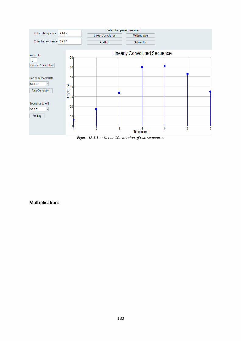
180

Figure 12.5.3.a: Linear COnvoltuion of two sequences

Multiplication:

181

Figure 12.5.3.b: Circular Convoltuion of two sequences

Addition:

Figure 12.5.3.c: Addition of two sequences

Subtraction:

182

Figure 12.5.3.d: Subtraction of two sequences

Circular Convolution:

Figure 12.5.3.e: Circular Convoltuion of two sequences

Autocorrelation of the second sequence:

183

Figure 12.5.3.f: Auto Correlation of the given sequence

Folding of the first sequence:

Figure 12.5.3.g: Folding Operation on the given sequence

12.6 UDP COMMUNICATION BETWEEN EMBED AND COMPOSE

184

The following example describes how to read UDP data in Compose Python and how the imported data can be transferred to oml using Python-oml bridge for better visualization purpose. The UDP data is written into the specified port using Embed Tool which is another Altair Product. Step1: Go to windows firewall and select Inbound rules as shown below.

Figure 12.6.a: Inbound Rules Option

Step 2: Create new rule. The following window appears. Click on “port” and select “Next”.

Figure 12.6.b: UDP Port Creation

185

Step 3: Select “UDP” and give a port number (5000) as shown below. Then click on “Next”.

Figure 12.6.c: UDP Port Creation

Step 4: Click on “Next”.

Figure 12.6.d: UDP Port Creation

186

Step 5: Click on “Next”.

Figure 12.6.e: UDP Port Creation

Step 6: Give the port name (Rxr1) and then click on “Finish”.

Figure 12.6.f: UDP Port Creation

187

Step 7: Type ipconfig in command prompt and obtain the ipv4 address as shown below.

Figure 12.6.g: IPv4 Address

Step 8: Drag and drop a UDP write block from Blocks-> Real Time->UDP Write. Give the input source sine wave of frequency 0.159 and a constant input to enable the block as shown below.

Figure 12.6.h: UDP Block in Embed

Step 9:

188

Double click on UDP write block and do the settings as shown below and click ok.

Figure 12.6.i: UDP Port Settings in Embed

Step 10: Set the system properties in Embed as shown below

Figure 12.6.j: Systems Properties Settings in Embed

Step 11:

189

Write the script in Python Compose to read the UDP data. import socket UDP_IP = "172.16.88.136" UDP_PORT = 5000 sock = socket.socket(socket.AF_INET, # Internet socket.SOCK_DGRAM) # UDP sock.bind((UDP_IP, UDP_PORT)) #while True: import array import numpy as np array1 = np.zeros((500)) for i in range (0,500): data, addr = sock.recvfrom(4096) # buffer size is 1024 bytes #print ("received message:", data) data_float = array.array('f', data) array1[i]=data_float[0] #orig_data = int.from_bytes(data,byteorder='big') print(data_float) EvalOmlFile('C:/Users/sijog/Desktop/RCI/UDP/udp_data_in_Compose.oml') %----User Defined GUI in oml to plot the data from Python using Python-oml Bridge clear all;clc; close all; global data_tcp; global data_udp; global data_serial; f = figure('position', [0.25 0.25 0.5 0.5]); %txt2 = uicontrol('Style','text','units','normalized', 'Position', [0 0.12 0.17 0.05],'String','Select Protocol:'); imshow('C:/Users/sijog/Desktop/RCI/UDP/python_udp.png','units','normalized','position', [0.3 0 0.4 0.05]); txt = uicontrol('Style','text', 'Position', [0 25 95 20],'String','Select Protocol:'); different_utility = uicontrol('Style','popup', 'String',{'Select Protocol','UDP','TCP','Serial'},'position',[0 50 120 20],'callback',@utility); function plot_types(handle, callbackdata) global data_tcp; global data_udp; global data_serial; if (isempty(data_tcp) && isempty(data_serial)) data = data_udp; end if (isempty(data_tcp) && isempty(data_udp)) data = data_serial; end if (isempty(data_udp) && isempty(data_serial)) data = data_tcp; end

190

value1 = get(handle,'value'); if value1 == 2 axes('units', 'normalized', 'position', [0.2 0.1 0.8 0.9]); plot(data); grid; title('Simple Plot'); xlabel('Time(sec)'); ylabel('Amplitude'); end if value1 == 3 axes('units', 'normalized', 'position', [0.2 0.1 0.8 0.9]); stem(data); grid; title( 'Stem Plot'); xlabel('Time(sec)'); ylabel('Amplitude'); end if value1 == 4 axes('units', 'normalized', 'position', [0.2 0.1 0.8 0.9]); bar(data); grid; title( 'Bar Plot'); xlabel('Time(sec)'); ylabel('Amplitude'); end if value1 == 5 axes('units', 'normalized', 'position', [0.2 0.1 0.8 0.9]); area(data); grid; title( 'Area Plot'); xlabel('Time(sec)'); ylabel('Amplitude'); end if value1 == 6 axes('units', 'normalized', 'position', [0.2 0.1 0.8 0.9]); loglog(data); title( 'Log-Log Plot'); xlabel('Time(sec)'); ylabel('Amplitude'); end if value1 == 7 axes('units', 'normalized', 'position', [0.2 0.1 0.8 0.9]); semilogy(data); title( 'Semilogy Plot'); xlabel('Time(sec)');

191

ylabel('Amplitude'); end if value1 == 8 axes('units', 'normalized', 'position', [0.2 0.1 0.8 0.9]); polar(data); title( 'Polar Plot'); xlabel('Time(sec)'); ylabel('Amplitude'); end end function utility(handle, callbackdata) global data_udp; global data_tcp; global data_serial; value1 = get(handle,'value'); if value1 == 2 data_udp = (getpythonvar('array1')); udp_ip = (getpythonvar('UDP_IP')); udp_port = (getpythonvar('UDP_PORT')); txt1 = uicontrol('Style','text', 'Position', [0 83 50 20],'String','UDP IP:'); ip = uicontrol('Style','edit','String',udp_ip,'Position',[0 105 80 25]) txt2 = uicontrol('Style','text', 'Position', [0 150 80 20],'String','UDP PORT:'); port = uicontrol('Style','edit','String',num2str(udp_port),'Position',[0 175 50 25]) different_plots = uicontrol('Style','popup', 'String',{'Select Plot Type','Simple Plot','Stem Plot','Bar Plot','Area Plot','loglog Plot','Semilogy Plot','Polar Plot'},'position',[0 210 150 20],'callback',@plot_types); end if value1 == 3 data_tcp = (getpythonvar('data')); tcp_ip = (getpythonvar('TCP_IP')); tcp_port = (getpythonvar('TCP_PORT')); txt1 = uicontrol('Style','text', 'Position', [0 83 50 20],'String','TCP IP:'); ip = uicontrol('Style','edit','String',tcp_ip,'Position',[0 105 80 25]) txt2 = uicontrol('Style','text', 'Position', [0 150 80 20],'String','TCP PORT:'); port = uicontrol('Style','edit','String',num2str(tcp_port),'Position',[0 175 50 25]) different_plots = uicontrol('Style','popup', 'String',{'Select Plot Type','Simple Plot','Stem Plot','Bar Plot','Area Plot','loglog Plot','Semilogy Plot','Polar Plot'},'position',[0 210 150 20],'callback',@plot_types); end if value1 == 4 data_serial = (getpythonvar('orig_data')); serial_port= (getpythonvar('port1')); baud_rate = (getpythonvar('baud_rate')); txt1 = uicontrol('Style','text', 'Position', [0 83 65 20],'String','PORT NO:');

192

ip = uicontrol('Style','edit','String',num2str(serial_port),'Position',[0 105 80 25]) txt2 = uicontrol('Style','text', 'Position', [0 150 80 20],'String','BAUD RATE:'); port = uicontrol('Style','edit','String',num2str(baud_rate),'Position',[0 175 50 25]) different_plots = uicontrol('Style','popup', 'String',{'Select Plot Type','Simple Plot','Stem Plot','Bar Plot','Area Plot','loglog Plot','Semilogy Plot','Polar Plot'},'position',[0 210 150 20],'callback',@plot_types); end Step 12: Execute both Embed and Compose simultaneously and we can see the following GUI in Compose. You can select the protocol you have defined and GUI also displays the UDP IP, the port selected and it also gives you the option to select the type of plot required.

Figure 12.6.k: Visualization of data in COmpose through UDP port

12.7 INTERRUPT BASED SERIAL COMMUNICATION IN COMPOSE

193

Pre-Requisites

Item No Description

1 Microsoft Visual Studio 2015


3 “ToolBox Sample” Visual Studio Project from Altair

4 Arduino Software and Arduino Board

Introduction

In Telecommunication and Computer Science, serial communication is the process of

sending/receiving data in one bit at a time. It is like you are firing bullets from a machine

gun to a target… that’s one bullet at a time! The pictorial representation of serial

communication is represented below.

Figure 12.7.a: Sender-Receiver Concept in Serial communication

Serial communication can be implemented using polling method and Interrupt driven

method. Interrupt and polling are the two ways to handle events generated by the devices

that can happen at any moment while CPU is busy in executing another process. The basic

point that distinguishes Polling and Interrupt is that in polling CPU keeps on checking

I/O devices at regular interval whether it needs CPU service whereas, in interrupt, the I/O

device interrupts the CPU and tell CPU that it need CPU service.

Purpose

The purpose of this tutorial is to describe how to send sensor data from Universal GPIO

Board to Compose using Arduino board through the serial port. It provides you a class called

PortDataReceived which enables you to implement interrupt based serial

communication in your application. It also describes how one can continue using Compose

and execute operations on serial data only when it is available (pg.16).

194

Part 1 – Arduino and Universal GPIO Board

Figure 12.7.b: Arduino & GPIO Board

Step 1

GPIO board was designed to allow students or engineers to easily exercise and explore the

capabilities of the various microcontrollers with peripheral devices such as: Led’s, Buttons,

Temperature sensor and many more. Proper connections must be done between Arduino and

GPIO Board. Power the GPIO Board using the following connections.

Connect the Vin of Arduino with the Vcc of GPIO Board.

Connect GND of Arduino with GND of GPIO Board.

Connect the A0(analog in) of Arduino with SOP of GPIO Board

Create a program (shown below) in Arduino which enables you to send the sensor data from

GPIO board to your system through the serial port.

195

Figure 12.7.c: Arduino Script to receive GPIO Data

196

Step 2

Select your board. You need to select the entry in the Tools > Board menu that

corresponds to your Arduino.

Figure 12.7.d: Arduino Settings

197

Step 3

Select the serial device of the Arduino board from the Tools > Port menu. This is likely

to be COM3 or higher (COM1 and COM2 are usually reserved for hardware serial ports). To

find out, you can disconnect your Arduino board and re-open the menu; the entry that

disappears from the menu. Reconnect the board and select that serial port.

Figure 12.7.d: Arduino Settings

Step 4

Now, simply click the "Upload" button in the environment. Wait a few seconds - you should

see the TX led on the board flashing. If the upload is successful, the message "Done

uploading." will appear in the status bar. (Note: If you have an Arduino Mini, NG, or other

board, you'll need to physically press the reset button on the board immediately before

clicking the upload button on the Arduino Software.)

198

Part 2 – Visual Studio Part

Step 1

Open Visual Studio 2015 and load the project/solution which is already prepared which

implements the serial communication. The interrupt based serial communication is

implemented in this tutorial by using #using "System.dll" which requires the

Common Language RunTime Support to be enabled. In-order to enable it, go to properties by

right clicking on “omlAlt” in the solution explorer. Enable the Common Language

RunTIme Support ( /clr option). Click on Apply and then press ok. /clr option creates

metadata for the application. The metadata can be consumed by other CLR applications, and

enables the application to consume types and data in the metadata of other CLR components.

Figure 12.7.e: Visual Studio Properties Settings

Step 2

Make sure that the Visual Studio is working in Release mode with x64 option.

Figure 12.7.f: Debug Option in Visual Studio

199

Step 3

This part of the code consists of header files, function declaration and definition of user

defined function name. In addition to the usual header files coming along with the Altair tool

box sample, #include “C:\Users\sijog\Desktop\Serial Communication -Final\serial_read.h” is

added which constitutes the interrupt based code for serial communication.

Figure 12.7.g: C++ Script

The following function triggers the interrupt based concept which is defined under the

reference class PortDataReceived. The function takes two inputs. One is Baudrate (type:

scalar) and the other one is COM port name ( type: string). These inputs must be given from

the Compose.

Figure 12.7.h: C++ script to receive data

200

The reference class is defined in serial_read.h which contains the definition for interrupt based communication. This makes use of two additional header files #using "System.dll" and #include <fstream>. 'gcnew' allocates memory for a managed type (reference or value type) and deallocated by using garbage collection. Baud rate is defined by the user. Parity is set None and stop bits and data bits are set to one and 8 respectively. These values must be set properly in-order to have an effective communication with the hardware.

Figure 12.7.i: Parity, baud rate and stop bit settings

When handshaking is used, the device connected to the Serial Port object is instructed to stop

sending data. When there is at least (ReadBufferSize-1024) bytes in the buffer, Request to

Send (RTS) signal is enabled during serial communication. Default is false

Figure 12.7.j: Handshaking settings and serial port opening

201

The interrupt concept is defined in DataReceiveHandler function (shown below).

Whenever there is an incoming data stream, it is then appended to a text file named

‘myfile’.

Figure 12.7.k: To append the received data into a text file

The readdata function defined below is used to read the incoming data which is stored in

the text file. The function reads the data from the text file and then exported to Compose for

displaying purpose and further manipulations.

Figure 12.7.l: To transfer the received data into Compose

202

The following snapshot shows a part of the data stream which is stored in the text file. Since

the entire data stream is stored in a text file, one could continue using compose and execute

on serial only when the user requires it for further processing. The user just wants to call the

interrupt function from Compose to enable saving the data into the text file.

Figure 12.7.m: Received Data

The closeport function is used to close the port which is previously opened for receiving

data from the Arduino Board. The function takes comport name as an input (type:string).

Figure 12.7.n: To close the port

203

The function isemptyf is defined to know whether any data is arrived through the serial

port. The function must be called from Compose. This function returns the string “No data” if

data is not arrived and returns “Data Arrived” if data is arrived through the serial port.

Figure 12.7.o: To identify the data is received or not

Step 4

From the option, ‘Build’, select ‘build solution’.

Select the path of the DLL file which has come in the output window and copy the path

of the dll file as shown below.

Figure 12.7.p: dll generation in Compose

Part 3 – Compose Part

Once the DLL is built it is turn now to import it in sT Compose. Open sT Compose and

using the command ‘addToolbox’ in the command line include the full path to the dll

as shown in the snapshot below. Once done you could pass the inputs to the functions

to check for correctness.

204

Call the function and check the results. Steps from 1 are illustrated below.

Adding toolbox to Compose

Figure 12.7.q: Adding Toolbox to Compose

Generation of GUI part

Figure 12.7.r: Creation of GUI to display data

GUI part for filter design

Figure 12.7.s: Creation of GUI for filter design

GUI part for FFT

Figure 12.7.t: Creation of GUI for FFT

205

To close the port

Result:

Original Data

Figure 12.7.u: Visualization of data in COmpose obtained from GPIO board

Filtered Signal

Figure 12.7.v: Filtered Data

206

FFT of the signal

Figure 12.7.w: FFT of the Filtered Data

How user can continue using Compose and execute on serial data only when it is available?

Reference the dll to the addToolbox function (shown below)

Call the Interrupt function along with the baud rate and comport name.

Call the function isemptyf()

The function checks for serial data and if it is available, it displays “Data Arrived”. If there is

no incoming data stream, it will display “No Data”. If the data is available, the user can call

the function readdata() for further analysis.

Figure 12.7.x: To check whether data is arrived or not

a guide to solidthinking compose · 2018-05-04 · will find yourself at a higher level of...

Documents