a harmonic balance approach for large-scale problems in

A Harmonic Balance Approach for Large-Scale Problems in Nonlinear Structural Dynamics

Allen R LaBryer, PhD Candidate Peter J Attar, Assistant Professor University of Oklahoma Aerospace and Mechanical Engineering 2010 Oklahoma Supercomputing Symposium

LaBryer 10/06/2010 University of Oklahoma

Introduction

  Time-periodic phenomena are abundant in nature   Can be analyzed experimentally or numerically   Traditional approach to numerical simulation:

  Capture the physics in language of mathematics   Partial differential equations (PDEs)   Natural oscillators tend to present themselves

as nonlinear dynamical systems   Discretize the governing equations in space

  Finite element method (FE) for structures   Temporal discretization

  Time-marching methods (Newmark, HHTα)   Computationally expensive; transient effects   Efficient alternatives exist (harmonic balance)

2

Introduction Numerical method - HDHB approach - Key features - FE implementation Application - Plunging 1D string - 2D dragonfly wing - Oscillating 3D airfoil Conclusions


Introduction

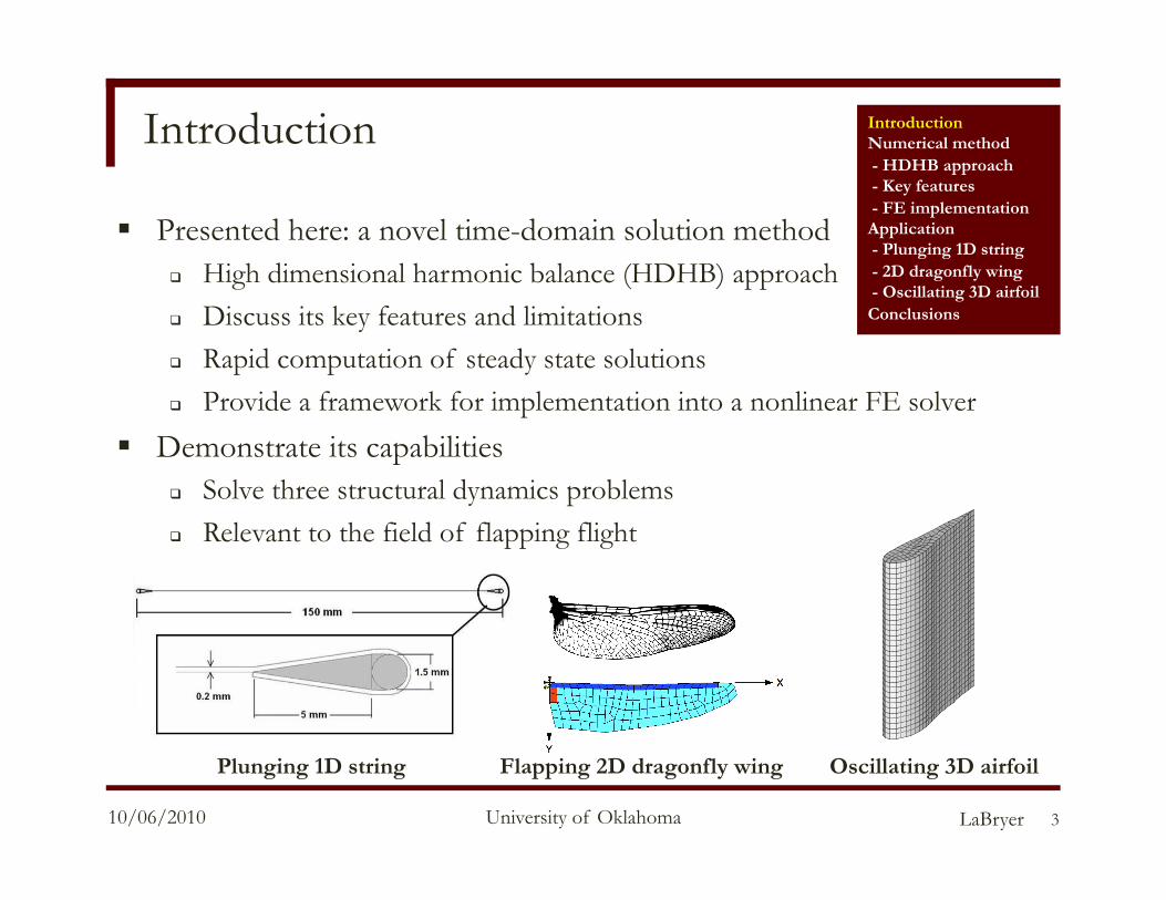
  Presented here: a novel time-domain solution method   High dimensional harmonic balance (HDHB) approach   Discuss its key features and limitations   Rapid computation of steady state solutions   Provide a framework for implementation into a nonlinear FE solver

  Demonstrate its capabilities   Solve three structural dynamics problems   Relevant to the field of flapping flight

3

X Y

Z

Plunging 1D string Flapping 2D dragonfly wing Oscillating 3D airfoil



Harmonic balance theory

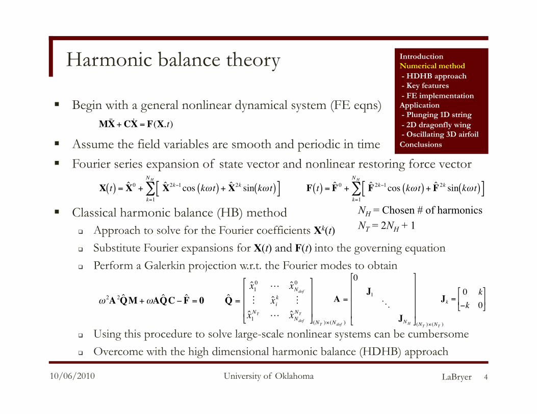
  Begin with a general nonlinear dynamical system (FE eqns)

  Assume the field variables are smooth and periodic in time   Fourier series expansion of state vector and nonlinear restoring force vector

  Classical harmonic balance (HB) method   Approach to solve for the Fourier coefficients Xk(t)   Substitute Fourier expansions for X(t) and F(t) into the governing equation   Perform a Galerkin projection w.r.t. the Fourier modes to obtain

  Using this procedure to solve large-scale nonlinear systems can be cumbersome   Overcome with the high dimensional harmonic balance (HDHB) approach

4

€

M˙ ̇ X + C ˙ X = F(X,t)

€

X t( ) = ˆ X 0 + ˆ X 2k−1 cos kω t( ) + ˆ X 2k sin kω t( )[ ]k=1

NH

∑

€

F t( ) = ˆ F 0 + ˆ F 2k−1 cos kω t( ) + ˆ F 2k sin kω t( )[ ]k=1

NH

∑

NH = Chosen # of harmonics

€

ω 2A 2 ˆ Q M +ωA ˆ Q C− ˆ F = 0

€

ˆ Q =ˆ x 1

0 ˆ x Ndof

0

ˆ x ik

ˆ x 1NT ˆ x Ndof

NT

⎡

⎣

⎢ ⎢ ⎢

⎤

⎦

⎥ ⎥ ⎥

(NT )×(Ndof )

€

A =

0J1

JNH

⎡

⎣

⎢ ⎢ ⎢ ⎢

⎤

⎦

⎥ ⎥ ⎥ ⎥ (NT )×(NT )

€

Jk =0 k−k 0⎡

⎣ ⎢

⎤

⎦ ⎥


NT = 2NH + 1


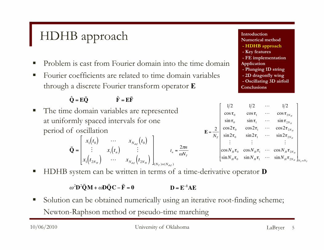
HDHB approach

  Problem is cast from Fourier domain into the time domain

  Fourier coefficients are related to time domain variables through a discrete Fourier transform operator E

  The time domain variables are represented at uniformly spaced intervals for one period of oscillation

  HDHB system can be written in terms of a time-derivative operator D

  Solution can be obtained numerically using an iterative root-finding scheme; Newton-Raphson method or pseudo-time marching

5

€

ω 2D2 ˜ Q M +ωD ˜ Q C− ˜ F = 0

€

D = E−1AE

€

˜ Q =x1 t0( ) xNdof

t0( ) xi tn( )

x1 t2NH( ) xNdoft2NH( )

⎡

⎣

⎢ ⎢ ⎢

⎤

⎦

⎥ ⎥ ⎥

(NT )×(Ndof )

€

tn =2πnωNT

€

E =2NT

1 2 1 2 1 2cosτ 0 cosτ1 cosτ 2NH

sinτ 0 sinτ1 sinτ 2NH

cos2τ 0 cos2τ1 cos2τ 2NH

sin2τ 0 sin2τ1 sin2τ 2NH

cosNHτ 0 cosNHτ1 cosNHτ 2NH

sinNHτ 0 sinNHτ1 sinNHτ 2NH

⎡

⎣

⎢ ⎢ ⎢ ⎢ ⎢ ⎢ ⎢ ⎢ ⎢ ⎢

⎤

⎦

⎥ ⎥ ⎥ ⎥ ⎥ ⎥ ⎥ ⎥ ⎥ ⎥ NT ×NT

€

ˆ Q = E ˜ Q

€

ˆ F = E ˜ F



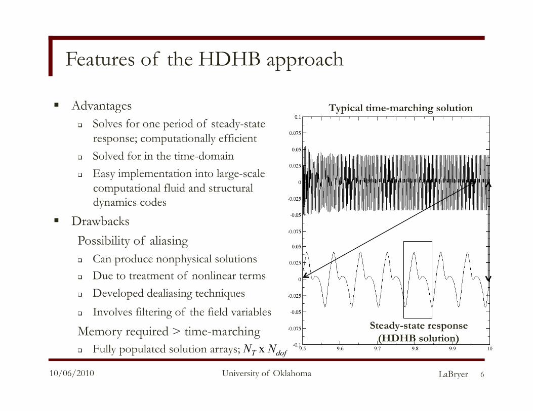
Features of the HDHB approach

  Advantages   Solves for one period of steady-state

response; computationally efficient   Solved for in the time-domain   Easy implementation into large-scale

computational fluid and structural dynamics codes

  Drawbacks

Possibility of aliasing

  Can produce nonphysical solutions   Due to treatment of nonlinear terms   Developed dealiasing techniques

  Involves filtering of the field variables

Memory required > time-marching   Fully populated solution arrays; NT x Ndof

6

Steady-state response (HDHB solution)

Typical time-marching solution


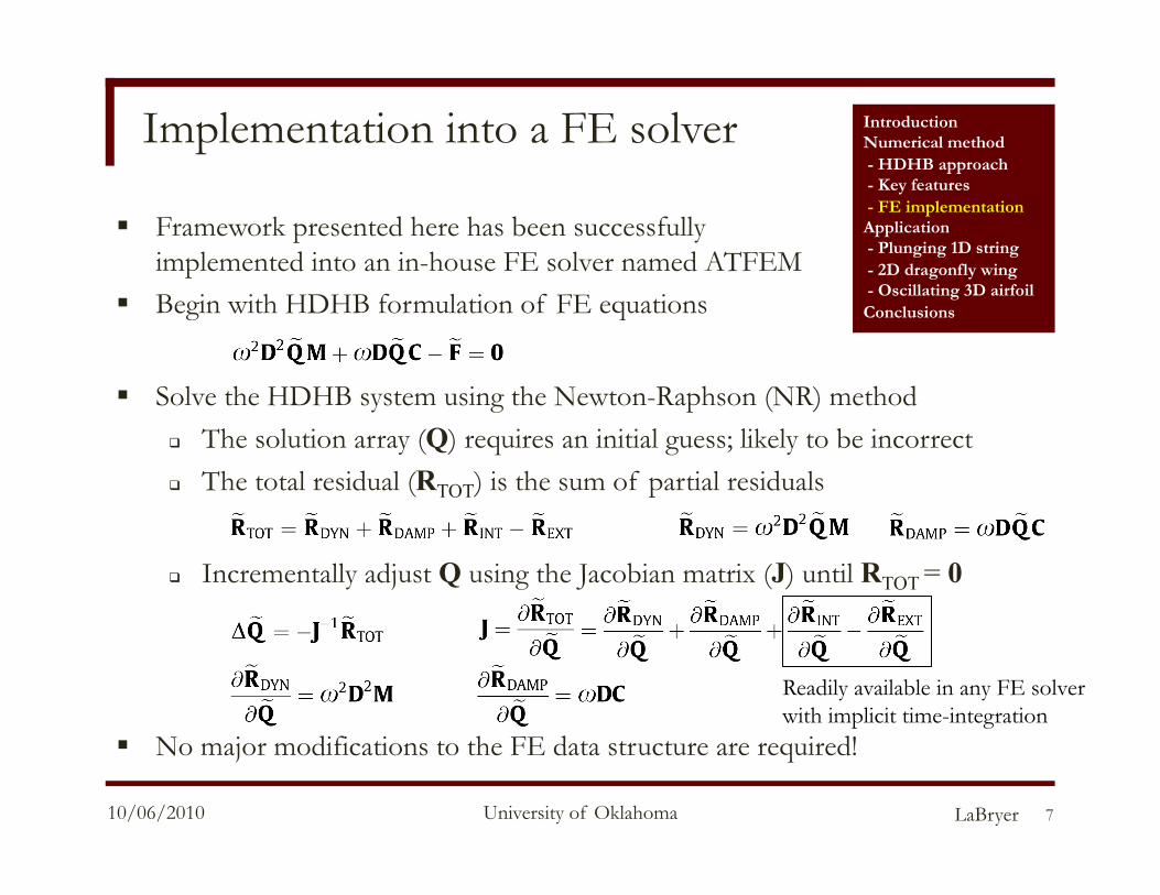
Implementation into a FE solver

  Framework presented here has been successfully implemented into an in-house FE solver named ATFEM

  Begin with HDHB formulation of FE equations

  Solve the HDHB system using the Newton-Raphson (NR) method   The solution array (Q) requires an initial guess; likely to be incorrect   The total residual (RTOT) is the sum of partial residuals

  Incrementally adjust Q using the Jacobian matrix (J) until RTOT = 0

  No major modifications to the FE data structure are required!

7


Readily available in any FE solver with implicit time-integration


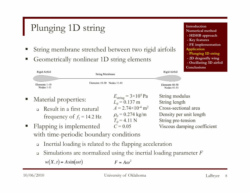
Plunging 1D string

  String membrane stretched between two rigid airfoils   Geometrically nonlinear 1D string elements

  Material properties:   Result in a first natural

frequency of f1 = 14.2 Hz

  Flapping is implemented with time-periodic boundary conditions   Inertial loading is related to the flapping acceleration   Simulations are normalized using the inertial loading parameter F

8

€

w X, t( ) = Asin ω t( )

€

F = Aω 2

Estring = 3×105 Pa String modulus L0 = 0.137 m String length A = 2.74×10-4 m2 Cross-sectional area ρ0 = 0.274 kg/m Density per unit length T0 = 4.11 N String pre-tension C = 0.05 Viscous damping coefficient



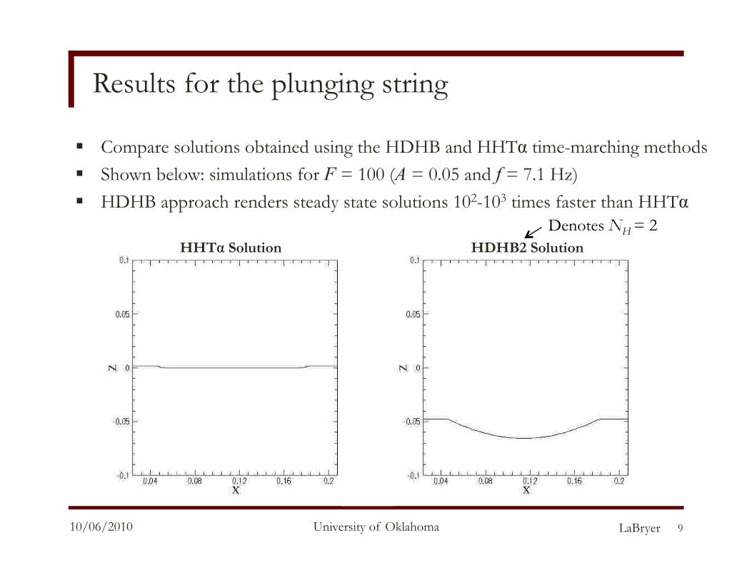
Results for the plunging string

9

HHTα Solution HDHB2 Solution

  Compare solutions obtained using the HDHB and HHTα time-marching methods   Shown below: simulations for F = 100 (A = 0.05 and f = 7.1 Hz)   HDHB approach renders steady state solutions 102-103 times faster than HHTα

Denotes NH = 2


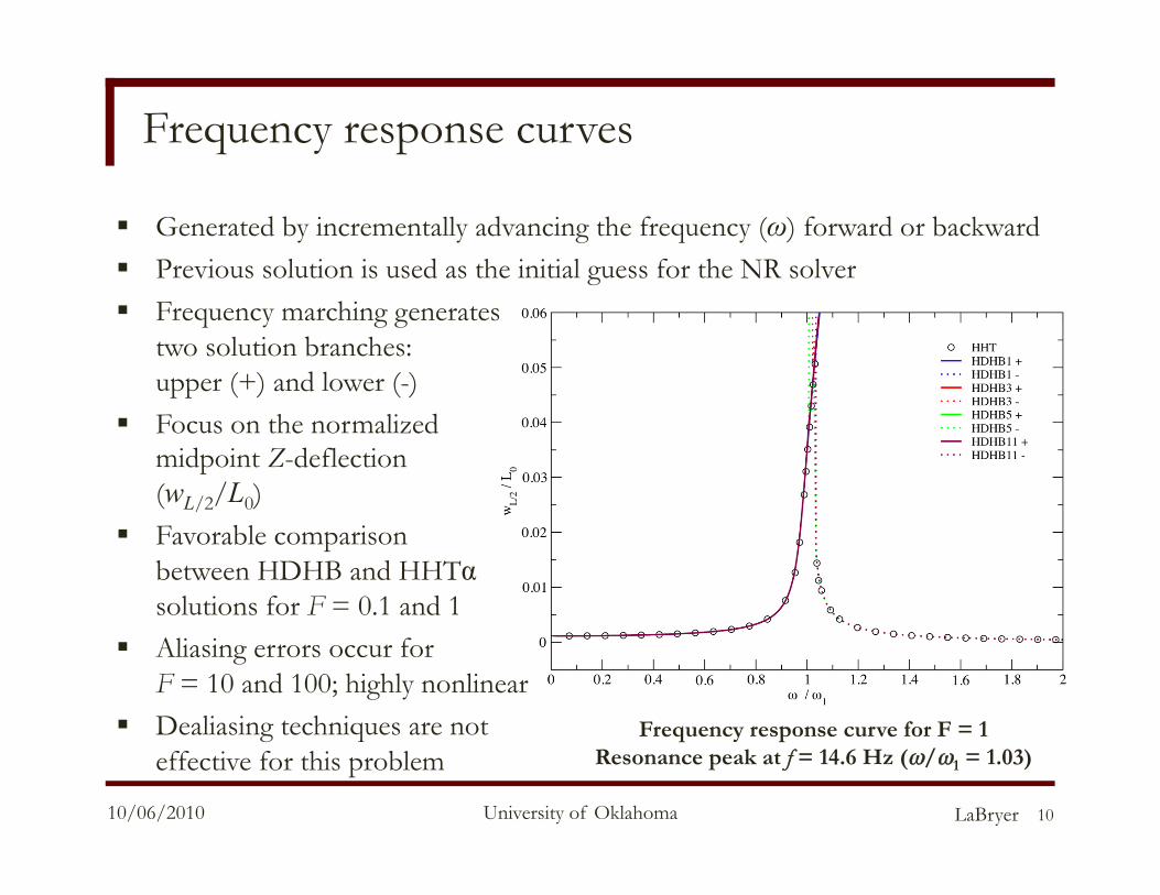
Frequency response curves

  Generated by incrementally advancing the frequency (ω) forward or backward   Previous solution is used as the initial guess for the NR solver   Frequency marching generates

two solution branches: upper (+) and lower (-)

  Focus on the normalized midpoint Z-deflection (wL/2/L0)

  Favorable comparison between HDHB and HHTα solutions for F = 0.1 and 1

  Aliasing errors occur for F = 10 and 100; highly nonlinear

  Dealiasing techniques are not effective for this problem

10

Frequency response curve for F = 1 Resonance peak at f = 14.6 Hz (ω/ω1 = 1.03)


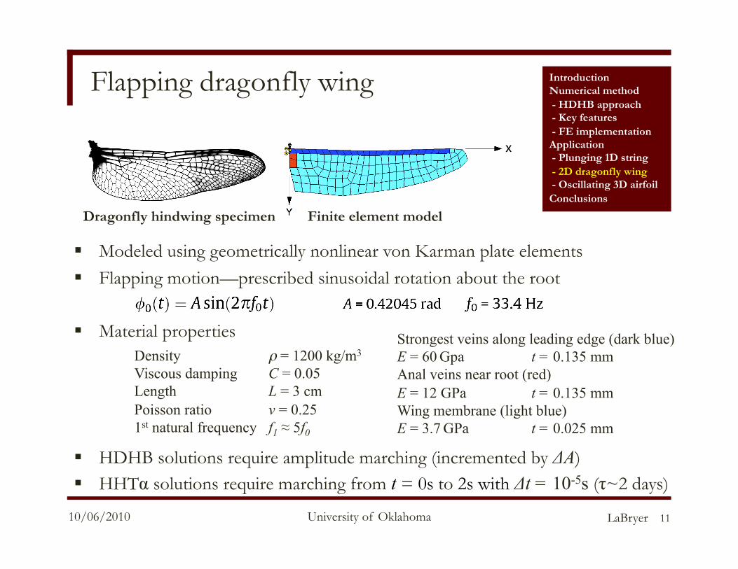
Flapping dragonfly wing

  Modeled using geometrically nonlinear von Karman plate elements   Flapping motion—prescribed sinusoidal rotation about the root

  Material properties

  HDHB solutions require amplitude marching (incremented by ΔA)   HHTα solutions require marching from t = 0s to 2s with Δt = 10-5s (τ~2 days)

11


Dragonfly hindwing specimen Finite element model

Strongest veins along leading edge (dark blue) E = 60 Gpa t = 0.135 mm Anal veins near root (red) E = 12 GPa t = 0.135 mm Wing membrane (light blue) E = 3.7 GPa t = 0.025 mm

Density ρ = 1200 kg/m3

Viscous damping C = 0.05 Length L = 3 cm Poisson ratio ν = 0.25 1st natural frequency f1 ≈ 5f0


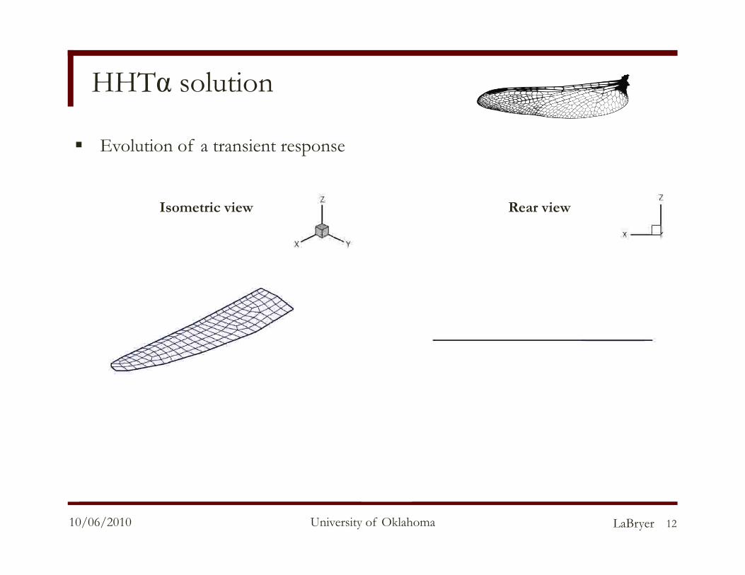
HHTα solution

12

Rear view Isometric view

  Evolution of a transient response


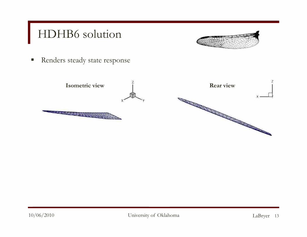
HDHB6 solution

13

Isometric view Rear view

  Renders steady state response


10-5 10-4 10-3 10-2 10-1 100 101 102

!"

0.011

0.012

0.013

0.014

0.015

0.016

0.017

0.018

wL

[m]

HDHBHHT#STEADY-STATELINEAR HDHB1

NH=1NH=2

NH=3NH=4 NH=5 NH=6

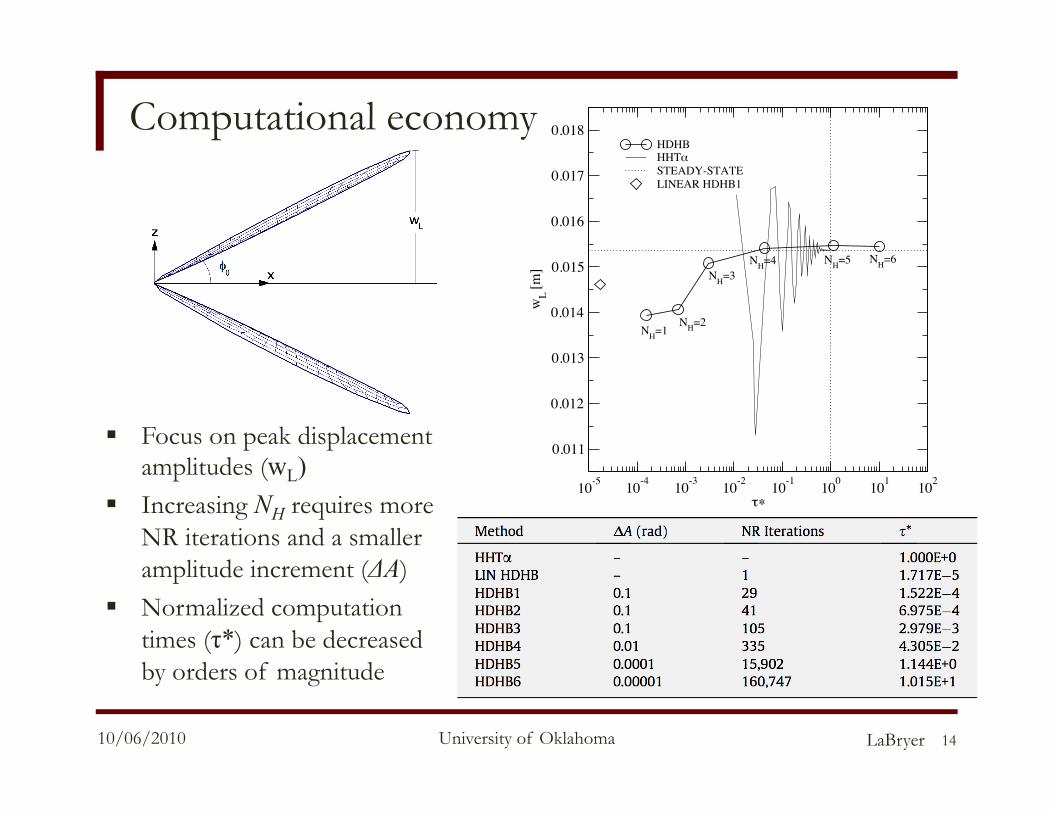
Computational economy

14

  Focus on peak displacement amplitudes (wL)

  Increasing NH requires more NR iterations and a smaller amplitude increment (ΔA)

  Normalized computation times (τ*) can be decreased by orders of magnitude


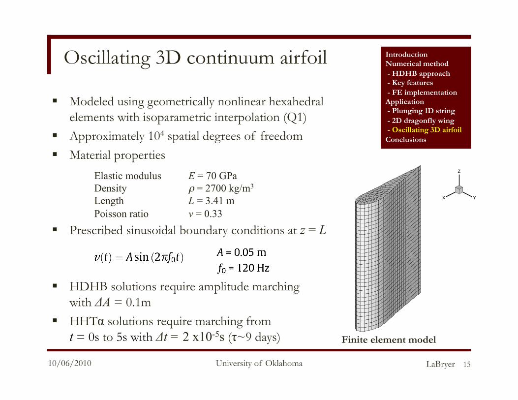
Oscillating 3D continuum airfoil

  Modeled using geometrically nonlinear hexahedral elements with isoparametric interpolation (Q1)

  Approximately 104 spatial degrees of freedom   Material properties

  Prescribed sinusoidal boundary conditions at z = L

  HDHB solutions require amplitude marching with ΔA = 0.1m

  HHTα solutions require marching from t = 0s to 5s with Δt = 2 x10-5s (τ~9 days)

15

X Y

Z


Finite element model

Elastic modulus E = 70 GPa Density ρ = 2700 kg/m3

Length L = 3.41 m Poisson ratio ν = 0.33


0 0.2 0.4 0.6 0.8 1t/T

0

0.2

0.4

0.6

0.8

1

!1 [GPa]

HDHB6HHT"

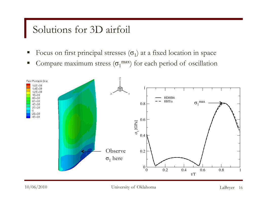
Solutions for 3D airfoil

16

  Focus on first principal stresses (σ1) at a fixed location in space   Compare maximum stress (σ1

max) for each period of oscillation

σ1max

Observe σ1 here


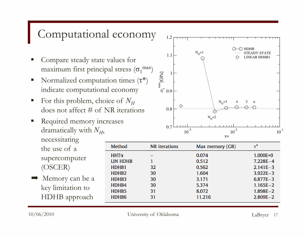
Computational economy

  Compare steady state values for maximum first principal stress (σ1

max)   Normalized computation times (τ*)

indicate computational economy   For this problem, choice of NH

does not affect # of NR iterations   Required memory increases

dramatically with NH, necessitating the use of a supercomputer (OSCER)

➡  Memory can be a key limitation to HDHB approach

17

10-3 10-2 10-1

!"

0.7

0.8

0.9

1

1.1

1.2

#1m

ax[G

Pa]

HDHBSTEADY-STATELINEAR HDHB1

NH=1

NH=2

NH=3 54 6


Conclusions

  Advantages of HDHB approach   Allows for rapid computation of steady state solutions for

time-periodic problems   Can be orders of magnitude faster than time-marching   Easy implementation into computational fluid and structural dynamics codes   No major changes need to be made to the existing FE data structure

  Drawbacks   Aliasing may occur, especially for highly nonlinear problems;

Dealiasing techniques have been developed   More memory is required compared to time-marching schemes;

May become an issue for large-scale problems

  Future research   Investigate more efficient ways to solve the HDHB system of equations

(other than the standard NR method presented here)   Coupling HDHB solvers for multiphysics problems, i.e., aeroelastic problems

18



References

19

Presentation adapted from A. LaBryer and P. J. Attar. A Harmonic Balance Approach for Large-Scale Problems in Nonlinear Structural Dynamics. Journal of Computers and Structures, 88 (17-18) (2010) 1002-1017.


References

20

a harmonic balance approach for large-scale problems in

Documents