a high-order unifying discontinuous formulation for the

Math. Model. Nat. Phenom.Vol. 6, No. 3, 2011, pp. 28-56

DOI: 10.1051/mmnp/20116302

A High-Order Unifying Discontinuous Formulationfor the Navier-Stokes Equations on 3D Mixed Grids

T. Haga, H. Gao and Z. J. Wang∗

Department of Aerospace Engineering and CFD Center, Iowa State University, 50011 Ames, USA

Abstract. The newly developed unifying discontinuous formulation named the correction pro-cedure via reconstruction (CPR) for conservation laws is extended to solve the Navier-Stokesequations for 3D mixed grids. In the current development, tetrahedrons and triangular prismsare considered. The CPR method can unify several popular high order methods including the dis-continuous Galerkin and the spectral volume methods into a more efficient differential form. Byselecting the solution points to coincide with the flux points, solution reconstruction can be com-pletely avoided. Accuracy studies confirmed that the optimal order of accuracy can be achievedwith the method. Several benchmark test cases are computed by solving the Euler and compress-ible Navier-Stokes equations to demonstrate its performance.

Key words: high-order, mixed unstructured grids, Navier-Stokes equations, discontinuous Galerkin,spectral collocation, finite differenceAMS subject classification: 65M70, 76M20, 76M22

1. IntroductionAdvantages of high-order methods are well recognized in the computational fluid dynamics (CFD)community especially for aeroacoustic noise predictions, vortex dominated flows, large eddy sim-ulation and direct numerical simulation (DNS) of turbulent flows. Since the truncation error of ahigh-order method decreases more rapidly than that of a lower order method when the solution is

∗Corresponding author. E-mail: [email protected]

28

Article published by EDP Sciences and available at http://www.mmnp-journal.org orhttp://dx.doi.org/10.1051/mmnp/20116302

http://publications.edpsciences.org/

http://www.mmnp-journal.org

http://dx.doi.org/10.1051/mmnp/20116302

T. Haga et al. A High-Order Unifying Discontinuous Formulation on 3D Mixed Grids

sufficiently smooth, the more stringent the accuracy requirement is, the more efficient a high-ordermethod becomes in computational cost. For the practical use in industries, lower order (1st or 2nd)unstructured grid methods are usually employed for the reason of superior geometrical flexibilityand robustness. However, these methods are likely too dissipative to capture small vortex struc-tures in turbulent flows. Also, as is reported in the Drag Prediction Workshop (DPW), it will beprohibitively expensive to reach the grid converged solution even in the steady RANS simulationfor a relatively simple configuration due to the slow convergence rate. Increased prediction accu-racy is often required for many aerodynamic problems with both complex physics and geometry,such as helicopter blade vortex interactions, flow over high lift devices, and aero-acoustic noisegenerated by the landing gear.

In the past decades, there has been significant progress in developing high-order methods ca-pable of solving the Navier-Stokes (NS) equations on unstructured grids. For compressible flowcomputations in aerospace applications, the discontinuous Galerkin (DG) method [1, 2, 4, 5, 7, 28,30, 42] has attracted intensive interest. One particular feature of the DG method is the discontinu-ous solution space of high-order approximations for each element, which allows the scheme to bevery flexible in dealing with complex configuration and in accommodating solution based adap-tations. Other methods assuming element-wise discontinuous solution are staggered-grid (SG)multi-domain spectral method [20], spectral volume (SV) [12, 14, 24, 39, 43, 46, 47, 48] and spec-tral difference (SD) [22, 23, 27, 40] methods. Another notable feature that is common among thesemethods is the use of one of the Riemann solvers [18, 21, 29, 31, 32] to compute unique fluxes atelement interfaces to incorporate “upwinding” characteristics of wave propagation, similar to theGodunov type finite volume method [11, 41]. The main difference among these methods lies inhow the governing equations are discretized and the degrees-of-freedom (DOFs) are chosen andupdated. The DG method is based on the weighted residual form. Various types of DG schemes arederived with different choice of DOFs. Depending on how the DOFs are defined, DG schemes canbe further divided into modal and nodal approaches. The SV method is discretized in the integralform similar to the finite volume method and the DOFs are always the sub-cell or control volume(CV) averages. The SG/SD method is based on the differential form without any integration andthe DOFs are chosen as the nodal values within each element. More comprehensive reviews ofthese methods are given in [44].

Recently, a novel formulation named correction procedure via reconstruction (CPR) was de-veloped by Huynh [16, 17] for 1D conservation laws, and extended to simplex and hybrid meshesby Wang and Gao [45]. The CPR method is based on a nodal differential form, with an element-wise discontinuous polynomial solution space. The solution polynomial is interpolated from thesolutions at a set of solution points. This formulation has some remarkable properties. The frame-work is easy to understand, efficient to implement and recovers several known methods such as theDG, SG or the SV/SD methods. Furthermore, by choosing the solution points to coincide with theflux points, the reconstruction of solution polynomials to calculate the residual can be completelyavoided. The DG scheme derived through the CPR framework is probably the simplest and mostefficient amongst all DG formulations since explicit integrations are avoided. In a recent study [9],the CPR method has been extended to the Navier-Stokes equations on 2D mixed meshes. Thesesuccessful developments laid a solid foundation for its efficient implementation and demonstration

29


on arbitrary grids in 3D.Hybrid elements such as hex, prism, pyramid and tetrahedron will provide great geometrical

flexibility for practical problems in 3D. In particular, for high Reynolds number flows in aero-dynamic applications, prismatic cells have the advantages in accuracy and computational cost toresolve boundary layers near the wall. There have been several attempts to develop the DG methodon arbitrary grid elements. In [33] different types of elements such as hex, prism and pyramidare projected onto a reference cube using collapsed Cartesian coordinates and hierarchical basisfunctions over the cube are used. Luo et.al. [25] presented a different approach based on theTaylor series expansion at the center of arbitrary element. Gassner et.al. [10] used polymorphicnodal element in the modal based formulation to reduce the cost of numerical integrations. How-ever one obvious shortcoming of these formulations is the high computational cost of the surfaceand volume integrations coming from the weighted residual formulation. Another difficulty is thetreatment of curvilinear boundary elements. In the CPR method, curvilinear boundary elementsare dealt with the same mapping technique as finite element method (FEM). The Jacobian and met-rics of the transformation matrix are stored only at the solution points and there is no additionalimplementation for a surface or volume integration. The simple formulation of the CPR methodis expected to alleviate the computational costs and facilitate the efficient treatment of curved wallboundaries.

In the present study, we develop the CPR for solving the Euler and Navier-Stokes equationson 3D mixed meshes. Tetrahedral and prismatic elements are considered in the present study withthe intention to resolve viscous boundary layer flows efficiently. The remainder of this article isorganized as follows. The basic formulation of the CPR method is described in the next section.In Section 3, The discretization of the compressible Navier-Stokes equations is derived in theCPR framework. Subsequently, we discuss how to implement the CPR method efficiently in eachparticular element with curvilinear geometry in Section 4. Section 5 presents the computationalresults for several benchmark problems, including accuracy studies on mixed unstructured grids.Conclusions for the present study and possible future works are summarized in Section 6.

2. Review of the Correction Procedure via Reconstruction For-mulation

We first review the CPR formulation for a hyperbolic conservation law, which is written as

∂Q

∂t+ ∇ ⋅ F (Q) = 0, (2.1)

with suitable initial and boundary conditions. Q is the vector of conserved variables, and F is theflux vector. Assume that the computational domain is discretized into N non-overlapping elements{Vi}. The weighted residual form of Eq. (2.1) on element Vi can be derived through multiplying

30


Eq. (2.1) by an arbitrary weighting or test function W and integrating over Vi,∫

Vi

∂Q

∂tWdV +

∫

∂Vi

WF (Q) ⋅ ndS −∫

Vi

∇W ⋅ F (Q)dV = 0. (2.2)

Let Qℎi be an approximate solution to Q on element Vi. We assume that the solution belongs to

the space of polynomials of degree k or less, i.e., Qℎi ∈ P k(Vi), within each element without

continuity requirement across element interfaces. Then, we require that the numerical solution Qℎi

must satisfy Eq. (2.2), i.e.,∫

Vi

∂Qℎi

∂tWdV +

∫

∂Vi

WF (Qℎi ) ⋅ ndS −

∫

Vi

∇W ⋅ F (Qℎi )dV = 0. (2.3)

Because the approximated solution is in general discontinuous across element interfaces, the fluxesat the interfaces are not well defined. To evaluate a unique flux and also to provide element cou-pling, a common Riemann flux is used to replace the normal flux, i.e.,

F n(Qℎi ) ≡ F (Qℎ

i ) ⋅ n ≈ F ncom(Q

ℎi , Q

ℎi+, n), (2.4)

where Qℎi+ is the solution from outside of the current element Vi. Thus, Eq. (2.3) becomes

∫

Vi

∂Qℎi

∂tWdV +

∫

∂Vi

WF ncomdS −

∫

Vi

∇W ⋅ F (Qℎi )dV = 0. (2.5)

If the space of W is chosen to be the same as the solution space, Eq. (2.5) is equivalent to theDG formulation. For the sake of a simpler formulation, we wish to eliminate the test function.Applying integration by parts to the last term of Eq. (2.5), we obtain

∫

Vi

∂Qℎi

∂tWdV +

∫

Vi

W ∇ ⋅ F (Qℎi )dV +

∫

∂Vi

W[F ncom − F n(Qℎ

i )]dS = 0. (2.6)

The last term of Eq. (2.6) can be viewed as a penalty term, i.e., penalizing the normal flux dif-ferences [F n] = F n

com − F n(Qℎi ). Let us introduce a “correction field” ±i ∈ P k(Vi), which is

determined from the following relation defining the so-called “lifting operator” for [F n].∫

Vi

W±idV =

∫

∂Vi

W [F n]dS. (2.7)

Substituting Eq. (2.7) into Eq. (2.6), we obtain∫

Vi

[∂Qℎ

i

∂t+ ∇ ⋅ F (Qℎ

i ) + ±i

]WdV = 0. (2.8)

In the present study, in order to simplify the derivation we also approximate the flux divergence bypolynomials of degree k or less. Denote Π(∇ ⋅ F (Qℎ

i )) a projection of ∇ ⋅ F (Qℎi ) to P k. If W is

selected such that a unique solution exists, Eq. (2.8) is equivalent to

∂Qℎi

∂t+Π

(∇ ⋅ F (Qℎ

i ))+ ±i = 0. (2.9)

31


i.e., Eq. (2.9) is satisfied everywhere in element Vi. With the definition of a correction field, wehave successfully reduced the weighted residual formulation to an equivalent simple differentialform. Even though we need to solve Eq. (2.7) through a volume and surface integral to define thecorrection ±i, we can circumvent the numerical quadratures in the DG algorithm which must beexact for degree 2k + 1 and 2k polynomials for the surface and volume integral.

To find the approximate solution Qℎi , let the DOFs be the solution values at a set of points

{ri,j}, named solution points (SPs). Then Eq. (2.9) must hold at the SPs, i.e.,

∂Qℎi,j

∂t+Πj

(∇ ⋅ F (Qℎ

i ))+ ±i,j = 0, (2.10)

where Πj

(∇ ⋅ F (Qℎ

i ))

denotes the values of Π(∇ ⋅ F (Qℎ

i ))

at SP j. Once the location of SPs is

defined, Qℎi and ±i can be expressed in terms of values at SPs using a Lagrange interpolation, i.e.,

Qℎi =

∑j

LSPj (ri,j)Q

ℎi,j, (2.11)

±i =∑j

LSPj (ri,j) ±i,j, (2.12)

where LSP ∈ P k are the Lagrange polynomials based on the location of SPs.To compute ±i,j , we approximate (for nonlinear conservation laws) the normal flux difference

[F n] in the RHS of Eq. (2.7) with a degree k polynomial on each interface. The interpolation canbe determined by defining flux points (FPs) as,

[F n]f ≈∑

l

LFPl (rf,l) [F

n]f,l, (2.13)

where f is an face index, and l is the FP index, and LFPl is the Lagrange interpolation polynomial

based on the FPs in a local interface coordinate. Then, if the locations of the solution and fluxpoints are specified, ±i,j can be uniquely defined by solving the linear system derived from Eq.(2.7). For simplex elements with straight faces, it can be expressed in the following formula

±i,j =1

∣Vi∣∑

f∈∂Vi

∑

l

®j,f,l[Fn]f,lSf , (2.14)

where ®j,f,l are constant coefficients independent of the solution and the shape of the simplex.

Next, we focus on how to compute Πj

(∇ ⋅ F (Qℎ

i ))

. Two approaches are developed in [45].One is the Lagrange polynomial (LP) approach which approximate the (nonlinear) flux vecter withdegree k interpolation polynomials

F (Qℎi ) ≈

∑j

LSPj (r)F (Qℎ

i,j), (2.15)

32


Then, the projection of the flux divergence is computed as

Π(∇ ⋅ F (Qℎ

i ))=

∑j

∇LSPj ⋅ F (Qℎ

i,j). (2.16)

In this case, Π(∇ ⋅ F (Qℎ

i ))

is a degree k − 1 polynomial, which also belongs to P k. Numericalexperiments indicate that there is a slight loss of accuracy with the LP approach, but it is fullyconservative [45]. Another is the chain rule (CR) approach. The divergence of the flux vector canbe computed analytically given the approximate solution using the chain rule, i.e.,

∇ ⋅ F (Qℎi,j) =

∂F (Qℎi,j)

∂Q⋅ ∇Qℎ

i,j, (2.17)

where ∂F∂Q

is composed of the flux Jacobian matrices, which can be computed analytically. Thenthe projection is approximated by the Lagrange polynomial of degree k using the flux vector di-vergence at the solution points, i.e.,

Π(∇ ⋅ F (Qℎ

i ))≈

∑j

LSPj (r)∇ ⋅ F (Qℎ

i,j). (2.18)

Numerical experiments indicate that the CR approach is much more accurate than the LP approach,at the expense of full conservation [45].

Substituting Eq. (2.14) into Eq. (2.10) we obtain the following equation

∂Qℎi,j

∂t+Πj

(∇ ⋅ F (Qℎ

i ))+

1

∣Vi∣∑

f∈∂Vi

∑

l

®j,f,l[Fn]f,lSf = 0. (2.19)

One can clearly see that this is a collocation-like formulation with penalty-like term that comesfrom the element-wise correction polynomial to provide the coupling between elements. It canbe shown that the location of SPs does not affect the numerical scheme for linear conservationlaws [40, 16]. For efficiency, the solution points are always chosen to coincide with the fluxpoints. Therefore, no data interpolation is needed for flux calculation, which further reduces thecomputational cost. Any convergent nodal sets with enough points at the element interface aregood candidates, e.g., those found in [3, 15, 49].

Finally we want to make a remark on the relationship between the CPR formulation and othermethods including DG, SV and SD methods. Starting from the weighted residual form of thegoverning equations, different formulations can be derived depending on the weighting function.For example, a nodal DG formulation is obtained by choosing weighting functions to be Lagrangepolynomials, and a SV formulation is obtained by defining weighting functions as piecewise con-stant at the sub-cells. As a result, the only difference between those schemes appears in the cor-rection coefficients. Note that there are certainly differences how to discretize the spatial termsbetween the CPR using the DG coefficients (CPR-DG) and the nodal DG FEM. The same is truefor the SV method. Nevertheless, it was numerically confirmed that the CPR-DG or CPR-SV is

33


equivalent to the DG or SV method at least for linear conservation laws in [45]. In [45], it was alsoshown that the resulting CPR scheme is fully conservative by using the correction coefficients forthe DG, SV and SD scheme if the flux divergence term is evaluated with the LP approach. In thisstudy, we choose the weighting function to be one of the Lagrange polynomials based on the SPs,i.e., Eq. (2.9) is identical to the DG formulation.

3. Discretization of the Navier-Stokes Equations

3.1. Governing EquationsThe 3D compressible Navier-Stokes equations can be written as a system of partial differentialequations in conservation form:

∂Q

∂t+ ∇ ⋅

(Fc(Q)− Fv(Q, ∇Q)

)= 0, (3.1)

where Q, Fc = (F xc , F

yc , F

zc ) and Fv = (F x

v , Fyv , F

zv ) denote the conservative state vector, the

inviscid and the viscous flux vectors, respectively, and are given by

Q =

⎛⎜⎜⎜⎜⎝

½½u½v½we

⎞⎟⎟⎟⎟⎠

, F xc =

⎛⎜⎜⎜⎜⎝

½u½u2 + p½uv½uw

(e+ p)u

⎞⎟⎟⎟⎟⎠

, F yc =

⎛⎜⎜⎜⎜⎝

½v½uv

½v2 + p½vw

(e+ p)v

⎞⎟⎟⎟⎟⎠

, F zc =

⎛⎜⎜⎜⎜⎝

½w½uw½vw

½w2 + p(e+ p)w

⎞⎟⎟⎟⎟⎠

. (3.2)

F xv =

⎛⎜⎜⎜⎜⎝

0¿xx¿xy¿xz

u¿xx + v¿xy + w¿xz − qx

⎞⎟⎟⎟⎟⎠

, F yv =

⎛⎜⎜⎜⎜⎝

0¿yx¿yy¿yz

u¿yx + v¿yy + w¿yz − qy

⎞⎟⎟⎟⎟⎠

,

F zv =

⎛⎜⎜⎜⎜⎝

0¿zx¿zy¿zz

u¿zx + v¿zy + w¿zz − qz

⎞⎟⎟⎟⎟⎠

. (3.3)

where ½ is the density, v = (u, v, w) the velocity vector, p the pressure, e the total energy per unitvolume. The viscous stress tensor can be represented as

¿ = ¹

(∇v + (∇v)T − 2

3(∇ ⋅ v)I

). (3.4)

34


where ¹ is the molecular viscosity coefficient, I is the unit tensor. The heat flux is given as

q = −cp¹

Pr∇T. (3.5)

Here, cp is the specific heat capacity at constant pressure and T is the temperature. The Prandtlnumber Pr is assumed to be a constant of 0.72 in this study. For a perfect gas, the pressure isrelated to the total energy e by

e =p

° − 1+

1

2½(u2 + v2 + w2

). (3.6)

The specific heat ratio ° is set to be a constant, 1.4 for air. The computations for solving the Eulerequations are performed by omitting the viscous flux.

3.2. CPR Formulation of the Navier-Stokes EquationsIn order to discretize the Navier-Stokes equations, we follow a mixed formulation that is commonlyused for the DG method [2, 6]. By introducing a new variable R, Eq. (3.1) is rewritten in a firstorder system as

∂Q

∂t+ ∇ ⋅

(Fc(Q)− Fv(Q, R)

)= 0, (3.7)

R = ∇Q. (3.8)

According to the CPR formulation by assuming Qℎi ∈ P k, Rℎ

i ∈ (P k, P k, P k) on discretizedelements {Vi} , we obtain

∂Qℎi,j

∂t+Πj

(∇ ⋅ Fc(Q

ℎi ))− Πv

j

(∇ ⋅ Fv(Q

ℎi , R

ℎi ))+

1

∣Vi∣∑

f∈∂Vi

∑

l

®j,f,l ([Fnc ]f,l − [F n

v ]f,l)Sf .

(3.9)

Rℎi,j = (∇Qℎ

i )j +1

∣Vi∣∑

f∈∂Vi

∑

l

®j,f,l[Q]f,lnfSf , (3.10)

where [F nc ] ≡ F n

c,com − F nc (Q

ℎi , n), [F

nv ] ≡ F n

v,com − F nv (Q

ℎi , R

ℎi , n) and [Q] ≡ Qℎ

com −Qℎi .

3.2.1. Inviscid Flux Calculation

We need to discretize the projection of the inviscid flux divergence Πj

(∇ ⋅ Fc(Q

ℎi ))

and the differ-ence of the normal inviscid flux [F n

c ] in the correction term in Eq. (3.9). To compute the inviscidflux divergence we employed the CR approach in the present study. The common inviscid fluxF nc,com can be obtained with any Riemann solver. We used the Roe flux [31] for all the cases.

35


3.2.2. Viscous Flux Calculation

In the present study, we employ the BR2 scheme [2] to discretize the viscous flux. In Eq. (3.10),the common solution Qℎ

com is simply the average of the solutions at both sides of f . The viscousflux vector at the solution points are evaluated by Fv(Q

ℎi , R

ℎi ). Then the projection of the viscous

flux divergence Πvj

(∇ ⋅ Fv(Q

ℎi , R

ℎi ))

is obtained through the LP approach instead of the CR ap-

proach. In the correction term, the common viscous flux F nv,com(Q

ℎcom, ∇Qℎ

com, n) also needs to bedetermined. Besides the common solution, we also need to define a common gradient ∇Qℎ

com onface f . The common gradient at a flux point l on f is evaluated as

∇Qℎcom

∣∣∣f,l

=1

2(∇Q−

f,l + r−f,l + ∇Q+f,l + r+f,l), (3.11)

where ∇Q−f,l and ∇Q+

f,l are the gradients of the solution from the left and right cells. r−f,l and r+f,lare the local lifting corrections to the gradients only due to the common solution on face f

r±f,l =1

∣V ±∣∑m=1

®l,f,m[Q]f,m (∓nf )Sf , (3.12)

where m is the index for the flux points on f and nf is the unit normal vector directing from left toright. Note that there is no summation over all faces of the element in Eq. (3.12) in order to assurethat the BR2 scheme maintains a compact face neighbor stencil.

4. Discretization on Mixed Grids with Curved BoundaryIt can be observed that Eq. (2.9) is valid for arbitrary types of elements besides triangles andtetrahedrons. The current development for 3D hybrid meshes accommodates two kinds of elementshapes, i.e., tetrahedron and triangular prism. Other types of element such as hexahedron andpyramid will be developed in the near future. The use of prismatic cells in addition to tetrahedralcells has the advantages in both accuracy and computational costs to resolve boundary layers nearsolid walls. In order to achieve an efficient implementation, all elements are transformed fromthe physical domain (x, y, z) into a corresponding standard element in the computational domain(», ´, ³) as shown in Fig. 1. Here we consider the transformations for the elements with curvedsides (faces and edges). The discretization for the curved elements is conducted in the same wayas the straight sided elements by applying the CPR formulation in the standard elements. In thepresent study, a quadratic triangular face is employed to represent curved wall boundaries. For thesake of computational efficiency, the quadratic representation is adopted for only one of the facesof tetrahedra attached to the wall in inviscid flows, and for only two triangular faces of prismsused in the thin layers of prism cells to assure the quality of the element shape especially in highReynolds number flows.

36


Based on a set of locations of nodes defining the shape of element, a set of shape functions canbe obtained [50]. Once the shape functions Mi(», ´, ³) are given, the transformation can be writtenas ⎡

⎣xyz

⎤⎦ =

K∑i=1

Mi(», ´, ³)

⎡⎣

xi

yizi

⎤⎦ , (4.1)

where K is the number of points used to define the physical element, (xi, yi, zi) are the Cartesiancoordinates of those points. For the transformation given in Eq. (4.1), the Jacobian matrix J takesthe following form

J =∂(x, y, z)

∂(», ´, ³)=

⎡⎣

x» x´ x³

y» y´ y³z» z´ z³

⎤⎦ . (4.2)

For a non-singular transformation, its inverse transformation must also exist, and the Jacobianmatrices are related to each other according to

∂(», ´, ³)

∂(x, y, z)=

⎡⎣

»x »y »z´x ´y ´z³x ³y ³z

⎤⎦ = J−1. (4.3)

The governing equations in the physical domain are then transformed into the computational do-main (standard element), and the transformed equations take the following form

∂Q

∂t+

∂F »

∂»+

∂F ´

∂´+

∂F ³

∂³= 0, (4.4)

whereQ = ∣J ∣QF » = ∣J ∣(»xF x + »yF

y + »zFz)

F ´ = ∣J ∣(´xF x + ´yFy + ´zF

z)

F ³ = ∣J ∣(³xF x + ³yFy + ³zF

z).

(4.5)

Let S» = ∣J ∣∇», S´ = ∣J ∣∇´ and S³ = ∣J ∣∇³ . Then we have F » = F ⋅ S», F ´ = F ⋅ S´ andF ³ = F ⋅ S³ . In our implementation, J , S», S´ and S³ are stored at the solution points. Note thathere we consider the Euler equations as the governing equations for brevity’s sake. Extending thefollowing discretization to the Navier-Stokes equations is straightforward.

4.1. Discretization on a Standard TetrahedronOn a standard tetrahedron, the CPR formulation in Eq. (2.19) can be rewritten as

∂Qℎi,j

∂t+Πj

(∇(») ⋅ F (»)(Qℎ

i ))+

1

∣V (»)∣∑

f∈∂V (»)

∑

l

®j,f,l[Fn,(»)]f,lS

(»)f = 0, (4.6)

37


ξ

η

ζ

1

1

1

0

(a)

ξ

η

ζ

1

-1

1

1

0

(b)

Figure 1: Transformation of curve boundary tetrahedral and prismatic cells to the standard ele-ments.

where superscript (») means the variables or operations evaluated on the computational domain.For example, [F n,(»)] are the normal jumps of the transformed fluxes across the faces of the standardelement. The transformed normal flux can be expressed in terms of the flux in the physical spaceas

F n,(»)∣∣f,l

= F (»)∣∣∣f,l

⋅ n(»)∣∣f

= F∣∣∣f,l

⋅ S»

∣∣∣f,l

n»∣∣f+ F

∣∣∣f,l

⋅ S´

∣∣∣f,l

n´∣f + F∣∣∣f,l

⋅ S³

∣∣∣f,l

n³∣∣f

= F∣∣∣f,l

⋅ Sn∣∣∣f,l

= F n∣f,l ∣Sn∣∣∣∣f,l,

(4.7)

where n(») = (n», n´, n³) is a unit normal vector on a straight face of the standard element, andSn is a normal vector on a face in the physical space defined as Sn = S»n

» + S´n´ + S³n

³ . Notethat in solving Eq. (4.4), Q = ∣J ∣Q are the solution unknowns, and are assumed to be degree kpolynomials in the computational domain instead of Q. As a result, the derivatives of Q should becalculated in the following way,

∂Q

∂»=

1

∣J ∣(∂(∣J ∣Q)

∂»− ∂∣J ∣

∂»Q

),∂Q

∂´=

1

∣J ∣(∂(∣J ∣Q)

∂´− ∂∣J ∣

∂´Q

),

∂Q

∂³=

1

∣J ∣(∂(∣J ∣Q)

∂³− ∂∣J ∣

∂³Q

). (4.8)

In 3D, to construct a complete polynomial of degree k, at least k(k + 1)(k + 2)/3! SPs needto be chosen. In order to achieve the most efficient implementation, SPs on edges are chosento be the Legendre-Gauss Lobatto (LGL) points. For 4th- or higher order schemes, nodes insidethe boundary triangle are chosen from [15]. For 5th- or higher order schemes, nodes inside thetetrahedron are chosen from [49]. The nodal set of the 4th-order CPR scheme is shown in Fig. 2.Note that the flux difference at a flux point corrects all solution points as shown in Eq. (4.6).

38


4.2. Discretization on Standard PrismFor a standard triangular prism, the solution polynomial can be expressed as a tensor product of a1D and 2D Lagrange polynomial, i.e.,

Qℎi (», ´, ³) =

∑m

∑j

Qℎi;j,mL

SPj (», ´)LSP

m (³), (4.9)

where Qℎi;j,m are the state variables at the solution point (j,m), with j the index in » − ´ plane

and m the index in ³ direction, LSPj (», ´) is a 2D Lagrange polynomial in the standard triangle

and LSPm (³) is a 1D Lagrange polynomial. Figure 3 shows the locations of the solution points

for k = 3. The nodal sets on the edge and the triangle are chosen in the same manner as on thetetrahedral element.

The CPR formulation for a standard prism is

∂Qℎi;j,m

∂t+Πj,m

(∇(») ⋅ F (»)(Qℎ

i ))

+1

∣V (»)Tri∣

∑

f∈∂VTri

∑

l

®j,f,l[Fn,(»)(»f,l, ´f,l, ³m)]S

(»)f

− [F ³com(»j, ´j,−1)− F ³(»j, ´j,−1)]g

′L(³m)

+ [F ³com(»j, ´j, 1)− F ³(»j, ´j, 1)]g

′R(³m) = 0,

(4.10)

The correction process is done in a decoupled manner. The third term is the correction of theflux components in » and ´ directions, which is computed on a plane with fixed ³ = ³m. Thisis nothing but the correction used in the 2D CPR method for a triangular element. In Eq. (4.10),VTri is the area of the standard triangle, Sf the length of the edge f and l the index for flux pointson f . Note that, [F n,(»)(»f,l, ´f,l, ³m)] corrects only the solution points on the triangle with fixedm instead of all solution points in the element as shown in Fig. 3(a). The last two terms denotethe correction in the ³ direction, which is evaluated with the 1D CPR method [16]. gL and gRare the correction functions for the left and right end points of the segment. The flux differenceat an end point corrects only the solution points on the segment with fixed j as shown in Fig.3(b). For prism cells, the number of solution points corrected by a flux point is smaller than theone for tetrahedral cells due to the decoupled correction procedure. Hence, the method for prismsis more efficient per DOF than for tetrahedrons. This decoupled procedure also facilitates theimplementation employing different degrees of polynomials in » − ´ and ³ directions to adaptto flow features. An attempt to employ higher order polynomials in the wall normal direction toresolve the boundary layer with coarser prism cells is shown in a later section.

In order to simplify the implementation for mixed grids, we assume the polynomial degree k tobe the same for both the tetrahedral and prismatic elements. Furthermore, the flux points along theelement interfaces are required to match each other. In the present implementation, the flux pointsare selected to be the LGL points at each edge for all tetrahedral and prismatic elements.

39


ξ

η

ζ

1

1

1

0

Figure 2: Solution points in the standard tetrahedral cell for degree k = 3 polynomial (only pointson the visible faces are shown).

5. Numerical Results

5.1. Test Cases for the Euler Equations5.1.1. Accuracy Study with Vortex Evolution Problem

To assess the order of accuracy of the developed method, the propagation of an isentropic vortexis computed with successive grid refinement. This is an idealized problem for the Euler equationsin 2D used by Shu [35]. Here we consider simple extension of this problem to the 3D domain[0, 10] × [0, 10] × [0, 10]. The mean flow is (½, u, v, w, p) = (1, 1, 1, 0, 1). An isotropic vortexis then added to the mean flow, i.e., with perturbations in u, v and temperature T = p/½, and noperturbation in entropy S = p/½°:

(±u, ±v, ±w) =²

2¼e0.5(1−r2)(−y, x, 0),

±T = −(° − 1)²2

8°¼2e1−r2 , ±S = 0,

(5.1)

where r2 = x2 + y2, x = x − 5, y = y − 5, and the vortex strength ² = 5. If the computationaldomain is infinitely big, the exact solution of the Euler equations with the above initial conditionis just the passive convection of the isentropic vortex with the mean velocity (1, 1, 0). In thenumerical simulation, we impose the exact solution on the boundaries.

The computations are carried out until t = 2 on two different types of grids, tetrahedral meshesand prismatic meshes. In generating computational grids, first an equidistant Cartesian grid ofN × N × N cells is generated for the cubic domain and each cell is further divided into sixtetrahedrons or two prisms. Three different grids are employed with N = 10, 20 and 40 for eachtype of cell. For the time integration, the 3rd-order Runge-Kutta explicit scheme [34] is used. Eventhough the order of accuracy of the temporal scheme is less than the order for the spatial scheme,

40


ξ

η

ζ

1

-1

10

(a)

ξ

η

ζ

1

-1

10

(b)

Figure 3: Solution points in the standard prism cell for degree k = 3 polynomial (only points onthe visible faces are shown). (a) shows the correction in the » and ´ derections. (b) shows thecorrecgtion in the ³ direction.

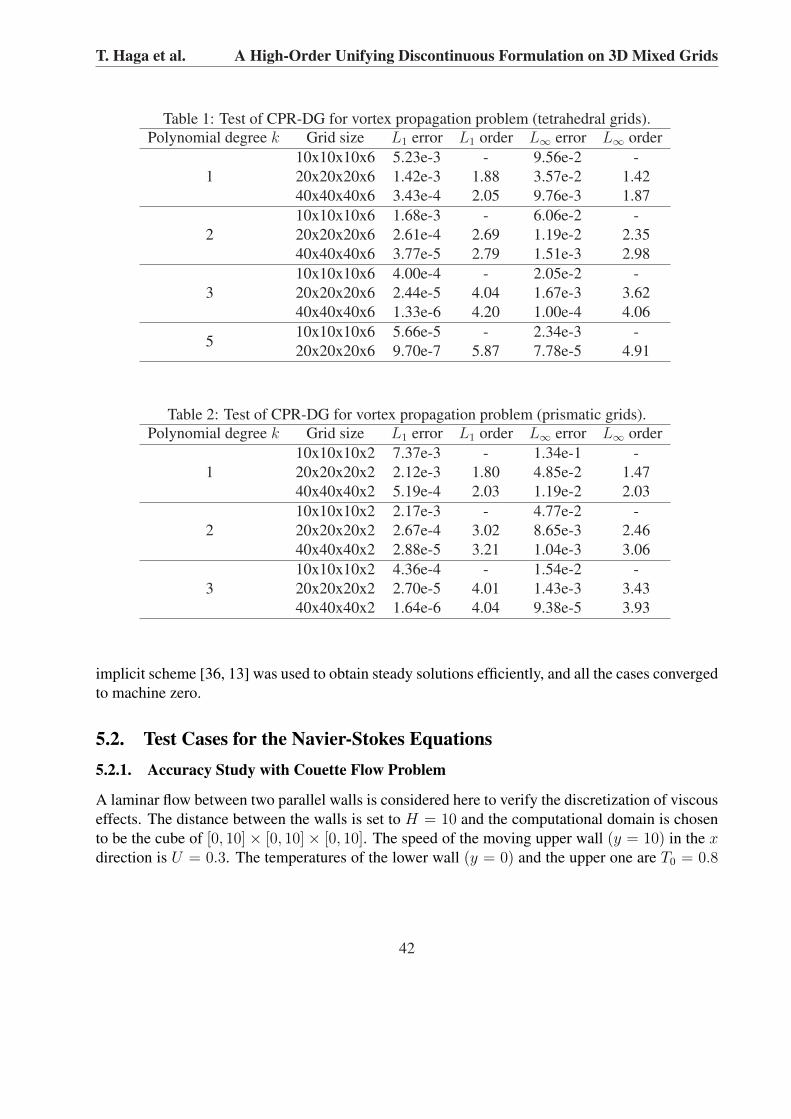
if we use a small enough timestep which does not affect the numerical solution, we can still assessthe order of convergence of the spatial operator. In this study, we fixed the timestep to 0.002 forall polynomial degree k and grids. The timestep corresponds to the CFL number of 0.138 in thefinest prism grid. We confirmed that using a smaller timestep than 0.002 almost did not change thecomputed solutions. The L1 and L∞ norms of density error at the solution points are presentedfor tetrahedral grids and prismatic grids in Tables 1 and 2, respectively. The CPR-DG methodperforms very well on both types of grid, achieving the nearly optimal order of accuracy up to6th-order in tetrahedral meshes and 4th-order in prismatic meshes.

5.1.2. Subsonic Inviscid Flow over a Sphere

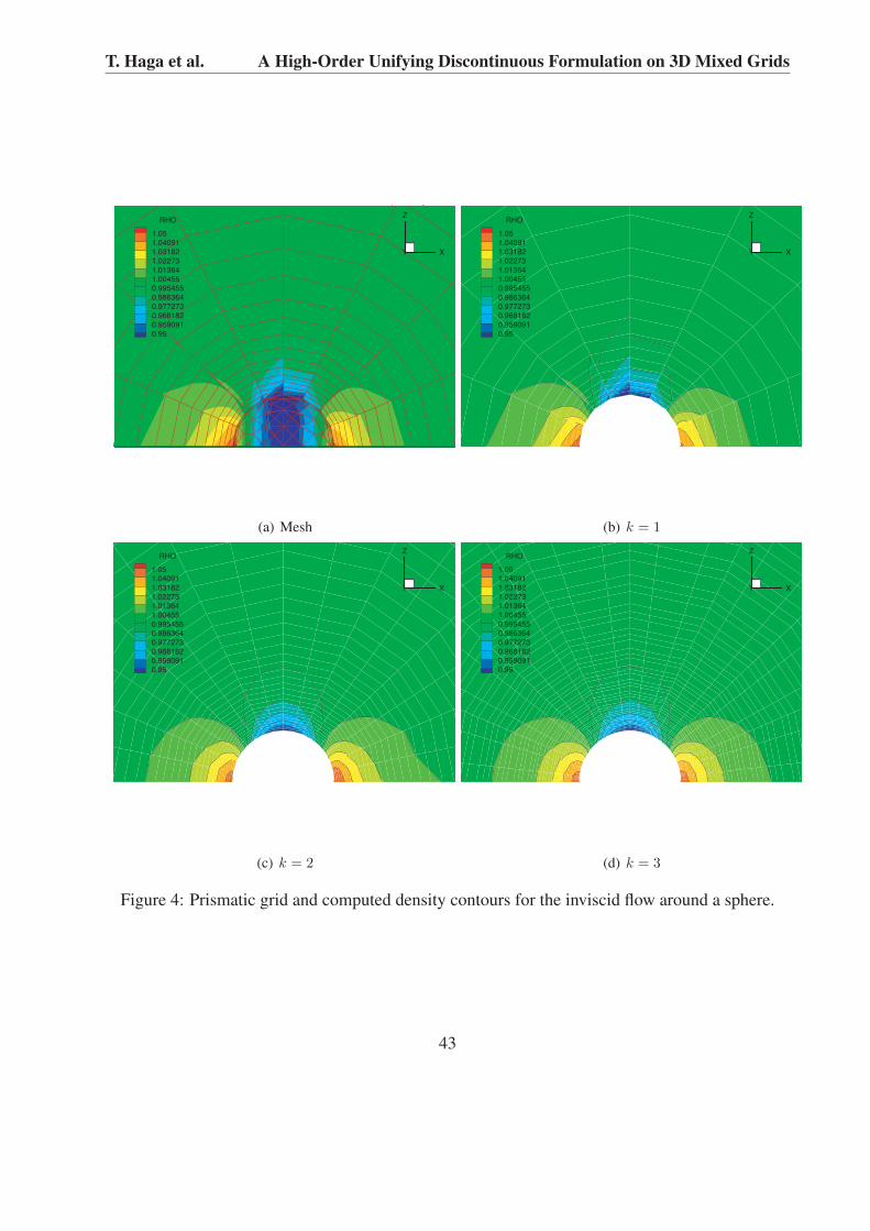
In order to verify the developed Euler solver on a mixed mesh with curved wall boundary, a typicalsteady test case of a subsonic flow around a sphere is considered. The freestream Mach numberis M = 0.3. Two computational grids are employed. One is a purely prismatic grid and theother is a mixed grid shown in Figs. 4(a) and 5(a). The mixed grid is composed of five layers ofprismatic cells around the quarter sphere and isotropic tetrahedral cells for the remaining region.To preserve the geometry of the sphere well with a relatively coarse mesh, each curved boundaryface is represented with a piecewise quadratic polynomial.

The computed density contours obtained with the 2nd- to 4th-order schemes are shown atFigs. 4(b)-(d) and Figs. 5(b)-(d). In both grids, the trends of improvement in the solution byincreasing the order of discretization are similar. The computed density contours using the 4thorder scheme appear to be perfectly symmetric without visible numerical dissipation and also quitesmooth across the interface between prismatic and tetrahedral cells. In this case, a block LU-SGS

41


Table 1: Test of CPR-DG for vortex propagation problem (tetrahedral grids).Polynomial degree k Grid size L1 error L1 order L∞ error L∞ order

110x10x10x6 5.23e-3 - 9.56e-2 -20x20x20x6 1.42e-3 1.88 3.57e-2 1.4240x40x40x6 3.43e-4 2.05 9.76e-3 1.87



510x10x10x6 5.66e-5 - 2.34e-3 -20x20x20x6 9.70e-7 5.87 7.78e-5 4.91

Table 2: Test of CPR-DG for vortex propagation problem (prismatic grids).Polynomial degree k Grid size L1 error L1 order L∞ error L∞ order




implicit scheme [36, 13] was used to obtain steady solutions efficiently, and all the cases convergedto machine zero.

5.2. Test Cases for the Navier-Stokes Equations5.2.1. Accuracy Study with Couette Flow Problem

A laminar flow between two parallel walls is considered here to verify the discretization of viscouseffects. The distance between the walls is set to H = 10 and the computational domain is chosento be the cube of [0, 10]× [0, 10]× [0, 10]. The speed of the moving upper wall (y = 10) in the xdirection is U = 0.3. The temperatures of the lower wall (y = 0) and the upper one are T0 = 0.8

42


Y X

ZRHO

1.05

1.04091

1.03182

1.02273

1.01364

1.00455

0.995455

0.986364

0.977273

0.968182

0.959091

0.95

(a) Mesh

Y X

ZRHO

1.05

1.04091

1.03182

1.02273

1.01364

1.00455

0.995455

0.986364

0.977273

0.968182

0.959091

0.95

(b) k = 1

Y X

ZRHO

1.05

1.04091

1.03182

1.02273

1.01364

1.00455

0.995455

0.986364

0.977273

0.968182

0.959091

0.95

(c) k = 2

Y X

ZRHO

1.05

1.04091

1.03182

1.02273

1.01364

1.00455

0.995455

0.986364

0.977273

0.968182

0.959091

0.95

(d) k = 3

Figure 4: Prismatic grid and computed density contours for the inviscid flow around a sphere.

43


Y X

ZRHO

1.05

1.04091

1.03182

1.02273

1.01364

1.00455

0.995455

0.986364

0.977273

0.968182

0.959091

0.95

(a) Mesh

Y X

ZRHO

1.05

1.04091

1.03182

1.02273

1.01364

1.00455

0.995455

0.986364

0.977273

0.968182

0.959091

0.95

(b) k = 1

Y X

ZRHO

1.05

1.04091

1.03182

1.02273

1.01364

1.00455

0.995455

0.986364

0.977273

0.968182

0.959091

0.95

(c) k = 2

Y X

ZRHO

1.05

1.04091

1.03182

1.02273

1.01364

1.00455

0.995455

0.986364

0.977273

0.968182

0.959091

0.95

(d) k = 3

Figure 5: Mixed grid (tetrahedrons and prisms) and computed density contours for the inviscidflow around a sphere.

44


and T1 = 0.85 respectively. The analytical solution for this case is

(u, v, w) = (y

HU, 0, 0),

T = T0 +y

H(T1 − T0) +

¹U2

2k

y

H

(1− y

H

),

p = p0, ½ =°p

T,

(5.2)

where ° is specific heat ratio and k is thermal conductivity. The static pressure is set to p0 = 1/°and the viscosity of the fluid is assumed to be ¹ = 0.01. The flow variables at boundary faces aresimply fixed to the exact solution.

Three successively refined prism grids are generated with N = 2, 4 and 8 in the same way as inthe vortex propagation case. Each cube is split into two prisms by the plane which is perpendicularto the y = 0 plane. The error norms for the BR2 formulation are presented in Table 3. The densityis used to evaluate the error. It is shown that nearly optimal order of accuracy is achieved for the2nd- to 4th-order schemes.

Table 3: Test of CPR-DG (BR2) for Couette flow problem (prismatic grids).Polynomial degree k Grid size L1 error L1 order L∞ error L∞ order




5.2.2. Laminar Boundary Layer over a Flat Plate

The laminar boundary layer over a flat plate is then computed using the CPR method. The Reynoldsnumber based on the plate length is Rex = 10, 000 and the freestream Mach number is M = 0.2.The plate length L is set to 1. The boundary layer thickness at the trailing edge is estimated bythe formula ± = 5L/

√Rex. The computational domain is selected to be (−2 ≤ x ≤ 1, 0 ≤ y ≤

100±, 0 ≤ z ≤ ±). Note that the domain size in the y-direction is chosen to be large enough notto affect the results especially in the v-velocity profiles. The freestream values are specified at theinflow boundary at x = −2 and the top boundary at y = 100±. For the lower boundary at y = 0,the symmetry conditions are used on the upwind side to the wall (−2 ≤ x ≤ 0) and the adiabaticwall conditions are imposed on the wall (0 ≤ x ≤ 1). At the outflow boundary at x = 1, only

45


static pressure is prescribed. On the side boundaries at z = 0 and ±, the symmetric conditionsare assumed. First, we generated a three dimensional Cartesian mesh. The grid cells are clusterednear the leading edge and the cell sizes are increased geometrically in both x- and y-directions. Inthe spanwise z-direction, we generate only one cell. Then we divide each hexahedral cell into twoprisms to obtain a purely prismatic grid.

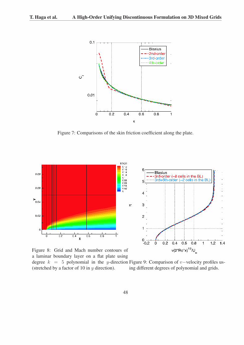
The computed u and v velocity profiles are compared with the Blasius’s solution in Fig. 6.The computational grid used for the computations is generated to have 4 cells in the boundarylayer at x = 1.0 and 13 cells along the plate. The solution is apparently getting more accuratewith the increasing of the order of polynomial approximation, and it is more clearly shown in thecomparison of v-profiles. The computed skin friction coefficients on the wall are also plotted atFig. 7. The agreement with the Blasius’s solution also becomes better with k-order refinement.

One of the concerning issues when we apply CFD solver to engineering problems is the stiff-ness arising from using high aspect ratio cells that are clustered near the solid wall to resolvethe boundary layer especially in high Reynolds number flows. Reynolds numbers appearing inaerospace flow problems usually become ∼ 106 or more, and so even if we make use of an implicittime integration scheme for numerical simulations, we will likely encounter still small time steprestriction or deteriorated convergence rate. A possible remedy for this problem is employing aline solver [26, 8]. Here we consider another approach to alleviate the stiffness issue by employinghigher-order prism elements rather than having large number of lower order elements in the bound-ary layer. Since we use a tensor basis polynomial in prisms, we can use higher order polynomialonly in the normal direction to the wall while using lower order one in the tangential directions tothe wall so as to prevent the unnecessary increase of the computational cost.

Figure 8 shows the computed Mach number by using polynomials of degree 5 in the y-directionand polynomials of degree 2 in x- and z- directions. The grid has only two cells in the boundarylayer at x = 1.0 and 17 cells along the plate. The numbers of prism cells and DOFs are 728 and26208 respectively. For comparison, we generated another grid that has more cells in the boundary(8 cells at x = 1.0) but the same resolution in the x- and z-directions and employed degree 2polynomials in all directions, resulting 1736 prisms and 31248 DOFs. In Fig. 9, the computedv-velocity profiles are shown. The computed profiles agree well with each other and also with theBlasius’s solution. The convergence histories are compared in Fig. 10. For the time integration,we discretise the temporal derivative using the backward Euler algorithm and employed the blockpreconditioned LU-SGS scheme. We used the same timesteps for the two different meshes. Tostart with an impulsive condition of the uniform freestream, we set the initial timestep to 0.002and increased it by multiplying 1.05 after every time step until it reached the prescribed maximumtimestep 0.2. The initial timestep corresponds to the CFL of 3.44 and 4.58 for the grid of 728 cellsand the grid of 1736 cells, respectively. Compared to the computation using the lower order schemewith the finer grid, employing the higher order scheme with less grid cells gave the reductions ofabout 38% and 30% in terms of time steps and CPU times to reach machine zero residual, althoughthe DOFs are about 16% less.

46


(a) (b)

Figure 6: Comparisons of velocity profiles in the boundary layer at x = 0.5. u− and v−profiles in(a) and (b).

5.2.3. Steady Subsonic Flow over a Sphere at Re=118

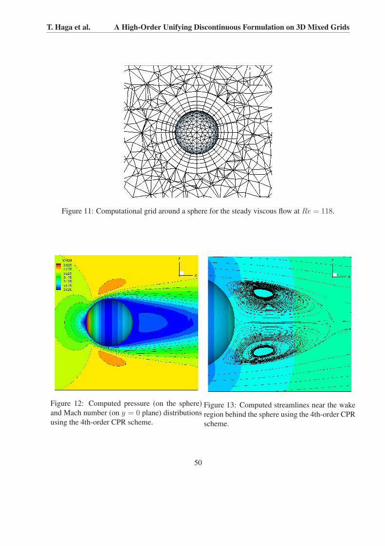
A steady viscous flow around a sphere is computed to validate the developed NS solver on a full3D mixed mesh. The Reynolds number based on the diameter was chosen to be 118 so that wecan compare the obtained results with experimental data [37] and numerical results using the SDscheme [36, 44]. The Mach number is 0.2535 that is the same value in the reference computations.The mesh is generated to have five layers of prism cells and isotropic tetrahedral cells for theremaining region. We plot the cut of the grid on a plane with y = 0 and surface mesh on the spherein Fig. 11. The total number of mixed cells is 24334.

The computations were performed using the 3rd- and 4th-order schemes. The computed Machnumber contours and streamlines near wake using the 4th-order CPR scheme are shown in Fig. 12and Fig. 13, respectively. We confirmed that the computed streamlines and the size of separationregion agree well with both the experimental picture and the numerical results in the references.Here we only show a comparison of the computed skin friction profiles at the cross section (y = 0)of the sphere in Fig. 14. The skin friction coefficients computed by the 4th-order CPR schemeand the 6th-order SD scheme are right on top of each other. The 3rd-order CPR result also agreeswell with other results, though one can see only minor differences between those profiles. Thepredicted separation angle using the 4th-order CPR scheme is 123.6 deg (the wind side stagnationpoint has an angle of 0), which is identical to the value predicted by the 6th-order SD scheme. InFig. 15, the computed drag coefficient by 4th-order CPR is compared to available experimentaldata. The agreement is also very good.

47


Figure 7: Comparisons of the skin friction coefficient along the plate.

Figure 8: Grid and Mach number contours ofa laminar boundary layer on a flat plate usingdegree k = 5 polynomial in the y-direction(stretched by a factor of 10 in y direction).

Figure 9: Comparison of v−velocity profiles us-ing different degrees of polynomial and grids.

48


(a) (b)

Figure 10: Comparisons of convergence histories using different degrees of polynomial and gridsin terms of time step and cpu time in (a) and (b).

5.2.4. Unteady Subsonic Flow over a Sphere at Re=300

We consider an unsteady flow case over the sphere with radius r = 1 at the Reynolds number of300 based on the diameter of the sphere. The inflow Mach number is assumed to be 0.3 in thiscase. The computational mesh is shown in Fig. 16. To resolve shedding vortices, the mesh isgenerated to have finer cells in the wake region. The total number of mixed cells is 54312. Localgrid size around the sphere is ∼ 0.2 and the size in the wake region is ∼ 0.8. In this case, weemployed the 3rd-order TVD Runge-Kutta method for the time integration and computed by theMPI parallelized code using 8 cores of a cluster machine to reduce the wall clock time.

The computed Q isosurface colored by local Mach number using the 4th-order CPR schemeis shown in Fig. 17. The obtained plain symmetric wake vortex structure is comparable to theavailable experimental and computational results in [10, 19] at least qualitatively. In Fig. 18 weplot the history of the drag coefficient Cd in terms of non-dimensional time t. The computed dragcoefficient and the oscillating amplitude of drag and the Strouhal number St are shown in Table4. For comparison, results from Gassner [10] using the 4th-order DG scheme on tetrahedral gridand from Tomboulides [38] and Johnson and Patel [19] obtained by incompressible simulation, areshown as well. The results computed by the CPR method reasonably agree with those referencevalues.

6. ConclusionsThe CPR method is successfully extended to 3D hybrid unstructured meshes using tetrahedral andprismatic elements. The CPR formulation for tetrahedral elements is directly derived in the same

49


Figure 11: Computational grid around a sphere for the steady viscous flow at Re = 118.

Figure 12: Computed pressure (on the sphere)and Mach number (on y = 0 plane) distributionsusing the 4th-order CPR scheme.

Figure 13: Computed streamlines near the wakeregion behind the sphere using the 4th-order CPRscheme.

50


-0.1

0

0.1

0.2

0.3

0.4

0 30 60 90 120 150 180

SD 6thCPR 3rdCPR 4th

CF

Figure 14: Comparison of computed skin fric-tion coefficients using the 3rd- and 4th order CPRschemes and 6th-order SD scheme in [44].

10-2

10-1

100

101

102

103

0.01 1 100 1e+4 1e+6

Exp.CPR 4th

CD

Re

Figure 15: Comparison between the computeddrag coefficient using the 4th-order CPR schemeand experimental data for a sphere.

Table 4: Comparisons of the averaged drag coefficient, the amplitude of drag and the Strouhalnumber.

Method Cd ΔCd StPresent 0.670 0.0032 0.131

Gassner [10] 0.673 0.0031 0.135Tomboulides [38] 0.671 0.0028 0.136

Johnson & Patel [19] 0.656 0.0035 0.137

manner as for 2D triangular elements and the one for prism is obtained by just a combination ofthe 1D and 2D schemes. The resulting scheme needs no explicit integrations and no data recon-structions. This numerical efficiency is more significant in 3D simulations in comparison to 2Dsimulations because numerical complexities involved in high-order quadratures and reconstruc-tions rapidly increase in 3D.

The developed CPR scheme is verified with grid convergence studies for an inviscid flow and aviscous flow, indicating that the developed scheme is capable of achieving nearly the optimal orderof accuracy. Then, several validation cases are computed for solving the 3D Euler equations andthe 3D NS equations. The CPR method performs very well to obtain high-order accurate solutionsfor all cases. Future studies include extension to adopt hexahedral and pyramidal cells for moreflexible geometry discretizations and hp-adaptation techniques for realizing practical high accurateCFD simulations.

51


(a) Entire grid (b) Grid around the sphere

Figure 16: Computational grid around a sphere for the unsteady viscous flow at Re = 300.

AcknowledgementsThis study has been supported by the Air Force Office of Scientific Research (AFOSR) undergrant FA9550-09-1-0128. The views and conclusions contained herein are those of the authors andshould not be interpreted as necessarily representing the official policies or endorsements, eitherexpressed or implied, of AFOSR.

References[1] F. Bassi, S. Rebay. A high-order accurate discontinuous finite element method for the nu-

merical solution of the compressible Navier-Stokes equations. J. Comput. Phys., 131 (1997),267–279.

[2] F. Bassi, S. Rebay. GMRES discontinuous Galerkin solution of the compressible Navier-Stokes equations. In B. Cockburn, G.E. Karniadakis, and C. W. Shu, editors, DiscontinuousGalerkin Methods: Theory, Computations and Applications, volume 11 of Lecture Note inComputational Science and Engineering. Springer, 2000.

[3] Q. Chen and I. Babuska. Approximate optimal points for polynomial interpolation of realfunctions in an interval and in a triangle. Comput. Methods Appl. Mech. Eng., 128 (1995),405-417.

52


Figure 17: Computed Q isosurfaces in the wakeregion of the viscous laminar flow over a sphereat Re = 300.

0.64

0.645

0.65

0.655

0.66

0.665

0.67

0.675

0.68

200 400 600 800 1000 1200 1400

CD

Time

Figure 18: Time history of the drag coefficientfor unsteady flow over a sphere at Re = 300.

[4] B. Cockburn, S. Y. Lin, C. W. Shu. TVD Runge-Kutta local projection discontinuous GalerkinFinite element method for conservation laws III: one-dimensional systems. J. Comput. Phys.,84 (1989), 90-113.

[5] B. Cockburn, C. W. Shu. TVD Runge-Kutta local projection discontinuous Galerkin Finiteelement method for conservation laws II: general framework. Math. Comput., 52 (1989) 411-435.

[6] B. Cockburn, C. W. Shu. The local discontinuous Galerkin method for time-dependentconvection-diffusion systems. SIAM J. Numer. Anal., 35 (1998), No. 6, 2440-2463.

[7] B. Cockburn, C. W. Shu. The Runge-Kutta discontinuous Galerkin method for conservationlaws V: multidimensional systems. J. Comput. Phys., 141 (1998), 199-224.

[8] K. Fidkowski, T. A. Oliver, J. Lu, D. Darmofal. p-Multigrid solution of high-order discontin-uous Galerkin discretizations of the compressible Navier-Stokes equations. J. Comput. Phys.,207 (2005), 92-113.

[9] H. Gao, Z. J. Wang. A high-order lifting collocation penalty formulation for the Navier-Stokes equations on 2D mixed grids. AIAA Paper 2009-3784, 2009.

[10] G. J. Gassner, F. Lorcher, C-D. Munz, and J. S. Hesthaven. Polymorphic nodal elements andtheir application in discontinuous Galerkin methods. J. Comput. Phys., 228 (2009), 1573-1590.

[11] S. K. Godunov. A difference scheme for numerical computation of discontinuous solutions ofequations of fluid dynamics. Math. Sbornik, 47 (1959), 271-306, In Russian.

53


[12] T. Haga, M. Furudate, K. Sawada. RANS simulation using high-order spectral volume methodon unstructured tetrahedral grids. AIAA Paper 2009–404, 2009.

[13] T. Haga, K. Sawada, Z. J. Wang. An implicit LU-SGS scheme for the spectral volume methodon unstructured tetrahedral grids. Communications in Computational Physics, 6 (2009),No.5, 978-996.

[14] R. Harris, Z. J. Wang, Y. Liu. Efficient quadrature-free high-order spectral volume methodon unstructured grids: Theory and 2D implementation. J. Comput. Phys., 227 (2008), 1620-1642.

[15] J. S. Hesthaven. From electrostatics to almost optimal nodal sets for polynomial interpolationin a simplex. SIAM J. Numer. Anal., 35 (1998), No.2, 655-676.

[16] H. T. Huynh. A flux reconstruction approach to high-order schemes including discontinuousGalerkin methods. AIAA Paper 2007–4079, 2007.

[17] H. T. Huynh. A reconstruction approach to high-order schemes including discontinuousGalerkin for diffusion. AIAA Paper 2009–403, 2009.

[18] A. Jameson. Analysis and design of numerical schemes for gas dynamics. I. Artificial diffu-sion, upwind biasing, limiters and their effect on accuracy and multigrid convergence. Int. J.Comput. Fluid Dyn., 4 (1994), 171–218.

[19] T. A. Johnson and V. C. Patel. Flow past a sphere up to a Reynolds number of 300. J. FluidMech., 378 (1999), 19-70.

[20] D. A. Kopriva and J. H. Kolias. A conservative staggered-grid Chebyshev multidomainmethod for compressible flows. J. Comput. Phys., 125 (1996), 244–261.

[21] M. S. Liou. A sequel to AUSM, Part II: AUSM+-up for all speeds. J. Comput. Phys., 214(2006), 137-170.

[22] Y. Liu, M. Vinokur, and Z. J. Wang. Discontinuous spectral difference method for conser-vation laws on unstructured grids. In Proceedings of the Third International Conference onComputational Fluid Dynamics, Toronto, Canada, July 2004.

[23] Y. Liu, M. Vinokur, and Z. J. Wang. Spectral difference method for unstructured grids I:Basic formulation. J. Comput. Phys., 216 (2006), 780-801.

[24] Y. Liu, M. Vinokur, Z. J. Wang. Spectral (finite) volume method for conservation laws onunstructured grids V: Extension to three-dimensional systems. J. Comput. Phys., 212 (2006),454-472.

[25] H. Luo, J. D. Baum, and R. Lohner. A discontinuous Galerkin method based on a Taylor basisfor the compressible flows on arbitrary grids. J. Comput. Phys., 227 (2008), 8875-8893.

54


[26] D. J. Mavriplis. Multigrid strategies for viscous flow solvers on anisotropic unstructuredmeshes. J. Comput. Phys., 145 (1998), 141-165.

[27] G. May, A. Jameson. A spectral difference method for the Euler and Navier-Stokes equations.AIAA Paper 2006–304, 2006.

[28] C. R. Nastase, D. J. Mavriplis. High-order discontinuous Galerkin methods using an hp-multigrid approach. J. Comput. Phys., 213 (2006), 330-357.

[29] S. Osher. Riemann solvers, the entropy condition, and difference approximations. SIAM J.Numer. Anal., 21 (1984), 217-235.

[30] W. H. Reed, T. R. Hill. Triangular mesh methods for the neutron transport equation. LosAlamos Scientific Laboratory Report LA-UR-73-479, 1973.

[31] P. L. Roe. Approximate Riemann solvers, parameter vectors, and difference schemes. J. Com-put. Phys., 43 (1981) 357-372.

[32] V. V. Rusanov. Calculation of interaction of non-steady shock waves with obstacles. J. Com-put. Math. Phys., 1 (1961), 267-279.

[33] S. J. Sherwin, G. E. Karniadaks. A new triangular and tetrahedral basis for high-order (hp)finite element methods. Int. J. Num. Meth. Eng., 38 (1995), 3775–3802.

[34] C. W. Shu. Total-variation-diminishing time discretizations. SIAM Journal on Scientific andStatistical Computing, 9 (1988), 1073-1084.

[35] C. W. Shu. Essentially non-oscillatory and weighted and non-oscillatory schemes for hyper-bolic conservation laws. In B. Cockburn, C. Johnson, C.-W. Shu, and E. Tadmor, editors,Advanced Numerical Approximation of Nonlinear Hyperbolic Equations, volume 1697 ofLecture Note in Mathematics. Springer, 1998.

[36] Y. Sun, Z. J. Wang, and Y. Liu. High-order multidomain spectral difference method for theNavier-Stokes equations on unstructured hexahedral grids. Communications in Computa-tional Physics, 2 (2007), 310-333.

[37] S. Taneda. Experimental investigations of the wake behind a sphere at low reynolds nombers.J. Phys. Soc. Japan, 11 (1956), 11041108.

[38] A. G. Tomboulides, S. A. Orzag. Numerical investigation of transitional and weak turbulentflow past a sphere. J. Fluid Mech., 416 (2000), 45-73.

[39] K. Van den Abeele and C. Lacor. An accuracy and stability study of the 2D spectral volumemethod. J. Comput. Phys., 226 (2007), 1007-1026.

[40] K. Van den Abeele, C. Lacor, Z. J. Wang. On the stability and accuracy of the spectraldifference method. J. Sci. Comput., 37 (2008), 162-188.

55


[41] B. Van Leer. Towards the ultimate conservative difference scheme V. A second order sequelto Godunovs method. J. Comput. Phys., 32 (1979), 110-136.

[42] B. Van Leer, S. Nomura. Discontinuous Galerkin for diffusion. AIAA Paper 2005–5108,2005.

[43] Z. J. Wang. Spectral (finite) volume method for conservation laws on unstructured grids:basic formulation. J. Comput. Phys., 178 (2002), 210-251.

[44] Z. J. Wang. High-order methods for the Euler and Navier-Stokes equations on unstructuredgrids. Progress in Aerospace Sciences, 43 (2007), 1-41.

[45] Z. J. Wang, H. Gao. A unifying lifting collocation penalty formulation including the discon-tinuous Galerkin, spectral volume/difference methods for conservation laws on mixed grids.J. Comput. Phys., 228 (2009), 8161-8186.

[46] Z. J. Wang, Y. Liu. Spectral (finite) volume method for conservation laws on unstructuredgrids II: Extension to two-dimensional scalar equation. J. Comput. Phys., 179 (2002) 665-697.

[47] Z. J. Wang, Y. Liu. Spectral (finite) volume method for conservation laws on unstructuredgrids III: One-dimensional systems and partition optimization. Journal of Scientific Comput-ing, 20 (2004), No.1, 137-157.

[48] Z. J. Wang, L. Zhang, Y. Liu. Spectral (finite) volume method for conservation laws on un-structured grids IV: Extension to two-dimensional systems. J. Comput. Phys., 194 (2004),716-741.

[49] T. Warburton. An explicit construction of interpolation nodes on the simplex. J. Eng. Math.,56 (2006), 247-262.

[50] O. C. Zienkiewicz, R. L. Taylor. The Finite Element Method The Basics, vol. 1. Butterworth-Heinemann, Oxford, England, 2000.

56

a high-order unifying discontinuous formulation for the

Documents