A High Resolution Daily Gridded Rainfall

Data for the Indian Region: Analysis of

break and active monsoon spells

M.Rajeevan, Jyoti Bhate, J.D.Kale

National Climate Centre India Meteorological Department

Pune, 411 005

B.Lal

India Meteorological Department New Delhi- 110 003

Address for correspondence Dr. M.Rajeevan National Climate Centre India Meteorological Department Pune- 411 005 INDIA rajeevan@imdpune.gov.in rajeevan61@yahoo.co.in

Abstract

In this paper, we report the development of a high resolution (10 X 10 Lat/Long)

gridded daily rainfall data set for the Indian region to fulfill the demands from the

research community. We have considered daily rainfall data of 6329 stations for the

interpolation analysis. However, there are only 1803 stations with a minimum 90%

data availability during the analysis period (1951-2003). We have used only those 1803

stations for interpolation in order to minimize the risk of generating temporal

inhomogeneities in the gridded data due to varying station densities. For the

analysis, we have followed the interpolation method proposed by Shepard (1968)

based on the weights calculated from the distance between the station and the grid

point and also the directional effects. Standard quality controls were performed before

carrying out the interpolation analysis.

Comparison with similar global gridded rainfall data sets revealed that the

present rainfall analysis is better in accurate representation of spatial rainfall variation.

The Global data sets underestimate the heavy rainfall along the west-coast and over

Northeast India. The inter-annual variability of southwest monsoon seasonal (June-

September) rainfall was found to be similar in all the data sets.

Using this gridded rainfall data set, an analysis was made to identify the break

and active periods during the southwest monsoon season (June to September). Break

(Active) periods during the monsoon season were identified as the periods in which the

standardized daily rainfall anomaly averaged over Central India (210- 270 N, 720 – 850

E) is less than -1.0 (more than 1.0). The break periods thus identified for the period

1951-2003 were found to be comparable with the periods identified by earlier studies. In

contrary to a recent study by Joseph and Simon (2005), no evidence was found for any

statistically significant trends in the number of break or active days during the period

1951-2003.

This gridded rainfall data set is available to the research community for non-

commercial applications.

1. Introduction

Information on spatial and temporal variations of rainfall is very important in

understanding the hydrological balance on a global/regional scale. The distribution of

precipitation is also important for water management for agriculture, power generation,

and drought monitoring. In India, rainfall received during the south-west monsoon

season (June to September) is very crucial for its economy. Real time monitoring of

rainfall distribution on daily basis is required to evaluate the progress and status of

monsoon and to initiate necessary action to control drought/flood situations.

High resolution observed rainfall data are also required to validate

regional/mesoscale models, and to examine and model the intra-seasonal oscillations

like Madden-Julian Oscillation (MJO) over the Indian region. Gridded rainfall data sets

are useful for regional studies on the hydrological cycle, climate variability and

evaluation of regional models. In the recent years, there has been a considerable

interest among different research groups in developing high resolution of gridded

rainfall data sets. (Huffman et al. 1997, Xie and Arkin 1997, Dai et a l. 1997, Rudolf et

al. 1998, Gruber et al.2000, New et al. 1999, Adler et al. 2003, Mitra et al. 2003, Chen

et al. 2004, Beck et al. 2005).

In this paper, we discuss the development of a high resolution (10 X 10

Latitude/Longitude) daily gridded rainfall data set for the Indian region for 53 years

(1951-2003). The details of data used, quality control adopted and the methodologies of

interpolation are discussed. 2. Rainfall Data and Quality Control

After the major drought of 1877 and the accompanying famine, India

Meteorological Department established a large network of rain gauge stations, which

provided a valuable source of data to analyze the space-time structure of the monsoon

rainfall and its variability. With the introduction of telegraph system, daily rainfall and

also other meteorological observations began to be collected and analysed on daily

basis. India Meteorological Department over the years has maintained very high

standards in monitoring the rainfall and other meteorological parameters over India with

great care and accuracy (Sikka 2003).

A brief historical account and description of the rainfall data collection by the IMD

are given by Walker (1910) and Parthasarathy and Mooley (1978). Using the IMD daily

rainfall data of 1901-1970, Hartman and Michelsen (1989) converted into a gridded

data set by grouping the station data into 10 Lat/Long grid boxes. Using this gridded

rainfall data set, Hartman and Michelsen (1989), Krishnamurthy and Shukla (2000) and

Krishnamurthy and Shukla (2005) studied the intra-seasonal and interannual variability

of rainfall over India.

For the present analysis, we have used the daily rainfall data archived at the

National Data Centre, India Meteorological Department (IMD), Pune. IMD operates

about 537 observatories, which measure and report rainfall occurred in the past 24

hours ending 0830 hours Indian Standard Time (0300 UTC). In addition, most of the

state governments also maintain rain-gauges, for real time rainfall monitoring. IMD

digitizes, quality controls and archives these data also along with rainfall data recorded

at IMD observatories. Before archiving, IMD makes multi-stage quality control of

observed values.

We have considered rainfall data for the period 1951-2003 for the present

analysis. Standard quality control is performed before carrying out the analysis. First,

station information (especially location) was verified, wherever the details are available.

The precipitation data themselves are checked for coding or typing errors. Many such

errors were identified, which were corrected by referring to the original manuscripts.

For the period, 1951-2003, IMD has the rainfall records of 6329 stations, with

varying periods. Out of these 6329 stations, 537 stations are the IMD observatory

stations, 522 stations are under the Hydrometeorology programme and 70 are Agromet

stations. Remaining stations are rainfall-reporting stations maintained by state

governments. However, only 1803 stations out of 6329 stations had a minimum 90%

data availability during the analysis period (1951-2003). We have used only those 1803

stations for which a minimum 90% data are available for the analysis in order to

minimize the risk of generating temporal inhomogeneities in the gridded data due to

varying station densities. The network of stations (1803 stations) considered for this

study is shown in Fig.1. The density of stations is not uniform throughout the country.

Density is the highest over south Peninsula and is very poor over northern plains of

India (Uttar Pradesh) and eastern parts of central India. Fig.2. shows the day to day

variation of number of rainfall stations, which were available for the analysis. On an

average 1600 station data were available for the analysis. However, during the recent

years, number of stations available for the analysis dropped significantly. This is due to

the delay in digitizing and archiving the manuscripts which are received at IMD in a

delayed mode.

3. Interpolation Method

There are different methods of numerical interpolation of irregularly distributed

data to a regular N-dimensional array (Thiebaux and Pedder (1987)). Bussieres and

Hogg (1989) studied the error of spatial interpolation using four different objective

methods. For application to the specific project grid, the statistical optimal interpolation

technique displayed the lowest root mean square errors. This technique and Shepard

OA, displayed zero bias and would be useful for areal average computations. The

GPCC used a variant of the spherical-coordinate adaptation of Shepard’s method

(Willmott et al. 1985) to interpolate the station data to regular grid points. These regular

points are then averaged to provide area mean, monthly total precipitation on 2.5 grid

cells. New et al. (1999) used the thin plate splines proposed by Hutchinson (1998).

Mitra et al (2003) used the successive correction method of Cressman (Krishnamurti et

al. 1983).

For the present analysis, we have used the interpolation scheme proposed by

Shepard (1968). In the Shepard (1968) method, interpolated values are computed from

a weighted sum of the observations. Given a grid point, the search distance is defined

as the distance from this point to a given station. The interpolation is restricted to the

radius of influence. For search distances equal to or greater than the radius of

influence, the grid point value is assigned a missing code when there is no station

location located within this distance. In this method, interpolation is limited to the radius

of influence. A predetermined maximum value limits the number of data points used

which, in the case of high data density, reduces the effective radius of influence. We

have also considered the method proposed by Shepard to locally modify the scheme

for including the directional effects and barriers. In this interpolation method, no initial

guess is required. More details of the method are given in Shepard (1968) and

Rajeevan et al. (2005).

We have interpolated station rainfall data into a rectangular grid of 35 X 32 grids

for each day for the period 1951-2003. The starting point of the grid is 6.50 N and 66.5 0

E. From this point, there are 35 points towards east and 32 points towards north. We

have created one binary file for each year. For the leap year, we have created data for

366 days.

4. Comparison with Global data set

After completing the rainfall analysis for the period 1951-2003, we have

compared the IMD gridded data set with VASClimo data set, which is a global gridded

rainfall data set. German Weather Service and Johann Wolfgang Goethe-University,

Frankfurt jointly carried out a climate research project, named Variability Analysis of

Surface Climate Observations (VASClimo), which was started in October 2001. Main

objective of this project is the creation of a new 50-year precipitation climatology for the

global land-areas gridded at three different resolutions (0.50 lat/lon, 10 lat/lon, and 2.5o

lat/lon) on the basis of quality controlled station data. More details of this new rainfall

climatology are available in Beck et al. (2005). To compare the IMD analysis with the

VASClimo data set, we have considered the VASClimo data of 1951-2000. Since both

these global data are available on monthly time scale, we have added IMD daily

gridded rainfall data into monthly total before comparing with the global data sets. The

results of comparison of the southwest monsoon seasonal (June to September) rainfall

only are presented here.

Fig.3. shows the spatial distribution of the seasonal (June-September) mean

rainfall averaged for the period 1951-2003 derived from the IMD gridded rainfall data

set. The rainfall pattern suggests maximum along the west coast of India and NE India.

Rainfall minimum is observed over NW India as well as over SE India.

Fig.4.a shows the difference between the present analysis (IMD) and VASClimo

data set and Fig 4.b shows the correlation coefficient between the IMD analysis and

VASClimo data set.

Over the most parts of India, the differences between the VASClimo data and

IMD data are of the order of 50mm only. However, along the west coast of India, IMD

rainfall values are more than the VASClimo values. However, the correlations between

VASClimo and IMD rainfall data are very large (exceeding even 0.6) over central and

NW parts of India. Over Gujarat and central Peninsula, correlations exceed even 0.8.

We have further compared the inter-annual variations of rainfall among the data

set. For this purpose, area weighted rainfall for the southwest monsoon (June-

September) season was calculated with all the two data sets. However, we have

excluded NE parts of India for calculating the area weighted rainfall. The seasonal

mean and standard deviation of rainfall of two data sets are given below:

Rainfall Product

Mean Rainfall Coefficient of variation

IMD

(1951-2003)

836.3 mm

11.6 %

VASClimo

(1951-2000)

844.0 mm

12.1%

The two data set shows similar coefficient of variation, i.e.12%. Fig. 5 shows the

interannual variation of southwest monsoon seasonal (June-September) rainfall

calculated from IMD analysis as well as VASClimo data set. There is an excellent

similarity in the inter-annual rainfall variation among the different data sets with all major

drought and excess years were well captured the two data sets. The correlation

coefficient between the IMD and VASClimo data sets is 0.95 (for the period 1951-

2000).

5. Analysis of Break Days

The gridded daily rainfall data, presented in this report will be useful for many

applications. Some of the possible applications are validation of general circulation and

numerical weather prediction models and studies on intra-seasonal variability like active

and break cycles. In the past, similar gridded data sets (1901-1970) were used to

examine the intra-seasonal variability (Hartmann and Michelsen 1989, Krishnamurthy

and Shukla, 2003, Krishnamurthy and Shukla 2005) of the Indian summer monsoon.

The present rainfall data set has been used to identify the active–break periods

during the southwest monsoon season. Long intense breaks are often associated with

poor monsoon seasons, and they have a large impact on rainfed agriculture (Gadgil

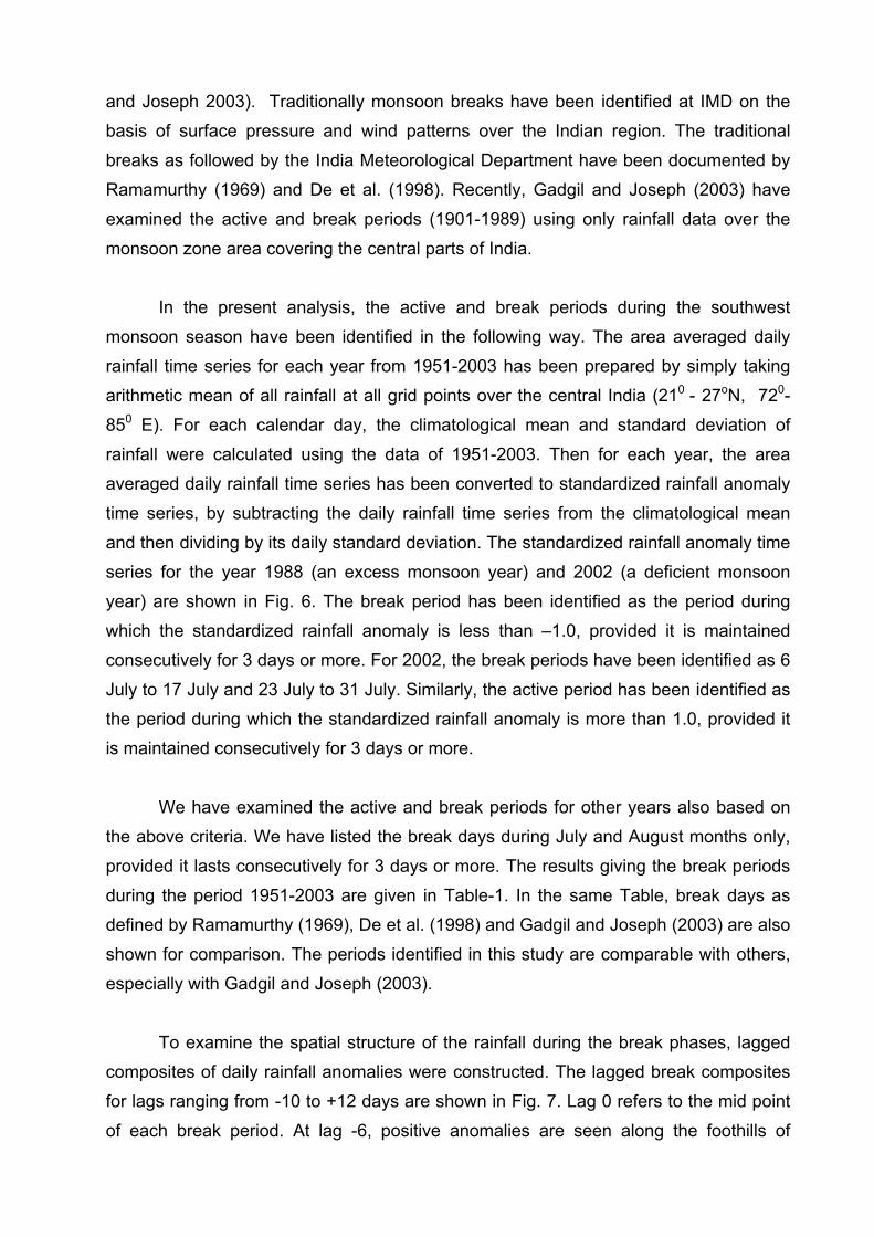
and Joseph 2003). Traditionally monsoon breaks have been identified at IMD on the

basis of surface pressure and wind patterns over the Indian region. The traditional

breaks as followed by the India Meteorological Department have been documented by

Ramamurthy (1969) and De et al. (1998). Recently, Gadgil and Joseph (2003) have

examined the active and break periods (1901-1989) using only rainfall data over the

monsoon zone area covering the central parts of India.

In the present analysis, the active and break periods during the southwest

monsoon season have been identified in the following way. The area averaged daily

rainfall time series for each year from 1951-2003 has been prepared by simply taking

arithmetic mean of all rainfall at all grid points over the central India (210 - 27oN, 720-

850 E). For each calendar day, the climatological mean and standard deviation of

rainfall were calculated using the data of 1951-2003. Then for each year, the area

averaged daily rainfall time series has been converted to standardized rainfall anomaly

time series, by subtracting the daily rainfall time series from the climatological mean

and then dividing by its daily standard deviation. The standardized rainfall anomaly time

series for the year 1988 (an excess monsoon year) and 2002 (a deficient monsoon

year) are shown in Fig. 6. The break period has been identified as the period during

which the standardized rainfall anomaly is less than –1.0, provided it is maintained

consecutively for 3 days or more. For 2002, the break periods have been identified as 6

July to 17 July and 23 July to 31 July. Similarly, the active period has been identified as

the period during which the standardized rainfall anomaly is more than 1.0, provided it

is maintained consecutively for 3 days or more.

We have examined the active and break periods for other years also based on

the above criteria. We have listed the break days during July and August months only,

provided it lasts consecutively for 3 days or more. The results giving the break periods

during the period 1951-2003 are given in Table-1. In the same Table, break days as

defined by Ramamurthy (1969), De et al. (1998) and Gadgil and Joseph (2003) are also

shown for comparison. The periods identified in this study are comparable with others,

especially with Gadgil and Joseph (2003).

To examine the spatial structure of the rainfall during the break phases, lagged

composites of daily rainfall anomalies were constructed. The lagged break composites

for lags ranging from -10 to +12 days are shown in Fig. 7. Lag 0 refers to the mid point

of each break period. At lag -6, positive anomalies are seen along the foothills of

Himalayas, associated with the shift of the monsoon trough over that region. At lag -10

days, negative rainfall anomalies appear over east central parts of India, which increase

and slowly expand northwestwards. At lag 0, large negative anomalies cover most parts

of India except NE and SE parts of India. Positive anomalies over SE parts of India first

develop around lag -8 and slowly expand in area. From lag +2 days, negative

anomalies over central parts of India decrease both in area and magnitude. During this

period, positive anomalies slowly move northwest wards. By Lag +12, large positive

anomalies are seen along the west coast. With the revival of monsoon, at lag +12,

positive anomalies appear over the coast of Orissa and adjoining area.

Recently, Joseph and Simon (2005) reported that duration of break (weak)

monsoon spells in a monsoon season has increased by 30% during the period 1950-

2002. Number of days with daily average rainfall less than 8mm/day (break or weak

monsoon spells) increased and number of days with daily average rainfall more than 12

mm/day (active monsoon spells) decreased during the same period. These are alarm

findings for a country whose food production and economy depend heavily on monsoon

rainfall.

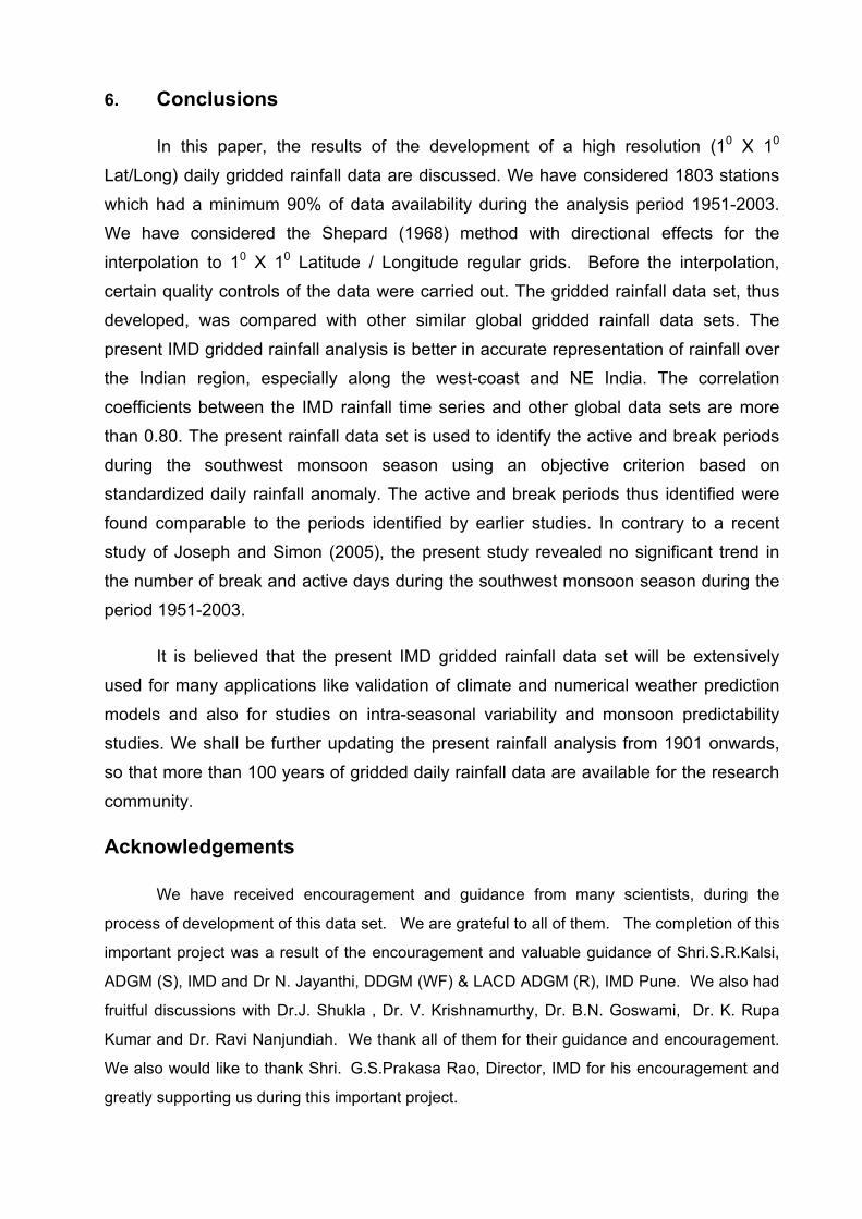
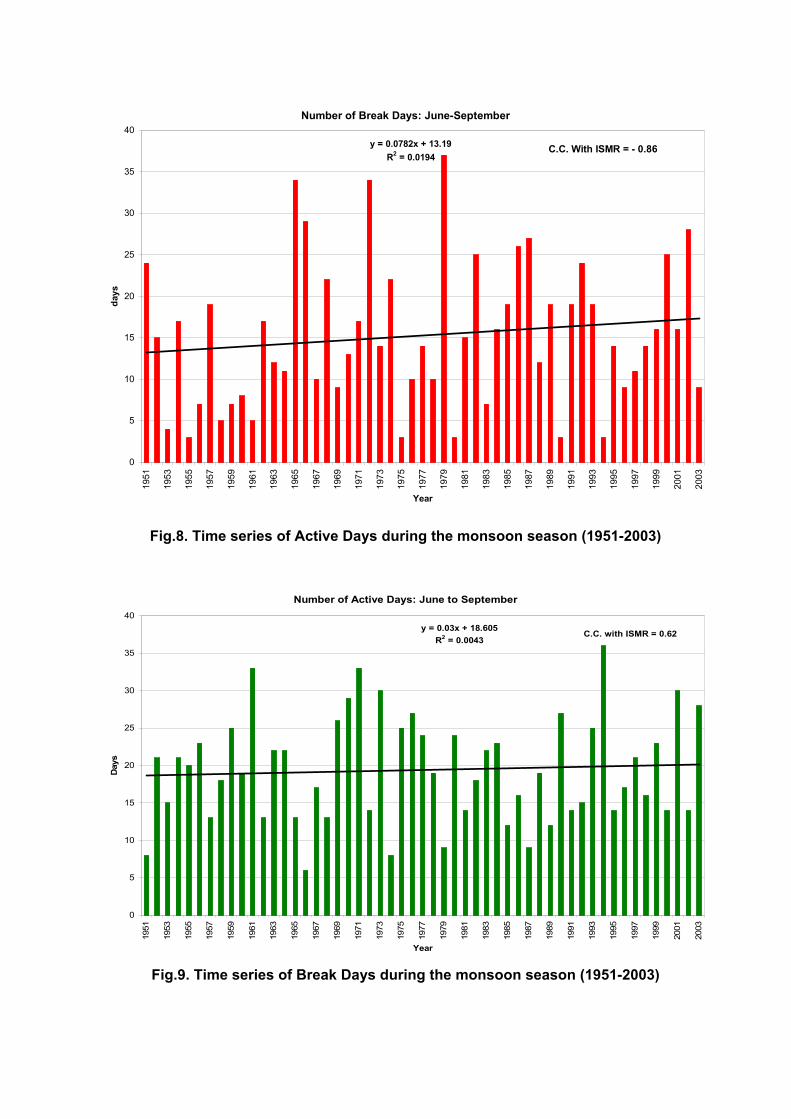
To confirm the findings of Joseph and Simon (2005) and to further explore the

issue, we have made an analysis with 53 years of IMD daily gridded rainfall data. Using

the standardized daily rainfall anomaly averaged over the Central India (210 – 270 N,

720 to 850 E), number break and active days during the period June to September were

calculated for each year for the period 1951-2003. The time series of number of break

and active days for the period 1951-2003 are shown in Fig. 8 and 9 respectively. The

time series of break days has a very high negative correlation (-0.86) with southwest

monsoon seasonal (June to September) rainfall. With the time series of active days, the

corresponding correlation is +0.62. In the study of Joseph and Simon (2005), the

number of break and active days were identified using a different criterion as mentioned

in the above paragraph for the period 1950-2002. Their study revealed weaker

correlations of -0.58 and 0.54 respectively for number of break and active days. Thus

the time series of break and active days prepared in this study is a more representative

measure of monsoon activity during the season. However, Figs. 8 and 9 do not show

any statistically significant trend either in number of break days or number of active

days, which is in contrary from the results of Joseph and Simon (2005).

6. Conclusions

In this paper, the results of the development of a high resolution (10 X 10

Lat/Long) daily gridded rainfall data are discussed. We have considered 1803 stations

which had a minimum 90% of data availability during the analysis period 1951-2003.

We have considered the Shepard (1968) method with directional effects for the

interpolation to 10 X 10 Latitude / Longitude regular grids. Before the interpolation,

certain quality controls of the data were carried out. The gridded rainfall data set, thus

developed, was compared with other similar global gridded rainfall data sets. The

present IMD gridded rainfall analysis is better in accurate representation of rainfall over

the Indian region, especially along the west-coast and NE India. The correlation

coefficients between the IMD rainfall time series and other global data sets are more

than 0.80. The present rainfall data set is used to identify the active and break periods

during the southwest monsoon season using an objective criterion based on

standardized daily rainfall anomaly. The active and break periods thus identified were

found comparable to the periods identified by earlier studies. In contrary to a recent

study of Joseph and Simon (2005), the present study revealed no significant trend in

the number of break and active days during the southwest monsoon season during the

period 1951-2003.

It is believed that the present IMD gridded rainfall data set will be extensively

used for many applications like validation of climate and numerical weather prediction

models and also for studies on intra-seasonal variability and monsoon predictability

studies. We shall be further updating the present rainfall analysis from 1901 onwards,

so that more than 100 years of gridded daily rainfall data are available for the research

community.

Acknowledgements

We have received encouragement and guidance from many scientists, during the

process of development of this data set. We are grateful to all of them. The completion of this

important project was a result of the encouragement and valuable guidance of Shri.S.R.Kalsi,

ADGM (S), IMD and Dr N. Jayanthi, DDGM (WF) & LACD ADGM (R), IMD Pune. We also had

fruitful discussions with Dr.J. Shukla , Dr. V. Krishnamurthy, Dr. B.N. Goswami, Dr. K. Rupa

Kumar and Dr. Ravi Nanjundiah. We thank all of them for their guidance and encouragement.

We also would like to thank Shri._G.S.Prakasa Rao, Director, IMD for his encouragement and

greatly supporting us during this important project.

References

Adler, R.F., Huffman, G.J., and Coauthors, 2003, The version-2 Global Precipitation

Climatology Project (GPCC) Monthly precipitation analysis (1979-present),

J.Hydrometeorology, 4, 1147-1167.

Beck,C., Grieser, J., and Rudolf, B., 2005, A New monthly precipitation climatology for the

Global Land Areas for the Period 1951-2000, Climate Status Report 2004, German

Weather Service, Offenbach, Germany, 10 pp.

Bussieres, N and W.Hogg, 1989, The Objective analysis of daily rainfall by distance weighting

schemes on a mesoscle grid, Atmosphere-Ocean, 3, 521-541.

Chen, M., P.Xie, J.E.Janowiak, and P.A.Arkin, 2002, Global Land Precipitation: A 50 yr monthly

Analysis Based on Gauge Observations, J.Hydrometeorology, 3, 249-266.

Dai, A., Fung, I., and Genio, D.G., 1997, Surface observed global land precipitation variations

during 1900-1998, J.Climate, 10, 2943-2962.

De, U.S., Lele,R.R., and Natu, J.C., 1998, Breaks in southwest monsoon, India Meteorological

Department, Report no 1998/3.

Gadgil, S., and Joseph, P.V., 2003, On breaks of the Indian monsoon, Proc.Indian.Acad.Sci.

(Earth and Planet Sci), 112, 4, 529-558.

Gruber, A., X Su, M.Kanamitsu, and J.Schemm, 2000, The comparison of two merged rain

gauge –satellite precipitation data sets, Bull.Amer.Met.Soc., 81, 2631-2644.

Hartman, D.L., and M.L.Michelsen, 1989, Intraseasonal periodicities in Indian rainfall,

J.Atmos.Sci., 46, 2838-2862.

Huffman, G.J., and Coauthors, 1997, The Global Precipitation Climatology Project (GPCC)

combined precipitation data sets, Bull.Amer.Meteor.Soc., 78, 5-20.

Hutchinson, M.F,1998, Interpolation of rainfall data with thin plate smoothing splines: I two

dimensional smoothing of data with short range correlation. Journal of Geographic

Information and Decision Analysis 2(2): 152-167

Joseph, P.V., and Anu Simon, 2005, Weakening trend of the southwest monsoon current

through peninsular India from 1950 to the present, Current Science, 89, 4, 687-694.

Krishnamurti, T.N., S.Cocke, R.Pasch, and S.Low-Nam, 1983, Precipitation estimates from rain

gauge and satellite observations, summer MONEX, FSU report 83-7, Department of

Meteorology, The Florida State University, 373 pp.

Krishnamurthy, V., and J.Shukla, 2000, Intra-seasonal and Inter-annual variability of rainfall

over India, J.Climate, 13, 4366-4377.

Krishnamurthy, V., and J.Shukla, 2005, Intraseasonal and seasonally persisting patterns of

Indian monsoon rainfall, COLA Technical Report, CTR 188, June 2005, pp41.

Mitra, A.K., M.Das Gupta, S.V.Singh and T.N.Krishnamurti, 2003, Daily rainfall for the Indian

monsoon region from merged satellite and raingauge values: Large scale analysis from

real time data, J.Hyrdrometeorology, 4, 769-781.

New, M, Hulme, M. and Jones, P.D., 1999, Representing Twentieth-Century Space-Time

Variability. Part I: Development of a 1961-1990 Mean Monthly Terrestrial Climatology,

J.Climate, 1999, 12, 829-856.

Parthasarathy, B., and Mooley,D.A., Some features of a long homogenous series of Indian

summer monsoon rainfall, Mon.Wea.Rev., 106, 771-781.

Rajeevan, M., Jyoti Bhate, J.D.Kale and B.Lal, 2005, Development of a high resolution daily

gridded rainfall data for the Indian region, IMD Met Monograph No: Climatology

22/2005, pp27. (Available from National Climate Centre, IMD Pune.

ncc@imdpune.gov.in).

Ramamurthy, K., 1969, Monsoon of India: Some aspects of the “ Break” in the Indian southwest

monsoon during July and August, Forecasting Manual, 1-57, No. IV, 18.3, India

Met.Dept, Poona, India.

Rudolf, B., H.Hauschild, W.Ruth, and U.Schneider, 1994, Terrestrial precipitation analysis:

Operational method and required density of point measurements, Global Precipitation

and Climate Change, M.Desbois and E.Desalmand, Eds NATO ASI Series I, Vol.26,

Springer-Verlag, 173-186.

Shepard, D., 1968, A two-dimensional interpolation function for irregularly spaced data, Proc.

1968 ACM Nat.Conf, pp 517-524.

Sikka, D.R., 2003, Evaluation of monitoring and forecasting of summer monsoon over India and

a review of monsoon drought of 2002, Proc.Indian Natn.Sci.Acad. 69, 5, 479-504.

Theibaux, H.J., and Pedder, M.A., 1987, Spatial Objective analysis with Applications in

Atmospheric Science, Academic Press, London.

Walker, G.T., 1910, On the meteorological evidence for supposed changes of climate in India,

Indian. Meteor.Memo, 21, Part –I, 1-21.

Willmott, C.J., C.M.Rowe, and W.D.Philpot, 1985, Small-scale climate maps: A sensitivity

analysis of some common assumptions associated with grid-point interpolation and

contouring, Amer.Cartographer, 12, 5-16.

Xie, P., and P.A.Arkin, 1997, Global Precipitation: A 17-year monthly analysis based on gauge

observations, satellite measurements and numerical models outputs,

Bull.Amer.Meteor.Soc., 78, 2539-2558.

Table-1 Break days identified in the present analysis and previous studies

YEAR BREAK DAYS – JULY & AUGUST (1951-1989)

Gadgil and Joseph (2003)

Ramamurthy (1969) up to 1967

De et al. (2002) from 1968 to 1989

Present analysis

1951 14-15J, 24-30A 1-3 J, 11-13 J, 15-17 J,

24-29A

9-14J, 21-24J,

25-30A

1952 1-3 J, 10-13J, 27-30A 9-12J 9-15J

1953 - 24-26J -

1954 22-29A 18-29J, 21-25A 22-29A

1955 24-25J 22-29J -

1956 23-30A 23-26A 23-30A

1957 28-29J 27-31J, 5-7A -

1958 - 10-14A -

1959 - 16-18A -

1960 20-24J, 30-31A 16-21J 20-23J

1961 - - -

1962 27-28J, 1-2A, 7-8A, 25-26A 18-22A 27-29A

1963 18-19J, 22-23J 10-13J, 17-21J 16-18J, 21-23J

1964 - 14-18J, 28J-3A 1-5 A

1965 7-11J, 4-14A 6-8J, 4-15A 6-14J, 3-14A, 17-19 A

1966 2-12J, 22-31A 2-11J, 23-27A 2-13J, 24-31A

1967 6-15J 7-10J 10-14J

1968 25-31A 25-29A 25-31A

1969 27-31A 17-20A, 25-27A 29-31A

1970 14-19J, 23-26J 12-25J 14-19J, 23-26J

1971 8-10J, 5-6A, 18-19A 17-20A 5-7 A, 18-20 A

1972 19J-3A 17J-3A 11-14J, 19J-3A

1973 24-26J, 30J-1A 23J-1A 24- 26 J

1974 24-26A, 29-31A 30-31A 29-31 A

1975 - 24-28J -

1976 3-4J, 21-22A - 1-4 J

1977 15-19A 15-18A 14-21A

1978 - 16-21J -

1979 2-6J, 15-31A 17-23J, 15-31A 2-7J, 12-31A

1980 17-20J, 14-15A 17-20J -

1981 19-20A, 24-31A 26-30J, 23-27A 26-31 A

1982 1-8J - 1-9J , 16-19 J

1983 8-9J, 24-26A 22-25A 7-9J , 14-16 J

1984 - 20-24J 12-14 A

1985 2-3J, 23-25A 22-25A 11-13 A, 24-27A

1986 1-4J, 31J-2A, 22-31A 23-26A, 29-31A 3-5 J, 26-31A

1987

16-17J, 23-24J, 31J-4A,

11-13A 28J-1A

16-18 J, 30 J- 3A,

8-10A, 14-18A

1988 14-17A 5-8J, 13-15A 15-17A

1989 30-31J 10-12J, 29-31J 18-20J, 31J- 3A

YEAR

BREAK DAYS (1990-2003)

Present Analysis

1990 -

1991 2-8J

1992 4-10J

1993 19-23J, 8-14A

1994 -

1995 4-7 J

1996 3-5 J

1997 13-17A

1998 21-26J

1999

1-5 J , 18-20 A,

22-24 A

2000

22-24 J, 2-8A,

24-27A

2001 -

2002 5-16J, 22 J- 31 J

2003 -

Fig.1. Locations of 1803 Rain gauge stations

NO. OF STATIONS PER DAY (1951-2003)(for stations with >=40 yrs of data)

0

200

400

600

800

1000

1200

1400

1600

1800

2000

1951

1953

1955

1957

1959

1961

1963

1965

1967

1969

1971

1973

1975

1977

1979

1981

1983

1985

1987

1989

1991

1993

1995

1997

1999

2001

2003

YEAR

NO

. OF

STA

TIO

NS

Fig.2. Number of stations per day available for the analysis

Fig. 3. Spatial pattern of southwest monsoon seasonal (June to September) mean rainfall

Fig.4.a. The difference (in mm) between the IMD gridded rainfall data and VASClimo

gridded rainfall data for the southwest monsoon season. Period: 1951-2000

Fig.4.b. Correlation Coefficient between the IMD rainfall data and VASClimo rainfall data during the southwest monsoon season

(June-September). Period of analysis: 1951-2000.

COMPARISON OF IMD DATA FOR ALL INDIA ZONAL AVG. FOR JUNE-SEPTWITH VASCLIM ZONAL AVG (1951-2000)

60

70

80

90

100

110

120

130

140

1951

1953

1955

1957

1959

1961

1963

1965

1967

1969

1971

1973

1975

1977

1979

1981

1983

1985

1987

1989

1991

1993

1995

1997

1999

2001

YEAR

% O

F LP

A

IMD DATAVASCLIM

Fig. 5. Interannual variation of southwest monsoon season (June- September) rainfall

from the IMD gridded analysis and VASClimo analysis. Period: 1951-2003

Fig.6. The standardized rainfall anomaly time series for the year a) 1988 and b) 2002 for the period 1 June to 30 September.

STANDARDISED ANOMALY FOR DAILY RAINFALL : 1988

-3.0

-2.0

-1.0

0.0

1.0

2.0

3.0

1-Ju

n

8-Ju

n

15-J

un

22-J

un

29-J

un

6-Ju

l

13-J

ul

20-J

ul

27-J

ul

3-A

ug

10-A

ug

17-A

ug

24-A

ug

31-A

ug

7-S

ep

14-S

ep

21-S

ep

28-S

ep

DATE

STD

. AN

OM

ALY

STANDARDISED ANOMALY FOR DAILY RAINFALL : 2002

-3.0

-2.0

-1.0

0.0

1.0

2.0

3.0

4.0

1-Ju

n

8-Ju

n

15-J

un

22-J

un

29-J

un

6-Ju

l

13-J

ul

20-J

ul

27-J

ul

3-A

ug

10-A

ug

17-A

ug

24-A

ug

31-A

ug

7-S

ep

14-S

ep

21-S

ep

28-S

ep

DATE

STD

. AN

OM

ALY

Lag (-2) Lag (0) Lag (+2) Lag (+4) Lag (+6) Lag (+8) Lag (+10) Lag (+12)

Fig.7. Lagged Break phase composites of daily rainfall anomalies (mm/ day) for June-Sept season 1951-2003. Lag 0 corresponds to the mid point of each break phase.

Number of Break Days: June-September

y = 0.0782x + 13.19R2 = 0.0194

0

5

10

15

20

25

30

35

40

1951

1953

1955

1957

1959

1961

1963

1965

1967

1969

1971

1973

1975

1977

1979

1981

1983

1985

1987

1989

1991

1993

1995

1997

1999

2001

2003

Year

days

C.C. With ISMR = - 0.86

Fig.8. Time series of Active Days during the monsoon season (1951-2003)

Number of Active Days: June to September

y = 0.03x + 18.605R2 = 0.0043

0

5

10

15

20

25

30

35

40

1951

1953

1955

1957

1959

1961

1963

1965

1967

1969

1971

1973

1975

1977

1979

1981

1983

1985

1987

1989

1991

1993

1995

1997

1999

2001

2003

Year

Day

s

C.C. with ISMR = 0.62

Fig.9. Time series of Break Days during the monsoon season (1951-2003)