a high-resolution mapped grid algorithm for compressible

Journal of Computational Physics 229 (2010) 8780–8801

Contents lists available at ScienceDirect

Journal of Computational Physics

journal homepage: www.elsevier .com/locate / jcp

A high-resolution mapped grid algorithm for compressible multiphaseflow problems

K.-M. Shyue *

Department of Mathematics, National Taiwan University, Taipei 106, Taiwan

a r t i c l e i n f o

Article history:Received 3 May 2010Received in revised form 16 July 2010Accepted 8 August 2010Available online 18 August 2010

Keywords:Compressible multiphase flowFluid-mixture modelMapped gridsWave-propagation methodStiffened gas equation of state

0021-9991/$ - see front matter � 2010 Elsevier Incdoi:10.1016/j.jcp.2010.08.010

* Tel.: +886 2 3366 2866; fax: +886 2 2391 4439.E-mail address: [email protected]

a b s t r a c t

We describe a simple mapped-grid approach for the efficient numerical simulation of com-pressible multiphase flow in general multi-dimensional geometries. The algorithm uses acurvilinear coordinate formulation of the equations that is derived for the Euler equationswith the stiffened gas equation of state to ensure the correct fluid mixing when approxi-mating the equations numerically with material interfaces. A c-based and a a-based modelhave been described that is an easy extension of the Cartesian coordinates counterpartdevised previously by the author [30]. A standard high-resolution mapped grid methodin wave-propagation form is employed to solve the proposed multiphase models, givingthe natural generalization of the previous one from single-phase to multiphase flow prob-lems. We validate our algorithm by performing numerical tests in two and three dimen-sions that show second order accurate results for smooth flow problems and also free ofspurious oscillations in the pressure for problems with interfaces. This includes also sometests where our quadrilateral-grid results in two dimensions are in direct comparisonswith those obtained using a wave-propagation based Cartesian grid embedded boundarymethod.

� 2010 Elsevier Inc. All rights reserved.

1. Introduction

Our goal is to describe a simple mapped-grid approach for efficient numerical resolution of compressible multiphase flowin general multi-dimensional geometries. As a first endeavor towards the method development, we are concerned with asimplified model problem, where the flow regime of interest is assumed to be homogeneous with no jumps in the pressureand velocity (the normal component of it) across the material interface separating two regions of different fluid componentswithin a spatial domain. In this problem, the physical effects such as the viscosity, surface tension, and heat conduction areassumed to be small, and hence can be ignored. With that, we use an Eulerian viewpoint of the governing equations that theprincipal motion of each fluid component in a Cartesian coordinates can be written as

@

@t

qqui

E

0B@1CAþXNd

j¼1

@

@xj

quj

quiuj þ pdij

Euj þ puj

0B@1CA ¼ 0 ð1Þ

for i ¼ 1;2; . . . ;Nd. Here Nd denotes the number of spatial dimensions. The quantities q,uj,p,E, and dij are the density, particlevelocity in the xj-direction, pressure, total energy, and the Kronecker delta, respectively.

. All rights reserved.

http://dx.doi.org/10.1016/j.jcp.2010.08.010

mailto:[email protected]

http://dx.doi.org/10.1016/j.jcp.2010.08.010

http://www.sciencedirect.com/science/journal/00219991

http://www.elsevier.com/locate/jcp

K.-M. Shyue / Journal of Computational Physics 229 (2010) 8780–8801 8781

To close the model, for simplicity, the constitutive law for each fluid phase is assumed to satisfy a linearized Mie-Grün-eisen (i.e., the linearly density-dependent stiffened gas) equation of state of the form

pðq; eÞ ¼ ðc� 1Þqeþ ðq� q0ÞB ð2Þ
for approximating materials including compressible liquids and solids (cf. [14,25]). Here e represents the specific internalenergy. The quantities c,q0, and B are the ratio of specific heats (c > 1), the reference values of density, and speed of soundsquared, respectively. We have E ¼ qeþ
PNdj¼1qu2

j =2 as usual.In this work, we want to generalize a state-of-the-art shock-capturing method that was devised originally for single-phase

flows on mapped grids to the case of a multiphase flow. It is well known that the principal problem in the usual extension is theoccurrence of spurious pressure oscillations when two or more fluid components are present in a grid cell (cf. [5] and referencestherein). Here the algorithm uses a curvilinear coordinate formulation of a fluid-mixture model that is composed of the Eulerequations of gas dynamics for the basic conserved variables and an additional set of effective equations for the problem-depen-dent material quantities. In this approach, as in its Cartesian coordinates counterpart (cf. [30,31]), the latter equations are de-rived to ensure the correct fluid mixing when approximating the equations numerically with material interfaces, see Section 2.With the proposed model equations, accurate results can be obtained on a mapped grid using a standard method, such as thehigh-resolution wave- propagation algorithm for a single-phase flow (cf. [8,9,21]), see Section 4 for numerical examples.

There are quite a few other numerical approaches available in the literature for approximating compressible multiphaseproblems over a multi-dimensional domain with complex geometries. Some representative ones are the overlapping gridmethod [5], the unstructured grid methods [2,11,43], and the Cartesian grid embedded boundary method [35].

An advantage of the mapped-grid approach described here is that extension of the method from two to three dimensions canbe done in a straightforward manner for simple geometries such as cylinders, spheres, and their variants [9]. This is in contrastwith the extension of an unstructured or a Cartesian grid method, where it requires a significant algorithmic and programmingeffort to realize each of the methods that are designed of general purpose. In addition to that, if we want to use a front trackingmethod to improve numerical resolution of shock waves and interfaces, with complex geometries involved, it would be relativelyeasier to apply the method on a body-fitted mapped grid than on a fixed Cartesian grid, see [17,37] for an example. Furthermore,it is also easy to combine the method with a class of moving mesh techniques (cf. [38,40]) for efficient solution adaptation.

It should be mentioned that the methodology we have given here is by no means limited to the current case with thestiffened gas equation of state. Extension of the method to problems involving more complicated equations of state canbe made by considering, for instance, either a c-based model of the author [32] or a a-based model of Allaire et al. [3](see Section 2.2), and proceeding with the idea described in this paper. Without going into the details for that, our goal isto establish the basic solution strategy and validate its use via some sample numerical experimentations; this is a necessarystep for our further development of the method towards more complicated problems of fundamental importance(cf. [15,18,27,28] and references therein).

The format of this paper is as follows: in Section 2, we describe our mathematical model for a simplified homogeneousmultiphase flow in curvilinear coordinates. In Section 3, we review briefly the wave-propagation method on mapped grids.Numerical results of some sample test problems in two and three dimensions are presented in Section 4.

2. Mathematical models in curvilinear coordinates

The basic governing equations in our mapped grid algorithm consist of two parts. We use the Euler equations in a curvilinearcoordinate as a model system for the motion of the fluid mixtures of the conserved variables in a multiphase grid cell. With that,from the mass and energy conservations, we derive a set of effective equations for the problem-dependent material quantitiesin those cells, see below, that can be used directly to the determination of the pressure from the equation of state. Combiningthis two set of the equations together with the equation of state constitutes a complete mathematical model that is fundamen-tal in our mapped grid algorithm for numerical approximation of multiphase flow problems with complex geometries.

To find out the aforementioned equations in a three-dimensional Nd = 3 curvilinear coordinate system, for example, weintroduce a coordinate mapping from the physical domain (x1,x2,x3) to the computational domain (n1,n2,n3) via the relations

dx1 ¼ a1dn1 þ a2dn2 þ a3dn3;

dx2 ¼ b1dn1 þ b2dn2 þ b3dn3;

dx3 ¼ c1dn1 þ c2dn2 þ c3dn3;

ð3Þ

where ai,bi,ci for i ¼ 1; 2; 3 are the metric terms of the mapping. Then under this mapping, the Euler equation (1) can betransformed into the new coordinate system as

@q@tþ 1

J

XNd

j¼1

@

@njðqUjÞ ¼ 0;

@

@tðquiÞ þ

1J

XNd

j¼1

@

@njðquiUj þ pJjiÞ ¼ 0; i ¼ 1;2; . . . ;Nd;

@E@tþ 1

J

XNd

j¼1

@

@njðEUj þ pUjÞ ¼ 0;

ð4Þ

8782 K.-M. Shyue / Journal of Computational Physics 229 (2010) 8780–8801

where Uj ¼PNd

i¼1uiJji is the contravariant velocity in the nj-direction for j = 1,2, . . . ,Nd. Here the quantities Jij for i, j = 1,2,3 areas a consequence of the coordinate transformation that satisfies the following expressions:

J11 J12 J13

J21 J22 J23

J31 J32 J33

0B@1CA ¼ b2c3 � b3c2 a3c2 � a2c3 a2b3 � a3b2

b3c1 � b1c3 a1c3 � a3c1 a3b1 � a1b3

b1c2 � b2c1 a2c1 � a1c2 a1b2 � a2b1

0B@1CA ð5Þ

and the quantity J = detj@(x1,x2,x3)/@(n1,n2,n3)j is the Jacobian of the mapping which can be computed by

J ¼X3

i¼1

aiJ1i ¼X3

i¼1

biJ2i ¼X3

i¼1

ciJ3i: ð6Þ

Note that during the initialization step, all the coordinate transformation variables such as ai,bi,ci, J1i, J2i, J3i for i = 1,2,3, and Jwould be determined and remained fixed at all time when a mapped grid is constructed by a chosen numerical grid gener-ator (cf. [9,39]).

It is easy to see that (3) would be a two-dimensional coordinate mapping from (x1,x2) to (n1,n2) for any spatial location x3

in the physical domain, if we have a simplified data set where the quantities a3,b3,c1, and c2 are all zero, and c3 is equal toone. In this instance, if we set Nd = 2 in (4) with the coordinate transformation variables defined as in (5) and (6), we wouldhave the same Euler equations in a two-dimensional curvilinear coordinate when a mapping of the form

dx1 ¼ a1dn1 þ a2dn2;

dx2 ¼ b1dn1 þ b2dn2;ð7Þ

is used in the derivation (cf. [4,7,16,42]). Thus, without causing any confusion, we may simply use the symbol Nd as in theCartesian case, see (1), to represent the number of spatial dimension in the curvilinear coordinate formulation of equations.

2.1. c-based model equations

To derive the effective equations for the mixture of material quantities in curvilinear coordinates, one approach is to startwith an interface-only problem (cf. [30,32–34]) where both the pressure and each phase of the particle velocities are con-stant in the domain, while the other variables such as the density and the material quantities are having jumps across someinterfaces. Then, from (4), it is easy to obtain an equation for the time-dependent behavior of the total internal energy as

@

@tðqeÞ þ 1

J

XNd

j¼1

Uj@

@njðqeÞ ¼ 0:

Now, by inserting (2) into the above equation, we find an alternative form:

@

@tp

c� 1� q� q0

c� 1B

� �þ 1

J

XNd

j¼1

Uj@

@nj

pc� 1

� q� q0

c� 1B

� �¼ 0; ð8Þ

that is in relation to not only the pressure, but also the density and the material quantities c,q0, and B.In our algorithm, to maintain the pressure in equilibrium as it should be for this interface-only problem and also to deter-

mine all the three material quantities in (2), we split (8) into the following three equations for the fluid mixture of1=ðc� 1Þ;qB=ðc� 1Þ, and q0B=ðc� 1Þ as

@

@t1

c� 1

� �þ 1

J

XNd

j¼1

Uj@

@nj

1c� 1

� �¼ 0; ð9Þ

@

@tqB

c� 1

� �þ 1

J

XNd

j¼1

Uj@

@nj

qBc� 1

� �¼ 0; ð10Þ

@

@tq0Bc� 1

� �þ 1

J

XNd

j¼1

Uj@

@nj

q0Bc� 1

� �¼ 0; ð11Þ

respectively. As before (cf. [31–34]), since in practice we are interested in shock wave problems as well, we should take theequations, i.e., (9)–(11), in a form so that all the three material quantities remain unchanged across both shocks and rare-faction waves. In this regard, it is easy to see that with 1/(c � 1) and q0B=ðc� 1Þ governed in turn by (9) and (11), thereis no problem to do so (cf. [1,30]). For qB=ðc� 1Þ, however, due to the dependence of the density term, it turns out that,in a time when such a situation occurs, for consistent with the mass conservation law of the fluid mixture in (4), the prim-itive form of (10) should be modified by

@

@tqB

c� 1

� �þ 1

J

XNd

j¼1

@

@nj

qBc� 1

Uj

� �¼ 0; ð12Þ


so that the mass-conserving property of the solution in the single-phase region can be acquired also.In summary, combining the Euler equation (4) and the set of effective equations: (9), (11), and (12), yields a so-called c-

based model system as

@q@tþ 1

J

XNd

j¼1

@

@njðqUjÞ ¼ 0;

@

@tðquiÞ þ

1J

XNd

j¼1

@

@njðquiUj þ pJjiÞ ¼ 0; i ¼ 1;2; . . . ;Nd;

@E@tþ 1

J

XNd

j¼1

@


@

@t1

c� 1

� �þ 1

J

XNd

j¼1

Uj@

@nj

1c� 1

� �¼ 0;

@

@tq0Bc� 1

� �þ 1

J

XNd

j¼1

Uj@

@nj

q0Bc� 1

� �¼ 0;

@

@tqB

c� 1

� �þ 1

J

XNd

j¼1

@

@nj

qBc� 1

Uj

� �¼ 0;

ð13Þ

this gives us Nd + 5 equations to be solved in total that is nicely independent of the number of fluid phases involved in theproblem. With a system expressed in this way, there is no problem to compute all the state variables of interests, includingthe pressure from the equation of state

p ¼ E�PNd

i¼1ðquiÞ2

2qþ qB

c� 1

� �� q0B

c� 1

� �" #,1

c� 1

� �: ð14Þ

For the ease of the latter discussion, it is useful to write (13) into a more compact expression by

@q@tþ 1

J

XNd

j¼1

@

@njfjðqÞ þ BjðqÞ

@q@nj

� �¼ 0; ð15Þ

with

q ¼ q;qu1; . . . ;quNd; E;

1c� 1

;q0Bc� 1

;qB

c� 1

� �T

;

fj ¼ qUj;qu1Uj þ pJj1; . . . ;quNdUj þ pJj;Nd

; EUj þ pUj;0;0;qB

c� 1Uj

� �T

;

Bj ¼ diagð0;0; . . . ;0; 0;Uj;Uj;0Þ;

ð16Þ

for j ¼ 1;2; . . . ;Nd. Note that in the Cartesian coordinates case where the coordinate mapping quantities a1,b2,c3 are all equalto one, while the remaining ones are all zeros, Eq. (15) reduces to

@q@tþXNd

j¼1

@

@xj

�f jðqÞ þ �BjðqÞ@q@xj

� �¼ 0; ð17Þ

with �f j and �Bj defined in turn by

�f j ¼ quj;qu1uj þ pd1j; . . . ;quNduj þ pd3j; Euj þ puj;0;0;

qBc� 1

uj

� �T

;

�Bj ¼ diagð0;0; . . . ;0; 0;uj;uj;0Þ:ð18Þ

Then it is easy to check that fj and Bj are related to �f j and �Bj via

fj ¼XNd

i¼1

�f iJji and Bj ¼XNd

i¼1

�BiJji;

respectively.


With these notations, by assuming the proper smoothness of the solutions, the quasi-linear form of our model (15) can bewritten as

@q@tþ 1

J

XNd

j¼1

ðAjðqÞ þ BjðqÞÞ@q@nj¼ 0; ð19Þ

where Aj ¼ @fj=@q ¼PNd

i¼1�AiJji is the Jacobian matrix of fj with �Ai ¼ @�f i=@q for i ¼ 1;2; . . . ;Nd. If we assume further that the

thermodynamic description of the materials of interest is limited by the stability requirement, it is a straightforward matterto show that any linear combination of the matrices �Ai þ �Bi for i ¼ 1;2; . . . ;Nd is diagonalizable with real eigenvalues and acomplete set of linearly independent right eigenvectors (cf. [33]). Hence, we may conclude that our multiphase model ishyperbolic. Regarding discontinuous solutions of the system, such as shock waves or contact discontinuities, we find theusual form of the Rankine–Hugoniot jump conditions across the waves (cf. [13]).

2.2. a-based model equations

Before proceeding further, it should be mentioned that to define the initial fluid mixtures 1=ðc� 1Þ;qB=ðc� 1Þ, andq0B=ðc� 1Þ in a grid cell that contains Mf P 1 different fluid phases where each of them occupies a distinct region with avolume-fraction function ai 2 [0,1] in relation to it for i ¼ 1;2; . . . ;Mf ;

PMf

i¼1ai ¼ 1, we use the equation of state (2) of the form

qe ¼XMf

i¼1

aiqiei ¼XMf

i¼1

aipi

ci � 1�

qi � q0;i

ci � 1Bi

� �¼ p

c� 1� q� q0

c� 1B:

Here the subscript ‘‘i” denotes the state variable of fluid phase i. By taking a similar approach as employed in Section 2.1 forthe derivation of the c-based effective equations it comes out readily a splitting of the above expression into the relations:

1c� 1

¼XMf

i¼1

ai

ci � 1;

qBc� 1

¼XMf

i¼1

aiqiBi

ci � 1;

q0Bc� 1

¼XMf

i¼1

aiq0;iBi

ci � 1; ð20Þ

where in the process of splitting the terms we have imposed the condition

pc� 1

¼XMf

i¼1

aipi

ci � 1: ð21Þ

Clearly when each of the partial pressures is in an equilibrium state within a grid cell, in conjunction with the first part of(20), the pressure p obtained from (21) would remain in the same equilibrium as well, i.e., p = pi for i ¼ 1;2; . . . ;Mf .

Now if the above volume-fraction notion of the states 1=ðc� 1Þ;qB=ðc� 1Þ, and q0B=ðc� 1Þ are being employed in the c-based effective equations together with the usual definition of the mixture density q ¼

PMf

i¼1aiqi, we are able to rewrite themstraightforwardly into a componentwise form as

@

@tai

ci � 1

� �þ 1

J

XNd

j¼1

Uj@

@nj

ai

ci � 1

� �¼ 0; ð22Þ

@

@taiqiBi

ci � 1

� �þ 1

J

XNd

j¼1

@

@nj

aiqiBi

ci � 1Uj

� �¼ 0; ð23Þ

@

@taiq0;iBi

ci � 1

� �þ 1

J

XNd

j¼1

Uj@

@nj

aiq0;iBi

ci � 1

� �¼ 0; ð24Þ

i ¼ 1;2; . . . ;Mf . Then based on the fact that all the material quantities ci;Bi, and q0,i will be kept as a constant in each phase ofthe domain at all time, from (22) or (24), it is easy to find the transport equation for the volume-fraction ai as

@ai

@tþ 1

J

XNd

j¼1

Uj@ai

@nj¼ 0; ð25Þ

whereas, from (23), we find the conservation law for the phasic density aiqi as

@

@tðaiqiÞ þ

1J

XNd

j¼1

@

@njðaiqiUjÞ ¼ 0: ð26Þ

It is apparent that, if the solutions of ai and aiqi are known from the equations for i ¼ 1;2; . . . ;Mf , we may, therefore, com-pute 1/(c � 1), qB=ðc� 1Þ, and q0B=ðc� 1Þ directly according to (20). Thus, instead of using the c-based effective equations,it is a viable alternate to use the a-based equations: (25) and (26), for the motion of the mixture of the material quantities ofthe problem.


To sum up, combining (25) and (26) with the momentum and energy equations in (4) yields a a-based (or called volume-fraction) model system that can be written as

@

@tðaiqiÞ þ

1J

XNd

j¼1

@

@njðaiqiUjÞ ¼ 0; i ¼ 1;2; . . . ;Mf ;

@

@tðquiÞ þ

1J

XNd

j¼1

@

@njquiUj þ pJji

� �¼ 0; i ¼ 1;2; . . . ;Nd;

@E@tþ 1

J

XNd

j¼1

@


@ai

@tþ 1

J

XNd

j¼1

Uj@ai

@nj¼ 0; i ¼ 1;2; . . . ;Mf � 1;

ð27Þ

this gives us totally 2Mf + Nd equations to be solved. Here analogously to (14) the pressure can be determined from the equa-tion of state

p ¼ E�PNd

i¼1ðquiÞ2

2qþXMf

i¼1

aiqiBi

ci � 1�XMf

i¼1

aiq0;iBi

ci � 1

" #,XMf

i¼1

ai

ci � 1;

where we have assumed aMf¼ 1�

PMf�1i¼1 ai.

It is clear that (27) can be written of the form (15) in which we have q, fj, and Bj defined by

q ¼ a1q1; . . . ;aMfqMf

;qu1; . . . ;quNd; E;a1; . . . ;aMf�1

� �T;

fj ¼ a1q1Uj; . . . ;aMfqMf

Uj;qu1Uj þ pJj1; . . . ;quNdUj þ pJj;Nd

; EUj þ pUj;0; . . . ;0� �T

;

Bj ¼ diagð0; . . . ;0; . . . ;0;Uj; . . . ;UjÞ:

In a similar manner, in the Cartesian coordinates case where the system is of the form (17), we have �f j and �Bj defined by

�f j ¼ a1q1uj; . . . ;aMfqMf

uj;qu1uj þ pdj1; . . . ;quNduj þ pdj;Nd

; Euj þ puj;0; . . . ;0� �T

;

�Bj ¼ diagð0; . . . ;0; . . . ;0;uj; . . . ;ujÞ:

We note that since the derivation of the a-based model follows closely to the c-based model, it can be shown that this modelis hyperbolic also (cf. [3] for the Cartesian coordinates case) and is as effective as the c-based model for multiphase flowproblems with the stiffened gas equation of state. But for problems with Mf P 3, the c-based model is a prefer one touse, because the basic equations for the model stay as Nd + 5, see (13), irrespective of the number of fluid phases involvedin the problem.

2.3. Include source terms

To end this section, we comment that if x1 is the axisymmetric direction, an axisymmetric version of our multiphase mod-els in two dimensions can be written as

@q@tþ 1

J

X2

j¼1

@

@njfjðqÞ þ BjðqÞ

@q@nj

� �¼ wðqÞ; ð28Þ

where w is the source term derived directly from the geometric simplification. That is, we find

w ¼ � 1x1

qu1;qu21;qu1u2; Eu1 þ pu1;0;0;

qBc� 1

u1

� �T

; ð29Þ

when the c-based model is considered, and have

w ¼ � 1x1

a1q1u1; . . . ;aMfqMf

uMf;qu2

1;qu1u2; Eu1 þ pu1;0; . . . ;0� �T

;

when the a-based model is considered. In addition to that, if gravity is the only body force in the problem formulation, in thec-based model, for example, we may add in the following source term:

w ¼ �ð0;0;qg;qgu2;0; 0;0ÞT

as well. Here g denotes the gravitational constant. As to the other source terms such as the one arise from the surface tensionforce at the interface, we may use a continuum surface force model of Brackbill et al. [6] for that, see the work done by Peri-


gaud and Saurel [26] and the references therein for more details. Since it is beyond the scope of this paper, we will not dis-cuss this further.

3. Numerical approximation on mapped grids

We use a state-of-the-art finite volume method in wave-propagation form (cf. [9,21]) for the numerical discretization ofour multiphase flow models (without the source terms) on mapped grids. The method is based on solving one-dimensionalRiemann problems at each cell edge, and the waves (i.e., discontinuities moving at constant speeds) arising from the Rie-mann problem are employed to update the cell averages in the cells neighboring each edge.

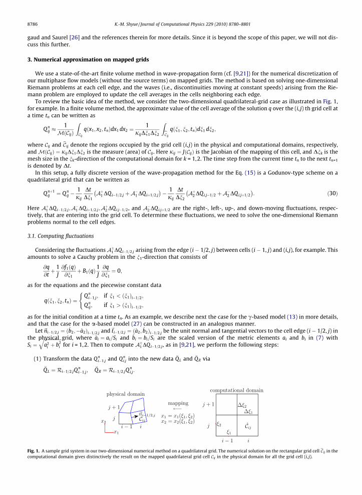
To review the basic idea of the method, we consider the two-dimensional quadrilateral-grid case as illustrated in Fig. 1,for example. In a finite volume method, the approximate value of the cell average of the solution q over the (i, j) th grid cell ata time tn can be written as

Fig. 1.comput

Qnij �

1MðCijÞ

ZCij

qðx1; x2; tnÞdx1 dx2 ¼1

jijDn1Dn2

ZbC ij

qðn1; n2; tnÞdn1 dn2;

where Cij and bC ij denote the regions occupied by the grid cell (i, j) in the physical and computational domains, respectively,andMðCijÞ ¼ jijDn1Dn2 is the measure (area) of Cij. Here jij ¼ JðCijÞ is the Jacobian of the mapping of this cell, and Dnk is themesh size in the nk-direction of the computational domain for k = 1,2. The time step from the current time tn to the next tn+1

is denoted by Dt.In this setup, a fully discrete version of the wave-propagation method for the Eq. (15) is a Godunov-type scheme on a

quadrilateral grid that can be written as

Qnþ1ij ¼ Q n

ij �1jij

DtDn1

Aþ1 DQ i�1=2;j þA�1 DQ iþ1=2;j

� �� 1

jij

DtDn2

Aþ2 DQ i;j�1=2 þA�2 DQi;jþ1=2

� �: ð30Þ

Here Aþ1 DQ i�1=2;j;A�1 DQiþ1=2;j;Aþ2 DQ i;j�1=2, and A�2 DQ i;jþ1=2 are the right-, left-, up-, and down-moving fluctuations, respec-tively, that are entering into the grid cell. To determine these fluctuations, we need to solve the one-dimensional Riemannproblems normal to the cell edges.

3.1. Computing fluctuations

Considering the fluctuationsA�1 DQ i�1=2;j arising from the edge (i � 1/2, j) between cells (i � 1, j) and (i, j), for example. Thisamounts to solve a Cauchy problem in the n1-direction that consists of

@q@tþ 1

J@f1ðqÞ@n1

þ B1ðqÞ1J@q@n1¼ 0;

as for the equations and the piecewise constant data

qðn1; n2; tnÞ ¼Q n

i�1;j; if n1 < ðn1Þi�1=2;

Q nij; if n1 > ðn1Þi�1=2;

(
as for the initial condition at a time tn. As an example, we describe next the case for the c-based model (13) in more details,and that the case for the a-based model (27) can be constructed in an analogous manner.
Let~ni�1=2;j ¼ ðb2;�a2Þi�1=2;j and~ti�1=2;j ¼ ða2; b2Þi�1=2;j be the unit normal and tangential vectors to the cell edge (i � 1/2, j) inthe physical grid, where ai ¼ ai=Si and bi ¼ bi=Si are the scaled version of the metric elements ai and bi in (7) withSi ¼

ffiffiffiffiffiffiffiffiffiffiffiffiffiffiffiffia2

i þ b2i

qfor i = 1,2. Then to compute A�1 DQ i�1=2;j, as in [9,21], we perform the following steps:

(1) Transform the data Q ni�1;j and Qn

i;j into the new data �QL and �QR via

�QL ¼ Ri�1=2;jQni�1;j;

�Q R ¼ Ri�1=2;jQni;j:

A sample grid system in our two-dimensional numerical method on a quadrilateral grid. The numerical solution on the rectangular grid cell bC ij in theational domain gives distinctively the result on the mapped quadrilateral grid cell Cij in the physical domain for all the grid cell (i, j).


Here Ri�1=2;j is a rotation matrix defined by

Ri�1=2;j ¼

1 0 0 00 ðb2Þi�1=2;j �ða2Þi�1=2;j 0

0 ða2Þi�1=2;j ðb2Þi�1=2;j 00 0 0 I

0BBB@1CCCA

with I in it as being a 4 � 4 identity matrix. Clearly this rotation matrix rotates the velocity components of Q into componentsnormal and tangential to the cell edge, and leaves the remaining components unchanged.

(2) Solve Riemann problem in the ‘‘x1” direction for

@q@tþ @

@x1

�f 1ðqÞ þ �B1ðqÞ@q@x1¼ 0 ð31Þ

with �f 1 and �B1 defined by (18) and the Riemann data �QL and �Q R.When an approximate Riemann solver is used for the numerical resolution, this would result in three propagating discon-tinuities that are moving with speeds �k1;k

i�1=2;j and the jumps �W1;ki�1=2;j across each of them for k = 1,2,3, see [31,33,34] for an

example.(3) Define scaled speeds

k1;ki�1=2;j ¼ ðS2Þi�1=2;j

�k1;ki�1=2;j

and rotate jumps back to the Cartesian coordinates by

W1;ki�1=2;j ¼ R

Ti�1=2;j

�W1;ki�1=2;j

for k = 1,2,3.(4) Determine the left- and right-moving fluctuations in the form

A�1 DQ i�1=2;j ¼X3

k¼1

k1;ki�1=2;j

� ��W1;k

i�1=2;j:

As usual, the notations for the quantities k± are set by k+ = max(k,0) and k� = min(k,0).

In a similar manner, we may determine the up- and down-moving fluctuations at the edge (i, j � 1/2) in the form

A�2 DQ i;j�1=2 ¼X3

k¼1

k2;ki;j�1=2

� ��W2;k

i;j�1=2

that is as the result of solving

@q@tþ 1

J@f2ðqÞ@n2

þ B2ðqÞ1J@q@n2¼ 0

with the initial data Qni;j�1 and Q n

i;j.

3.2. High-resolution corrections

To achieve high-resolution (i.e., second order accurate on smooth solutions, and sharp and monotone profiles on discon-tinuous solutions), the speeds and the limited version of the jumps are used to construct the piecewise linear correctionterms as before (cf. [21]), and are added to (30) in flux difference form as

Q nþ1ij : Q nþ1

ij � 1jij

DtDn1

eF 1iþ1=2;j � eF 1

i�1=2;j

� �� 1

jij

DtDn2

eF 2i;jþ1=2 � eF 2

i;j�1=2

� �:

Here at the edge (i � 1/2, j) the correction flux takes the form

eF i�1=2;j ¼12

X3

k¼1

k1;ki�1=2;j

1� Dtji�1=2;jDn1

k1;ki�1=2;j

� �fW1;ki�1=2;j;

and analogously at the edge (i, j � 1/2) the correction flux has the form

eF 2i;j�1=2 ¼

12

X3

k¼1

k2;ki;j�1=2

1� Dtji;j�1=2Dn2

k2;ki;j�1=2

� �fW2;ki;j�1=2;

where ji�1/2,j = (ji�1,j + ji,j)/2 and ji,j�1/2 = (ji,j�1 + ji,j)/2. The quantity fWm;k is a limited value ofWm;k obtained by comparingWm;k with the correspondingWm;k from the neighboring Riemann problem to the left (if km,k > 0) or to the right (if km,k < 0) form = 1,2 and k = 1,2,3.


In addition to that, a transverse propagation of wave is also included in the method as a part of the high-resolution cor-rection terms. Here the right-moving fluctuation Aþ1 DQ i�1=2;j, for instance, is decomposed into transverse fluctuationsA�2A

þ1 DQi�1=2;j which can be used to update the solutions above and below cell (i, j). In a similar manner, the left-moving fluc-

tuation A�1 DQi�1=2;j is split into A�2A�1 DQi�1=2;j which are used to update the solutions above and below cell (i � 1, j), see [21]

for the details.With the transverse wave-propagation, the method is typically stable as long as the time step Dt satisfies a variant of the

CFL (Courant–Friedrichs–Lewy) condition of the form

m ¼ Dt maxi;j;k

k1;ki�1=2;j

jip ;jDn1

;k2;k

i;j�1=2

ji;jp Dn2

0@ 1A 6 1; ð32Þ

where ip = i if k1;ki�1=2;j > 0 and i � 1 if k1;k

i�1=2;j < 0; jp is defined analogously (cf. [40]). Furthermore, by following the basic stepsdiscussed in [9,21], it can be shown that the method is quasi-conservative in the sense that when applying the method to ourmultiphase model (15) not only the conservation laws but also the transport equations are approximated in a consistentmanner by the method.

3.3. Three-dimensional extension

To extend this mapped grid method from two to three space dimensions, we use hexahedral meshes in place of quadri-lateral-grid cells, see Fig. 11 for an example. We use the fluctuation form of the method as usual in three dimensions for thesolution updates that is an easy generalization of the three-dimensional wave-propagation method on Cartesian grids pro-posed by Langseth and LeVeque [19] and also the two-dimensional method on mapped grid [21]. To implement the method,it is useful to make reference to the CLAWPACK webpage, see [9,36] in particular, for the programming details. In Section 4.2,we present some sample results that show the feasibility of this method to practical compressible multiphase problems.

4. Numerical results

We now present numerical results to validate our mapped grid algorithm for compressible multiphase flow problems intwo and three dimensions. Note that in this section we have only present solutions obtained using the c-based model (13) tothe method. This is because we have found a little difference between the results as compared to the ones using the a-basedmodel (27) to the method for simulations.

4.1. Two-dimensional case

4.1.1. Smooth vortex flowWe begin our tests by performing a convergence study of the computed solutions for a two-dimensional vortex evolution

problem (cf. [12,29,43]) that shows the order of accuracy that is attained for our high-resolution method as the mesh is re-fined. In this problem, we assume a single-phase ideal gas flow with c = 1.4 and B ¼ 0 in the stiffened gas equation of state(2). Initially, over a square domain of size [0,10] � [0,10], the state variables for the vortex are set by

q ¼ 1� ðc� 1Þ�2

8cp2 expð1� r2Þ� �1=ðc�1Þ

;

p ¼ qc;

u1 ¼ 1� �2p

expðð1� r2Þ=2Þ x2 � �x2ð Þ;

u2 ¼ 1þ �2p

expðð1� r2Þ=2Þðx1 � �x1Þ;

where r ¼ffiffiffiffiffiffiffiffiffiffiffiffiffiffiffiffiffiffiffiffiffiffiffiffiffiffiffiffiffiffiffiffiffiffiffiffiffiffiffiffiffiffiffiffiffiffiffiðx1 � �x1Þ2 þ ðx2 � �x2Þ2

qis the distance between points (x1,x2) and the vortex center ð�x1; �x2Þ ¼ ð5;5Þ, and � = 5 is

the vortex strength. Note that the above states are as the results of an isentropic perturbation in p/q,u1, and u2 to the meanflow with �q ¼ 1; �p ¼ 1; �u1 ¼ 1, and �u2 ¼ 1, and it is known that with the periodic conditions in both the x1- and x2-directionthe exact solution for this problem is simply the passive motion of a smooth vortex by the mean flow velocity.

We compare the behavior of the high-resolution wave-propagation method described in Section 3 on three differenttypes of grids as illustrated in Fig. 2:

Grid 1: Cartesian grids with square grid cells.Grid 2: Quadrilateral grids of the type described in [10].Grid 3: Quadrilateral grids of the type described in [9].

see [22] for a similar computation on the transport of a scalar quantity in a divergence-free velocity field. In order to estimatethe order of accuracy of the method, for each grid type, we compute the solution at the mesh refinement sequence:

0 5 100

2

4

6

8

10

0 5 100

2

4

6

8

10

0 5 100

2

4

6

8

10

Fig. 2. Three types of grids used for the smooth vortex flow problem.

Table 1High-resolution results for the smooth vortex test on Grid 1; one- and maximum-norm errors in primitive variables are shown.

N E1ðqÞ Order E1ðu1Þ Order E1ðu2Þ Order E1ðpÞ Order

40 0.6673 2.3443 1.7121 0.814380 0.1792 1.90 0.6194 1.92 0.4378 1.97 0.2128 1.94

160 0.0451 1.99 0.1537 2.01 0.1104 1.99 0.0536 1.99320 0.0113 2.00 0.0384 2.00 0.0276 2.00 0.0134 2.00

N EmðqÞ Order Emðu1Þ Order Emðu2Þ Order EmðpÞ Order

40 0.1373 0.3929 0.1810 0.174280 0.0377 1.87 0.1014 1.95 0.0502 1.85 0.0482 1.85

160 0.0093 2.02 0.0248 2.03 0.0123 2.03 0.0119 2.02320 0.0022 2.07 0.0062 2.00 0.0030 2.04 0.0029 2.04



40 0.9298 2.6248 2.1119 1.210480 0.2643 1.81 0.7258 1.85 0.5296 2.00 0.3277 1.89

160 0.0674 1.97 0.1833 1.99 0.1309 2.02 0.0845 1.96320 0.0169 2.00 0.0458 2.00 0.0327 2.00 0.0212 1.99


40 0.1676 0.4112 0.2259 0.211180 0.0471 1.83 0.1242 1.73 0.0645 1.79 0.0586 1.85

160 0.0126 1.91 0.0333 1.90 0.0162 2.02 0.0149 1.97320 0.0033 1.93 0.0085 1.97 0.0040 2.00 0.0038 1.98


DnðiÞ1 ¼ DnðiÞ2 ¼ DnðiÞ ¼ 1=2ðiþ2Þ for i = 0,1,2,3, i.e., by using an N � N grid for N = 40,80,160 and 320. To ensure that our conver-gence study is not adversely affected by a loss of accuracy near local extrema in the solution, there is no limiter being used inthe computations. In addition, the Courant number m = 0.9 defined by (32), and the Roe approximate Riemann solver areemployed in the tests.

Numerical results at time t = 10 obtained from all the 12 tests are presented in Tables 1–3. Here E1ðzÞ and EmðzÞ denote inturn the sequence of the one- and maximum-norm error of the cell-average solution in z to the true solution at the cell centerfor z = q,u1,u2, and p. We estimate the rate of convergence using the errors on two consecutive grids based on the formula

convergence order ¼ lnEði�1Þ

k ðzÞEðiÞk ðzÞ

!,ln

Dnði�1Þ

DnðiÞ

!
for k = 1,m and i = 1,2,3.
From the tables, we observe that the method is second order accurate in most cases on this problem. It is important tonote that the error behavior of the method on Grid 2 is on the same order of magnitude on Grid 1, the Cartesian grid, whilethis is not the case on Grid 3 which is a less smooth grid as compared to Grid 2. This indicates that the use of a smooth grid ina mapped grid method can indeed give a better resolution of the solution.



40 4.8272 4.7734 5.3367 5.471780 1.5740 1.62 1.5633 1.61 1.5660 1.77 1.5634 1.81

160 0.4536 1.79 0.4559 1.78 0.4537 1.79 0.4560 1.78320 0.1215 1.90 0.1221 1.90 0.1222 1.89 0.1221 1.90


40 0.4481 0.4475 0.4765 0.481780 0.1170 1.94 0.1181 1.92 0.1196 1.99 0.1191 2.02

160 0.0434 1.43 0.0431 1.45 0.0442 1.43 0.0440 1.44320 0.0117 1.89 0.0119 1.86 0.0119 1.89 0.0118 1.89

Fig. 3. Numerical results for an interface-only problem in a quarter annulus at time t = 520 ls. On the top, surface plots of the density and pressure areshown, and on the bottom, cross-sectional plot (along the line n2 = p/4) of the density and scatter plots of the relative error of the pressure are displayed,respectively. Here the solid line is the exact solution, and the dashed line is the initial condition at the time t = 0.


4.1.2. Passive interface evolutionWe are next concerned with an interface-only problem that the exact solution consists of a circular water column evolv-

ing in the air with uniform equilibrium pressure �p ¼ 105 Pa and constant particle velocity (�u1; �u2Þ = (103,103) m/s throughouta quarter annulus domain. Here we take the initial condition that inside the column of radius r0 = 0.2 m about the centerð�x1; �x2Þ ¼ ð0:8;0:8Þm the fluid is water with the data

ðq; c;q0;BÞr6r0¼ ð103 kg=m3

;4:4;103 kg=m3;2:64� 106 ðm=sÞ2Þ;

while outside the column the fluid is air with the data

ðq; c;q0;BÞr>r0¼ ð1:2 kg=m3;1:4;1:2;0Þ:

Note that despite the simplicity of the solution structure, this problem is one of the popular tests for the numerical validationof a compressible multiphase flow solver (cf. [30,43]).


To discretize this quarter-annulus region, we use polar coordinates:

x1ðn1; n2Þ ¼ n1 cosðn2Þ;x2ðn1; n2Þ ¼ n1 sinðn2Þ;

for 0.5 m 6 n1 6 2.5 m and 0 6 n2 6 p/2, see Chapter 23 of [21] for an illustration. Fig. 3 shows numerical results of the den-sity and pressure at time t = 520 ls obtained using our algorithm with the MINMOD limiter and the Roe solver on a 100 � 100polar grid. From the 3D surface plot and the cross-section plot (along n2 = p/4) of the density, we observe that the water col-umn retains its circular shape and appears to be very well located also. From the 3D surface plot of the pressure and thescatter plot the relative error of the pressure, we find the computed pressure remains in the correct equilibrium state �p(to be more accurate, the difference of these two is only on the order of machine epsilon), without any spurious oscillationsnear the air–water interface. Here, we use non-reflecting boundary conditions on all sides of the quarter annulus, while car-rying out the computations.

4.1.3. Moving cylindrical vesselOur next example concerns a moving cylindrical vessel problem studied by Banks et al. [5] in that inside the circle of ra-

dius r0 = 0.8 about the origin, there is a planar material interface located initially at x1 = 0 that separates air on the left withthe state variables

ðq;u1;u2;p; c;q0;BÞ ¼ ð1;�1;0;1;1:4;1;0Þ;

and helium on the right with the state variables

ðq;u1;u2;p; c;q0;BÞ ¼ ð0:138;�1; 0;1;1:67; 0:138;0Þ:

Note that in this set up we have imposed a uniform flow velocity (u1,u2) = (�1,0) throughout the domain, and so we are inthe frame of the vessel moving with speed one in the x1-direction.

To find an approximate solution of this problem, we use a mapped-grid approach proposed by Calhoun et al. [9] in that agrid point (n1,n2) in the computational domain [�1,1] � [�1,1] is mapped to a grid point (x1,x2) in the circular domain bysome simple algebraic rules, see Fig. 4 for an illustration. Numerical Schlieren images and pseudo-color plots of pressureare shown in Fig. 4 at four different times t = 0.25,0.5,0.75, and 1.0, where a 800 � 800 grid is used in the run. From the fig-ure, it is easy to see that due to the impulsive motion of the vessel a rightward-going shock wave and a leftward-going rar-efaction wave emerge from the left- and right-side boundary, respectively. Subsequently, these two waves would beinteracting with the material interface that leads to collision of various transmitted and reflected waves. When we compareour results with those ones appeared in the literature (cf. [5,43]), as far as the global wave structures are concerned, we no-tice good qualitative agreement of the solutions.

To check the quantitative information of our computed solutions, Fig. 5 compares the cross-sectional results for the samerun along the circular boundary with those obtained using a wave-propagation based Cartesian grid embedded boundarymethod (cf. [20,35,37]). The close agreement between the mapped grid and Cartesian grid results in the shock waves andmaterial interfaces are clearly observed.

4.1.4. Shock–bubble interaction in a nozzleAs an example to show how our algorithm works on shock waves in a more general two-dimensional geometry, we are

interested in a shock–bubble interaction problem in a nozzle. For this problem, the shape of the nozzle is described by a flatcurve

xt2 ¼ 1 m

on the top, and by the witch of Agnesi

xb2ðx1Þ ¼

8a3

x21 þ 4a2

on the bottom for a = 0.2 m and �2 m 6 x1 6 3 m. We use the initial condition that is composed of a planarly rightward-going Mach 1.422 shock wave located at x1 = � 1.8 m in liquid traveling from left to right, and a stationary gas bubble ofradius r0 = 0.2 m and center ð�x1; �x2Þ ¼ ð�1;0:5Þm in the front of the shock wave. Inside the gas bubble, we have the data

ðq;u1;u2;pÞ ¼ ð1:2 kg=m3;0; 0;105 PaÞ;

while outside the gas bubble where the fluid is liquid, we have the preshock state

ðq;u1;u2;pÞ ¼ ð103 kg=m3;0; 0;105 PaÞ;

and the postshock state

ðq;u1;u2;pÞ ¼ ð1:23� 103 kg=m3;432:69 m=s;0;109 PaÞ:

Fig. 4. Numerical Schlieren images (on the left) and pseudo colors of pressure (on the right) for an impulsively driven cylinder containing an air–heliummaterial interface. Solutions from top to bottom are at times t = 0.25,0.5,0.75, and 1.0.


Here the material-dependent parameters ðc;q0;BÞ for the gas- and liquid-phase are taken as (1.4,1.2 kg/m3,0) and (4.4,103 kg/m3, 2.64 � 106 (m/s)2), respectively.

Fig. 5. Cross-sectional plots of the results for the moving vessel run shown in Fig. 4 along the circular boundary, where the solid lines are results obtainedusing a Cartesian grid embedded boundary method [35] with the same grid size.


In carrying out the computation, we consider a body-fitted quadrilateral grid with the mapping function

x1ðn1; n2Þ ¼ n1;

x2ðn1; n2Þ ¼ xb2ðn1Þ

nt2 � n2

nt2 � nb

2

!
for �2 m 6 n1 6 3 m, 0 6 n2 6 1 m;nb
2 ¼ 0, and nt2 ¼ 1 m. The boundary conditions are the supersonic inflow on the left-hand

side, the non-reflecting on the right-hand side, and the solid wall on the remaining sides. In Fig. 6, we show the Schlierenimages and pseudo colors of pressure at six different times t ¼ 0:3;0:5;0:7;1:2;1:6, and 2.5 ms obtained using a1000 � 200 grid. From the figure, it is easy to see that after the passage of the shock to the gas bubble, the upstream wallbegins to spall across the bubble, yielding a refracted air shock traveling within it until its first reflection on the downstreambubble wall. Noticing that this upstream bubble wall would be involute eventually to form a jet which subsequently crossesthe bubble and sends an intense blast wave out into the surrounding liquid. In the meantime, the incident shock wave alongthe bottom curved boundary would be diffracted into a simple Mach reflection.

To see the quantitative information of the solutions, Fig. 7 compares the cross-section of the results along the n2 = 0.5 mline with the same method but with a finer 2000 � 400 grid. Convergence of our computed solutions to the correct weakones is clearly observed. In addition, Fig. 8 compares the cross-section of the results for the same run along the bottomboundary with the results obtained using a Cartesian grid embedded boundary method [35]. The close agreement betweenthe mapped grid and Cartesian grid results are seen also.

4.1.5. Underwater explosion with circular obstaclesOur next example for problems in more general geometries is an underwater explosion flow with circular obstacles, see

[24] for a similar computation but with a square obstacle. In this test, the physical domain is a rectangular region of size([�2,2] � [�1.5,1]) m2 in which inside the domain there are two circular obstacles, denoted by D1 and D2, with the centersð�xD1

1 ; �xD12 Þ ¼ ð�0:6;�0:8Þm and ð�xD2

1 ; �xD22 Þ ¼ ð0:6;�0:4Þm, respectively, and of the same radius rD1 ¼ rD2 ¼ 0:2 m. The initial

condition we consider is composed of a horizontal air–water interface at x2 = 0 and a circular gas bubble in water that liesbelow the interface. Here all the fluid components are at rest initially. When x2 P 0, the fluid is air with the state variables

Fig. 6. Numerical Schlieren images (on the left) and pseudo colors of pressure (on the right) for a planar shock wave in liquid over a circular gas bubble in anozzle. Solutions from top to bottom are at times t = 0.3,0.5,0.7,1.2,1.6, and 2.5 ms, and are plotted in a close neighborhood of the gas bubble. Here a sampleof the quadrilateral grid is included in the first density plot to illustrate the basic physical grid system employed in the runs.


ðq;pÞ ¼ ð1:2 kg=m3;105 PaÞ;

and when x2 < 0 and r < r0, the fluid is gas with the state variables

ðq;pÞ ¼ ð1250 kg=m3;109 PaÞ:

Now, in the remaining region where the obstacles do not belong to, the fluid is water with the states

ðq;pÞ ¼ ð103 kg=m3;105 PaÞ:

As before, the radial distance r is defined byffiffiffiffiffiffiffiffiffiffiffiffiffiffiffiffiffiffiffiffiffiffiffiffiffiffiffiffiffiffiffiffiffiffiffiffiffiffiffiffiffiffiffiffiffiffiffiðx1 � �x1Þ2 þ ðx2 � �x2Þ2

q, and we have r0 = 0.12 m and ð�x1; �x2Þ ¼ ð0;�0:9Þm in the

current case. The material-dependent quantities for the gas- and liquid-phase are the same as in the previous tests.

Fig. 7. Cross-sectional plots of the results at the selected times t = 0.5,0.7, and 2.5 ms along the n2 = 0.5 m line, where the solid lines are results obtainedusing the same method but with a finer 2000 � 400 grid.

Fig. 8. Cross-sectional plots of the results at the selected times t = 0.5,0.7, and 2.5 ms along the bottom boundary, where the solid lines are results obtainedusing a Cartesian grid embedded boundary method [35] with the same grid size.


We solve this problem using a mapped quadrilateral grid that is of the type described in [9]. In the current implementa-tion of the algorithm, we have chosen the boundary data in regions inside the circular obstacles well so that there is no dif-ficulty to solve the problem in the whole domain; this is a popular way to deal with inclusion problems numerically.

Fig. 9 gives the numerical results of the density and pressure at six different times t ¼ 0:24;0:4;0:8;1:2;2:0; and 3:0 ms,obtained using a 800 � 500 grid with the non-reflecting boundary on the top, and the solid wall boundary on the remainingsides. From the figure, it is easy to observe that in the early stage of the computation the flow field is essentially radial sym-metry. Soon after the outward-going shock wave is reaching at the left obstacle and then the right obstacle, a reflected shockwave results from each of the shock–obstacle collisions. As time goes on, these reflected shock waves would affect the struc-ture of the gas bubble, and that induces numerous other wave–wave and wave–obstacle interactions at the later time. We

Fig. 9. Numerical Schlieren images (on the left) and pseudo colors of pressure (on the right) for an underwater explosion problem with two circularobstacles. Solutions are shown at six different times t = 0.24,0.4, 0.8,1.2,2.0, and 3.0 ms, where a 800 � 500 grid was used in the computation.


note that when the outward-going shock is approaching at the air–water interface, we have a typical heavy-to-light shock–contact interaction, and the resulting wave pattern after the interaction would consist of a transmitted shock wave, an accel-erated air–water interface, and a reflected rarefaction wave.

0 1 2 3−400

−300

−200

−100

0

100

200

0 1 2 3−400

−300

−200

−100

0

100

200

200 × 125400 × 250800 × 500

Fig. 10. Convergence study of the time history of the pressure force on the circular obstacles for the underwater explosion problem. The filled circles in thegraph are the results at the selected times shown in Fig. 9.

01

2

01

20

1

2

01

2

01

20

1

2

01

2

01

20

1

2

Fig. 11. Three types of grids used for the smooth radially-symmetric flow problem.


For practical applications, it is important to know how the effect of the impinging waves on the obstacles. As a measure ofthat, at each time t, we compute the surface pressure force exerted on the boundary of the obstacle by integrating the fol-lowing line integral numerically:

FiðtÞ ¼ �I@Di

pðtÞds

for the obstacle Di, i = 1,2. Fig. 10 displays the results for that until the time t = 3 ms, where a grid sequence, 2i � (200,125)for i = 0,1,2, is used in the test to show the convergence behavior of the solution. From these graphs, the existence of positivepressure force is clearly seen in some time intervals, which mean the negative value of the pressure around the obstacles.This is, however, permitted in the current model with the stiffened gas equation as long as the pressure stays within theregion of the thermodynamic stability. In a future work, we plan to include cavitation effect in the problem formulationso as to have a more realistic model for the simulation (cf. [23,24,28,41]).

4.2. Three-dimensional case

4.2.1. Smooth radially-symmetric flowOur first test problem in three dimensions concerns an accuracy study of a smooth radially-symmetric flow (cf. [19]). In

this problem, we assume a single-phase ideal gas flow with c = 1.4 and B ¼ 0 in the equation of state, and take the flow con-dition that is at rest initially with the density q(r) = 1 + exp(�30(r � 1)2)/10 and pressure p(r) = qc in a three-dimensional

domain, where r ¼ffiffiffiffiffiffiffiffiffiffiffiffiffiffiffiffiffiffiffiffiffiffiffiffiffiffix2

1 þ x22 þ x2

3

q. For this problem, the solution will remain smooth and be spherical symmetry at least

for the time interval considered.We compare the behavior of the high-resolution wave-propagation method on three different types of grids as depicted in

Fig. 11:

Grid 1: Cartesian grids with cubical grid cells.Grid 2: Hexahedral grids of the type described in [10].Grid 3: Hexahedral grids of the type in ball of radius 2 described in [9].

Table 4High-resolution results for the smooth radially-symmetric test on Grid 1; one- and maximum-norm errors in primitive variables are shown.

N E1ðqÞ Order E1ðj~ujÞ Order E1ðpÞ Order

20 7.227 � 10�3 8.920 � 10�3 1.019 � 10�2

40 2.418 � 10�3 1.58 2.558 � 10�3 1.80 3.415 � 10�3 1.5880 6.356 � 10�4 1.93 6.754 � 10�4 1.92 8.980 � 10�4 1.93

160 1.616 � 10�4 1.98 1.718 � 10�4 1.97 2.282 � 10�4 1.98

N EmðqÞ Order Emðj~ujÞ Order EmðpÞ Order

20 1.096 � 10�2 1.200 � 10�2 1.569 � 10�2

40 4.085 � 10�3 1.42 4.381 � 10�3 1.45 5.848 � 10�3 1.4280 1.235 � 10�3 1.73 1.263 � 10�3 1.79 1.765 � 10�3 1.73

160 3.517 � 10�4 1.81 3.349 � 10�4 1.91 5.030 � 10�4 1.81



20 7.227 � 10�3 8.920 � 10�3 1.019 � 10�2

40 2.418 � 10�3 1.58 2.558 � 10�3 1.80 3.415 � 10�3 1.5880 6.356 � 10�4 1.93 6.754 � 10�4 1.92 8.980 � 10�4 1.93

160 1.616 � 10�4 1.98 1.718 � 10�4 1.97 2.282 � 10�4 1.98


20 7.227 � 10�3 8.920 � 10�3 1.019 � 10�2

40 2.418 � 10�3 1.58 2.558 � 10�3 1.80 3.415 � 10�3 1.5880 6.356 � 10�4 1.93 6.754 � 10�4 1.92 8.980 � 10�4 1.93

160 1.616 � 10�4 1.98 1.718 � 10�4 1.97 2.282 � 10�4 1.98



20 1.290 � 10�2 1.641 � 10�2 1.816 � 10�2

40 4.694 � 10�3 1.46 4.999 � 10�3 1.71 6.623 � 10�3 1.4680 1.257 � 10�3 1.90 1.379 � 10�3 1.86 1.774 � 10�3 1.90

160 3.209 � 10�4 1.97 3.546 � 10�4 1.96 4.527 � 10�4 1.97


20 1.632 � 10�2 1.984 � 10�2 2.316 � 10�2

40 5.819 � 10�3 1.49 6.745 � 10�3 1.56 8.307 � 10�3 1.4880 1.823 � 10�3 1.67 4.290 � 10�3 0.65 2.710 � 10�3 1.67

160 5.053 � 10�4 1.85 3.271 � 10�3 0.39 7.237 � 10�4 1.85


To estimate the order of accuracy of the method, for each grid type, we compute the solution at the mesh refinement se-quence: DnðiÞ1 ¼ DnðiÞ2 ¼ DnðiÞ3 ¼ DnðiÞ ¼ 2�i=10 for i ¼ 0;1;2;3, i.e., by using an N � N � N grid for N ¼ 20;40;80 and 160. Ineach case, we carry out the computations using the Courant number m = 0.7, the Roe approximate Riemann solver, and nolimiting. The symmetric boundary conditions are used at the boundaries x1 = 0, x2 = 0, and x3 = 0, and the non-reflectingboundary conditions are used on the remaining edges (cf. [21]).

Numerical results at time t = 0.3 obtained from all the 12 tests are presented in Tables 4–6. Here the one-norm and max-

imum-norm errors E1ðzÞ and EmðzÞ, for z ¼ q; j~uj ¼ffiffiffiffiffiffiffiffiffiffiffiffiffiffiffiffiP3

i¼1u2i

q, and p are computed in each grid cell using the one-dimensional

spherically-symmetric solution as the ‘‘true” solution. From the figures in these tables, the method is roughly second orderaccurate in most cases on this problem. The only exception is the behavior of the maximum-norm error of the total velocityj~uj; Emðj~ujÞ, on Grid 3 (this is a less smooth grid as compared to the other twos), where the convergence rate is anomalous.

4.2.2. Shock wave over dispersed phases in a cylindrical nozzleOur final numerical example is on the simulation of a shock wave in liquid over dispersed (gas and solid) phases in a

cylindrical nozzle. In this test, the physical domain is a cylindrical region that is form by rotating the bounded region:

zðx1Þ ¼12

x1 �32

� �2

þ 35; x1 2 ½0;3�m;

Fig. 12. Numerical results for the simulation of a shock wave in water over dispersed (gas and solid) phases in a cylindrical nozzle. Solutions from the top tobottom are at times t = 0.1,0.3,0.4,0.6,0.8, and 1.0 ms, where volumetric slice planes and contour lines are plotted for the density and pressure at x2 = 0 andx3 = 0.


0 0.2 0.4 0.6 0.8 1−50

0

50

100

150

200

250

300

75 × 25 × 25150 × 50 × 50300 × 100 × 100

0 0.2 0.4 0.6 0.8 1−300

−250

−200

−150

−100

−50

0

50

Fig. 13. A convergence study of the circulation for a shock wave over spherical dispersed phases in a cylindrical nozzle. Temporal solutions are shown alongthe boundary curves of the x2 = 0 (on the left) and x3 = 0.0 (on the right) planes using three different mesh sizes. The filled circles in the graph are the resultsat the selected times shown in Fig. 12.


about the x1-axis. For this problem, the initial condition consists of a planar rightward-going shock wave in water atx1 = 0.2 m and a set of Md P 1 stationary spherical dispersed phases that lies on the right of the shock wave. For convenience,we use Di to denote the ith dispersed phase for i ¼ 1;2; . . . ;Md.

For both the shock wave and the material quantities in the background fluid, the water, we take the same set of data as

employed in Section 4.1.4. For the dispersed phase D1, inside the sphere with the center �xD11 ; �xD1

2 ; �xD13

� �¼ ð0:5; 0;0Þm and ra-

dius rD1 ¼ 0:2 m, the material is gas with the state variables

ðq;p; c;q0;BÞ ¼ ð50 kg=m3;105 Pa;1:4;50 kg=m3;0Þ:

For the dispersed phases D2,D3,D4, and D5, however, inside the spheres with the center ð�xD21 ; �xD2

2 ; �xD23 Þ ¼ ð1:2;0;0:3Þm;

ð�xD31 ; �xD3

2 ; �xD33 Þ ¼ ð1:8;�0:2;0Þm;ð�xD2

1 ; �xD22 ; �xD2

3 Þ ¼ ð1:2;0;�0:3Þm; �xD31 ; �xD3

2 ; �xD33

� �¼ ð1:8;0:2;0Þm, and radius rDi

¼ 0:12 m fori = 1,2,3,4, the material is aluminum with the data

ðq;p; c;q0;BÞ ¼ ð2785 kg=m3;105 Pa;3;2785 kg=m3;2:84� 107 ðm=sÞ2Þ:

Note that this gives us an example that involves three phases (water, gas, and solid) in the problem formulation. Due to thesymmetry in both the geometry and the initial condition, we only take a quarter of the nozzle where x1 2 [0,3] m, x2 6 0 andx3 P 0, in carrying out the runs. Boundary conditions we used are supersonic inflow on the left, non-reflecting on the rightfaces, and solid wall on the remaining top, bottom, front, and back faces.

To discretize this cylindrical nozzle, since the cross-section of the nozzle in the plane perpendicular to the x1-axis at x1 is acircular disk of radius z(x1), it is easy to use a hexahedral grid of the type described in [9] for the computations. Numericalresults of a sample run using a 300 � 100 � 100 grid are shown in Fig. 12. Here volumetric slice planes and contour lines atx2 = 0 and x3 = 0 are plotted for the density and pressure at times t ¼ 0:1;0:3;0:4;0:6;0:8, and 1.0 ms. The passage of the inci-dent shock wave to the dispersed phases results in clearly the collapse of the gas bubble and the deformation of solid alu-minum at a later time, which are common phenomena observed in shock wave problems with dispersed phases (cf. [33,34]).As to the computed pressure near the water–gas and water–solid interfaces, we again see smooth transition of the solutionswithout any spurious oscillations.

To demonstrate the convergence behavior of the solution, we solve the problem using the mesh refinement sequence:75 � 25 � 25, 150 � 50 � 50, and 300 � 100 � 100, and measure the temporal resolution of the circulation, denoted by Ci,along the boundary curve of the xi = 0 plane. Fig. 13 shows the results for the i = 2 and 3 case, observing good agreementof the solution behavior as the mesh is refined.

5. Conclusion

We have presented a simple mapped-grid approach for the numerical resolution of compressible multiphase problemswith a stiffened gas equation of state in general two- and three-dimensional geometries. The algorithm uses a curvilinearcoordinates formulation of mathematical models that is devised to ensure a consistent approximation of the mass and en-ergy equations near the numerical-induced smeared material interfaces, and also a direct computation of the pressure fromthe equation of state. A standard high-resolution wave-propagation method is employed to solve the proposed multiphasemodels that shows second order accurate results for smooth flow problems and also free of spurious oscillations in the pres-sure for problems with interfaces. Ongoing works are to extend this approach further to moving mesh methods, and to mul-tiphase problems with cavitations and phase transitions.


Acknowledgement

This work was supported in part by National Science Council of Taiwan Grant 96-2115-M-002-008-MY3.

References

[1] R. Abgrall, How to prevent pressure oscillations in multicomponent flow calculations: a quasi conservative approach, J. Comput. Phys. 125 (1996) 150–160.

[2] R. Abgrall, B. Nkonga, R. Saurel, Efficient numerical approximations of compressible multi-material flow for unstructured meshes, Comput. Fluids 32(4) (2003) 571–605.

[3] G. Allaire, S. Clerc, S. Kokh, A five-equation model for the simulation of interface between compressible fluids, J. Comput. Phys. 181 (2002) 577–616.[4] D.A. Anderson, J.C. Tannehill, R.H. Pletcher, Computational Fluid Mechanics and Heat Transfer, McGraw-Hill, New York, 1984.[5] J.W. Banks, D.W. Schwendeman, A.K. Kapila, W.D. Henshaw, A high-resolution Godunov method for compressible multi-material flow on overlapping

grids, J. Comput. Phys. 223 (2007) 262–297.[6] J.U. Brackbill, D.B. Kothe, C. Zemach, A continuum method for modeling surface tension, J. Comput. Phys. 100 (1992) 335–354.[7] D.L. Brown, An unsplit Godunov method for systems of conservation laws on curvilinear overlapping grids, Math. Comput. Modell. 20 (1994) 29–48.[8] D.A. Calhoun, C. Helzel, R.J. LeVeque, A finite volume grid for solving hyperbolic problems on the sphere, in: Hyperbolic Problems: Theory, Numerics,

Applications, Springer-Verlag, 2008, pp. 355–362.[9] D.A. Calhoun, C. Helzel, R.J. LeVeque, Logically rectangular grids and finite volume methods for PDEs in circular and spherical domains, SIAM Rev. 50 (4)

(2008) 723–752. <http://www.amath.washington.edu/�rjl/pubs/circles/index.html>.[10] D.A. Calhoun, R.J. LeVeque, An accuracy study of mesh refinement on mapped grids, in: Adaptive Mesh Refinement, Theory, and Applications:

Proceedings of the Chicago Workshop on Adaptive Mesh Refinement Methods, September 3–5, 2003, Lecture Note in Computational Science andEngineering, Springer, New York, 2005, pp. 91–102.

[11] G. Chen, H. Tang, P. Zhang, Second-order accurate Godunov scheme for multicomponent flows on moving triangular meshes, J. Sci. Comput. 34 (2008)64–86.

[12] J. Cheng, C.-W. Shu, A high order ENO conservative Lagrangian type scheme for the compressible Euler equations, J. Comput. Phys. 227 (2007) 1567–1596.

[13] R. Courant, K.O. Friedrichs, Supersonic Flow and Shock waves, Wiley-Interscience, New York, 1948.[14] F. Harlow, A.A. Amsden, Fluid Dynamics, Los Alamos National Laboratory, Los Alamos, NM, 1971 (Monograph LA-4700).[15] W.D. Henshaw, D.W. Schwendeman, Moving overlapping grids with adaptive mesh refinement for high-speed reactive and non-reactive flow, J.

Comput. Phys. 216 (2006) 744–779.[16] K.A. Hoffmann, S.T. Chiang, Computational Fluid Dynamics, fourth ed., Engineering Education System, Wichita, Kansas, USA, 2000.[17] W. Jang, J. Jilesen, F.S. Lien, H. Ji, A study on the extension of a VOF/PLIC based method to curvilinear coordinate system, Int. J. Comput. Fluid Dyn. 22 (4)

(2008) 241–257.[18] A.K. Kapila, R. Menikoff, J.B. Bdzil, S.F. Son, D.S. Stewart, Two-phase modeling of deflagration-to-denonation transition in granular materials: reduced

equations, Phys. Fluids 13 (10) (2001) 3002–3024.[19] J.O. Langseth, R.J. LeVeque, A wave propagation method for three-dimensional hyperbolic conservation laws, J. Comput. Phys. 165 (2000) 126–166.[20] R.J. LeVeque, High resolution finite volume methods on arbitrary grids via wave propagation, J. Comput. Phys. 78 (1988) 36–63.[21] R.J. LeVeque, Finite Volume Methods for Hyperbolic Problems, Cambridge University Press, 2002.[22] R.J. LeVeque, Python tools for reproducible research on hyperbolic problems, Comput. Sci. Eng. 11 (2009) 19–27.[23] T.G. Liu, B.C. Khoo, W.F. Xie, Isentropic one-fluid modelling of unsteady cavitating flow, J. Comput. Phys. 201 (2004) 80–108.[24] T.G. Liu, B.C. Khoo, K.S. Yeo, C. Wang, Underwater shock-free surface–structure interaction, Int. J. Numer. Meth. Eng. 58 (2003) 609–630.[25] R. Menikoff, B. Plohr, The Riemann problem for fluid flow of real materials, Rev. Mod. Phys. 61 (1989) 75–130.[26] G. Perigaud, R. Saurel, A compressible flow model with capillary effects, J. Comput. Phys. 209 (2005) 139–178.[27] F. Petitpas, J. Massoni, R. Saurel, E. Lapebie, L. Munier, Diffuse interface model for high speed cavitating underwater systems, Int. J. Multiphase Flow 35

(2009) 747–759.[28] R. Saurel, F. Petitpas, R.A. Berry, Simple and efficient relaxation methods for interfaces separating compressible fluids, cavitating flows and shocks in

multiphase mixtures, J. Comput. Phys. 228 (2009) 1678–1712.[29] C.-W. Shu, Essentially non-oscillatory and weighted essentially non-oscillatory schemes for hyperbolic conservation laws, in: B. Cockburn, C. Johnson,

C.-W. Shu, E. Tadmor (Eds.), Advanced Numerical Approximation of Nonlinear Hyperbolic Equations, Lecture Notes in Mathematics, vol. 97, Springer,Berlin, 1998, pp. 325–432.

[30] K.-M. Shyue, An efficient shock-capturing algorithm for compressible multicomponent problems, J. Comput. Phys. 142 (1998) 208–242.[31] K.-M. Shyue, A fluid-mixture type algorithm for compressible multicomponent flow with van der Waals equation of state, J. Comput. Phys. 156 (1999)

43–88.[32] K.-M. Shyue, A fluid-mixture type algorithm for compressible multicomponent flow with Mie-Grueneisen equation of state, J. Comput. Phys. 171

(2001) 678–707.[33] K.-M. Shyue, A fluid-mixture type algorithm for barotropic two-fluid flow problems, J. Comput. Phys. 200 (2004) 718–748.[34] K.-M. Shyue, A volume-fraction based algorithm for hybrid barotropic and non-barotropic two-fluid flow problems, Shock Waves 15 (6) (2006) 407–

423.[35] K.-M. Shyue, A moving-boundary tracking algorithm for inviscid compressible flow, in: Hyperbolic Problems: Theory, Numerics, Applications,

Springer-Verlag, 2008, pp. 989–996.[36] K.-M. Shyue, A High-resolution Mapped Grid Algorithm for Compressible Multiphase Flow Problems, 2010. <http://www.math.ntu.edu.tw/�shyue/

preprints/mphase-mappedgrid.html>.[37] K.-M. Shyue, Front Tracking Methods based on Wave Propagation, Ph.D. Thesis, University of Washington, June 1993. <http://www.math.ntu.edu.tw/

�shyue/preprints/thesis.pdf>.[38] H. Tang, T. Tang, Adaptive mesh methods for one- and two-dimensional hyperbolic conservation laws, SIAM J. Numer. Anal. 41 (2003) 487–515.[39] J.F. Thompson, B.K. Soni, N.P. Weatherill, Handbook of Grid Generation, CRC Press, 1999.[40] A. van Dam, P.A. Zegeling, Balanced monitoring of flow phenomena in moving mesh methods, Commun. Comput. Phys. 7 (2010) 138–170.[41] A.B. Wardlaw Jr., J.A. Luton, Fluid-structure mechanisms for close-in explosions, Shock Vibrat. 7 (2000) 265–275.[42] P. Wesseling, Principles of Computational Fluid Dynamics, Springer-Verlag, 2001.[43] H.W. Zheng, C. Shu, Y.T. Chew, An objected-oriented quadrilateral-mesh based solution adaptive algorithm for compressible multifluid flows, J.

Comput. Phys. 227 (2008) 6895–6921.

http://www.amath.washington.edu/~rjl/pubs/circles/index.html

http://www.amath.washington.edu/~rjl/pubs/circles/index.html

http://www.math.ntu.edu.tw/~shyue/preprints/mphase-mappedgrid.html



http://www.math.ntu.edu.tw/~shyue/preprints/thesis.pdf

http://www.math.ntu.edu.tw/~shyue/preprints/thesis.pdf

a high-resolution mapped grid algorithm for compressible

Documents