A high stellar obliquity in the WASP-7 exoplanetary system

The MIT Faculty has made this article openly available. Please share how this access benefits you. Your story matters.

Citation Albrecht, Simon et al. “A high stellar obliquity in the WASP-7exoplanetary system.” The Astrophysical Journal 744.2 (2012): 189.

As Published http://dx.doi.org/10.1088/0004-637x/744/2/189

Publisher IOP Publishing

Version Author's final manuscript

Citable link http://hdl.handle.net/1721.1/72015

Terms of Use Creative Commons Attribution-Noncommercial-Share Alike 3.0

Detailed Terms http://creativecommons.org/licenses/by-nc-sa/3.0/

DRAFT VERSION NOVEMBER 23, 2011Preprint typeset using LATEX style emulateapj v. 11/10/09

A HIGH STELLAR OBLIQUITY IN THE WASP-7 EXOPLANETARY SYSTEM

SIMON ALBRECHT1 , JOSHUA N. WINN1 , R. PAUL BUTLER2 , JEFFREY D. CRANE3 , STEPHEN A. SHECTMAN3 , IAN B. THOMPSON3 ,TERUYUKI HIRANO1,4 , ROBERT A. WITTENMYER5

Draft version November 23, 2011

ABSTRACTWe measure a tilt of 86± 6 between the sky projections of the rotation axis of the WASP-7 star, and the

orbital axis of its close-in giant planet. This measurement is based on observations of the Rossiter-McLaughlin(RM) effect with the Planet Finder Spectrograph on the Magellan II telescope. The result conforms with thepreviously noted pattern among hot-Jupiter hosts, namely, that the hosts lacking thick convective envelopeshave high obliquities. Because the planet’s trajectory crosses a wide range of stellar latitudes, observationsof the RM effect can in principle reveal the stellar differential rotation profile; however, with the present datathe signal of differential rotation could not be detected. The host star is found to exhibit radial-velocity noise(“stellar jitter”) with an amplitude of ≈30 m s−1 over a timescale of days.

Subject headings: techniques: spectroscopic — stars: rotation — planetary systems — planets and satellites:formation — planet-star interactions — stars: individual (WASP-7)

1. INTRODUCTION

In the solar system the Sun’s equatorial plane is aligned towithin 7 with the ecliptic. For many stars in systems withclose-in gas giants (“hot-Jupiters”), this is not the case. Overthe last three years it was found that some hot Jupiters havehighly inclined or even retrograde orbits with respect to the ro-tational spins of their host stars (see e.g. Hébrard et al. 2008;Winn et al. 2009; Johnson et al. 2009; Triaud et al. 2010; Winnet al. 2011; Simpson et al. 2011). Understanding what causesthese orbital tilts and why some hot Jupiters are well-alignedwith their parent stars might aid our understanding of whythese giant planets are found so close to their host stars, com-pared to Jupiter.

Different classes of processes have been proposed whichmight transport giant planets from their presumed birthplacesat distances of many astronomical units from their host stars,inward to a fraction of an astronomical unit, where we findthem. Some of these processes are expected to change therelative orientation between the stellar and orbital spin (e.g.Nagasawa et al. 2008; Fabrycky & Tremaine 2007; Chatterjeeet al. 2008), while others will conserve the relative orientationbetween orbital and stellar spin (e.g. Lin et al. 1996), or evenreduce a misalignment between them (Cresswell et al. 2007).

Winn et al. (2010) and Schlaufman (2010) found that closein giant planets tend to have orbits aligned with the stellarspin if the effective temperature (Teff) of their host star is. 6250 K and misaligned otherwise. Winn et al. (2010) fur-

1 Department of Physics, and Kavli Institute for Astrophysics and SpaceResearch, Massachusetts Institute of Technology, Cambridge, MA 02139,USA

2 Department of Terrestrial Magnetism, Carnegie Institution of Wash-ington, 5241 Broad Branch Road NW, Washington, DC 20015, USA

3 The Observatories of the Carnegie Institution of Washington, 813Santa Barbara Street, Pasadena, CA 91101, USA

4 Department of Physics, The University of Tokyo, Tokyo 113-0033,Japan

5 Department of Astrophysics, School of Physics, University of NSW,2052, Australia

? The data presented herein were collected with the the Magellan (Clay)Telescope located at Las Campanas Observatory, Chile.

ther speculated that this might indicate that all giant planetsare transported inward by processes that create large obliqui-ties. In this picture, tidal torques exerted on the star by theclose in planet realign the two angular momentum vectors.The realignment time scale would be short for planets aroundstars with convective envelopes (Teff . 6250K), but long if thestar does not have a convective envelope (& 6250K). Addingto this picture, Triaud (2011) recently argued that relativelyyoung stars have high obliquities, while older stars are ob-served to have low obliquities.

Here we present measurements of the spin-orbit angle inthe WASP-7 system. The planet WASP-7b was discovered byHellier et al. (2009) and found to have a mass of 0.96 MJup.The host star has a mass of 1.28 M, a projected rotationspeed of 17±2 km s−1 (Hellier et al. 2009), an effective tem-perature of 6520± 70 K, and a solar metallicity ([Fe/H] =0.0±0.1) (Maxted et al. 2011). Based on the aforementionedpattern, we would expect that our measurement would show amisalignment between orbital and stellar spins.

This article is organized as follows. The following sectiondescribes the new spectroscopic data, and the analysis of theRossiter-McLaughlin effect. Section 4 considers some possi-ble explanations for the high level of noise in the radial veloc-ities, including the possibility of an eccentric orbit. Section 5discusses the impact of the radial-velocity noise on the mea-surement of the stellar obliquity. This section also presents anattempt to detect the differential rotation of the host star usingthe Rossiter-McLaughlin effect.

2. OBSERVATIONS

We observed WASP-7 with the Magellan II (Clay) 6.5 mtelescope and the Planet Finder Spectrograph (PFS; Craneet al. 2010). We gathered 37 spectra spanning the transit of2010 August 27/28. The integration times were 10 min andthe complete sequence spanned ∼ 7.5 hr. The stellar spec-tra were observed through an iodine gas cell, imprinting adense forest of sharp absorption lines on the stellar spectra tohelp establish the wavelength scale and instrumental profile.During the transit night, an additional spectrum was obtainedwithout the iodine cell, to serve as a template spectrum for

arX

iv:1

111.

5016

v1 [

astr

o-ph

.EP]

21

Nov

201

1

2 Albrecht et al. 2011

0.20 0.28

−100

−50

0

50

100

radi

al v

eloc

ity [m

s−

1 ]

0.20 0.28

−100

−50

0

RM

effe

ct [m

s−

1 ]

−60

−40

−20

0

20

40

O −

C [m

s−

1 ]

−4 −2 0 2Time [hr]

FIG. 1.— Radial velocities of WASP-7 before, during, and after thetransit of its planet. The radial velocities are plotted as a function of timefrom inferior conjunction. The upper panel shows the measured RVs and thebest-fitting model. The dashed line shows the same RM model, but with anorbital model with parameters fixed at those presented by Hellier et al. (2009)(see also section 4). In the middle panel, the apparent orbital contribution tothe observed RVs has been subtracted, thereby isolating the RM effect. Thelower panel shows the residuals. The light and dark gray bars in the lowestpanel indicate times of first, second, third, and fourth contact.

relative radial-velocity (RV) determination.

3. ANALYSIS OF THE ROSSITER-MCLAUGHLIN EFFECT

To derive the relative RVs we compared the spectra ob-served through the iodine cell with the stellar template spec-trum multiplied by an iodine template spectrum. The velocityshift of the stellar template as well as the parameters of thepoint-spread function (PSF) of the spectrograph are free pa-rameters in this comparison. The velocity shift of the templatethat gives the best fit to an observed spectrum represents themeasured relative RV. In particular we used a code based onthat of Butler et al. (1996). The RVs are presented in Table 1and displayed in Figure 1.

We take advantage of the Rossiter-McLaughlin (RM) effectto measure the projected angle between the orbital and stel-lar spins (λ) and the projected stellar rotation speed (vsin i?).Here v indicates the stellar rotation speed and i? the inclina-tion of the stellar spin axis towards the observer. The RM ef-fect is a spectroscopic distortion of the rotationally-broadenedstellar absorption lines, which occurs when a companion staror planet is in front of the star and hides part of the rotatingstellar surface from the observer’s view. The position of thedistortion on the stellar absorption line depends on the radialvelocity of the hidden portion of the stellar surface. Thereforethe observed distortion of the stellar absorption lines can beconnected to the geometry of the transit. This shape changecan be measured directly and relevant parameters can be de-rived (Albrecht et al. 2007; Collier Cameron et al. 2010).

Our analysis is divided into 7 parts. In section 3.1 we dis-

TABLE 1RELATIVE RADIAL VELOCITY MEASUREMENTS OF WASP-7

Time [BJDTDB] RV [m s−1] Unc. [m s−1]

2455436.50918 108.47 6.022455436.51698 97.80 6.862455436.52487 88.78 6.662455436.53284 98.31 6.282455436.54061 101.71 6.312455436.54849 77.67 5.682455436.56752 95.27 5.952455436.60407 63.98 5.072455436.61195 51.13 5.922455436.61959 55.06 5.162455436.62746 56.87 5.152455436.63541 66.72 4.972455436.64327 39.04 5.032455436.65130 51.37 4.762455436.65906 16.99 5.372455436.66704 −35.49 5.242455436.67499 −10.86 4.602455436.68278 −33.56 5.032455436.69064 −41.08 5.372455436.69864 −56.32 5.842455436.70650 −46.43 5.792455436.71432 −58.03 5.092455436.72230 −65.73 5.532455436.73005 −55.67 5.252455436.73790 −69.74 5.352455436.74578 −58.04 4.882455436.75369 −51.82 5.562455436.76152 −58.06 5.812455436.76939 −61.90 6.082455436.77732 −55.81 6.022455436.78511 −17.29 5.702455436.79311 −30.23 5.882455436.80081 −11.96 6.732455436.80882 20.31 6.762455436.81669 11.38 6.452455436.82451 0.00 6.812455436.83244 28.73 7.09

cuss the data qualitatively. Sections 3.2–3.6 discuss differentphenomena which affect the shape of stellar absorption lines.Section 3.7 discusses the model of the RM effect which weadopted, and presents the quantitative results.

3.1. Qualitative expectationsThe RM effect is evident in Figure 1 as the large negative

velocity excursion (blueshift) that was observed throughoutthe transit. The effect was observed with a high signal-to-noise ratio. Simply from the observation that the effect is ablueshift throughout the transit, we may obtain some informa-tion on the spin-orbit alignment of the system. A qualitativediscussion will help in understanding the quantitative analysisto be discussed later in this paper.

If the projections of the stellar and orbital spins werealigned, then the planet would first traverse the half of thestellar surface for which the rotation velocity has a componentdirected toward the observer (blueshifted). The blockage of aportion of this blueshifted half of the star would cause the ab-sorption lines to appear slightly redshifted. Then, in the sec-ond half of the transit, the reverse would be true: the anoma-

The rotation of the oblique star WASP-7 3

−30 −20 −10 0 10 20 30velocity [km s−1]

0.2

0.4

0.6

0.8

1.0in

tensity

−100

−80

−60

−40

−20

0

RM

effect [m

s−

1]

−2 −1 0 1 2time [hr]

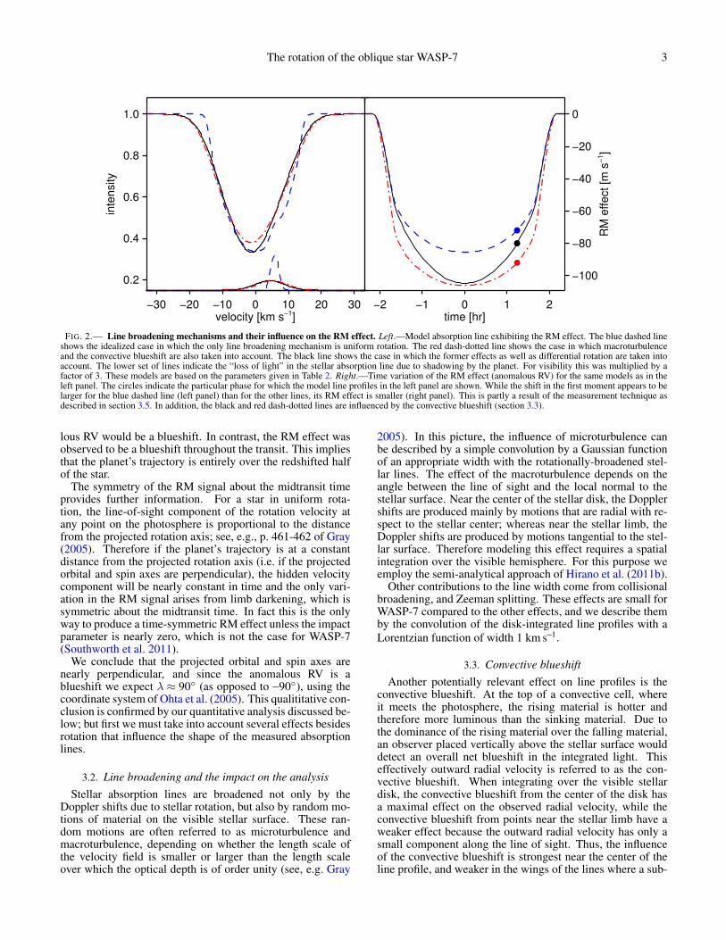
FIG. 2.— Line broadening mechanisms and their influence on the RM effect. Left.—Model absorption line exhibiting the RM effect. The blue dashed lineshows the idealized case in which the only line broadening mechanism is uniform rotation. The red dash-dotted line shows the case in which macroturbulenceand the convective blueshift are also taken into account. The black line shows the case in which the former effects as well as differential rotation are taken intoaccount. The lower set of lines indicate the “loss of light” in the stellar absorption line due to shadowing by the planet. For visibility this was multiplied by afactor of 3. These models are based on the parameters given in Table 2. Right.—Time variation of the RM effect (anomalous RV) for the same models as in theleft panel. The circles indicate the particular phase for which the model line profiles in the left panel are shown. While the shift in the first moment appears to belarger for the blue dashed line (left panel) than for the other lines, its RM effect is smaller (right panel). This is partly a result of the measurement technique asdescribed in section 3.5. In addition, the black and red dash-dotted lines are influenced by the convective blueshift (section 3.3).

lous RV would be a blueshift. In contrast, the RM effect wasobserved to be a blueshift throughout the transit. This impliesthat the planet’s trajectory is entirely over the redshifted halfof the star.

The symmetry of the RM signal about the midtransit timeprovides further information. For a star in uniform rota-tion, the line-of-sight component of the rotation velocity atany point on the photosphere is proportional to the distancefrom the projected rotation axis; see, e.g., p. 461-462 of Gray(2005). Therefore if the planet’s trajectory is at a constantdistance from the projected rotation axis (i.e. if the projectedorbital and spin axes are perpendicular), the hidden velocitycomponent will be nearly constant in time and the only vari-ation in the RM signal arises from limb darkening, which issymmetric about the midtransit time. In fact this is the onlyway to produce a time-symmetric RM effect unless the impactparameter is nearly zero, which is not the case for WASP-7(Southworth et al. 2011).

We conclude that the projected orbital and spin axes arenearly perpendicular, and since the anomalous RV is ablueshift we expect λ ≈ 90 (as opposed to −90), using thecoordinate system of Ohta et al. (2005). This qualititative con-clusion is confirmed by our quantitative analysis discussed be-low; but first we must take into account several effects besidesrotation that influence the shape of the measured absorptionlines.

3.2. Line broadening and the impact on the analysisStellar absorption lines are broadened not only by the

Doppler shifts due to stellar rotation, but also by random mo-tions of material on the visible stellar surface. These ran-dom motions are often referred to as microturbulence andmacroturbulence, depending on whether the length scale ofthe velocity field is smaller or larger than the length scaleover which the optical depth is of order unity (see, e.g. Gray

2005). In this picture, the influence of microturbulence canbe described by a simple convolution by a Gaussian functionof an appropriate width with the rotationally-broadened stel-lar lines. The effect of the macroturbulence depends on theangle between the line of sight and the local normal to thestellar surface. Near the center of the stellar disk, the Dopplershifts are produced mainly by motions that are radial with re-spect to the stellar center; whereas near the stellar limb, theDoppler shifts are produced by motions tangential to the stel-lar surface. Therefore modeling this effect requires a spatialintegration over the visible hemisphere. For this purpose weemploy the semi-analytical approach of Hirano et al. (2011b).

Other contributions to the line width come from collisionalbroadening, and Zeeman splitting. These effects are small forWASP-7 compared to the other effects, and we describe themby the convolution of the disk-integrated line profiles with aLorentzian function of width 1 km s−1.

3.3. Convective blueshiftAnother potentially relevant effect on line profiles is the

convective blueshift. At the top of a convective cell, whereit meets the photosphere, the rising material is hotter andtherefore more luminous than the sinking material. Due tothe dominance of the rising material over the falling material,an observer placed vertically above the stellar surface woulddetect an overall net blueshift in the integrated light. Thiseffectively outward radial velocity is referred to as the con-vective blueshift. When integrating over the visible stellardisk, the convective blueshift from the center of the disk hasa maximal effect on the observed radial velocity, while theconvective blueshift from points near the stellar limb have aweaker effect because the outward radial velocity has only asmall component along the line of sight. Thus, the influenceof the convective blueshift is strongest near the center of theline profile, and weaker in the wings of the lines where a sub-

4 Albrecht et al. 2011

0.990

0.995

1.000

relativeflux

−0.002

−0.001

0.000

0.001

0.002

O−C

−2 0 2 4Time [hr]

FIG. 3.— Photometry of WASP-7 transits. The upper panel shows thelight curve obtained by Southworth et al. (2011) in the Gunn I filter, and ourbest-fitting model. The lower panel shows the residuals between the data andbest-fitting model.

stantial portion of the light originates from the stellar limb.Therefore, the disk-integrated light has not only an overall

Doppler shift but also an asymmetry in the stellar absorptionlines. To describe this, we employ the model of Shporer &Brown (2011). This model captures the first-order effects ofthe convective blueshift but ignores a higher-order asymme-try in the absorption lines: the line cores are formed relativelyhigh in the photosphere where turbulent motions may be lessimportant. As WASP-7 is a relatively hot star, with high turbu-lent velocities, it seems appropriate to ignore the latter effect(see Figure 17.15 in Gray 2005).

3.4. Differential rotationWhen analyzing the RM effect researchers normally as-

sume the eclipsed star is rotating uniformly (no differentialrotation). In the case of WASP-7, the planet’s trajectory is ev-idently perpendicular to the projected stellar equator (see sec-tion 3.1), and therefore spans a wide range of stellar latitudes,and the effects of differential rotation might be expected to beespecially important. Ignoring the possibility of differentialrotation might lead to a systematic error in the measurementof the projected obliquity. For a well-aligned system (λ≈ 0)the effect is much less important because the planet probesonly a small range of stellar latitudes over the course of thetransit (see also Gaudi & Winn 2007).

We have limited empirical knowledge of differential rota-tion profiles in stars other than the Sun, and therefore we havelimited ability to predict the impact of differential rotation onour observation of WASP-7. One relevant study is by Rein-ers & Schmitt (2003), who examined differential rotation inslowly-rotating stars (vsin i? . 20 km s−1). In their sample, allstars having a logR′HK index between −4.80 and 4.65 showedsigns of differential rotation, while more active stars had nodiscernible differential rotation. Their sample did not includeany quieter stars (logR′HK < −4.80). In this context, we shouldexpect significant differential rotation for WASP-7, which ro-tates more slowly then 20 km s−1 (Hellier et al. 2009), and hasa low activity index logR′HK of −4.981 (H. Knutson, priv. com-munication, 2011). We adopt the parameterization used by

60 70 80 90 100 110 120λ [deg]

10

12

14

16

18

20

v si

n i [

km s

−1 ]

60 70 80 90 100 110 1200

2•104

4•104

6•104

8•104

1•105

0 2.0•104 4.0•104 6.0•104 8.0•104 1.0•105 1.2•105

10

12

14

16

18

20

FIG. 4.— Results for v sin i? and λ, based on our MCMC analysis in theWASP-7 system. The gray scale indicates the posterior probability den-sity, marginalized over all other parameters. The contours represent the 2-D68.3%, 95%, and 99.73% confidence limits. The one-dimensional marginal-ized distributions are shown on the sides of the contour plot.

Reiners & Schmitt (2003) and others,

Ω(l) = Ωeq(1 −αsin2 l). (1)

Here l denotes stellar latitude and Ωeq the angular rotationspeed at the equator. α is a dimensionless parameter whichdescribes the degree of differential rotation. An α of 0 wouldindicates uniform rotation and an α of 0.2 corresponds to Sun-like differential rotation. See also Hirano et al. (2011a), whoused the RM effect to set an upper limit on the stellar differ-ential rotation in the XO-3 system.

3.5. Modeling the anomalous RVIn order to develop a model for the anomalous RV produced

by the RM effect, we must take into account two other ef-fects: (1) the stellar absorption lines recorded by the spectro-graph are further broadened by the PSF of the spectrograph;and (2) the measured RVs represent the output of a Doppler-measuring code, which is akin to finding the peak of a cross-correlation between a stellar template spectrum obtained out-side the transit, and a spectrum observed during the transit.Some researchers neglect the second point, and model theanomalous RV as the shift in the first moment of the modelabsorption line rather than as the shift in the peak of the cross-correlation function. Depending on the system parametersthis can lead to systematic errors in the derived parameters(Hirano et al. 2010, 2011b).

Hirano et al. (2011b) developed an analytical descriptionfor the shift in the cross-correlation peak as a function of thetransit parameters, the stellar rotation velocity and obliquity,the microturbulent and macroturbulent velocities, the differ-ential rotation profile, and the PSF width of the spectrograph.We use their approach to model the obtained RVs during tran-sit and also include a model as described above for the con-vective blueshift. See Figure 2 for an illustration of how theabove described effects change the line shape and the timevariation of the RM effect.

3.6. Other RV variation sourcesTo this point we have only discussed changes in the RVs due

to the transit. To successfully model the RM effect we also

The rotation of the oblique star WASP-7 5

TABLE 2PARAMETERS OF THE WASP-7 SYSTEM

Parameter Values

Parameters mainly derived from photometry

Midtransit time Tc [BJDTDB−2 400 000] 55446.635 ± 0.0003Period, P [days] 4.9546416 ± 0.0000035cos io 0.05 ± 0.02Fractional stellar radius, R?/a 0.109 ± 0.011

0.006Fractional planetary radius, Rp/R? 0.096 ± 0.001u1+u2 0.34 ± 0.08

Parameters mainly derived from RVs

Velocity offset, [m s−1] 34 ± 5Linear slope during transit night, a1 [m s−1] −95 ± 41Quadratic slope during transit night, a2 [m s−1/day] 500 ± 310√

v sin i? sinλ [km s−1] 3.7 ± 0.3√v sin i? cosλ [km s−1] 0.24 ± 0.56

Macro turbulence parameter, ζ [km s−1] 6.4 ± 1.u1rm+u2rm 0.92 ± 0.06differential rotation parameter, α 0.45 ± 0.11cos i? 0.18 ± 0.43

Indirectly derived parameters

Orbital inclination, io [] 87.2 ± 0.91.2

Full duration, T14 [hr] 4.12 ± 0.090.06

Ingress or egress duration, T12 [min] 27 ± 69

Projected stellar rotation speed, v sin i? [km s−1] 14 ± 2Projected spin-orbit angle, λ [] 86 ± 6

need to model the change in radial velocity due to the orbitalmotion of the star. In addition, as we will see in section 4,WASP-7 shows a high level of RV noise on a timescale ofdays, which will introduce trends in the RV over the courseof the transit night. Therefore our model allows for RV trendsthat are linear or quadratic functions of time, in addition to theRM effect and orbital motion. The physical interpretation ofthese trends is discussed in section 4.

3.7. Quantitative AnalysisNow that all the ingredients of our model have been intro-

duced, we describe the various parameters in detail. The Ke-plerian orbital motion of the star is specified by the period(P), the time of inferior conjunction (Tc), the semi-amplitudeof the projected stellar reflex motion (K?), and a velocity off-set (γ). Initially we assume the orbit to be circular, as Hel-lier et al. (2009) found no sign of an orbital eccentricity (al-though see Section 4). We also allow for additional linear andquadratic RV trends (a1 and a2) on the transit night,

RV (t) = γ+RVOrbit(t)+RVRM(t)+a1∗(t −t0)+a2∗(t −t0)2 . (2)

Here RVOrbit(t) and RVRM(t) represent the radial velocitiescaused by the orbital motion and the RM effect. t0 is a pointin time near the middle of our observation sequence. Sinceallowing for these trends we have relinquished any power toconstrain K? with the data, so we fix K? at the value reportedby Hellier et al. (2009).

The amount of light blocked at any given phase of the tran-sit depends on the location of the chord of the planet’s pathover the stellar disk, which is parameterized by the cosine of

the orbital inclination (cos io), the radius of the star in unitsof the orbital semimajor axis (R?/a), and the radius of theplanet relative to the stellar radius (Rp/R?). We use quadraticlimb darkening parameters u1rm and u2rm to parameterize therelative intensity of the stellar surface in the wavelength re-gion of 5000-6200 Å, the spectral region in which the RVs aremeasured. We chose limb-darkening coefficients u1rm = 0.3,u2rm = 0.35, based on the tables of Claret (2004). We allowedu1rm +u2rm to vary freely and held fixed u1rm −u2rm at the tabu-lated value of −0.05, since the difference is only weakly con-strained by the data (and in turn has little effect on the otherparameters).

We parametrize the projected spin-orbit angle and the pro-jected stellar rotation by the quantities

√vsin i? cosλ and√

vsin i? sinλ, rather than vsin i? and λ. We do this becauseour chosen parameters are less strongly correlated (e.g. Al-brecht et al. 2011). Our macroturbulence model was that ofGray (2005), assuming equal surface fractions of radial andtangential velocities, with a macroturbulence parameter ζ sub-ject to a Gaussian prior of 6.4± 1.0 km s−1. This representsour expectation for a star of WASP-7’s effective temperature(Gray 1984). To model the convective blueshift we assumedan outward blueshift of 1 km s−1 at all positions on the star(Shporer & Brown 2011, and references therein). We furtherinclude α, the parameter which governs the strength of differ-ential rotation, and the stellar inclination towards the observer(i?) as free parameters. As Reiners & Schmitt (2003) foundno star with α

√sin i? greater ≈ 0.4 (see their Figure 16) we

also impose a prior on α which is flat until 0.4 and then fallsoff as a Gaussian function with a standard deviation of 0.1.

Finally, we must specify the width of a Gaussian functionrepresenting the width of the lines due to both microturbu-lence and the PSF of the spectrograph. We chose σ = 3 km s−1

for this purpose. Also, to represent the natural broadeningof the lines we used a Lorentzian function with a width of1 km s−1 (see also Hirano et al. 2011b).

Additional information on the transit geometry comes froma transit light curve recently obtained by Southworth et al.(2011). They made their de-trended light curve available viaVizieR. They also gave an updated transit ephemeris for thesystem, which is derived from the WASP discovery data incombination with the new light curve. We used those updatedresults for P and Tc as priors (see Equation 3). We also fittedthe light curve simultaneously with the RVs in order to pindown cos io, R?/a, and Rp/R?. We used the algorithm fromMandel & Agol (2002) to model the light curve which wasobtained in the Gunn I filter. From Claret (2004) we obtainedu1 = 0.17 and u2 = 0.36. We allowed u1 +u2 to vary freely, andheld u1 − u2 fixed at the tabulated value of −0.19.

To derive confidence intervals for the parameters we usedthe Markov Chain Monte Carlo algorithm. The likelihood wastaken to be exp(χ2/2), where χ2 was defined as:

χ2 =57∑i=1

[RVi(o) − RVi(c)

σRV,i

]2

+

1134∑j=1

[F j(o) − F j(c)

σF, j

]2

+

(Tc,BJD − 2455446.63493

0.000030

)2

+

(P − 4.d9546416

0.d0000035

)2

+

(ζ − 6.425kms−1

1kms−1

)2

+

0 if α≤ 0.4(α−0.4

0.1

)2 if α> 0.4, (3)

6 Albrecht et al. 2011

−0.05 1.05

−100

0

100

radi

al v

eloc

ity [m

s−

1 ]

CORALIE

HARPS

0.0 0.2 0.4 0.6 0.8 1.0phase

−50

0

50

O −

C [m

s−

1 ]

FIG. 5.— Orbital solution with zero eccentricity for WASP-7. The upperpanel shows RV observations as function of the orbital phase, with periastronat zero phase. The CORALIE RVs are indicated by filled symbols and theHARPS data are shown by open symbols. The lower panel shows the residu-als between data and best-fitting model.

The first two terms are sums-of-squares over the residualsbetween the observed (o) and calculated (c) values of the ra-dial velocity (RV) and relative flux (F). The following termsrepresent priors on some parameters, as mentioned above. Be-fore starting the chain we also added 10 m s−1 in quadrature tothe uncertainty of the PFS RVs to obtain a reduced χ2 close tounity. In making this step we assumed that the uncertaintiesin the RV measurements are uncorrelated and Gaussian.

Our results are presented in Table 2. The best fits to the RVsand photometry are shown in Figures 1 and 3. Figure 4 showsthe 2-d posterior density distribution for the two parametersof greatest interest for our study: λ and vsin i?.

For the parameters governed mainly by the photometricdata, our results are consistent with those obtained by South-worth et al. (2011). We will discuss the reliability of someof the parameters found by the RV data, in particular spectrallimb darkening, the evidence for differential rotation, and thestellar inclination in section 5.1, after investigating possiblereasons for the excess noise in the RV data in the followingsection.

4. STELLAR JITTER AND ORBITAL ECCENTRICITY

The out-of-transit RV gradient measured with the PFS issteeper than would be expected from the previously publishedspectroscopic orbit. That slope, and the known orbital period,imply an orbital velocity semiamplitude of K? ≈ 200 m s−1, instrong contrast to the published value of 97± 13 m s−1. (Seethe upper panel in Figure 1.)

Archival RV data from the CORALIE and HARPS spectro-graphs, obtained during various orbital phases, show a largescatter around the best orbital solution in excess of the mea-surement uncertainties. This type of excess noise is com-monly referred to as “stellar jitter”. In the following we willshortly investigate the timescale over which the RV scatter iscorrelated and test the possibility that the orbit is actually ec-centric.

4.1. Excess noiseWe turn first to the previously reported RVs. Eleven mea-

surements were obtained with CORALIE by Hellier et al.

0.25 180.00period [days]

2

4

6

8

10

po

we

r

0.05

0.01

0.001

1 10 100period [days]

2

4

6

8

10

po

we

r

0.05

0.01

0.001

FIG. 6.— Lomb-Scargle periodograms of the out-of-transit RVs. Theupper panel shows the power at different periods in the RV data of the twodata sets from CORALIE and HARPS. The highest peak occurs at the orbitalperiod. The lower panel shows the power in the RV data after the best fittingmodel was subtracted. Significant peaks occur at a period of one day, andits higher harmonics. Most likely this is a consequence of the diurnal timesampling of the RV observations.

(2009) and another eleven RVs were measured with HARPSby Pont et al. (2011). We fitted an orbital model to both datasets separately to determine the root mean square (rms) resid-ual between the data and the best-fitting model. A high rmswould indicate that our model neglects an effect which influ-ences the RVs, which for example could be activity of thestar itself. We find that the scatter of both the CORALIEand HARPS RVs is not only greater than what these instru-ments normally achieve on bright stars, also the rms of theHARPS data (33 m s−1) is slightly higher than the rms of theCORALIE RVs (31 m s−1). This is noteworthy as HARPSshould achieve a greater precision then CORALIE, if photonnoise is the limiting factor, as HARPS operates in conjunctionwith a 3.6 m telescope and CORALIE with a 1.2 m telescope.This suggests that an additional source of RV variations maybe present, which dominates the noise budget.

Next we fitted each dataset individually, assuming a circularorbit and adding a term in quadrature to the internal uncertain-ties to produce a reduced χ2 of unity. In making this step weassumed that the errors of the RV measurements are uncor-related and Gaussian. We needed to add 25 m s−1 in quadra-ture to the internal uncertainties of the eleven CORALIE dat-apoints and 33 m s−1 to the uncertainties of the eleven HARPSRVs.

Using those inflated uncertainties, we fitted both data setstogether, also assuming a circular orbit. Our fitting statisticwas

χ2 =22∑i=1

[RVi(o) − RVi(c)

σRV,i

]2

+

(Tc,BJD − 2455446.63493

0.000030

)2

+

(P − 4.d9546416

0.d0000035

)2

, (4)

making use of the ephemeris from Southworth et al. (2011).Figure 5 shows the phase-folded RV data. As expected

from the previous fits, the rms residual is 31.4 m s−1. Tounderstand this noise source it would be important to learnthe timescale over which the RV noise is correlated. Lookingat the Lomb-Scargle periodogram of the RV data, we find the

The rotation of the oblique star WASP-7 7

−90 0 90 ω [deg]

0.1

0.2

0.3

0.4

0.5

e

−100 0 1000

1•104

2•104

3•104

4•104

5•104

0 2.0•104 4.0•104 6.0•104 8.0•104 1.0•105 1.2•105

0.1

0.2

0.3

0.4

0.5

FIG. 7.— Constraints on the orbital eccentricity (e) and orientation (ω)of WASP-7 from HARPS and CORALIE data. The gray scale indicatesthe posterior probability density, marginalized over all other parameters. Thecontours represent the 2-d 68.3%, 95%, and 99.73% confidence limits. Theeccentricity is constrained to low values. For an orientation of ω ≈ |90|somewhat higher values of the eccentricity are allowed. That is particularlytrue for positive value of ω. The 1-d marginalized distributions are shown onthe sides of the contour plot.

most dominant peak at the orbital period of WASP-7b (Fig-ure 6, upper panel). After subtracting the best-fitting circular-orbit model, the periodogram of the residuals shows a strongpeak at a period of one day and its harmonics (Figure 6, lowerpanel). This is most likely a result of the timing of the ob-servations. Many observations were obtained on consecutivenights. Apart from this pattern, the periodogram is not veryinformative. An autocorrelation plot does not reveal addi-tional information.

The timing is different for the PFS observations. We ob-tained 37 data points during an interval of 7.5 hr. The rmsaround our solution including the orbital model, the linearand quadratic acceleration, and the RM effect is 11 m s−1 (Fig-ure 1). This relatively low scatter indicates that the correlationtime of the RV variations is longer then a few hours.

We note that WASP-7 is not the only early-type planet hoststar for which a large stellar jitter has been observed. RecentlyHartman et al. (2011) found that the two planet host stars inthe HAT-P-32 and HAT-P-33 systems have stellar jitter of ≈80 and 55 m s−1.

4.2. Orbital eccentricityOne possible contributing factor to the excess RV noise is

that the orbit is actually eccentric, in violation of our mod-eling assumption of a circular orbit. To investigate this pos-sibility we repeated the MCMC analysis but allowed the or-bital eccentricity (e) and the argument of periastron (ω) to befree parameters. Our stepping parameters were

√esinω and√

ecosω, which have less correlated uncertainties for smalleccentricity, and which correspond to a flat prior in e.

Using the likelihood based on Equation 4, we derived theposterior probability, which is displayed in the ω–e plane inFigure 7. The rms for the best fitting eccentric solution is with30.9 m s−1, only moderately smaller than for the circular-orbitmodel. We can see from Figure 7 that there is no clear de-tection of an eccentric orbit and that solutions with e & 0.2are generally disfavored except for values of ω near 90,

−90 0 90 ω [deg]

0.1

0.2

0.3

0.4

0.5

e

−100 0 1000

5.0•103

1.0•104

1.5•104

2.0•104

2.5•104

3.0•104

0 2.0•104 4.0•104 6.0•104 8.0•104 1.0•105 1.2•105

0.1

0.2

0.3

0.4

0.5

FIG. 8.— Results for orbital eccentricity using synthetic data. Similarto Figure 7 but this time for an MCMC analysis of a synthetic data set whichwas derived from a circular-orbit model. The results indicate that higher ec-centricities are allowed for ω near 90 or −90.

for which somewhat larger eccentricities are allowed. Suchan argument of periastron would indicate for transiting sys-tems a semi-major axis closely aligned with the line of sight(LOS). Interestingly, such an orbital orientation would lead toa steeper RV slope during the transit night, which is indeedwhat was observed with the PFS.

However, the peak in the probability density near ω ≈ 90should not be taken as evidence that the orbit really does havethis orientation. This is probably just the result of the factthat RV studies are better at constraining

√e× cosω than√

e× sinω, and consequently we expect the confidence in-terval for e to be larger for ω close to |90|. Such an orbitalconfiguration would lead to symmetric RV curves even foran eccentric orbit, i.e., the RV amplitudes at the quadratureswould not differ.

To investigate this point further we conducted numericalexperiments similar to those carried out by Laughlin et al.(2005) for the HD 209458 system. We created simulated RVdatasets with the same time stamps as the CORALIE andHARPS data sets. For this we assumed a circular orbit withthe parameters of the WASP-7 system. We then added Gaus-sian perturbations to the model RVs, adopting a 1σ uncer-tainty of 33 m s−1, and then used the same MCMC analysisfor these mock data as was used for the real data sets. A typ-ical 2-d posterior resulting from this experiment is shown inFigure 8.

We found that greater values of e are permitted for orbitalorientations of ≈ |90|. This should make us suspicious ofany low-SNR detection of an orbital eccentricity with an ωof ≈ |90|. We conclude that the out-of-transit RVs give noindication of an eccentric orbit for WASP-7. This is in linewith the upper limit e< 0.25 found by Pont et al. (2011). Wenote that the ω-dependent sensitivity to e is very similar tothe vsin i?-dependent sensitivity to λ that was explicated byAlbrecht et al. (2011), for low-SNR studies of the RM effect.In that case, higher values of the stellar rotation rate (vsin i)are allowed for λ≈ 0 and≈ 180, even when the underlyingsignal has no RM effect at all.

5. DISCUSSION

8 Albrecht et al. 2011

5.1. Differential rotation parametersOur model took into account the possible effects of differ-

ential rotation, through the parameters α and i?. We foundthat the upper boundary of the posterior distribution for αis determined mainly by our prior. Specifically we foundα = 0.45± 0.11, with the prior enforcing α < 0.5 (see Ta-ble 2). If instead no prior is placed on α, then we found thatthe differential rotation parameter increases to values as highas 0.9, much higher than would be expected based on theoryand on observations of other stars.

This should make us suspicious. For |λ| close to 90, asis the case here, a parameter degeneracy exists between thelimb-darkening profile and the degree of differential rotation,because both of those phenomena produce changes to the RMeffect that are symmetric in time about the transit midpoint.Perhaps our assumptions are mistaken regarding the stellarlimb darkening within the effective observing bandpass. ForRM observations the effective observing bandpass is compli-cated to describe, depending as it does upon the density of I2absorption lines. Furthermore, there may be systematic dif-ferences between the limb darkening as observed in differentabsorption lines, and even within a single strong line, as dif-ferent parts of the absorption lines form in different depthsof the stellar photosphere. Nevertheless, the fitted value ofthe center-to-limb variation (u1rm + u2rm = 0.92± 0.06) is al-ready quite high; lowering this value would only cause α toconverge to larger values.

The data seem to be demanding a greater variation of theRM effect between the second and third contact than is deliv-ered by the expected amounts of limb darkening and differen-tial rotation. Some possible explanations are:

• The stellar jitter exhibits correlations on the timescaleof minutes to hours, which is not taken into account inour model. By fitting a linear and quadratic trend to theRVs, we have only taken into account correlations onlonger timescales.

• If WASP-7 is pulsating then velocity fields on the stellarsurface, due to the pulsations, might lead to a differentshape of the stellar absorption line than is created by ourmodel, which does not include pulsations. The planetwould occult during its transit different velocity com-ponents than expected. For this effect to be importantthe velocity fields do not need to change on a timescalecomparable to the transit.

• Another possibility is that our model of the convectiveblueshift is not correct. For hotter stars there exists a re-versed shape in the bisectors, although WASP-7 seemsto be securely located on the ’cool’ side of this ’granu-lation boundary’ (see Fig. 17.18 in Gray 2005).

With the present data we cannot determine if one of theseor another effect is responsible for the relatively strong vari-ations in the shape of the RM signal. One should thereforeview our particular results for the differential rotation, stellarinclination, and the spectroscopic limb darkening coefficientswith some skepticism. Including these effects, or some ef-fects with a similar functional form, is however important fora realistic uncertainty estimation of vsin i? and λ as we willdiscuss in the next section.

5.2. Stellar obliquity

0 50 100 150incl star [deg]

60

70

80

90

100

110

120

λ [d

eg]

0 50 100 1500

1•104

2•104

3•104

4•104

0 2•104 4•104 6•104 8•104 1•105

60

70

80

90

100

110

120

FIG. 9.— Dependency of λ on i?. The gray scale indicates the poste-rior probability density, marginalized over all other parameters. The con-tours represent the 2-d 68.3%, 95%, and 99.73% confidence limits. The 1-dmarginalized distributions are shown on the sides of the contour plot. Onecan see the strong correlation between λ and i?. This correlation vanishes ifno differential rotation is present.

As expected from the qualitative discussion we find λ =86± 6, which is consistent with 90. The projected stellarspin axis is lying nearly within the orbital plane.

We did not use the measurement of the projected rotationalvelocity (vsin i? = 17±2 km s−1) by Hellier et al. (2009) as aprior constraint. This is because it is not clear what value ofmacroturbulence was assumed by those authors, and also be-cause if differential rotation is present then a systematic errorcould be introduced.

The lack of knowledge on differential rotation and the stel-lar inclination did lead to an increased confidence interval forλ. This can be seen from the Figures 4 and 9. When the stel-lar inclination departs from 90, the planet covers higher stel-lar latitudes, which have decreased rotational velocities (andtherefore a decreased RM effect) either at the beginning orend of the transit. This forces a higher vsin i? and a changein λ to compensate for the asymmetry in the transit RV curve.This degeneracy could be broken if we would have indepen-dent information on the stellar inclination.

To estimate sin i? we can use the technique of Schlauf-man (2010), involving a comparison of the measured value ofvsin i? with the expected value of v for a star of the given ageand mass. Schlaufman found for WASP-7 a rotation statisticΘ = −3.4, indicating that WASP-7 rotates faster then expectedfor its age and mass. A Θ near 0 would indicate that the mea-sured vsin i? is consistent with the expected rotation speed vfor a star of a given mass and age. A Θ larger then 0 wouldindicate an inclination of the stellar spin axis towards the ob-server.

We repeat his analysis with the new values for vsin i?, foundhere using the RM effect (Table 2), and the new mass, radiusand age values from Southworth et al. (2011). With these weobtain an expected v of 11± 4 km s−1 and a rotation statisticΘ of −0.8. This indicates that the projected rotation speedis consistent with a sin i? of ≈ 1 There is no indication of aninclination of the stellar spin axis towards the observer.

This knowledge could be used as prior knowledge, or morecorrectly used in the model itself to decrease the uncertaintyin the projected obliquity. However as WASP-7 is at the up-

The rotation of the oblique star WASP-7 9

per end of the mass range for which Schlaufman (2010) cal-culated his rotation, mass, age relationship and because of thecomplications due to differential rotation for which his rela-tion was not calibrated, we decided not to use this knowledgeto reduce the uncertainty in λ.

5.3. Stellar jitterAnalyzing the bisectors of the obtained spectra might lead

to a reduced scatter, as was done for HAT-P-33 by Hartmanet al. (2011). In particular the data taken during the transitnight might be informative as the change in the bisectors willbe correlated over the course of the night.

If during some nights several RVs would have been ob-tained then the uncertainty in the orbital parameters of WASP-7 could be reduced in a similar approach to that used byHatzes et al. (2010) for CoRoT-7. They used data obtainedduring one night to constrain a part of the orbit and allowedfor a drift between different nights. However this approach re-quires a substantial amount of data and its success depends onthe timescale over which the jitter is correlated, with shortercorrelation timescales being advantageous.

As we are mainly interested in the systems obliquity weonly note here that the relation by Saar et al. (2003) employ-ing a correlation between vsin i? and stellar jitter, leads to anexpected jitter of 34 m s−1, similar to the measured value.

6. SUMMARY OF CONCLUSIONS

We find that in the WASP-7 system the stellar spin axis isstrongly misaligned with the planet’s orbital axis, by 86±6as projected on the sky. This observation strengthens the cor-relation found by Winn et al. (2010) and lends support to the

idea that systems with close giant planets generally started outwith a very broad range of obliquities, and that the observedlow obliquities of many systems are a consequence of tidaldissipation.

Differential rotation and its imprint on the RM effect holdsthe promise of measuring not only the projections of stellarobliquities, but also the stellar inclinations. However, withthe current measurement precision and uncertainties in otherparameters such as limb darkening, no secure detection ofdifferential rotation in WASP-7 can be made. We originallythought that WASP-7 might present a good testbed to searchfor differential rotation via the RM effect, as the misalignmentof 90 maximises the RM signal originating from differentialrotation. However for this angle the signal from differentialrotation is also strongly correlated with stellar limb darken-ing. In addition WASP-7 displays a high degree of stellar jit-ter. Therefore a system with a quiet star and a more moderatemisalignment might be better suited to search for signs of dif-ferential rotation in the RM signal.

S.A. thanks the Harvard-Smithsonian Center for Astro-physics, where this manuscript was begun, for its hospi-tality. S.A. acknowledges support by a Rubicon fellow-ship from the Netherlands Organization for Scientific Re-search (NWO) during parts of this project. J.N.W. acknowl-edges support from a NASA Origins grant (NNX09AD36G).T.H. is supported by Japan Society for Promotion of Sci-ence (JSPS) Fellowship for Research (DC1: 22-5935). Thisresearch has made use of the Simbad database located athttp://simbad.u-strasbg.fr/.

REFERENCES

Albrecht, S., Reffert, S., Snellen, I., Quirrenbach, A., & Mitchell, D. S.2007, A&A, 474, 565, ADS, 0708.2918

Albrecht, S. et al. 2011, ApJ, 738, 50, ADS, 1106.2548Butler, R. P., Marcy, G. W., Williams, E., McCarthy, C., Dosanjh, P., &

Vogt, S. S. 1996, PASP, 108, 500, ADSChatterjee, S., Ford, E. B., Matsumura, S., & Rasio, F. A. 2008, ApJ, 686,

580, ADS, arXiv:astro-ph/0703166Claret, A. 2004, A&A, 428, 1001, ADSCollier Cameron, A., Bruce, V. A., Miller, G. R. M., Triaud, A. H. M. J., &

Queloz, D. 2010, MNRAS, 403, 151, ADS, 0911.5361Crane, J. D., Shectman, S. A., Butler, R. P., Thompson, I. B., Birk, C., Jones,

P., & Burley, G. S. 2010, in SPIE Conference Series, Vol. 7735, 170, ADSCresswell, P., Dirksen, G., Kley, W., & Nelson, R. P. 2007, A&A, 473, 329,

ADS, 0707.2225Fabrycky, D., & Tremaine, S. 2007, ApJ, 669, 1298, ADS, 0705.4285Gaudi, B. S., & Winn, J. N. 2007, ApJ, 655, 550, ADS, 0608071Gray, D. F. 1984, ApJ, 281, 719, ADS—. 2005, The Observation and Analysis of Stellar Photospheres, 3rd Ed.

(ISBN 0521851866, Cambridge University Press), ADSHartman, J. D. et al. 2011, ArXiv e-prints, ADS, 1106.1212Hatzes, A. P. et al. 2010, A&A, 520, A93, ADS, 1006.5476Hébrard, G. et al. 2008, A&A, 488, 763, ADS, 0806.0719Hellier, C. et al. 2009, ApJ, 690, L89, ADS, 0805.2600Hirano, T., Narita, N., Sato, B., Winn, J. N., Aoki, W., Tamura, M., Taruya,

A., & Suto, Y. 2011a, ArXiv e-prints, ADS, 1108.4493Hirano, T., Suto, Y., Taruya, A., Narita, N., Sato, B., Johnson, J. A., & Winn,

J. N. 2010, ApJ, 709, 458, ADS, 0910.2365Hirano, T., Suto, Y., Winn, J. N., Taruya, A., Narita, N., Albrecht, S., &

Sato, B. 2011b, ArXiv e-prints, ADS, 1108.4430

Johnson, J. A., Winn, J. N., Albrecht, S., Howard, A. W., Marcy, G. W., &Gazak, J. Z. 2009, PASP, 121, 1104, ADS, 0907.5204

Laughlin, G., Marcy, G. W., Vogt, S. S., Fischer, D. A., & Butler, R. P. 2005,ApJ, 629, L121, ADS

Lin, D. N. C., Bodenheimer, P., & Richardson, D. C. 1996, Nature, 380, 606,ADS

Mandel, K., & Agol, E. 2002, ApJ, 580, L171, ADS, 0210099Maxted, P. F. L., Koen, C., & Smalley, B. 2011, ArXiv e-prints, ADS,

1108.0349Nagasawa, M., Ida, S., & Bessho, T. 2008, ApJ, 678, 498, ADS, 0801.1368Ohta, Y., Taruya, A., & Suto, Y. 2005, ApJ, 622, 1118, ADS,

astro-ph/0410499Pont, F., Husnoo, N., Mazeh, T., & Fabrycky, D. 2011, MNRAS, 414, 1278,

ADS, 1103.2081Reiners, A., & Schmitt, J. H. M. M. 2003, A&A, 398, 647, ADSSaar, S. H., Hatzes, A., Cochran, W., & Paulson, D. 2003, in The Future of

Cool-Star Astrophysics: 12th Cambridge Workshop on Cool Stars, StellarSystems, and the Sun, ed. A. Brown, G. M. Harper, & T. R. Ayres,Vol. 12, 694–698, ADS

Schlaufman, K. C. 2010, ApJ, 719, 602, ADS, 1006.2851Shporer, A., & Brown, T. 2011, ApJ, 733, 30, ADS, 1103.0775Simpson, E. K. et al. 2011, MNRAS, 414, 3023, ADS, 1011.5664Southworth, J. et al. 2011, A&A, 527, A8, ADS, 1012.5181Triaud, A. H. M. J. 2011, A&A, 534, L6, ADS, 1109.5813Triaud, A. H. M. J. et al. 2010, A&A, 524, A25, ADS, 1008.2353Winn, J. N., Fabrycky, D., Albrecht, S., & Johnson, J. A. 2010, ApJ, 718,

L145, ADS, 1006.4161Winn, J. N. et al. 2011, AJ, 141, 63, ADS, 1010.1318Winn, J. N., Johnson, J. A., Albrecht, S., Howard, A. W., Marcy, G. W.,

Crossfield, I. J., & Holman, M. J. 2009, ApJ, 703, L99, ADS, 0908.1672