a hobo syndrome? mobility, wages, and job turnoverlm25/le-2004.pdfa hobo syndrome? mobility, wages,...

www.elsevier.com/locate/econbase

Labour Economics 11 (2004) 191–218

A hobo syndrome? Mobility, wages, and job turnover

Lalith Munasinghea,*, Karl Sigmanb

aDepartment of Economics, Barnard College, Columbia University, 3009, Broadway, New York, NY 10027, USAbDepartment of Industrial Engineering and Operations Research, Columbia University, USA

Received 21 August 2001; received in revised form 1 January 2003; accepted 30 May 2003

Abstract

We present an analysis of labor mobility as a predictor of wages and job turnover. Data from the

National Longitudinal Surveys of Youth show that workers with a history of less frequent job

changes (stayers) earn higher wages and change jobs less frequently in the future than their more

mobile counterparts (movers). These mobility effects on wages and turnover are stronger among

more experienced workers, are highly robust across various model specifications, and persist despite

corrections for unobserved individual fixed effects. In the second half of the paper we present a

simple two period stochastic model of job mobility to study wages across movers and stayers. The

model, incorporating salient features of human capital and job search, shows that whether stayers

earn more than movers depend on the distribution of outside wage offers and firm-specific wage

growth rate. Incorporating heterogeneity of wage growth rates among jobs increases the likelihood

that stayers earn more than movers.

D 2003 Published by Elsevier B.V.

JEL classification: J33; J41; J63

Keywords: Movers and stayers; Wages; Turnover

1. Introduction

The relationship between the frequency of past job1 changes (mobility) and other labor

market outcomes, such as wages and future job changes (turnover), is a widely recognized

phenomenon. In particular, the positive correlation between mobility and turnover, and the

0927-5371/$ - see front matter D 2003 Published by Elsevier B.V.

doi:10.1016/j.labeco.2003.05.001

* Corresponding author. Tel.: +1-212-854-5652; fax: +1-212-854-8947.

E-mail address: [email protected] (L. Munasinghe).1 Throughout the paper, job is synonymous with employer since we do not distinguish between job levels

within firms and other internal labor market phenomena.

L. Munasinghe, K. Sigman / Labour Economics 11 (2004) 191–218192

negative correlation between mobility and wages, are well-known empirical regularities

across many disciplines. In the sociological literature these mobility patterns were

explained by the so-called mover–stayer model (Blumen et al., 1955). The argument,

in economic parlance, was based on ‘‘individual fixed effects:’’ some workers (identified

as movers) are inherently more likely to move between jobs than some others (identified as

stayers); and it was further presumed that movers are less productive than stayers. In the

organizational psychology literature this same phenomenon was colorfully labelled the

‘‘hobo syndrome,’’ and described as the ‘‘periodic itch to move from a job in one place to

some other job in some other place’’ (Ghiselli, 1974). It was believed that the hobo’s

wanderlust derived from instinctive impulses.

Although these mobility facts have been extensively documented in the recent literature

on job mobility and wages,2 economic studies have yet to fully wrestle with the widely

accepted view, even if only implicitly, that these empirical regularities are simply a

consequence of an inherent ‘‘itch’’ or individual fixed effect. Since many of these mobility

studies were based on cross-sectional data,3 the more precise interpretive question is

whether mobility effects on wages and turnover are a mere consequence of some

unobserved individual characteristic or whether the history of job mobility reflects more

fundamental search and investment processes that might be systematically linked to

current labor market outcomes. As a consequence, the primary objective of this paper is to

re-establish these mobility effects on current wages and turnover, and especially, to address

whether these observed mobility patterns persist after accounting for individual fixed

effects; or, put differently, to address whether heterogeneity of some unobserved individual

characteristic can fully account for mobility effects on wages and turnover.

Data from the National Longitudinal Surveys of Youth (NLSY) are ideally suited to

study the role of mobility in predicting wages and turnover. Since we observe the entire

early work histories of the vast majority of our respondents and because information on

the total number of jobs ever held is available, we can directly correlate frequency of past

job changes with current wages and the likelihood of future job separations, respectively.

In addition, the panel nature of the data allows us to implement econometric procedures to

account for individual fixed effects. The NLSY data also contain rich information on a

variety of individual, job, geographic, and other work related characteristics, and as a

consequence, we include an extensive array of control variables in our regression

analyses.

To preview our main findings: high mobility is associated with low wages, especially

among more experienced workers. This negative effect persists despite corrections for

individual fixed effects. The effects of mobility on turnover closely parallel the effects of

mobility on wages. Mobility is positively associated with the likelihood of a future job

separation. This positive effect is stronger among more experienced workers, is highly

robust to various model specifications and corrections for individual fixed effects, and

holds across both quits and layoffs. Hence, hypotheses based on individual fixed effects,

2 Mincer and Jovanovic (1981), Bartel and Borjas (1981), Light and McGarry (1998).3 Except for the Light and McGarry (1998) analysis, which is based on the National Longitudinal Surveys of

Youth data, the same panel that we use in our study.

L. Munasinghe, K. Sigman / Labour Economics 11 (2004) 191–218 193

including the mover–stayer model and the hobo syndrome, are implausible explanations

for mobility effects on wages and turnover.

A second concern of the paper is to develop a simple two period model of job

mobility to compare wages across movers and stayers. The objective of this analytical

effort is to ask whether a model based on job search and human capital can generate any

implications for wages of movers versus stayers without appealing to individual

heterogeneity of any stripe. The job search feature of the model is that workers search

from a stationary distribution of outside wage offers and receive a single offer every

period. Workers switch jobs if the outside wage offer is greater than the second period

wage in the incumbent firm. And the human capital feature is that the second period

wage is higher than the first period wage (in the incumbent firm) because of firm-specific

wage growth. Although this simplistic model creates a systematic link between mobility

and wages, the comparison of wages between movers and stayers remains indeterminate

because whether stayers earn more than movers depend on the specifics of the

distribution of wage offers and the wage growth rate. The intuition is straightforward.

Indeed, movers do not receive wage increases due to within-job wage growth (as stayers

do) because they move. But movers do receive wage increases because they move to

more lucrative jobs. Hence, the precise wage differential between stayers and movers

depends on which of these two effects dominate. However, introducing heterogeneity of

wage growth rates among jobs increases the likelihood that stayers earn more than

movers because those in high wage growth jobs are less likely to move and more likely

to have higher second period wages.

The remainder of the paper is organized as follows. In the next section entitled ‘‘Related

literature’’ we discuss in detail empirical and theoretical studies related to mobility, wages,

and turnover. Section 3 in various subparts presents the details of the empirical analysis of

mobility effects on wages and turnover. In Section 4 we present a simple two period model

of job mobility to rationalize why stayers earn more than movers. Section 5 concludes. A

bibliography is appended.

2. Related literature

The Achilles heal of the mover–stayer hypothesis is the claim that movers are less

productive than stayers, and thus, movers earn less than stayers. In the fairly recent

economics literature a variety of wage and turnover models have been designed to

explicitly incorporate heterogeneity of mobility and search costs. These models typically

lead to natural links between mobility and wages. For example, Black and Loewenstein

(1991) develop a three-period model based on heterogeneity of mobility costs and self-

enforcing contracts, and show, among various other results, that in the resulting

equilibrium previous turnover increases the probability of subsequent turnover, and job

changers systematically earn higher wages than job stayers. The authors argue that the

latter finding may be consistent with some specialized labor markets, such as the labor

market for academics. Note, however, that this prediction of their model is not supported

by many studies, including the findings in our paper, that find past turnover is negatively

correlated with wages.


Various other studies have modeled labor market outcomes, including wages and

turnover, as a function of quit propensities across women and men. Although some of

these papers, including Barron et al. (1993) and Kuhn (1993), are explicitly designed to

investigate differences in gender outcomes due to differences in quit propensities, the

models are easily adapted to study the links between mobility and wages due to

heterogeneity of individual quit propensities.

Although these economic models go beyond the simple mover–stayer hypothesis in

terms of endogenizing mobility and wages, two issues still remain. First, the theoretical

predictions of these models do not square with all of the empirical evidence on mobility

effects. Second, and more importantly, they are inconsistent with the recent empirical

evidence that corrects for individual fixed effects. As we have mentioned earlier, many of

the earlier studies on mobility (Mincer and Jovanovic, 1981; Bartel and Borjas, 1981) were

based on cross-sectional data, and hence, the observed correlations could, in principle, be

consistent with these models or the mover–stayer hypothesis. By contrast, recent

econometric work on the effects of mobility on wages (Light and McGarry, 1998) and

on turnover (Judge and Watanabe, 1995) have exploited the panel nature of their data to

control for unobserved, time invariant individual characteristics. The fact that mobility

remains a significant predictor of wages and turnover despite these heterogeneity

corrections is prima facie evidence not only against the mover–stayer model and the

hobo syndrome,4 but also against these equilibrium models because the purported links

between mobility, wages, and turnover are generated because of individual fixed effects—

i.e., on account of individual heterogeneity in terms of mobility and search costs. As a

consequence, a natural question to ask is whether there might be a structural relationship

between past mobility and current labor market outcomes, such as wages and turnover,

independently of unobserved individual fixed effects. As a consequence, our modeling

effort is to ask whether the standard workhorse theories of labor—search and human

capital—might have ramifications for mobility as a predictor of wages without appealing

to heterogeneity of individual fixed effects.

Although various adaptations of these workhorse theories are widely accepted as

providing an explanation for why wages increase with job tenure (and work experience),

and for why turnover rates decline with job tenure (and over the life cycle), neither search

nor human capital considerations alone seem to generate systematic links between

mobility and wages. A simple search model, where workers sample outside wage offers

from the same distribution in each time period, predicts that current wages are independent

of prior mobility (Burdett, 1978). That is, there is no systematic discrepancy between the

expected wages of movers and stayers,5 and thus also no systematic discrepancy between

the future turnover outcomes of movers and stayers. The job matching model (Jovanovic,

1979a) may appear to predict a negative correlation between mobility and wages, but

4 Judge and Watanabe (1995) claim that their evidence—those who quit numerous jobs in the past were

much less likely to survive on the job than those who quit few jobs (p. 220)—supports the hobo syndrome.

However, given that they account for unobserved heterogeneity this conclusion seems unwarranted. If some

individuals posses ‘‘internal impulses to migrate,’’ and if these impulses are time invariant, then accounting for

individual fixed effects should in principle nullify the effect of past mobility on future mobility.5 This result, however, is not robust. As Weiss and Landau (1984) show, the introduction of a cost of mobility

leads to a breakdown of this result.


Jovanovic explicitly notes in his article that the mismatch theory does not imply that

movers should do worse than stayers.6 Human capital theory predicts a negative

relationship between job mobility and investments in job specific skills,7 but these

considerations do not yield any ex ante predictions about the relative wages of movers

and stayers (Light and McGarry, 1998).

Since these considerations alone have never been developed into a model to explicitly

study mobility effects,8 our simple model in the paper attempts to formalize these basic

ideas to address whether past mobility is related to current wages. Of course, since these

ideas are not new, similar theoretical considerations have guided key empirical studies that

try to obtain unbiased estimates of rates of return to tenure (Topel, 1991) and estimates of

mobility wage gains (Antel, 1986). The first study argues that a comparison of wages of

stayers and movers will underestimate the ‘‘true’’ return to tenure (due to firm specific

training) because movers move to better paying jobs. The second study argues, conversely,

that a comparison of wages of movers and stayers will underestimate ‘‘true’’ mobility

wage gains (due to search effort) because wages of stayers grow due to firm specific

training. Clearly, these two arguments are flip sides of the same coin. But neither study

asks whether there is any systematic wage differential between stayers and movers, which

of course is the key question for us.9

Given that our model is centered around the idea of firm-specific wage growth, it is

important to address the recent empirical controversy about finding a tenure effect on

wages. The early empirical support for wage increases with job seniority was based on

evidence of positive cross-sectional association between seniority and earnings. However,

as Abraham and Farber (1987) and Altonji and Shakotko (1987) argue, this evidence is

insufficient to establish that earnings increase with seniority. For instance, if high wage

jobs (due to say heterogeneity of worker–firm match quality) are more likely to survive

than low wage jobs, then seniority will be positively correlated with high wages even

though individual wages do not rise with seniority. Using longitudinal data and corrections

for various potential sources of heterogeneity bias, both these studies find that the cross-

sectional return to tenure is a statistical artifact of heterogeneity bias, and that the true

wage return to tenure is small if not negligible. However, a later study by Topel (1991),

also using longitudinal data and accounting for selection due to optimal mobility

decisions, shows that wages do rise with seniority. A recent reassessment by Altonji

and Williams (1997) concludes that Topel over estimates the returns, and that wage returns

to tenure, across all these estimation procedures, are modest at best.10 It is important to

6 See Jovanovic (1979a), footnote 11 on p. 982.7 See Becker (1975) and Jovanovic (1979b).8 The models mentioned earlier are of course based on similar considerations. However, mobility effects in

these models are generated by explicitly assuming heterogeneity of search and mobility costs. Our objective is to

ask whether mobility effects can be generated without appealing to any such individual effect.9 Note that the biases identified in each of the two studies remain in force whether stayers earn more than

movers or vice versa. Simply, the issue of who earns more is equivalent to whether the within-job wage growth

effect on the wages of stayers dominates the search effect on the wages of movers.10 Other empirical studies also seem to support the view that wage returns to tenure might be small. For

example, Neal (1995) and Carrington (1993) present evidence to suggest that much of the tenure effect on wages

may in fact be an industry as opposed to a firm effect.


note, however, that dynamically consistent models of wage determination can imply small

wage returns to tenure despite substantial firm-specific skill accumulation (Munasinghe,

2001).

In an earlier paper, Munasinghe (2000) conjectured that in the presence of high and low

wage growth jobs it would be more likely that stayers earn more than movers. Hence we

extend our simple model with constant wage increase to incorporate heterogeneity of wage

growth rates among jobs, a cornerstone of human capital theory.11 The empirical evidence

on heterogeneity of wage growth rates among jobs is also somewhat controversial. Abowd

et al. (1999) find, using a large longitudinal French data source, that the estimated returns

to tenure are small, but that there is substantial variation in these estimated tenure slopes

across firms. Topel (1991) argues that heterogeneity of wage growth rates among jobs is

empirically unimportant because there is no evidence of serial correlation of within-job

wage increases. Note, however, that recent theoretical considerations show that serial

correlation of wage increases is an inappropriate test for wage growth heterogeneity

(Munasinghe, 2001). Perhaps more importantly, in a series of studies, Mincer (1986, 1988)

found that stayers receive more job training than movers, and that movers, despite the

gains to moving, do not catch up with wage levels of stayers. Although these are empirical

observations, they do suggest that mobility related findings might possibly be explained by

heterogeneous investments in firm specific human capital across individuals. We attempt

to provide a theoretical basis for these observations by explicitly showing, in the context of

our stochastic model, how heterogeneity of firm specific wage growth rates among jobs

makes it more likely for stayers to earn more than movers. The point is that to explain

wage differences across movers and stayers, heterogeneity of wage growth may be more

relevant than the size of the tenure effect on wages.

3. Empirical analysis

Our objective in this two part empirical analysis is to study the role of mobility, defined

as the ratio of jobs ever held to total labor market experience, as a predictor of current

wages and future turnover, respectively. Given the extensive array of information available

in the NLSY data, we can assess the net effect of mobility on wages and turnover after

controlling for a variety individual, job and other characteristics. Further, since the NLSY

is a panel data source, we can also make efforts to control for unobserved individual

heterogeneity in our estimation procedures. We begin this section with a brief discussion

of the estimation framework for analyzing the role of mobility in predicting wages and

turnover. In Section 3.2 we describe the NLSY data, construction of key variables, and

sample restrictions. The next subsection presents summary statistics and analysis of

mobility correlates. In Sections 3.4 and 3.5 we present our main results from wage and

turnover regressions, respectively, to study the effects of mobility on key labor market

outcomes.

11 For example, see Becker’s (1975) analysis of supply and demand for human capital for a variety of reasons

why human capital investments differ among individuals.

3.1. Estimation framework

The following discussion outlines the estimation framework to analyze the effects of

mobility on wages and turnover.12 First, consider a standard cross-section human capital

earnings equation augmented to include mobility as an additional explanatory variable:

wi ¼ Xib þ bmi þ a þ ei;

where w is log of real wages, X is a vector of observed worker, job and other character-

istics, m is the mobility rate, e is the error term, and all terms indexed by i pertain to worker

i. Since each worker is observed at several points in time, we can consider an alternative

specification of this regression model that explicitly incorporates heterogeneity or

individual fixed effects:

wit ¼ Xitb þ bmit þ zia þ eit:

The individual effect is zia where zi includes a constant term and an unobserved, time-

invariant individual specific variable. Hence the error component is composed of both an

individual specific effect and a white noise component. This formulation allows a

consideration of whether some unobserved individual characteristic is likely to be

correlated with both our measure of mobility and wages, and thus lead to a biased

estimate of the ‘‘true’’ mobility effect on wages under an OLS specification with pooled

data. A key empirical issue to resolve is whether the observed negative effect of mobility

on wages is simply due to a fixed individual effect, such as in the case of the mover–stayer

hypothesis, or whether this observed correlation is indicative of a structural or causal

linkage. The panel nature of our data allows us to get estimates of mobility effects after

correcting for potential bias on account of individual fixed effects.

The two standard procedures to handle heterogeneity with panel data are the so called

fixed and random effects models. In the former, the wage regression reduces to:

wit =Xitb + bmit + ai + eit, where ai is interpreted as an individual specific term that is

constant over time. In the estimation of this model, the constant individual term can be

correlated with the regressors, but it does not yield coefficient estimates for any of the time

invariant variables. The random effects model on the other hand generates coefficient

estimates for time invariant variables, but the restrictive assumption in this specification is

that the unobserved individual effect is uncorrelated with the other regressors. Since our

primary concern is to establish the mobility effect on wages, we present results from all

three model specifications—OLS, fixed and random effects models—to assess the

robustness of the mobility effect on wages.13

Estimating mobility effects on turnover raises further complications on account of the

fact that the dependent variable is dichotomous—whether a job separation occurs or not.


12 For a more detailed discussion of the issues involved in using panel data to address heterogeneity, see

Greene (2003).13 There are of course various tests to evaluate the fixed and random effects specification against the classical

pooled regression—i.e. whether there are individual effects. Further, there is also a Hauseman test to discriminate

between the fixed and random effects models. In Section 3.4 we discuss the implications of these test results for

our wage analyses.


The standard models for limited dependent variables are the linear probability model and

various nonlinear specifications, of which the Logit and Probit models are the best known.

A key issue again is whether these models can account for individual fixed effects in the

context of estimating a turnover model. Both the fixed effects and random effects models

discussed earlier can be adopted and amended to accommodate the fact that the dependent

variable is a dichotomous variable. Hence we use an extended binary choice framework

and estimate an individual effects model for panel data.

yit* ¼ Xita þ bmit þ li þ eit; i ¼ 1; . . . n; t ¼ 1; . . .Ti;

yit ¼ 1 if yit* > 0; and 0 otherwise:

The estimation of this model raises a few additional problems. For example, fixed

effects models can only be estimated on observations that do not have only positive or

negative outcomes. And since our data contain a large sample of individuals with such

observations this procedure is infeasible. However, a random effects model, given the

various caveats mentioned earlier, does not impose the same restriction and is thus

feasible. In our regression analyses we present results from three model specifications,

starting with a simple linear probability model, followed by a logit model, and finally a

random effects specification of the logit model.

3.2. Data and sample restrictions

We use NLSY panel data from 1979 to 1994 to study the role of prior mobility in

predicting current wages and future turnover rates. The NLSY tracks 12,686 young

women and men first interviewed in 1979. The availability of work histories of early

careers, including detailed information on job duration and separation, labor market

experience, annual earnings, number of total employers a person has ever worked for, and

other individual and job characteristics, make this data ideal for our empirical analyses of

mobility, wages, and turnover.

We only consider Current Population Survey (CPS) designated jobs in the NLSY.

Typically the CPS job is the main or more recent job, and more information is available

about CPS jobs. Annual wages are deflated by the consumer price index from the Report

of the President, where the base year is 1987. In the wage regression analyses we use the

log transform of this real wage. Job turnover is based on whether a worker separates from

the current employer by the next interview date. Hence the turnover models estimate the

likelihood of an annual job separation rate. Information on the reasons for job separations

allows us to analyze both voluntary and involuntary turnover rates, i.e. quits and layoffs,

separately. The construction of total labor market experience and job tenure is based on

actual weeks worked and the start and stopping dates of work with a specific employer,

respectively.

Mobility rates for each individual is computed by taking the ratio of total jobs ever held

to net labor market experience. Hence for each individual (at each survey point) we have a

mobility rate that measures the average number of employers per year of actual labor

market experience. Note that this variable is not fixed within the duration of a given


employment relationship since the denominator increases each year (and possibly also the

numerator if a worker moves in and out of dual job holding).14

In our empirical analyses we use a host of other control variables, including job tenure

and labor market experience, completed years of schooling, information about industry,

required occupational training, union status, local unemployment rates, and Armed Forces

Qualifying Test (AFQT) scores, to mention some of the key control variables. The

required occupational training variable is constructed from data in the panel study of

income dynamics (PSID). In the PSID, individuals are asked how long it takes for the

average worker in their occupation to be fully qualified to perform his job. The question is

asked in 1976 and 1978. We merge the 1978 means by the two-digit occupation code to

the NLSY sample.

Our sample is restricted to the survey years from 1979 to 1993. We use information from

the 1994 survey year to construct our separation variables for 1993 which is defined on the

basis of whether a separation occurs between 1993 and 1994. By restricting our wage

information to 1993 we are then able to use the same sample for both wage and turnover

analyses. Our sample is also restricted to white males who are neither self employed nor

employed in the agriculture or government sector. We further delete observations if the real

wage (in 1987 dollars) is less than US$2 or greater than US$150, if mobility rate is greater

than 6, and if net years of experience is less than a year. In the next subsection we provide

summary statistics, and identify some key correlations with mobility rates as a prelude to

our analysis of mobility as a predictor of wages and turnover.

3.3. Summary statistics and correlates of mobility

In Table 1 we list the main variables in our analyses, including a description and some

basic summary statistics. The information highlights the young age of the NLSY sample.

The mean age is approximately 26, and it ranges from 17 to 36 years. The mean labor

market experience is a little over 7 years, and hence the majority of our sample is observed

during the first decade of entering the labor market. The high separation rate (36%) and the

high mobility rate (1.1 jobs per year) simply reflect the young age of our sample. Table 2

compares means of some key variables across a sample of stayers and movers. We define

stayers and movers as those belonging to the left and right of the median value of our

mobility variable (approximately .88 jobs per year of labor market experience), respec-

tively.15 Since turnover rates are much higher among younger workers, it is not surprising

that mean experience, tenure, and age are much higher for stayers than movers. Also

notice that wages are substantially higher, but completed years of schooling and AFQT

scores are not much higher, among stayers compared to movers. Of course, the

14 If we define our measure of mobility to be fixed over the duration of any given employment relationship,

then the variability of mobility will be restricted over time especially for individuals with a limited number of

employment relationships. As a consequence, implementing a fixed effects model is likely to yield unreliable

estimates of mobility effects. However by defining mobility for each period—i.e. as the ratio of total jobs ever

held to total labor market experience in every period—we can implement a fixed effects model since this measure

varies with time even within a given employment relationship.15 Since each individual can enter the sample multiple times, the same individual can be in both samples

depending on their mobility rate at different points in time.

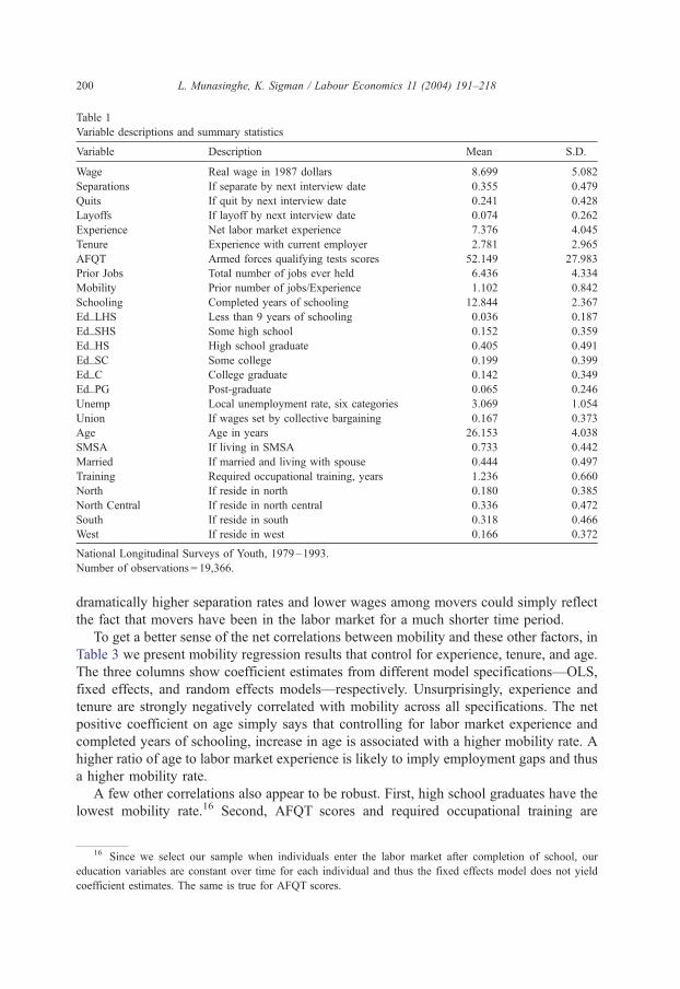
Table 1

Variable descriptions and summary statistics

Variable Description Mean S.D.

Wage Real wage in 1987 dollars 8.699 5.082

Separations If separate by next interview date 0.355 0.479

Quits If quit by next interview date 0.241 0.428

Layoffs If layoff by next interview date 0.074 0.262

Experience Net labor market experience 7.376 4.045

Tenure Experience with current employer 2.781 2.965

AFQT Armed forces qualifying tests scores 52.149 27.983

Prior Jobs Total number of jobs ever held 6.436 4.334

Mobility Prior number of jobs/Experience 1.102 0.842

Schooling Completed years of schooling 12.844 2.367

Ed_LHS Less than 9 years of schooling 0.036 0.187

Ed_SHS Some high school 0.152 0.359

Ed_HS High school graduate 0.405 0.491

Ed_SC Some college 0.199 0.399

Ed_C College graduate 0.142 0.349

Ed_PG Post-graduate 0.065 0.246

Unemp Local unemployment rate, six categories 3.069 1.054

Union If wages set by collective bargaining 0.167 0.373

Age Age in years 26.153 4.038

SMSA If living in SMSA 0.733 0.442

Married If married and living with spouse 0.444 0.497

Training Required occupational training, years 1.236 0.660

North If reside in north 0.180 0.385

North Central If reside in north central 0.336 0.472

South If reside in south 0.318 0.466

West If reside in west 0.166 0.372

National Longitudinal Surveys of Youth, 1979–1993.

Number of observations = 19,366.


dramatically higher separation rates and lower wages among movers could simply reflect

the fact that movers have been in the labor market for a much shorter time period.

To get a better sense of the net correlations between mobility and these other factors, in

Table 3 we present mobility regression results that control for experience, tenure, and age.

The three columns show coefficient estimates from different model specifications—OLS,

fixed effects, and random effects models—respectively. Unsurprisingly, experience and

tenure are strongly negatively correlated with mobility across all specifications. The net

positive coefficient on age simply says that controlling for labor market experience and

completed years of schooling, increase in age is associated with a higher mobility rate. A

higher ratio of age to labor market experience is likely to imply employment gaps and thus

a higher mobility rate.

A few other correlations also appear to be robust. First, high school graduates have the

lowest mobility rate.16 Second, AFQT scores and required occupational training are

16 Since we select our sample when individuals enter the labor market after completion of school, our

education variables are constant over time for each individual and thus the fixed effects model does not yield

coefficient estimates. The same is true for AFQT scores.

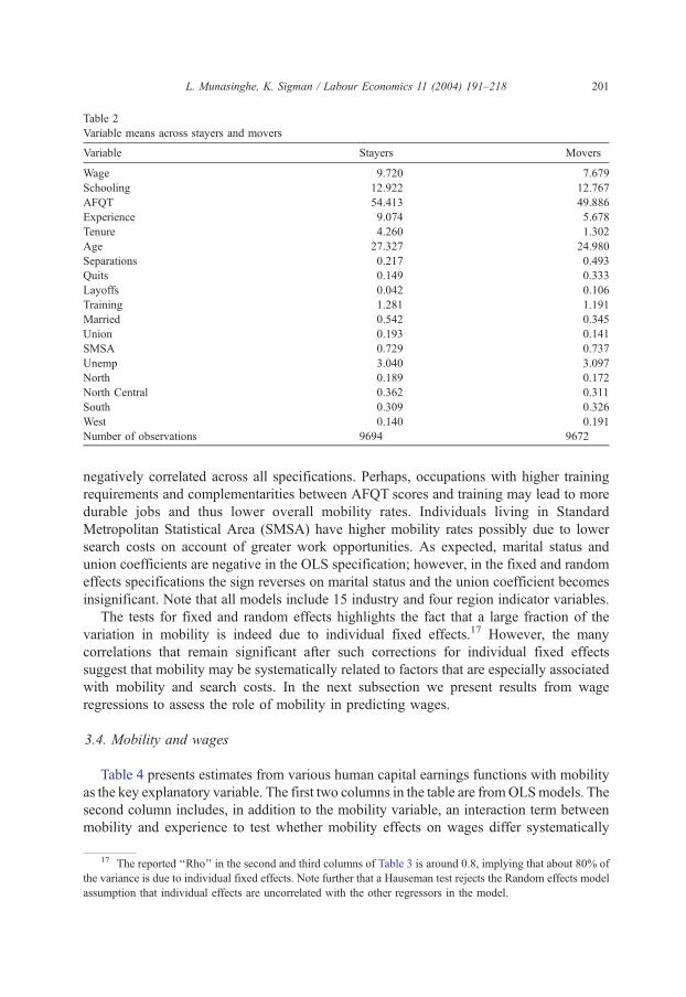
Table 2

Variable means across stayers and movers

Variable Stayers Movers

Wage 9.720 7.679

Schooling 12.922 12.767

AFQT 54.413 49.886

Experience 9.074 5.678

Tenure 4.260 1.302

Age 27.327 24.980

Separations 0.217 0.493

Quits 0.149 0.333

Layoffs 0.042 0.106

Training 1.281 1.191

Married 0.542 0.345

Union 0.193 0.141

SMSA 0.729 0.737

Unemp 3.040 3.097

North 0.189 0.172

North Central 0.362 0.311

South 0.309 0.326

West 0.140 0.191

Number of observations 9694 9672


negatively correlated across all specifications. Perhaps, occupations with higher training

requirements and complementarities between AFQT scores and training may lead to more

durable jobs and thus lower overall mobility rates. Individuals living in Standard

Metropolitan Statistical Area (SMSA) have higher mobility rates possibly due to lower

search costs on account of greater work opportunities. As expected, marital status and

union coefficients are negative in the OLS specification; however, in the fixed and random

effects specifications the sign reverses on marital status and the union coefficient becomes

insignificant. Note that all models include 15 industry and four region indicator variables.

The tests for fixed and random effects highlights the fact that a large fraction of the

variation in mobility is indeed due to individual fixed effects.17 However, the many

correlations that remain significant after such corrections for individual fixed effects

suggest that mobility may be systematically related to factors that are especially associated

with mobility and search costs. In the next subsection we present results from wage

regressions to assess the role of mobility in predicting wages.

3.4. Mobility and wages

Table 4 presents estimates from various human capital earnings functions with mobility

as the key explanatory variable. The first two columns in the table are fromOLSmodels. The

second column includes, in addition to the mobility variable, an interaction term between

mobility and experience to test whether mobility effects on wages differ systematically

17 The reported ‘‘Rho’’ in the second and third columns of Table 3 is around 0.8, implying that about 80% of

the variance is due to individual fixed effects. Note further that a Hauseman test rejects the Random effects model

assumption that individual effects are uncorrelated with the other regressors in the model.

Table 3

Mobility regressions

Variable Coefficient estimates (standard errors)

OLS Fixed effects Random effects

Tenure � 0.214 � 0.099 � 0.107

(0.005) (0.003) (0.003)

Tenure2 0.012 0.006 0.006

(0.0004) (0.0002) (0.0002)

Experience � 0.235 � 0.295 � 0.292

(0.005) (0.006) (0.005)

Experience2 0.007 0.010 0.010

(0.0003) (0.0002) (0.0002)

Age 0.061 0.072 0.072

(0.002) (0.005) (0.004)

Ed_SHS 0.012 0.031

(0.027) (0.067)

Ed_HS � 0.171 � 0.228

(0.026) (0.066)

Ed_SC � 0.073 � 0.041

(0.029) (0.072)

Ed_C � 0.098 � 0.076

(0.031) (0.078)

Ed_PG � 0.090 � 0.0001

(0.034) (0.084)

AFQT � 0.002 � 0.003

(0.0002) (0.001)

Married � 0.038 0.024 0.017

(0.010) (0.007) (0.007)

Unemp � 0.037 � 0.006 � 0.009

(0.005) (0.003) (0.003)

Training � 0.029 � 0.015 � 0.017

(0.007) (0.005) (0.005)

SMSA 0.024 0.031 0.029

(0.011) (0.012) (0.011)

Union � 0.058 � 0.006 � 0.012

(0.013) (0.009) (0.009)

No. of observations 19,366 19,366 19,366

Adjusted R2 0.442 0.382 0.404

Rho 0.837 0.793

Standard errors in parenthesis.


across experience levels. The last two columns show coefficient estimates from fixed effects

and random effects models. The question addressed here is whether the mobility effect in the

OLS specification could be due to some unobserved, time invariant individual effect. Hence

an estimate of a significant mobility effect in the last two specifications would cast doubt on

explanations based on individual fixed effects, such as an inherent individual turnover

propensity or a hobo’s periodic ‘‘itch’’ to move from one job to another job.

Most of the signs of our coefficient estimates are widely established in the literature,

and thus unremarkable. Hence our discussion will focus primarily on the effect of mobility

on wages. In the first column mobility has a strong and significant negative effect on

Table 4

Wage regressions

Variable OLS Fixed effects Random effects

Mobility � 0.027 � 0.010 � 0.019 � 0.016

(0.004) (0.006) (0.006) (0.006)

Mobility*Experience � 0.004 � 0.005 � 0.005

(0.001) (0.001) (0.001)

Tenure 0.050 0.047 0.043 0.045

(0.003) (0.003) (0.002) (0.002)

Tenure2 � 0.003 � 0.003 � 0.003 � 0.003

(0.0002) (0.0002) (0.0002) (0.0002)

Experience 0.024 0.032 0.044 0.040

(0.003) (0.004) (0.003) (0.003)

Experience2 � 0.0003 � 0.001 � 0.001 � 0.001

(0.0002) (0.0002) (0.0002) (0.0002)

Ed_SHS 0.021 0.020 0.032

(0.015) (0.015) (0.027)

Ed_HS 0.075 0.074 0.078

(0.015) (0.015) (0.027)

Ed_SC 0.122 0.122 0.109

(0.016) (0.016) (0.029)

Ed_C 0.233 0.232 0.213

(0.017) (0.017) (0.032)

Ed_PG 0.248 0.247 0.209

(0.019) (0.019) (0.035)

AFQT 0.002 0.002 0.003

(0.0001) (0.0001) (0.0002)

Married 0.086 0.085 0.057 0.065

(0.006) (0.006) (0.006) (0.006)

Union 0.191 0.191 0.138 0.153

(0.007) (0.007) (0.007) (0.007)

Training 0.098 0.098 0.043 0.056

(0.004) (0.004) (0.004) (0.004)

Unemp � 0.019 � 0.019 � 0.021 � 0.022

(0.003) (0.003) (0.003) (0.003)

No. of observation 19,366 19,366 19,366 19,366

Adjusted R2 0.432 0.432 0.336 0.425

Rho 0.584 0.442



wages. Including the interaction of mobility and experience shows that the negative

mobility effect is much stronger among more experienced workers. The fact that these

results are robust across fixed and random effects specifications18—in fact, the negative

18 The F statistic for testing the joint significance of the individual effects in the fixed effects model

specification is highly significant suggesting strong evidence of individual effects in the data. Similarly, the

Lagrange Multiplier test statistic in the context of the random effects model also strongly rejects the OLS

specification with a single constant term. The Hauseman specification test for the random effects model, however,

rejects the assumption that individual effects are uncorrelated with the other regressors in the model. Hence the

data favors the fixed effects model to the random effects model. The key point, however, is that under both these

specifications the mobility effects are fairly similar and highly significant implying that mobility effects persist

despite corrections for individual effects.


mobility effect on wages appears to be slightly stronger under these model specifica-

tions—suggest that the explanation is unlikely to be on account of some unobserved and

time invariant individual effect.19

One important question to ask is why the negative mobility effect on wages might be

stronger among more experienced workers. In the conclusion we conjecture that a possible

explanation may have to do with the optimal sequencing of investments in job search and

firm specific skills over the life cycle. However, from a statistical point of view it is

important to note that our measure of mobility increases in precision with labor market

experience. Since mobility is the ratio of jobs ever held to net labor market experience, this

variable is clearly less noisy for those with longer labor market experience.

3.5. Mobility and job turnover

Tables 5–7 present evidence of the role of mobility in predicting future turnover—i.e.

the likelihood that a worker will change employers between now and the next interview

date, approximately a year later. Table 5 present regression results where the dependent

variable is an overall job separation rate. Tables 6 and 7 duplicate the same analyses for

voluntary and involuntary job separations, respectively. The three columns in each table

represent different model specifications—a linear probability model, a nonlinear logit

model, and a random effects logit model that exploits the panel nature of our data and

hence explicitly accounts for unobserved individual effects.

The remarkable finding is that across all model specifications and different types of

turnover, mobility has a positive effect on future turnover and this positive effect is much

stronger among more experienced workers, as indicated by the positive coefficient of the

interaction between mobility and experience. Of course, the ‘‘hobo syndrome’’ would

predict precisely such a positive correlation between prior mobility and future job

turnover in a simple pooled OLS regression. However, the fact that this effect is stronger

among older workers and the robustness of this positive mobility effect after correcting

for individual fixed effects, suggests, as in the earlier wage analyses, that the relation

between past mobility and future mobility is more systematic than a spurious link due

unobserved heterogeneity. Note further that all the regression analyses control for current

wages. Thus a simple interpretation based on the wage analysis that shows lower wages

among more mobile workers, is clearly also insufficient to explain these turnover

patterns.

Disaggregation of total turnover into quits and layoffs reveal some interesting mobility

patterns. First, tenure and experience always have their negative effect across both quits

and layoffs. The negative effect of marriage on turnover is stronger for quits than it is for

layoffs. High school graduates have lower quit rates but not so noticeably lower layoff

rates. Wages are strongly negatively correlated with quits but positively correlated with

layoffs, as is union status. In a parallel manner, the local unemployment rate is negatively

correlated with quits and positively correlated with layoffs. Thus the insignificant effect of

19 Light and McGarry (1998) also show a very similar result. In their study they not only control for

individual fixed effects but also for job specific effects. Hence they rule out not only individual effects but also

job specific effects as the possible culprit for why stayers earn more than movers.

Table 5

Turnover regressions

Variable Linear

Probability Model

Logit model Random

effects logit

Mobility 0.062 0.198 0.234

(0.008) (0.042) (0.044)

Mobility*Experience 0.007 0.047 0.040

(0.001) (0.008) (0.009)

Log Wages � 0.101 � 0.537 � 0.581

(0.009) (0.048) (0.052)

Tenure � 0.069 � 0.366 � 0.327

(0.003) (0.019) (0.021)

Tenure2 0.004 0.021 0.019

(0.000) (0.002) (0.002)

Experience � 0.011 � 0.065 � 0.060

(0.005) (0.025) (0.026)

Experience2 0.0002 0.001 0.001

(0.0002) (0.001) (0.001)

Ed_SHS � 0.006 � 0.009 0.008

(0.018) (0.093) (0.105)

Ed_HS � 0.050 � 0.223 � 0.235

(0.018) (0.092) (0.104)

Ed_SC � 0.006 0.006 0.012

(0.020) (0.100) (0.113)

Ed_C � 0.026 � 0.087 � 0.091

(0.021) (0.110) (0.124)

Ed_PG 0.015 0.122 0.141

(0.023) (0.122) (0.137)

AFQT � 0.0004 � 0.002 � 0.002

(0.0002) (0.001) (0.001)

Married � 0.029 � 0.160 � 0.071

(0.007) (0.037) (0.040)

Union � 0.017 � 0.100 � 0.111

(0.009) (0.050) (0.052)

Training � 0.013 � 0.062 � 0.066

(0.005) (0.028) (0.029)

Unemp 0.002 0.006 0.002

(0.003) (0.018) (0.019)

No. of observation 19,366



local unemployment rates on overall turnover simply masks these differences across quits

and layoffs. The negative wage effect on overall quits simply reflects the fact that the

negative wage effect on quits dominates the relative weaker positive effect of wages on

layoffs.

3.6. Stochastic dominance of wages of stayers

Table 8 presents some preliminary but novel evidence to address the question of

whether wages of stayers stochastically dominate wages of movers—i.e., whether a higher

Table 6

Quit regressions

Variable Linear

Probability Model

Logit model Random

effects logit

Mobility 0.041 0.100 0.125

(0.007) (0.041) (0.043)


(0.001) (0.008) (0.008)

Log Wages � 0.101 � 0.615 � 0.677

(0.008) (0.052) (0.056)

Tenure � 0.044 � 0.290 � 0.258

(0.003) (0.021) (0.023)

Tenure2 0.003 0.016 0.015

(0.000) (0.002) (0.002)

Experience � 0.003 � 0.035 � 0.029

(0.004) (0.028) (0.028)

Experience2 � 0.0001 � 0.0003 � 0.001

(0.0002) (0.001) (0.001)

Ed_SHS 0.001 0.020 0.041

(0.017) (0.097) (0.109)

Ed_HS � 0.024 � 0.143 � 0.144

(0.017) (0.097) (0.109)

Ed_SC 0.023 0.144 0.168

(0.018) (0.105) (0.118)

Ed_C 0.013 0.103 0.123

(0.020) (0.116) (0.130)

Ed_PG 0.045 0.276 0.308

(0.022) (0.128) (0.143)

AFQT � 0.00002 � 0.0004 � 0.0003

(0.0001) (0.001) (0.001)

Married � 0.014 � 0.099 � 0.106

(0.007) (0.041) (0.043)

Union � 0.043 � 0.361 � 0.373

(0.008) (0.058) (0.061)

Training � 0.009 � 0.043 � 0.046

(0.005) (0.030) (0.031)

Unemp � 0.017 � 0.110 � 0.117

(0.003) (0.019) (0.020)




percent of stayers than of movers have wages above any given wage cutoff level. The

motivation for presenting this evidence is based on an example we present in the next

section where we show that wages of stayers stochastically dominate the wages of movers.

This simple analysis, using the same NLSY data as before, seems to support this

conjecture.

By ‘‘Mob’’ we designate a categorical prior mobility variable that takes values from 1

to 3, representing groups with increasing mobility rates. The ‘‘Exp’’ variable represents

different labor market experience groups in increasing order, and the ‘‘P(W>x)’’ terms

denote the percent of workers who have wages above x, where x represents four (real)

Table 7

Layoff regressions

Variable Linear

Probability Model

Logit model Random

effects logit

Mobility 0.010 � 0.076 � 0.071

(0.005) (0.059) (0.061)


(0.001) (0.012) (0.013)

Log Wages 0.010 0.086 0.094

(0.005) (0.083) (0.085)

Tenure � 0.022 � 0.405 � 0.393

(0.002) (0.039) (0.040)

Tenure2 0.001 0.019 0.018

(0.0002) (0.004) (0.004)

Experience � 0.008 � 0.176 � 0.183

(0.003) (0.044) (0.045)

Experience2 0.0003 0.006 0.006

(0.0001) (0.002) (0.002)

Ed_SHS � 0.003 � 0.034 � 0.036

(0.011) (0.139) (0.149)

Ed_HS � 0.014 � 0.126 � 0.133

(0.011) (0.140) (0.149)

Ed_SC � 0.009 � 0.048 � 0.056

(0.012) (0.156) (0.166)

Ed_C � 0.025 � 0.439 � 0.451

(0.013) (0.187) (0.197)

Ed_PG � 0.011 � 0.071 � 0.070

(0.014) (0.205) (0.216)

AFQT � 0.0001 � 0.003 � 0.003

(0.0001) (0.001) (0.001)

Married � 0.006 � 0.099 � 0.097

(0.004) (0.064) (0.067)

Union 0.034 0.491 0.496

(0.005) (0.074) (0.077)

Training � 0.002 � 0.043 � 0.044

(0.003) (0.048) (0.049)

Unemp 0.015 0.222 0.225

(0.002) (0.028) (0.029)




wage levels starting from 6 and increasing to 24 in intervals of 6.20 Hence the numbers in

the columns represent the percent of workers who have wages above the specified wage

level. The decrease in these numbers for any given experience group, as prior mobility

increases, i.e., going down a column for a given experience group, seems to suggest that

wages of stayers stochastically dominate wages of movers. Not surprisingly, given our

earlier results on the differential impact of mobility on the wages of older and younger

20 We experimented with various other cutoff points with similar results.

Table 8

Stochastic dominance of wages of stayers

Exp Mob Observation P(W>6) P(W>12) P(W>18) P(W>24)

All All 15,965 0.701 0.178 0.032 0.008

All 1 6136 0.821 0.247 0.048 0.010

All 2 7177 0.691 0.164 0.028 0.007

All 3 2652 0.451 0.055 0.009 0.003

1 1 236 0.521 0.102 0.008 0.000

1 2 705 0.590 0.096 0.010 0.004

1 3 514 0.446 0.089 0.008 0.004

2 1 1177 0.764 0.184 0.026 0.003

2 2 2027 0.670 0.166 0.022 0.006

2 3 922 0.436 0.049 0.009 0.002

3 1 1649 0.841 0.278 0.055 0.009

3 2 2037 0.735 0.179 0.037 0.009

3 3 673 0.483 0.048 0.012 0.004

4 1 1614 0.853 0.275 0.071 0.015

4 2 1482 0.742 0.192 0.033 0.008

4 3 355 0.462 0.056 0.008 0.000

5 1 1460 0.859 0.254 0.038 0.014

5 2 926 0.638 0.133 0.024 0.006

5 3 188 0.410 0.021 0.000 0.000

The numbers in the cells represent the percentage of wage observations that are greater than the specified wage

level in the last four columns for different experience and prior mobility categories.


workers, this result of stochastic dominance of stayers’ wages seems especially strong for

the high experience groups.

4. A simple model

In this section we present a simple stochastic model of mobility and wages as a first

step toward rationalizing some of our empirical findings. The motivation here is to provide

a framework to link past mobility to current wages without appealing to any sort of

unobserved individual heterogeneity. In particular, we ask whether human capital and

search considerations alone can help explain why stayers earn more than movers.

4.1. Within-job wage growth, mobility, and wages

Consider a model where workers live for two periods. In each period a worker receives

a wage offer from the same distribution. In a simple search framework, workers change

jobs if and only if they receive a second period wage offer that exceeds the first period

wage. Human capital considerations are introduced to this framework by assuming that

first period wages increase in the second period; in which event, workers change jobs if

and only if the second period wage offer exceeds the first period wage plus the wage

increase. Since the wage offer distribution is the same in both periods the increase in first

period wages is interpreted as a firm specific wage increase.


LetW1 andW2 denote first period and second period wage offers, respectively, assumed

independent random variables from the same wage offer distribution. Further assume that

first period wages increase by c, such that the wage at the end of the first period is simply

W1 + c. If a worker stays in the first job then the second period wage is W1 + c, and if the

worker moves, then the second period wage is W2. The optimal decision criterion is: if

W1 + c>W2, then the worker stays, else the worker moves. In the absence of a first period

wage increase, the order of arrival of offers does not affect the expected value of the

second period wage. That is, by symmetry the expected wage of movers and stayers is the

same:

EðW2 j W2 > W1Þ ¼ EðW1 j W1 > W2Þ ð1Þ

This is a well known result. If, however, the first period wage increases by c then the

expected second period wage of movers is clearly greater than the expected first period

wage of stayers:

EðW2 j W2 > W1 þ cÞ > EðW1 j W1 þ c > W2Þ ð2Þ

In turn, Eq. (2) implies that:

EðW1 þ c j W1 þ c > W2Þ � EðW2 j W2 > W1 þ cÞ < c ð3Þ

The above result says that a comparison of second period wages of stayers and movers will

underestimate the within-job wage increase c (see Topel, 1991). What is more interesting

from the point of view of mobility effects on wages is that the relative second period

wages of stayers and movers cannot be unambiguously signed. The second period wages

of stayers could be either greater or lesser than the second period wages of movers:

EðW1 þ c j W1 þ c > W2ÞaEðW2 j W2 > W1 þ cÞ ð4Þ

The fact that the sign can reverse illustrates that a simple search model with a constant

firm specific wage increase does not lead to a clear-cut prediction between mobility and

wages.21 Whether stayers earn more than movers or the other way around depends on

the exact distribution of wage offers and on the value of c. For example, it can be

demonstrated that if wage offers come from a uniform distribution, then stayers earn

more than movers for all positive values of c (see the first example in Section 4.2

below). This result in turn could explain why stayers are less likely to move in the

future. Note, however, as the counterexample in Section 4.3 illustrates that with another

21 The within-job wage growth parameter c can be viewed more generally as a mobility cost. However, if we

model it as such then the wages of movers will always exceed the wages of stayers since the inequality in Eq. (2)

will now apply not only to the second period wages of movers but also to the second period wages of stayers.

However, since our objective is to rationalize the finding that stayers earn more than movers, we characterize

mobility costs more precisely as a firm-specific wage growth rate because then this parameter of wage growth not

only determines the mobility decision but it also contributes to the second period wages of stayers, and thus

makes it possible for stayers to earn more than movers.


wage offer distribution and for some specific values of c movers can earn more than

stayers.22

Despite the fact that stayers experience wage increases, the reason why they do not

necessarily earn more than movers is due to two other countervailing forces. First, a wage

increase in the first period implies that acceptable second period wage offers must be

relatively high. So movers must receive second period wages that are higher than what

they would have to be if first period wages did not increase. Second, even though the first

period wage increases, lower wage offers in the first period survive because of the wage

increase. It is precisely these considerations that explain why stayers do not necessarily do

better than movers. Therefore, the relative performance of stayers and movers depends on

the distribution of wage offers and on c, the firm specific wage increase. The point is that

this simple rendition of the workhorse theories of labor economics is not silent regarding

the effects of mobility on wages; rather, for the reasons given, it cannot make the

unambiguous prediction that stayers earn more than movers.

4.2. An example: stayers earn more

In this subsection we present a detailed example of wage comparisons between stayers

and movers when the outside wage offer distribution is uniform. We show that stayers do

better than movers for all positive values of wage increases, and do so by stochastically

dominating wages of movers. These results hold for both fixed wage increases and

percentage wage increases. Empirical evidence that support these implications was

presented earlier in Section 3.6.

The uniform density on (a, b) is defined by

f ðxÞ ¼1

b�a; xaða; bÞ

0; otherwise

8<: ð5Þ

and has mean EðW Þ ¼ mba xf ðxÞdx ¼ ðaþ bÞ=2.Given two random variables X and Y, we say that X is stochastically larger than Y,

denoted by Xzst Y, if P(X >x) >P(Y >x) for all x. It is easily seen that such an ordering

implies that E(X)zE(Y). Such an ordering is actually an ordering on the distributions of X

and Y; in particular their tails. Our objective in this section is to show that for the uniform

distribution, stayers always do better than movers. We prove the result in a stochastic

ordering sense which therefore includes the corresponding expected value result (e.g. as in

Eq. (4)).

22 We were interested in obtaining a more general characterization of the role of outside wage offer

distributions in predicting the wages across movers and stayers. For example, we considered whether there might

be some class of distributions for which stayers always did better than movers (or vice versa). In particular, we

tried to use only beta distributions with density on (0, 1) of the form f (x) = xn(1� x)m, but even here we could not

obtain general results that only depend upon the parameters n and m. It appears that these kind of results are

sensitive to more complex properties of distributions.


Given a r.v. X and an event A, by (XjA) we denote a r.v. with the conditional distributionof X given A. Of particular interest to us are the pairs

ðW1 þ c j W1 þ c > W2Þ and ðW2 j W2 > W1 þ cÞ;

ðð1þ aÞW1 j ð1þ aÞW1 > W2Þ and ðW2 j W2 > ð1þ aÞW1Þ:

Proposition 4.1. If wages are distributed as the uniform density on (a, b), then for each

ca(0, b� a), and each aa(0, 1)

ðð1þ aÞW1 j ð1þ aÞW1 > W2Þzst ðW2 j W2 > ð1þ aÞW1Þ

ðW1 þ c j W1 þ c > W2Þzst ðW2 j W2 > W1 þ cÞ:

Proof. We prove only the percentage increase case (1), and do so for a = 0 and b = 1; the

fixed increase case and general 0V a < b being handled similarly. Throughout we use F (x)

to denote the probability that W is less than or equal to x and 1� F̄(x) as the probability

that W is greater than x. Let

P1ðyÞ ¼def

Pðð1þ aÞW1 > y j ð1þ aÞW1 > W2Þ;

P2ðyÞ ¼def

PðW2 > y j W2 > ð1þ aÞW1Þ

Note that when 1V y < 1 + a, P(W2>y) = 0, thus, the result holds trivially for such y and we

need only consider 0V y < 1. Thus we need to show that P1( y)zP2( y), ya(0, 1).

P1ðyÞ ¼ Pðð1þ aÞW1 > y j ð1þ aÞW1 > W2Þ

¼ Pðð1þ aÞW1 > y; ð1þ aÞW1 > W2ÞPðð1þ aÞW1 > W2Þ

¼ N1

D1

;

where N1 and D1 denote the numerator and denominator, respectively. Then conditioning

on W2 = x yields

D1 ¼Z 1

0

F̄x

1þ a

� �f ðxÞdx:

Similarly, conditioning on W2 = xV y and W2 = x>y yields

N1 ¼ F̄y

1þ a

� �FðyÞ þ

Z 1

y

F̄x

1þ a

� �f ðxÞdx:


Thus

P1ðyÞ ¼F̄

y

1þ a

� �FðyÞ þ

Z 1

y

F̄x

1þ a

� �f ðxÞdx

Z 1

0

F̄x

1þ a

� �f ðxÞdx

ð6Þ

On the other hand,

P2ðyÞ ¼ PðW2 > y j W2 > ð1þ aÞW1Þ ¼PðW2 > y;W2 > ð1þ aÞW1Þ

PðW2 > ð1þ aÞW1Þ¼ N2

D2

;

where N2 and D2 denote numerator and denominator. We need only condition on

W1 = x < 1/(1 + a) because P(W2>(1 + a)x) = 0 when xz 1/(1 + a). Doing so yields

D2 ¼Z 1=ð1þaÞ

0

F̄ðð1þ aÞxÞf ðxÞdx:

Similarly, conditioning on W1 = xV y/(1 + a) and W1 = x> y/(1 + a) yields

N2 ¼ F̄ðyÞF y

1þ a

� �þZ 1=ð1þaÞ

y=ð1þaÞF̄ðð1þ aÞxÞf ðxÞdx:

Thus

P2ðyÞ ¼F̄ðyÞF y

1þ a

� �þZ 1=ð1þaÞ

y=ð1þaÞF̄ðð1þ aÞxÞf ðxÞdx

Z 1=ð1þaÞ

0

F̄ðð1þ aÞxÞf ðxÞdxð7Þ

The denominator D1 in Eq. (5) becomes

D ¼Z 1

0

1� x

1þ a

� �dx ¼ ð1þ aÞ�1

Z 1

0

ð1þ a � xÞdx ¼ ð1þ aÞ�1 a þ 1

2

� �:

The numerator N1 becomes

N ¼ ð1þ aÞ�1fð1þ a � yÞyþZ 1

y

ð1þ a � xÞdxg ¼ ð1þ aÞ�1 a þ 1

2� y2

2

� �:

Thus

P1ðyÞ ¼N1

D1

¼ 1� y2

2 a þ 1

2

� � :


Similar computations yield the denominator D2 in Eq. (7) as

D2 ¼ f2ð1þ aÞg�1;

and numerator N2 as

N2 ¼ ð1þ aÞ�1fð1� yÞyþ 1

2ð1� 2yþ y2Þg ¼ f2ð1þ aÞg�1ð1� y2Þ:

Thus

P2ðyÞ ¼N2

D2

¼ 1� y2;

and it is interesting to note that is does not depend on a.Finally,

P1ðyÞ � P2ðyÞ ¼2a

2a þ 1y2z0: 5

4.3. Counterexample: movers earn more

Here we present a counterexample where movers earn more than stayers, illustrating

that in general, the results for the uniform distribution do not extend to all outside wage

offer distributions.

Consider the following wage offer distribution: P(W= 1) = 0.1 and P(W= 10) = 0.9.

Suppose workers sample job offers from this same distribution in both periods. Further

assume, consistent with our model of within-job wage growth, that first period wages

increase by some constant 0 < c < 9. Denote by W1 and W2 the independent random wage

draws from this distribution. Then the expected second period wages of movers and

stayers are given by

EðW2 j W2 > W1 þ cÞ ¼ 10

and

EðW1 þ c j W1 þ c > W2Þ ¼ð0:1Þ2ð1þ cÞ þ ð0:9Þð10þ cÞ

ð0:1Þ2 þ 0:9¼ 9:9011þ c:

respectively. Thus for c < 0.0989 movers earn more than stayers.

4.4. Heterogeneity of wage growth rates

In an earlier paper, Munasinghe (2000) conjectured that heterogeneity of firm specific

wage growth rates among jobs could possibly explain: the negative relationship between

prior mobility and current wages, and the positive relationship between prior mobility and

current turnover. The idea was that high prior mobility could imply both a lower current


job value and, as a result, a higher current turnover rate because prior mobility is a proxy

for wage growth rates of prior jobs. The reason is that the value of low wage-growth jobs

increases less rapidly than the value of high wage-growth jobs (with time on the job). As a

consequence, prior jobs with low wage growth rates lead to higher prior mobility and

relatively low job value.

This idea of heterogeneous wage growth rates is readily incorporated into our two period

model. Stayers do not unambiguously earn more than movers, but they are more likely to

earn higher wages if wage increases are random than if wage increases are constant across

all jobs. The intuition is straightforward. If a worker moves then it is more likely for that

worker to have received a smaller wage increase; and conversely, if a worker stays then it is

more likely that the worker received a higher wage increase. These conclusions follow

because a firm specific wage increase unambiguously reduces the likelihood of moving.

To introduce heterogeneity of wage growth rates, assume that workers in the first period

make draws, independently, from two distributions: first from a wage offer distribution, and

second from a wage growth (increase) distribution. C denotes this random wage increase,

and for simplicity, we assume that the first period wage either increases in the second period

by constant amount c>0 or that it does not, that is, P(C = c) +P(C = 0) = 1. We provide

simple analytics to compare the expected second period wages of stayers with the expected

second period wages of movers. The main objective here is to show that if firm specific

wage growth rates differ among workers or jobs then stayers have a better chance of doing

better than movers than they would otherwise (under constant wage growth). The

randomized wage growth version of Eq. (4) takes the form

EðW1 þ C j W1 þ C > W2ÞaEðW2 j W2 > W1 þ CÞ: ð8Þ

We first present an example in which movers do better under constant wage growth c,

but stayers do better under random wage growth C; it switches. We start with the example

from Section 4.3 with c < 0.0989, so that movers do better.

We now use a random wage growth C with P(C = c) =P(C = 0) = 0.5, and will show that

there are values of c < 0.0989 for which stayers do better. To set up the problem precisely,

note that when C = 0 we need to handle the possibility of a match, W1 =W2. (We could

avoid this by using continuous distributions, but then the computations would be more

involved.) We hereby assume that whenever this happens, the worker will stay or move

with probability 0.5, that is, it is determined by the independent flip of a fair coin. Let T= 1

if the coin lands heads (stay), T= 0 if it lands tails (move). Then by symmetry, given C = 0,

the probability to stay equals one half, the same as to move. Let S denote the event ‘‘stay,’’

and let M denote the event ‘‘move.’’

Proposition 4.2. There exist values of c < 0.0989 such that

EðW1 þ C j SÞ � EðW2 j MÞ > 0 ð9Þ

even though

EðW1 þ c j W1 þ c > W2Þ � EðW2 j W2 > W1 þ cÞ < 0:


To prepare for the proof we first see that each of S and M is the union of three events

describing how each event could occur,

S ¼ fC ¼ c;W1 þ c > W2g [ fC ¼ 0;W1 > W2g [ fC ¼ 0;W1 ¼ W2; T ¼ 1g

M ¼ fC ¼ c;W1 þ c < W2g [ fC ¼ 0;W1 < W2g [ fC ¼ 0;W1 ¼ W2;T ¼ 0g:

Probabilities and conditional probabilities can then be easily computed:

PðSÞ ¼ PðC ¼ cÞ½0:91� þ PðC ¼ 0Þ½0:5�

PðMÞ ¼ PðC ¼ cÞ½0:09� þ PðC ¼ 0Þ½0:5�

p ¼def PðC ¼ 0 j SÞ ¼ PðC ¼ 0Þ½0:5�PðC ¼ cÞ½0:91� þ PðC ¼ 0Þ½0:5�

PðC ¼ c j SÞ ¼ 1� PðC ¼ 0 j SÞ

PðC ¼ c j SÞ ¼ PðC ¼ cÞ½0:91�PðC ¼ cÞ½0:91� þ PðC ¼ 0Þ½0:5�

q ¼def PðC ¼ 0 j MÞ ¼ PðC ¼ 0Þ½0:5�PðC ¼ cÞ½0:09� þ PðC ¼ 0Þ½0:5�

PðC ¼ c j MÞ ¼ 1� PðC ¼ 0 j MÞ

PðC ¼ c j MÞ ¼ PðC ¼ cÞ½0:09�PðC ¼ cÞ½0:09� þ PðC ¼ 0Þ½0:5� :

For example,

PðC ¼ c;W1 þ c > W2Þ ¼ PðC ¼ cÞ½PðW1 ¼ 1;W2 ¼ 1Þ þ PðW1 ¼ 10Þ�¼ PðC ¼ cÞ½ð0:1Þ2 þ 0:9� ¼ PðC ¼ cÞ½0:91�;

and

PðC ¼ 0;W1 > W2Þ þ PðC ¼ 0;W1 ¼ W2; T ¼ 1Þ ¼ PðC ¼ 0Þ0:5;

by symmetry.


Proof . We can express each of the desired expectations as weighted sums,

EðW1 þ C j SÞ ¼ pEðW1 j S;C ¼ 0Þ þ ð1� pÞEðW1 þ c j S;C ¼ cÞ

EðW2 j MÞ ¼ qEðW2 j M ;C ¼ 0Þ þ ð1� qÞEðW2 j M ;C ¼ cÞ:

By symmetry E(W1jS, C = 0) =E(W2jM, C = 0) =P(W1>W2)+(0.5)P(W1 =W2) = 9.91 so

the difference in Eq. (9) is given by

ðp� qÞð9:91Þ þ ð1� pÞEðW1 þ c j S;C ¼ cÞ � ð1� qÞEðW2 j M ;C ¼ cÞ:

Each of the expected values is easily computed directly yielding the difference as

EðW1 þ C j SÞ � EðW2 j MÞ ¼ ðp� qÞð9:91Þ þ ð1� pÞð9:9011þ cÞ � ð1� qÞ10¼ ð1� pÞðc� 0:0089Þ � ð1� qÞð0:09Þ;

where we have used the basic fact that p+(1� p) = 1 and q+(1� p) = 1.

It is at this point that we plug in P (C = 0) =P(C = c) = 0.5 into the formulas for p and q

getting 1� p = 0.6450, 1� q = 0.1525 so that E(W1 +CjS)�E(W2jM) = 0.645c� 0.0195,

and we see that for c>0.0323, the difference is strictly positive. 5

We now present another general result and we assume for simplicity that wage

distributions are continuous (to avoid ties):

Proposition 4.3 . If stayers do better than movers under constant c wage growth, then they

continue doing better under random wage growth C; E(W1+CjW1+C>W2)>E(W2jW2>

W1+C) if E(W1+ cjW1+ c>W2)>E(W2jW2>W1+ c).

Proof . Using the assumption that E(W1 + cjW1 + c>W2)>E(W2jW2>W1 + c) we can express

the difference d =E(W1 +CjW1 +C >W2)�E(W2jW2>W1 +C) as

d ¼ ðp� qÞEðW1 j W1 > W2Þ þ ð1� pÞEðW1 þ c j W1 þ c > W2Þ� ð1� qÞEðW2 j W2 > W1 þ cÞ > ðp� qÞEðW1 j W1 > W2Þ þ ðð1� pÞ� ð1� qÞÞEðW2 j W2 > W1 þ cÞz½ðp� qÞ þ ðð1� pÞ � ð1� qÞÞ�� EðW1 j W1 > W2Þ ¼ 0;

where, in the z line we have used the fact that E(W2jW2>W1 + c)zE(W2jW2>W1) =E(W1jW1>W2) and that (1� p)� (1� q)z 0 (since 1� p =P(C = 1jS)z 1� q =P(C = 1jM)).

Thus d>0 as was to be shown. 5

This section clearly shows that heterogeneity of wage growth rates among jobs makes it

more likely that stayers earn more than movers. As a result, the size of within-job wage


growth may be less relevant than the heterogeneity of such wage growth rates. Despite the

mechanical framework adopted here, the key point of these analytics is to show that

mobility effects on wages may be generated without appealing any sort of individual fixed

effect.23 Although it is beyond the scope of this paper, perhaps a more realistic equilibrium

model of mobility and wages, where the optimization of both workers and firms are

explicitly considered, can generate results consistent with our findings about the net effects

of mobility on wages and turnover.

5. Conclusion

A possible extension to this work is to explicitly model the differential effects of prior

mobility across more and less experienced workers. It is reasonable to suppose that

workers search for goodmatches in the early part of their careers (job search process), and

then, subsequent to finding a good match, workers invest in firm specific human capital.

This sequencing of search and investment processes can be derived from ideas already

present in the literature. For example, the basic intuition in Jovanovic (1979b) is that good

matches create incentives to invest in firm specific human capital because good matches

are more durable. Since good matches take time to find, young workers are more likely to

be involved in search, while older workers (consequent to finding a good match) are more

likely to be involved in firm specific investments. A similar idea can be found in Antel

(1986), where he argues that specific training and search represent mutually exclusive

human capital investments because specific skills cannot be transferred between jobs and

because search and training are costly; as a consequence, ‘‘at a given time, workers will

choose between more training specific to their current job or opt for further search leading

to some more remunerative employment’’ (Antel, 1986, p. 477). It seems more likely that

young workers will opt to search and that older workers will opt to invest in job specific

training. These ideas could be extended to study the optimal life cycle sequence of search

and specific investments with ramifications for differential effects of prior mobility on

wages and turnover of older and young workers.

We also conjecture that stayers will tend to earn more than movers over time. In the

limit where the current wage of stayers (presumably due to wage growth) is higher than the

best outside offer (assuming a distribution with an upper bound), it is easy to understand

why stayers would earn more than movers irrespective of the specifics of the outside wage

offer distributions. Such a result would further support the findings of differential impact

of prior mobility on wages and turnover of older and younger workers.

Finally, it is important to ask whether the results for the uniform distribution hold for

other distributions. The empirical results imply that this is so for the ‘‘real’’ wage offer

distribution. But of course we do not know what that distribution is: recorded wage data

are not from the underlying wage offer distribution; they are conditional distributions

from it.

23 Note that heterogeneity of wage growth rates is not a fixed individual effect. In the current formulation it

can be viewed as a parameter specific to each worker-firm pair. For a more detailed discussion see Munasinghe

(2001).


Acknowledgements

We thank Cynthia Howells, Tackseung Jun, Brendan O’Flaherty, Nachum Sicherman,

and Sanjay Tikku for helpful comments, and Erin Chan for conscientious research

assistance. We also thank our Editor Dan Black and the referees for their detailed and

many excellent comments.

References

Abowd, J.M., Kramarz, F., Margolis, D., 1999. High wage workers and high wage firms. Econometrica 67 (2),

251–333.

Abraham, K., Farber, H., 1987. Job duration, seniority, and earnings. American Economic Review 77, 278–297.

Altonji, J., Shakotko, R., 1987. Do wages rise with job seniority. Review of Economic Studies 54, 437–459.

Altonji, J., Williams, N., 1997. Do Wages Rise with Job Seniority? A Reassessment. NBER, Working Paper

#6010.

Antel, J.J., 1986. Human capital investment specialization and the wage effects of voluntary labor mobility.

Review of Economics and Statistics 68, 477–483.

Barron, J., Black, D., Loewenstein, M., 1993. Gender differences in training, capital, and wages. Journal of

Human Resources 28, 343–364.

Bartel, A., Borjas, G., 1981. In: Rosen, S. (Ed.), Wage Growth and Job Turnover: An Empirical Analysis. Studies

in Labor Markets. University of Chicago Press for the NBER, Chicago, IL.

Becker, G., 1975. Human Capital, 2nd ed. University of Chicago Press for the NBER, Chicago, IL.

Black, D., Loewenstein, M., 1991. Self-enforcing labor contracts with costly mobility. Research in Labor

Economics 12, 63–68.

Blumen, I., Kogan, M., McCarthy, P., 1955. The Industrial Mobility of Labor as a Probability Process. Cornell

Univ. Press, Ithaca, NY.

Burdett, K., 1978. Theory of employee search: quit rates. American Economic Review 68, 212–220.

Carrington, W., 1993. Wage losses for displaced workers: is it really the firm that matters? Journal of Human

Resources 28 (3), 435–462.

Ghiselli, E.E., 1974. Some perspectives for industrial psychology. American Psychologist, 80–87 (Feb.).

Greene, W.H., 2003. Econometric analysis, 5th ed. Prentice Hall, New Jersey.

Jovanovic, B., 1979a. Job matching and the theory of turnover. Journal of Political Economy 87 (5), 972–990.

Jovanovic, B., 1979b. Firm-specific capital and turnover. Journal of Political Economy 87 (6), 1246–1260.

Judge, T., Watanabe, S., 1995. Is the past prologue: a test of Ghiselli’s hobo syndrome. Journal of Management

21 (2), 211–229.

Kuhn, P., 1993. Demographic groups and personnel policy. Labour Economics 1, 49–70.

Light, A., McGarry, K., 1998. Job change patterns and the wages of young men. Review of Economics and

Statistics 80 (2), 276–286.

Mincer, J., 1986. Wage changes in job changes. Research in Labor Economics 8 (A), 171–197.

Mincer, J., 1988. Job Training, Wage Growth, and Labor Turnover. NBER Working paper.

Mincer, J., Jovanovic, B., 1981. In: Rosen, S. (Ed.), Labor Mobility and Wages. Studies in Labor Markets.

University of Chicago Press for the NBER, Chicago, IL, pp. 21–63.

Munasinghe, L., 2000. Wage growth and the theory of turnover. Journal of Labor Economics 18 (2), 204–220.

Munasinghe, L., 2001. A Theory of Wage and Turnover Dynamics, Working Paper 02-01, Barnard College,

Columbia University, New York, NY.

Neal, D., 1995. Industry-specific human capital: evidence from displaced workers. Journal of Labor Economics

13 (4), 653–677.

Topel, R.H., 1991. Specific capital, mobility, and wages: wages rise with job seniority. Journal of Political

Economy 9 (1), 145–176.

Weiss, A., Landau, H., 1984. Mobility and wages. Economics Letters 15, 97–102.

a hobo syndrome? mobility, wages, and job turnoverlm25/le-2004.pdfa hobo syndrome? mobility, wages,...

Documents