A Hybrid Approach to Functional Dependency Discovery

Thorsten PapenbrockHasso Plattner Institute (HPI)

14482 Potsdam, Germanythorsten.papenbrock@hpi.de

Felix NaumannHasso Plattner Institute (HPI)

14482 Potsdam, Germanyfelix.naumann@hpi.de

ABSTRACTFunctional dependencies are structural metadata that canbe used for schema normalization, data integration, datacleansing, and many other data management tasks. Despitetheir importance, the functional dependencies of a specificdataset are usually unknown and almost impossible to dis-cover manually. For this reason, database research has pro-posed various algorithms for functional dependency discov-ery. None, however, are able to process datasets of typicalreal-world size, e.g., datasets with more than 50 attributesand a million records.

We present a hybrid discovery algorithm called HyFD,which combines fast approximation techniques with efficientvalidation techniques in order to find all minimal functionaldependencies in a given dataset. While operating on com-pact data structures, HyFD not only outperforms all exist-ing approaches, it also scales to much larger datasets.

1. FUNCTIONAL DEPENDENCIESA functional dependency (FD) written as X → A ex-

presses that all pairs of records with same values in at-tribute combination X must also have same values in at-tribute A [6]. The values in A functionally depend on thevalues in X. Consequently, keys in relational datasets ex-press functional dependencies, because they uniquely deter-mine all other attributes. Functional dependencies also arisenaturally from real-world facts that a dataset describes. Inaddress datasets, for instance, a person’s firstname mightdetermine the gender attribute, the zipcode might determinecity, and birthdate should determine age.

The most important use for functional dependencies isschema normalization [5]. Normalization processes system-atically decompose relations with their functional dependen-cies to reduce data redundancy. But functional dependenciesalso support further data management tasks, such as queryoptimization [22], data integration [17], data cleansing [3],and data translation [4]. Although we find many such usecases, functional dependencies are almost never specified as

Permission to make digital or hard copies of all or part of this work for personal orclassroom use is granted without fee provided that copies are not made or distributedfor profit or commercial advantage and that copies bear this notice and the full cita-tion on the first page. Copyrights for components of this work owned by others thanACM must be honored. Abstracting with credit is permitted. To copy otherwise, or re-publish, to post on servers or to redistribute to lists, requires prior specific permissionand/or a fee. Request permissions from permissions@acm.org.

SIGMOD’16, June 26-July 01, 2016, San Francisco, CA, USAc© 2016 ACM. ISBN 978-1-4503-3531-7/16/06. . . $15.00

DOI: http://dx.doi.org/10.1145/2882903.2915203

concrete metadata. One reason is that they depend not onlyon a schema but also on a concrete relational instance. Forexample, child → teacher might hold for kindergarten chil-dren, but it does not hold for high-school children. Conse-quently, functional dependencies also change over time whendata is extended, altered, or merged with other datasets.Therefore, discovery algorithms are needed that reveal allfunctional dependencies of a given dataset.

Due to the importance of functional dependencies, manydiscovery algorithms have already been proposed. Unfor-tunately, none of them is able to process datasets of real-world size, i.e., datasets with more than 50 columns anda million rows, as a recent study showed [20]. Becausethe need for normalization, cleansing, and query optimiza-tion increases with growing dataset sizes, larger datasets arethose for which functional dependencies are most urgentlyneeded. The reason why current algorithms fail on largerdatasets is that they optimize for either many records ormany attributes. This is a problem, because the discovery offunctional dependencies is by nature quadratic in the num-ber of records n and exponential in the number attributesm. More specifically, it is in O(n2(m

2)22m) as shown by Liu

et al. [15]. Therefore, any truly scalable algorithm must beable to cope with both large schemata and many rows.

To approach such datasets, we propose a novel hybridalgorithm called HyFD, which combines row- and column-efficient discovery techniques: In a first phase, HyFD ex-tracts a small subset of records from the input data and cal-culates the FDs of this non-random sample. Because onlya subset of records is used in this phase, it performs par-ticularly column-efficient. The result is a set of FDs thatare either valid or almost valid with respect to the completeinput dataset. In a second phase, HyFD validates the dis-covered FDs on the entire dataset and refines such FDs thatdo not yet hold. This phase is row-efficient, because it usesthe previously discovered FDs to effectively prune the searchspace. If the validation becomes inefficient, HyFD is able toswitch back into the first phase and continue there with allresults discovered so far. This alternating, two-phased dis-covery strategy clearly outperforms all existing algorithmsin terms of runtime and scalability, while still discovering allminimal FDs. In detail, our contributions are the following:

(1) FD discovery. We introduce HyFD, a hybrid FD dis-covery algorithm that is faster and able to handle muchlarger datasets than state-of-the-art algorithms.

(2) Focused sampling. We present sampling techniques thatleverage the advantages of dependency induction algorithmswhile, at the same time, requiring far fewer comparisons.

(3) Direct validation. We contribute an efficient validationtechnique that leverages the advantages of lattice traversalalgorithms with minimal memory consumption.

(4) Robust scaling. We propose a best-effort strategy thatdynamically limits the size of resulting FDs if these wouldotherwise exhaust the available memory capacities.

(5) Exhaustive evaluation. We evaluate our algorithm onmore than 20 real-world datasets and compare it to sevenstate-of-the-art FD discovery algorithms.

In the following, Section 2 discusses related work. Then,Section 3 provides the theoretical foundations for our dis-covery strategy and Section 4 an overview on our algorithmHyFD. Sections 5, 6, 7, and 8 describe the different com-ponents of HyFD in more detail. Section 10 evaluates ouralgorithm and compares it against seven algorithms fromrelated work. We then conclude in Section 11.

2. RELATED WORKThe evaluating work of [20] compared the seven most

popular algorithms for functional dependency discovery anddemonstrated their individual strengths and weaknesses.Some effort has also been spent on the discovery of approxi-mate [12] and conditional [3,7] functional dependencies, butthose approaches are orthogonal to our research: We aim todiscover all minimal functional dependencies without anyrestrictions or relaxations. Parallel and distributed depen-dency discovery systems, such as [10] and [14], form anotherorthogonal branch of research. They rely on massive par-allelization rather than efficient pruning to cope with thediscovery problem. We focus on more sophisticated searchtechniques and show that these can still be parallelized ac-cordingly. In the following, we briefly summarize currentstate-of-the-art in non-distributed FD discovery.

Lattice traversal algorithms: The algorithms Tane [12],Fun [18], Fd Mine [25], and Dfd [1] conceptually arrangeall possible FD candidates in a powerset lattice of attributecombinations and then traverse this lattice. The first threealgorithms search through the candidate lattice level-wisebottom-up using the apriori-gen candidate generation [2],whereas Dfd applies a depth-first random walk. Latticetraversal algorithms in general make intensive use of prun-ing rules and their candidate validation is based on strippedpartitions (also called position list indices). They have beenshown to perform well on long datasets, i.e., datasets withmany records, but due to their candidate-driven search strat-egy, they scale poorly with the number of columns in the in-put dataset. In this paper, we adopt the pruning rules andthe position list index data structure from these algorithmsfor the validation of functional dependencies.

Difference- and agree-set algorithms: The algorithmsDep-Miner [16] and FastFDs [24] analyze a dataset for setsof attributes that agree on the values in certain tuple pairs.These so-called agree-sets are transformed into difference-sets from which all valid FDs can be derived. This dis-covery strategy scales better with the number of attributesthan lattice traversal strategies, because FD candidates aregenerated only from concrete observations rather than be-ing generated systematically. The required maximizationand minimization of agree- and difference-sets respectively,however, reduces this advantage significantly. With regardto the number of records, Dep-Miner and FastFDs scale

much worse than the previous algorithms, because they needto compare all pairs of records. Our approach also comparesrecords pair-wise, but we choose these comparisons carefully.

Dependency induction algorithms: The Fdep [9] algo-rithm also compares all records pair-wise to find all invalidfunctional dependencies. This set is called negative coverand is stored in a prefix tree. In contrast to Dep-Minerand FastFDs, Fdep translates this negative cover into theset of valid functional dependencies, i.e., the positive cover,not by forming complements but by successive specializa-tion: The positive cover initially assumes that each attributefunctionally determines all other attributes; these functionaldependencies are then refined with every single non-FD inthe negative cover. Apart from the fact that the pair-wisecomparisons do not scale with the number of records in theinput dataset, this discovery strategy has proven to scalewell with the number of attributes. For this reason, we fol-low a similar approach during the induction of functionaldependency candidates. However, we compress records be-fore comparison, store the negative cover in a more efficientdata structure, and optimize the specialization process.

The evaluation section of this paper provides a comparisonof our approach with all mentioned related work.

3. HYBRID FD DISCOVERYWe begin this section by formally defining functional de-

pendencies (FDs). We then discuss sampling-based FD dis-covery and our hybrid discovery approach.

Preliminaries. Our definition of a functional dependencyfollows [23]: A functional dependency (FD) written as X →A is a statement over a relational schema R, where X ⊆ Rand A ∈ R. The FD is valid for an instance r of R, iff for allpairs of tuples t1, t2 ∈ r the following is true: if t1[B] = t2[B]for all B ∈ X, then t1[A] = t2[A]. In other words, thevalues in X functionally determine the values in A. We callthe determinant X the FD’s left hand side (Lhs), and thedependent A the FD’s right hand side (Rhs). Moreover, anFD X → A is a generalization of another FD Y → A ifX ⊂ Y and it is a specialization if X ⊃ Y . The FD X → Ais non-trivial if A /∈ X and it is minimal if no B exists suchthat X\B → A is a valid FD, i.e., if no valid generalizationexists. To discover all FDs in a given relational instance r,it suffices to discover all minimal, non-trivial FDs, becauseall Lhs-subsets are non-dependencies and all Lhs-supersetsare dependencies by logical inference.

The discovery of all minimal, non-trivial FDs can best bemodeled as a graph search problem: The graph is a powersetlattice of attribute combinations and an edge between thenodes X and XA represents the FD candidate X → A.Figure 1 depicts an example lattice and its FDs and non-FDs. In all such lattices, FDs are located in the upper partof the lattice; non-FDs are located at the bottom. A virtualborder separates the FDs and non-FDs. All minimal FDs,which we aim to discover, reside on this virtual border line.

Sampling-based FD discovery. For a relational instancer, a sample r′ of r contains only a subset of records r′ ⊂ r.Because r′ is smaller than r, discovering all minimal FDson r′ is expected to be cheaper than discovering all minimalFDs on r (with any FD discovery algorithm). The resultingr′-FDs can, then, be valid or invalid in r, but they exhibitthree properties that are important for our hybrid algorithm:

minimal FDs non-FDs

A B C D E

AB AC AD AE BC BD BE CD CE DE

ABC ABD ABE ACD ACE ADE BCD BCE BDE CDE

ABCD ABCE ABDE ACDE BCDE

ABCDE

non-minimal FDs

Ø

Figure 1: FD discovery in a power set lattice.

(1) Completeness: The set of r′-FDs implies the set of r-FDs, i.e., we find an X ′ → A in r′ for each valid X → A in rwith X ′ ⊆ X. Hence, all X → A are also valid in r′ and thesampling result is complete. To prove this, assume X → A isvalid in r but invalid in r′. Then r′ must invalidate X → Awith two records that do not exist in r. So it is r′ 6⊂ r, whichcontradicts r′ ⊂ r.(2) Minimality: If a minimal r′-FD is valid on the entireinstance r, then the FD must also be minimal in r. Thismeans that the sampling cannot produce non-minimal orincomplete results. In other words, a functional dependencycannot be valid in r but invalid in r′. This property is easilyproven: If X → A is invalid in r′, then r′ contains tworecords with same X values but different A values. Becauser′ ⊂ r, the same records must also exist in r. Therefore,X → A must be invalid in r as well.

(3) Proximity: If a minimal r′-FD is invalid on the entireinstance r, then the r′-FD is still close to specializationsthat are valid in r. In other words, r′-FDs are always lo-cated closer to the virtual border, which holds the true r-FDs, than the FDs at the bottom of the lattice. Therefore,any sampling-based FD discovery algorithm approximatesthe real FDs. The distance between r′-FDs and r-FDs stilldepends on the sampling algorithm and the entire data.

In summary, a sampling-based FD discovery algorithmcalculates a set of r′-FDs that are either r-FDs or possiblyclose generalizations of r-FDs. In terms of Figure 1, theresult of the sampling is a subset of solid lines.

The hybrid approach. Recently, the authors of [20] madethe observation that current FD discovery algorithms ei-ther scale well with the number of records (e.g., Dfd) orthey scale well with the number of attributes (e.g., Fdep).None of the algorithms, however, addresses both dimen-sions equally well. Therefore, we propose a hybrid algo-rithm that combines column-efficient FD induction tech-niques with row-efficient FD search techniques in two phases.

In Phase 1, the algorithm uses column-efficient FD induc-tion techniques. Because these are sensitive to the numberof rows, we process only a small sample of the input. Theidea is to produce with low effort a set of FD candidatesthat are according to property (3) proximity close to thereal FDs. To achieve this, we propose focused samplingtechniques that let the algorithm select samples with a pos-sibly large impact on the result’s precision. Due to samplingproperties (1) completeness and (2) minimality, these tech-niques cannot produce non-minimal or incomplete results.

In Phase 2, the algorithm uses row-efficient FD searchtechniques to validate the FD candidates given by Phase 1.

Because the FD candidates and their specializations repre-sent only a small subset of the search space, the numberof columns in the input dataset has a much smaller impacton the row-efficient FD search techniques. Furthermore, theFD candidates should be valid FDs or close to valid special-izations due to sampling property (3) proximity. The task ofthe second phase is, hence, to check all FD candidates andto find valid specializations if a candidate is invalid.

Although the two phases match perfectly, finding an ap-propriate, dataset-independent criterion for when to switchfrom Phase 1 into Phase 2 is difficult. If we switch too earlyinto Phase 2, the FD candidates approximate the real FDsonly poorly and the search space becomes large; if we remaintoo long in Phase 1, we might end up analyzing the entiredataset with only column-efficient FD induction techniques,which is very expensive on many rows. For this reason, wepropose to switch between the two phases back and forthwhenever the currently running strategy becomes inefficient.

For Phase 1, we track the sampling efficiency, which is de-fined as the number of new observations per comparison. Ifthis efficiency falls below an optimistic threshold, the algo-rithm switches into Phase 2. In Phase 2, we then track thevalidation efficiency, which is the number of discovered validFDs per validation. Again, if this efficiency drops below agiven threshold, the validation process can be consideredinefficient and we switch back into Phase 1. In this case,the previous sampling threshold was too optimistic, so thealgorithm dynamically increases it.

When switching back and forth between the two phases,the algorithm can share insights between the different strate-gies: The validation phase obviously profits from the FDcandidates produced by the sampling phase; the samplingphase, in turn, profits from the validation phase, becausethe validation hints on interesting tuples that already inval-idated some FD candidates. The hybrid FD discovery ter-minates when Phase 2 finally validated all FD candidates.We typically observe three to eight switches from Phase 2back into Phase 1 until the algorithm finds the complete setof minimal functional dependencies. This result is correct,complete, and minimal, because Phase 1 is complete andminimal, as we have shown, and Phase 2 finally releases acorrect, complete, and minimal result as shown by [12].

4. THE HYFD ALGORITHMWe implemented the hybrid FD discovery approach as

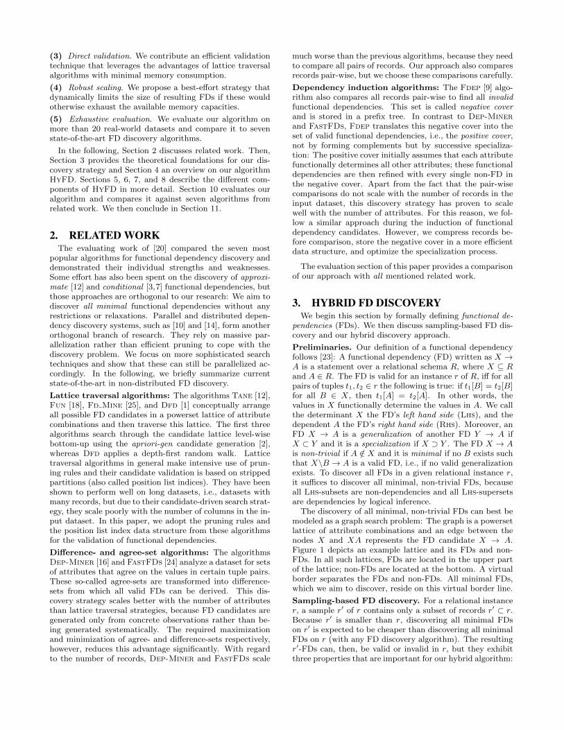
the HyFD algorithm. Figure 2 gives an overview of HyFDshowing its components and the control flow between them.In the following, we briefly introduce each component andtheir tasks in the FD discovery process. Each component islater explained in detail in their respective sections. Notethat the Sampler and the Inductor component together im-plement Phase 1 and the Validator component implementsPhase 2.

(1) Preprocessor. To discover functional dependencies, wemust know the positions of same values for each attribute,because same values in an FD’s Lhs can make it invalidif the according Rhs values differ. The values itself, how-ever, must not be known. Therefore, HyFD’s Preprocessorcomponent first transforms the records of a given datasetinto compact position list indexes (Pli). For performancereasons, the component also pre-calculates the inverse ofthis index, which is later used in the validation step. Be-

HyFD

records

plis, pliRecords

non-FDs

candidate-FDs

FDs

plis, pliRecords

comparisonSuggestions

results

FD

Validator

dataset

FD Candidate

Inductor

Record Pair

Sampler

Memory

Guardian

Data

Preprocessor

Figure 2: Overview of HyFD and its components.

cause HyFD uses sampling to combine row- with column-efficient discovery techniques, it still needs to access the in-put dataset’s records. For this purpose, the Preprocessor

compresses the records using the Plis as dictionaries.

(2) Sampler. The Sampler component implements the firstpart of a column-efficient FD induction technique: It startsthe FD discovery by checking the compressed records forFD-violations. An FD-violation is a pair of two records thatmatch in one or more attribute values. From such recordpairs, the algorithm infers that the matching attributescannot functionally determine any of the non-matching at-tributes. Hence, they indicate non-valid FDs or short non-FDs. The schema R(A,B,C), for instance, could hold thetwo records r1(1, 2, 3) and r2(1, 4, 5). Because the A-valuesmatch and the B- and C-values differ, A 6→ B and A 6→ Care two non-FDs in R. Finding all these non-FDs requiresto systematically match all records pair-wise. Because thisquadratic complexity does not scale in practice, the Sampler

carefully selects only a subset of record pairs, namely thosethat indicate possibly many FD-violations. For the selectionof record pairs, the component uses a deterministic, focusedsampling technique that we call cluster windowing.

(3) Inductor. The Inductor component implements thesecond part of the column-efficient FD induction technique:From the Sampler component, it receives a rich set of non-FDs that must be converted into FD-candidates. An FD-candidate is an FD that is minimal and valid with respectto the chosen sample – whether a candidate is actuallyvalid on the entire dataset is determined in Phase 2. Theconversion algorithm is similar to the Fdep algorithm [9]:We first assume that the empty set functionally determinesall attributes; then, we successively specialize this assump-tion with every known non-FD. Recall the example schemaR(A,B,C) and its known non-FD A 6→ B. Initially, we de-fine our result to be ∅ → ABC, which is a short notation forthe FDs ∅ → A, ∅ → B, and ∅ → C. Because A 6→ B, theFD ∅ → B, which is a generalization of our known non-FD,must be invalid as well. Therefore, we remove it and addall valid, minimal, non-trivial specializations. Because thisis only C → B, our new result set is ∅ → AC and C → B.To execute the specialization process efficiently, the Induc-

tor component maintains the valid FDs in a prefix tree thatallows for fast generalization look-ups. If the Inductor iscalled again, it can continue specializing the FDs that it al-ready knows, so it does not start with an empty prefix tree.

(4) Validator. The Validator component implements arow-efficient FD search technique: It takes the candidate-FDs from the Inductor and validates them against the entiredataset, which is given as a set of Plis from the Preproces-

sor. When modeling the FD search space as a powersetlattice, the given candidate-FDs approximate the final FDsfrom below, i.e., a candidate-FD is either a valid FD or a gen-eralization of a valid FD. Therefore, the Validator checksthe candidate-FDs level-wise bottom-up: Whenever the al-gorithm finds an invalid FD, it exchanges this FD with allits minimal, non-trivial specializations using common prun-ing rules for lattice traversal algorithms [12]. If previouscalculations yielded a good approximation of the valid FDs,only few FD candidates need to be specialized; otherwise,the number of invalid FDs increases rapidly from level tolevel and the Validator switches back to Sampler. The FDvalidations themselves build upon direct refinement checksand avoid the costly hierarchical Pli intersections that aretypical in all current lattice traversal algorithms. In the end,the Validator outputs all minimal, non-trivial FDs for thegiven input dataset.

(5) Guardian. FD result sets can grow exponentially withthe number of attributes in the input relation. For this rea-son, discovering complete result sets can sooner or later ex-haust any memory-limit, regardless of how compact inter-mediate data structures, such as Plis or results, are stored.Therefore, a robust algorithm must prune the results insome reasonable way, if memory threatens to be exhausted.This is the task of HyFD’s Guardian component: When-ever the prefix tree, which contains the valid FDs, grows,the Guardian checks the current memory consumption andprunes the FD tree, if necessary. The idea is to give upFDs with largest left-hand-sides, because these FDs mostlyhold accidentally in a given instance but not semantically inthe according schema. Overall, however, the Guardian is anoptional component in the HyFD algorithm and does notcontribute in the discovery process itself. Our overarchinggoal remains to find the complete set of minimal FDs.

5. PREPROCESSINGThe Preprocessor is responsible for transforming the

input data into two compact data structures: plis andpliRecords. The first data structure plis is an array of po-sition list indexes (Pli). In the literature, these Plis arealso known as stripped partitions [8, 12]. A Pli, denotedby πX , groups tuples into equivalence classes by their val-ues of attribute set X. Thereby, two tuples t1 and t2 ofan attribute set X belong to the same equivalence class if∀A ∈ X : t1[A] = t2[A]. These equivalence classes are alsocalled clusters, because they cluster records by same values.For compression, a Pli does not store clusters with only asingle entry, because tuples that do not occur in any clusterof πX can be inferred to be unique in X. Consider, for exam-ple, the relation Class(Teacher, Subject) and its tuples (Brown,

Math), (Walker, Math), (Brown, English), (Miller, English), and(Brown, Math). Then, π{Teacher} = {{1, 3, 5}}, π{Subject} ={{1, 2, 5}, {3, 4}}, and π{Teacher,Subject} = {{1, 5}}. SuchPlis can efficiently be implemented as sets of record ID sets,which we wrap in Pli objects.

To check a functional dependency X → A using only Plis,we can test if every cluster in πX is a subset of some clusterof πA. If this holds true, then all tuples with same values in

X have also same values in A, which is the definition of anFD. This check is called refinement (see Section 8) and wasfirst introduced in [12].

Algorithm 1 shows the Preprocessor component and thetwo data structures it produces: The already discussed plisand a Pli-compressed representation of all records, whichwe call pliRecords. For their creation, the algorithm firstdetermines the number of input records numRecs and thenumber of attributes numAttrs (Lines 1 and 2). Then, itbuilds the plis array – one π for each attribute. This is doneby hashing each value to a list of record IDs and then simplycollecting these lists in a Pli object (Line 4). When created,the Preprocessor sorts the array of Plis in descending orderby the number of clusters (including clusters of size one,whose number is implicitly known). This sorting improvesthe FD-candidate validations of the Validator component,which we discuss in Section 8.

Algorithm 1: Data Preprocessing

Data: recordsResult: plis, invertedPlis, pliRecords

numRecs ← |records|;1

numAttrs ← |records[0]|;2

array plis size numAttrs as Pli;3

plis ← buildPlis (records);4

plis ← sort (plis, DESCENDING);5

array pliRecords size numRecs × numAttrs as Integer;6

pliRecords ← createRecords (invertedPlis);7

return plis, invertedPlis, pliRecords;8

With the plis, the Preprocessor finally creates dictionarycompressed representations of all records, the pliRecords(Lines 6 and 7). A compressed record is an array of clusterIDs where each field denotes the record’s cluster in attributeA ∈ [0, numAttrs[. We extract these representations fromthe plis that already map cluster IDs to record IDs for eachattribute. The Pli-compressed records are needed in thesampling phase to find FD-violations and in the validationphase to find Lhs- and Rhs-cluster IDs for certain records.

6. SAMPLINGThe idea of the Sampler component is to analyze a

dataset, which is represented by the pliRecords, for FD-violations, i.e., non-FDs that can later be converted intoFDs. To derive FD-violations, the component comparesrecords pair-wise. These pair-wise record comparisons arerobust against the number of columns, but comparing allpairs of records scales quadratically with their number.Therefore, the Sampler uses only a subset, i.e., a sampleof record pairs for the non-FD calculations. The recordpairs in this subset should be chosen carefully, because somepairs are more likely to reveal FD-violations than others. Inthe following, we first discuss how non-FDs are identified;then, we present a deterministic focused sampling technique,which extracts a non-random subset of promising recordpairs for the non-FD discovery; lastly, we propose an im-plementation of our sampling technique.

Retrieving non-FDs. A functional dependency X → Acan be invalidated with two records that have matching Xand differing A values. Therefore, the non-FD search isbased on pair-wise record comparisons: If two records matchin their values for attribute set Y and differ in their valuesfor attribute set Z, then they invalidate all X → A with

X ⊆ Y and A ∈ Z. The corresponding FD-violation Y 6→ Zcan be efficiently stored in bitsets that hold a 1 for eachmatching attribute of Y and a 0 for each differing attributeZ. To calculate these bitsets, we use the match ()-function,which compares two Pli-compressed records element-wise.Because the records are given as Integer arrays (and not as,for instance, String arrays), this function is cheap in con-trast to the validation and specialization functions used byother components of HyFD.

Sometimes, the sampling discovers the same FD-violationswith different record pairs. For this reason, the bitsets arestored in a set called nonFds, which automatically elimi-nates duplicate observations. For the same task, related al-gorithms, such as Fdep [9], proposed prefix-trees, but thesedata structures consume much more memory and do notyield a better performance. Reconsidering Figure 1, we caneasily see that the number of non-FDs is much larger thanthe number of minimal FDs, so storing the non-FDs in amemory efficient data structure is crucial.

Focused sampling. FD-violations are retrieved fromrecord pairs, and while certain record pairs indicate impor-tant FD-violations, the same two records may not offer anynew insights when compared with other records. So an im-portant aspect of focused sampling is that we sample recordpairs and not records. Thereby, only record pairs that matchin at least one attribute can reveal FD-violations; compar-ing records with no overlap should be avoided. A focusedsampling algorithm can easily assure this by comparing onlythose records that co-occur in at least one Pli-cluster. Butdue to columns that contain only few distinct values, mostrecord pairs co-occur in some cluster. Therefore, more so-phisticated pair selection techniques are needed.

The problem of finding promising comparison candidatesis a well known problem in duplicate detection research.A popular solution for this problem is the sorted neighbor-hood pair selection algorithm [11]. The idea is to first sortthe data by some domain-dependent key that sorts similarrecords close to one another; then, the algorithm comparesall records to their w closest neighbors, where w is calledwindow. Because our problem of finding violating recordpairs is similar to finding matching record pairs, we use thesame idea for our focused sampling algorithm.

At first, we sort similar records, i.e., records that co-occurin certain Pli-clusters, close to one-another. We do thisfor all clusters in all Plis with different sorting keys each.Then, we slide a window over the clusters and compare allrecord pairs within this window. Because some Plis pro-duce better sortations than others in the sense that theyreveal more FD-violations than others, the algorithm shallautomatically prefer more efficient sortations over less ef-ficient ones. This can be done with a progressive selec-tion technique, which is also known from duplicate detec-tion [21]: The algorithm first compares all records to theirdirect neighbors and counts the results; afterwards, the re-sult counts are ranked and the sortation with the most re-sults is chosen to run a slightly larger window (w+ 1). Thealgorithm stops continuing best sortations, when all sorta-tions have become inefficient. In this way, the algorithmautomatically chooses most profitable comparisons. Whenadapting the same strategy for our FD-violation search, wecan save many comparisons: Because efficient sortations an-ticipate most informative comparisons, less efficient sorta-tions become quickly inefficient.

Algorithm 2: Record Pair Sampling

Data: plis, pliRecords, comparisonSuggestionsResult: nonFds

if efficiencyQueue = ∅ then1

for pli ∈ plis do2

for cluster ∈ pli do3

cluster ← sort (cluster, ATTR_LEFT_RIGHT);4

nonFds ← ∅;5

efficiencyThreshold ← 0.01;6

efficiencyQueue ← new PriorityQueue;7

for attr ∈ [0, numAttributes[ do8

efficiency ← new Efficiency;9

efficiency.attribute ← attr ;10

efficiency.window ← 2;11

efficiency.comps ← 0;12

efficiency.results ← 0;13

runWindow (efficiency, plis[attr ], nonFds);14

efficiencyQueue.append (efficiency);15

else16

efficiencyThreshold ← efficiencyThreshold / 2;17

for sug ∈ comparisonSuggestions do18

nonFds ← nonFds ∪ match (sug[0], sug[1]);19

while true do20

bestEff ← efficiencyQueue.peek ();21

if bestEff.eval() < efficiencyThreshold then22

break;23

bestEff.window ← bestEff.window + 1;24

runWindow (bestEff, plis[bestEff.attribute], nonFds);25

return newFDsIn (nonFds);26

function runWindow (efficiency, pli, nonFds)prevNumNonFds ← |nonFds|;27

for cluster ∈ pli do28

for i ∈ [0, |cluster| − efficiency.window [ do29

pivot ← pliRecords[cluster [i]];30

partner ← pliRecords[cluster [i + window − 1]];31

nonFds ← nonFds ∪ match (pivot, partner);32

efficiency.comps ← efficiency.comps + 1;33

newResults ← |nonFds| − prevNumNonFds;34

efficiency.results ← efficiency.results + newResults;35

Finally, the focused sampling must decide on when thecomparisons of records in a certain sortation, i.e., for a cer-tain Pli, become inefficient. We propose to start with arather strict definition of efficiency, because HyFD will re-turn into the sampling phase anyway, if the number of iden-tified FD-violations was too low. So an efficiency thresholdcould be 0.01, which is one new FD-violation within 100comparisons – in fact, Section 10 shows that this thresholdperforms well on all dataset sizes. To relax this threshold insubsequent iterations, we double the number of comparisonswhenever the algorithm returns to the sampling phase.

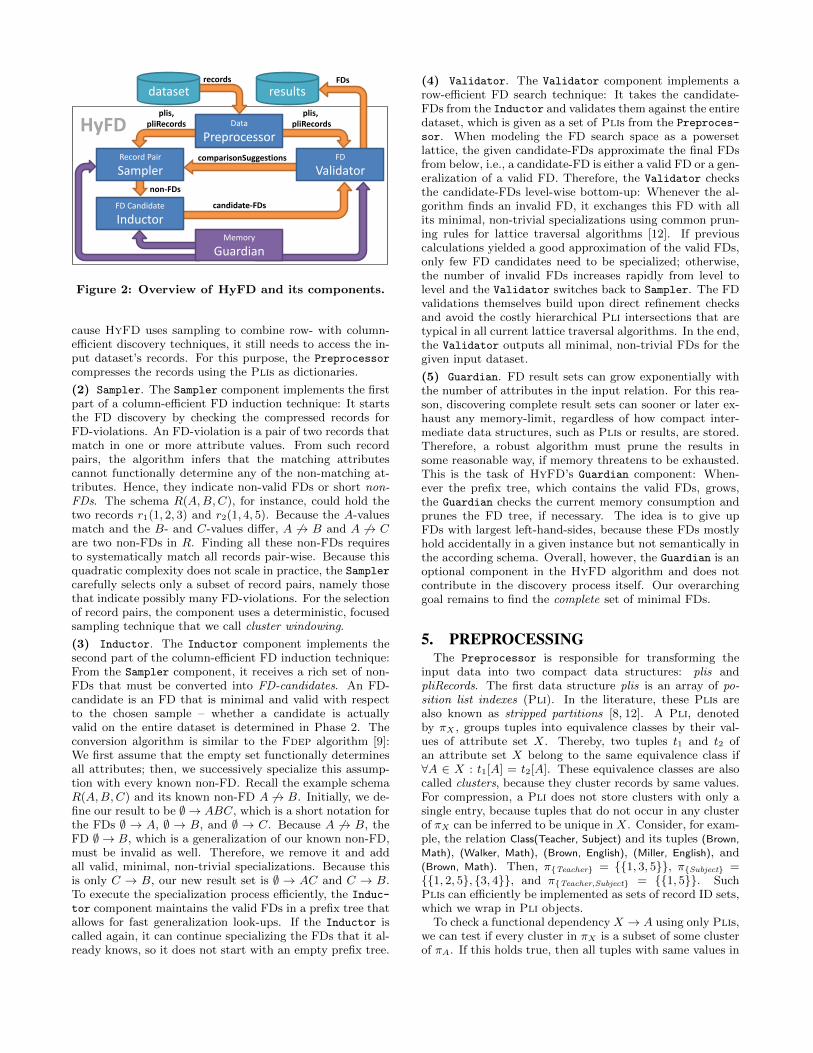
The sampling algorithm. Algorithm 2 implements thefocused sampling strategy introduced above. It requires theplis and pliRecords from the Preprocessor and the compar-isonSuggestions from the Validator. Figure 3 illustratesthe algorithm.

The priority queue efficiencyQueue is a local data struc-ture that ranks the Plis by their sampling efficiency. If theefficiencyQueue is empty (Line 1), this is the first time theSampler is called. In this case, we need to sort all clusters bysome cluster-dependent sorting key (Lines 2 to 4). As shownin Figure 3.1, we sort the records in each cluster of attributeAi’s Pli by their cluster number in attribute Ai−1 and, if

Figure 3: Focused sampling: Sorting of Pli clusters(1); record matching to direct neighbors (2); pro-gressive record matching (3).

numbers are equal or unknown, by the cluster number inAi+1. The intuition here is that attribute Ai−1 has moreclusters than Ai, due to the sorting of plis in the Prepro-

cessor, which makes it a promising key; some unique valuesin Ai−1, on the other hand, do not have a cluster number,so the sorting also checks the Pli of attribute Ai+1 thathas larger clusters than Ai. However, the important pointin choosing sorting keys is not which Ai+/−x to take butto take different sorting keys for each Pli. In this way, theneighborhood of one record differs in each of its Pli clusters.

When the sorting is done, the algorithm initializes theefficiencyQueue with first efficiency measurements. The ef-ficiency of an attribute’s Pli is an object that stores thePli’s sampling performance: It holds the attribute identi-fier, the last window size, the number of comparisons withinthis window, and the number of results, i.e., FD-violationsfirst revealed with these comparisons. An efficiency objectcan calculate its efficiency by dividing the number of resultsby the number of comparisons. For instance, 8 new FD-violations in 100 comparisons yield an efficiency of 0.08. Toinitialize the efficiency object of each attribute, the Sampler

runs a window of size two over the attribute’s Pli clusters(Line 14) using the runWindow ()-function shown in Lines 27to 35. Figure 3.2 illustrates how this function compares alldirect neighbors in the clusters with window size two.

If the Sampler is not called for the first time, the Pli clus-ters are already sorted and the last efficiency measurementsare also present. We must, however, relax the efficiencythreshold (Line 17) and execute the suggested comparisons(Lines 18 and 19). The suggested comparisons are recordspairs that violated at least one FD candidate in Phase 2of the HyFD algorithm so that they probably also violatesome more FDs. With the suggested comparisons, Phase 1incorporates knowledge from Phase 2 to focus the sampling.

No matter whether this is the first or a subsequent callof the Sampler, the algorithm finally starts a progressivesearch for more FD-violations (Lines 20 to 25): It selectsthe efficiency object bestEff with the highest efficiency in theefficiencyQueue (Line 21) and executes the next window sizeon its Pli (Line 25). This updates the efficiency of bestEffso that it might get re-ranked in the priority queue. Figure3.3 illustrates one such progressive selection step for a bestattribute Ai with efficiency 0.08 and next window size three:After matching all records within this window, the efficiencydrops to 0.03, which makes Aj the new best attribute.

The Sampler algorithm continues running ever larger win-dows over the Plis until all efficiencies have fallen below the

current efficiencyThreshold (Line 22). At this point, therow-efficient discovery technique has apparently become in-efficient and the algorithm decides to proceed with a column-efficient discovery technique.

7. INDUCTIONThe Inductor component concludes the column-efficient

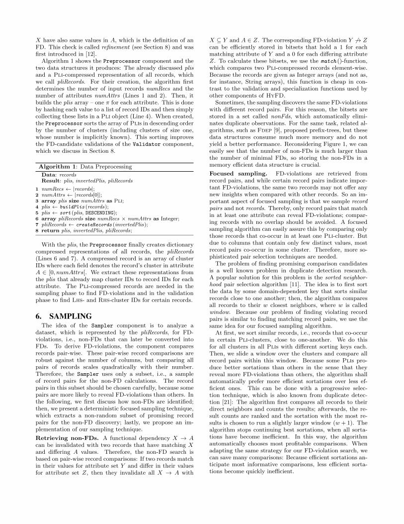
discovery phase and leads over into the row-efficient dis-covery phase. Its task is to convert the nonFds given bythe Sampler component into corresponding minimal FD-candidates fds. These FD-candidates are stored in a datastructure called FDTree, which is a prefix-tree optimized forfunctional dependencies. Figure 4 shows three such FDTreeswith example FDs. First introduced by Flach and Savnikin [9], an FDTree maps the Lhs of FDs to nodes in the treeand the Rhs of these FDs to bitsets, which are attached tothe nodes. A Rhs attribute in the bitsets is marked if it isat the end of an FD’s Lhs path, i.e., if the current path ofnodes describes the entire Lhs to which the Rhs belongs to.

∅ → 𝐴, 𝐵, 𝐶, 𝐷 ∅ → 𝐴, 𝐶, 𝐷 ∅ → 𝐴, 𝐶

(1) Specialize: 𝐷 → 𝐵 (2) Specialize: 𝐴 → 𝐷, 𝐵 → 𝐷, 𝐶 → 𝐷

𝐴 → 𝐵 𝐶 → 𝐵 𝐴, 𝐶 → 𝐷 𝐴, 𝐵 → 𝐷

1 1 1 1

∅ 1 1 1 1

∅

0 1 0 0

𝐶 0 1 0 0

𝐴

1 1 1 1

∅

0 1 0 0

𝐶 0 1 0 1

𝐴

0 0 0 1

𝐶 0 0 0 1

𝐵

𝐴 → 𝐵 𝐶 → 𝐵

(0) Initialize:

Figure 4: Specializing the FDTree with non-FDs.

Algorithm 3 shows the conversion process in detail. TheInductor first sorts the nonFds in descending order by theircardinality, i.e., the number of set bits (Line 1). The sortingof FD-violations is important, because it lets HyFD convertnon-FDs with long Lhss into FD-candidates first and non-FDs with ever shorter Lhss gradually later achieving muchstronger pruning in the beginning. In this way, the prefix-tree of candidate-FDs fds grows much slower, significantlyreducing the costs for early generalization look-ups.

When the Inductor is called for the first time, the FDTreefds has not been created yet and is initialized with a schemaR’s most general FDs ∅ → R, where the attributes in R arerepresented as integers (Line 4); otherwise, the algorithmcontinues with the previously calculated fds. The task is tospecialize the fds with every bitset in nonFds: Each bitsetdescribes the Lhs of several non-FDs (Line 5) and each zero-bit in these bitsets describes a Rhs of a non-FD (Lines 6and 7). Once retrieved from the bitsets, each non-FD isused to specialize the FDTree fds (Line 8).

Figure 4 exemplarily shows the specialization of the initialFDTree for the non-FD D 6→ B in (1): First, the special-

ize -function recursively collects the invalid FD and all itsgeneralizations from the fds (Line 10), because these mustbe invalid as well. In our example, the only invalid FD inthe tree is ∅ → B. HyFD then successively removes thesenon-FDs from the FDTree fds (Line 12). Once removed, thenon-FDs are specialized, which means that the algorithmextends the Lhs of each non-FD to generate still valid spe-cializations (Line 17). In our example, these are A → B

Algorithm 3: Functional Dependency Induction

Data: nonFdsResult: fds

nonFds ← sort (nonFds, CARDINALITY_DESCENDING);1

if fds = null then2

fds ← new FDTree;3

fds.add (∅ → {0, 1, ..., numAttributes});4

for lhs ∈ nonFds do5

rhss ← lhs.clone ().flip ();6

for rhs ∈ rhss do7

specialize (fds, lhs, rhs);8

return fds;9

function specialize (fds, lhs, rhs)invalidLhss ← fds.getFdAndGenerals (lhs, rhs);10

for invalidLhs ∈ invalidLhss do11

fds.remove (invalidLhs, rhs);12

for attr ∈ [0, numAttributes[ do13

if invalidLhs.get(attr) ∨14

rhs = attr then15

continue;16

newLhs ← invalidLhs ∪ attr ;17

if fds.findFdOrGeneral(newLhs, rhs) then18

continue;19

fds.add (newLhs, rhs);20

and C → B. Before adding these specializations, the In-

ductor assures that the new candidate-FD are minimal bysearching the fds for generalizations of the candidate-FDs(Line 18). Figure 4 also shows the result when inducingthree more non-FDs into the FDTree. After specializing thefds with all nonFds, the prefix-tree holds the entire set ofvalid, minimal FDs with respect to these given non-FDs [9].

8. VALIDATIONThe Validator component takes the previously calcu-

lated FDTree fds and validates the contained FD-candidatesagainst the entire input dataset, which is represented by theplis and the invertedPlis. For this validation process, thecomponent uses a row-efficient lattice traversal strategy. Wefirst discuss the lattice traversal; then, we introduce our di-rect candidate validation technique; and finally, we presentthe specialization method of invalid FD-candidates. TheValidator component is shown in detail in Algorithm 4.

Traversal. Usually, lattice traversal algorithms need to tra-verse a huge candidate lattice, because FDs can be every-where (see Figure 1 in Section 3). Due to the previous,sampling-based discovery, HyFD already starts the latticetraversal with a set of promising FD-candidates fds that areorganized in an FDTree. Because this FDTree maps directlyto the FD search space, i.e., the candidate lattice, HyFD canuse it to systematically check all necessary FD candidates:Beginning from the root of the tree, the Validator compo-nent traverses the candidate set breath-first level by level.

When the Validator component is called for the firsttime (Line 1), it initializes the currentLevelNumber to zero(Line 2); otherwise, it continues the traversal from where itstopped before. During the traversal, the set currentLevelholds all FDTree nodes of the current level. So beforeentering the level-wise traversal in Line 5, the Validator

initializes the currentLevel using the getLevel ()-function(Line 3). This function recursively collects all nodes withdepth currentLevelNumber from the prefix-tree fds.

Algorithm 4: Functional Dependency Validation

Data: fds, plis, pliRecordsResult: fds, comparisonSuggestions

if currentLevel = null then1

currentLevelNumber ← 0;2

currentLevel ← fds.getLevel (currentLevelNumber);3

comparisonSuggestions ← ∅;4

while currentLevel 6= ∅ do5

/* Validate all FDs on the current level */invalidFds ← ∅;6

numValidFds ← 0;7

for node ∈ currentLevel do8

lhs ← node.getLhs ();9

rhss ← node.getRhss ();10

validRhss ← refines (lhs, rhss, plis, pliRecords,11

comparisonSuggestions);numValidFds ← numValidFds + |validRhss|;12

invalidRhss ← rhss.andNot (validRhss);13

node.setFds (validRhss);14

for invalidRhs ∈ invalidRhss do15

invalidFds ← invalidFds ∪ (lhs, invalidRhs);16

/* Add all children to the next level */nextLevel ← ∅;17

for node ∈ currentLevel do18

for child ∈ node.getChildren() do19

nextLevel ← nextLevel ∪ child ;20

/* Specialize all invalid FDs */for invalidFd ∈ invalidFds do21

lhs, rhs ← invalidFd ;22

for attr ∈ [0, numAttributes[ do23

if lhs.get(attr) ∨ rhs = attr ∨24

fds.findFdOrGeneral(lhs, attr) ∨25

fds.findFd(attr, rhs) then26

continue;27

newLhs ← lhs ∪ attr ;28

if fds.findFdOrGeneral(newLhs, rhs) then29

continue;30

child ← fds.addAndGetIfNew (newLhs, rhs);31

if child 6= null then32

nextLevel ← nextLevel ∪ child ;33

currentLevel ← nextLevel ;34

currentLevelNumber ← currentLevelNumber + 1;35

/* Judge efficiency of validation process */if |invalidFds| > 0.01 ∗ numV alidFds then36

return fds, comparisonSuggestions;37

return fds, ∅;38

On each level (Line 5), the algorithm first validates all FD-candidates removing those from the FDTree that are invalid(Lines 6 to 16); then, the algorithm collects all child-nodesof the current level to form the next level (Lines 17 to 20); fi-nally, it specializes the invalid FDs of the current level whichgenerates new, minimal FD-candidates for the next level(Lines 21 to 33). The level-wise traversal stops, if the valida-tion process becomes inefficient (Lines 36 and 37). Here, thismeans that more than 1% of the FD-candidates of the cur-rent level were invalid and the search space started growingrapidly. HyFD then returns into the sampling phase. Weuse 1% as a static threshold for efficiency of this phase, butour experiments in Section 10.5 show that any small percent-age performs well here due to the observed high growth rateof invalid FD-candidates. The validation terminates whenthe next level is empty (Line 5) and all FDs in the FDTreefds are valid. This also ends the entire HyFD algorithm.

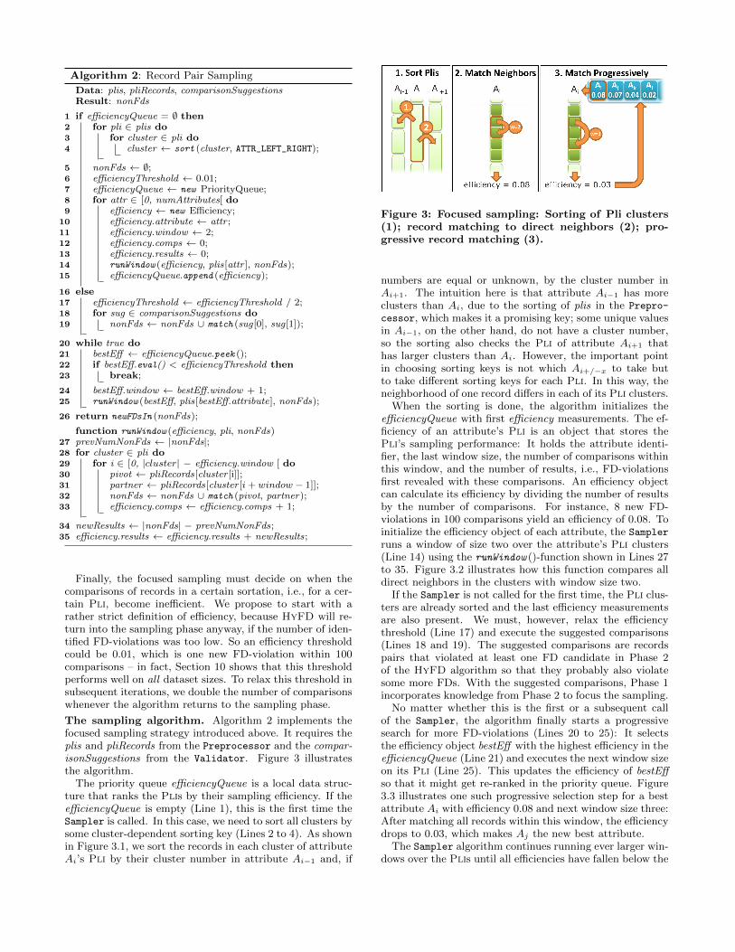
Validation. Each node in an FDTree can harbor multipleFDs with the same Lhs and different Rhss (see Figure 4 inSection 7): The Lhs attributes are described by a node’spath in the tree and the Rhs attributes that form FDs withthe current Lhs are marked. The Validator component val-idates all FD-candidates of a node simultaneously using therefines ()-function (Line 11). This function checks whichRhs attributes are refined by the current Lhs using the plisand pliRecords. The refined Rhs attributes indicate validFDs, while all other Rhs attributes indicate invalid FDs.

Figure 5 illustrates how the refines ()-function works:Let X → Y be the set of FD-candidates that is to be vali-dated. At first, the function selects the pli of the first Lhsattribute X0. Due to the sorting of plis in the Preproces-

sor component, this is the Pli with the most and, hence,the smallest clusters of all Lhs attributes. For each clusterin X0’s Pli, the algorithm iterates all record IDs ri in thiscluster and retrieves the according compressed records fromthe pliRecords. A compressed record contains all cluster IDsin which a record is contained. Hence, the algorithm cancreate one array containing the Lhs cluster IDs of X andone array containing the Rhs cluster IDs of Y . The Lhsarray, then, describes the cluster of ri regarding attributecombination X. To check which Rhs Pli these Lhs clustersrefine, we map the Lhs clusters to the corresponding arrayof Rhs clusters. We fill this map while iterating the recordIDs of a cluster. If an array of Lhs clusters already exists inthis map, the array of Rhs clusters must match the exist-ing one. All non-matching Rhs clusters indicate refinement-violations and, hence, invalid Rhs attributes. The algorithmimmediately stops checking such Rhs attributes so that onlyvalid Rhs attributes survive until the end.

plis[X0]

Validation of 𝑿 → 𝒀

2

5

8

0

4

1

3

6

7

0 2 2

1 1 0

1 1 0

4 0 3

4 0 3

3 3 3

2 1 4

2 1 4

3 0 1

0:

1:

2:

2 4 1

4 5 4

4 5 0

5 2 -

0 2 -

- 4 -

- 0 -

- 0 -

- 3 -

Figure 5: Directly validating FD-candidates X → Y .

In comparison to other Pli-based algorithms, such asTane, HyFD’s validation technique avoids the costly hier-archical Pli intersections. By mapping the Lhs clusters toRhs clusters, the checks are independent of other checks anddo not require intermediate Plis. The direct validation isimportant, because the Validator’s starting FD candidatesare – due to the sampling-based induction part – on muchhigher lattice levels and successively intersecting lower levelPlis would undo this advantage. Furthermore, HyFD canterminate refinement checks very early if all Rhs attributesare invalid, because the results of the intersections, i.e., theintersected Plis are not needed for later intersections. Notstoring intermediate Plis also has the advantage of demand-ing much less memory – most Pli-based algorithms fail atprocessing larger datasets, for exactly this reason [20].

Specialization. The validation of FD candidates identifiesall invalid FDs and collects them in the set invalidFds. Thespecialization part of Algorithm 4, then, extends these in-valid FDs in order to generate new FD candidates for thenext higher level: For each invalid FD represented by lhsand rhs (Line 21), the algorithm checks for all attributesattr (Line 23) if they specialize the invalid FD into a newminimal, non-trivial FD candidate lhs ∪ attr → rhs. Toassure minimality and non-triviality of the new candidate,the algorithm tests the following:

(1) Non-triviality : attr 6∈ lhs and attr 6= rhs (Line 24)

(2) Minimality 1 : lhs 6→ attr (Line 25)

(3) Minimality 2 : lhs ∪ attr 6→ rhs (Lines 24 and 29)

For the minimality checks, the Validator algorithm recur-sively searches for generalizations in the FDTree fds. Thisis possible, because all generalizations in the FDTree havealready been validated and must, therefore, be correct. Thegeneralization look-ups also include the new FD candidateitself, because if this is already present in the tree, it doesnot need to be added again. The minimality checks logicallycorrespond to candidate pruning rules, as used by latticetraversal algorithms, such as Tane, Fun, and Dfd.

If a minimal, non-trivial specialization has been found, thealgorithm adds it to the FDTree fds (Line 31). The addingof a new FD into the FDTree might create a new node inthe graph. To handle these new nodes on the next level,the algorithm must add them to nextLevel. When the spe-cialization has finished with all invalid FDs, the Validator

moves to the next level. If the next level is empty, all FD-candidates have been validated and fds contains all minimal,non-trivial functional dependencies of the input dataset.

9. MEMORY GUARDIANThe memory Guardian is an optional component in HyFD

and enables a best-effort strategy for FD discovery for verylarge inputs. Its task is to observe the memory consumptionand to free resources if HyFD is about to reach the memorylimit. Observing memory consumption is a standard taskin any programming language. So the question is, whatresources the Guardian can free if the memory is exhausted.

The Pli data structures grow linearly with the input data-set’s size and are relatively small. The number of FD-violations found in the sampling step grows exponentiallywith the number of attributes, but it takes quite some at-tributes to exhaust the memory with these compact bit-sets. The data structure that grows by far the fastest isthe FDTree fds, which is constantly specialized by the In-

ductor and Validator components. Hence, this is the datastructure the Guardian must prune.

Obviously, shrinking the fds is only possible by giving upsome results, i.e., giving up completeness of the algorithm.In our implementation of the Guardian, we decided to suc-cessively reduce the maximum Lhs size of our results; weprovide three reasons: First, FDs with a long Lhs usuallyoccur accidentally, meaning that they hold for a particularinstance but not for the relation in general. Second, FDswith long Lhss are less useful in most use cases, e.g., theybecome worse key/foreign-key candidates when used for nor-malization and they are less likely to match a query whenused for query optimization. Third, FDs with long Lhssconsume more memory, because they are physically larger,and preferentially removing them retains more FDs in total.

To restrict the maximum size of the FDs’ Lhss, we need toadd some additional logic into the FDTree: It must hold themaximum Lhs size as a variable, which the Guardian com-ponent can control; whenever this variable is decremented,the FDTree recursively removes all FDs with larger Lhssand sets their memory resources free. The FDTree also re-fuses to add any new FD with a larger Lhs. In this way, theresult pruning works without changing any of the other fourcomponents. However, note that the Guardian componentprunes only such results whose size would otherwise exceedthe memory capacity, which means that the component ingeneral does not take action.

10. EVALUATIONFD discovery has shown to be quadratic in the number of

records n and exponential in the number of attributesm [15].This also holds for HyFD: Phase 1 is in O(mn2 + m22m),because in the worst case n2 records are compared withcomparison costs m and for each of the m possible Rhsattributes, 2m−1 Lhs attribute combinations must be re-fined m − 1 times in the negative cover. Phase 2 is also inO(mn2 + m22m) as shown in [15], because our complexityis the same as for Tane. Note that each phase can (po-tentially) discover all minimal FDs without the other. Thefollowing experiments, however, show that HyFD is able toprocess significantly larger datasets than state-of-the-art FDdiscovery algorithms in less runtime. At first, we introduceour experimental setup. Then, we evaluate the scalability ofHyFD with both a dataset’s number of rows and columns.Afterwards, we show that HyFD performs well on differentdatasets. In all these experiments, we compare HyFD toseven state-of-the-art FD discovery algorithms. We, finally,analyze some characteristics of HyFD in more detail anddiscuss the results of the discovery process.

10.1 Experimental setupMetanome. HyFD and all algorithms from related workhave been implemented for the Metanome data profilingframework (www.metanome.de), which defines standard in-terfaces for different kinds of profiling algorithms. Meta-nome also provided the various implementations of the stateof the art. Common tasks, such as input parsing, result for-matting, and performance measurement are standardized bythe framework and decoupled from the algorithms [19].

Hardware. We run all our experiments on a Dell Pow-erEdge R620 with two Intel Xeon E5-2650 2.00 GHz CPUsand 128 GB RAM. The server runs on CentOS 6.4 and usesOpenJDK 64-Bit Server VM 1.7.0 25 as Java environment.

Null Semantics. Real-world data often contains null

values. So a schema R(A,B) could hold the two recordsr1 = (⊥, 1) and r2 = (⊥, 2). Depending on whether wechoose the semantics null = null or the semantics null 6=null, the functional dependency A → B is false or true

respectively. Hence, the null semantics changes the resultsof the FD discovery. Our algorithm HyFD supports bothsettings, which means that the semantics can be switchedin the Preprocessor (Pli-construction) and in the Sampler

(match ()-function) with a parameter. For the experiments,however, we use null = null, because this is how relatedwork treats null values [20].

Datasets. We evaluate HyFD on various synthetic andreal-world datasets. Table 1 in Section 10.4 and Table 2 in

01002003004005006007008009001000

0,1

1

10

100

1000

10000

1000 4000 16000 64000 256000 1024000

FDs

[#]

Ru

nti

me

[se

c]

Rows (ncvoter)

010002000300040005000600070008000900010000

0,1

1

10

100

1000

10000

1000 8000 64000 512000

FDs

[#]

Ru

nti

me

[se

c]

Rows (uniprot)

0200040006000800010000

0,11

10100

100010000

100000

1000 8000 64000 512000

Fun

ctio

nal

De

pe

nd

en

cie

s

Ru

nti

me

[se

c]

Rows (uniprot)

Tane FUN FD_Mine DFD Dep-Miner

FastFDs Fdep HyFD FDs

Figure 6: Row scalability on ncvoter and uniprot.

Section 10.5 give an overview of these datasets. The datashown in Table 1 was already used in [20]. We also usethe plista [13] dataset containing web log data, the uniprot1

dataset storing protein sequences, and the ncvoter2 datasetlisting public voter statistics. The datasets listed in Table 2have never been analyzed for FDs before, because they aremuch larger than the datasets of Table 1 and most of themcannot be processed with any of the related seven FD dis-covery algorithms within reasonable time (<1 month) andmemory (<100 GB): The CD dataset contains CD-productdata, the synthetic TPC-H dataset models business data,the PDB dataset stores protein sequence data, and theSAP R3 dataset holds data of a real SAP R3 ERP system.

10.2 Varying the number of rowsOur first experiment measures the runtime of HyFD on

different row numbers. The experiment uses the ncvoterdataset with 19 columns and the uniprot dataset with 30columns. The results, which also include the runtimes of theother seven FD discovery algorithms, are shown in Figure 6.A series of measurements stops if either the memory con-sumption exceeded 128 GB or the runtime exceeded 10,000seconds. The dotted line shows the number of FDs in theinput using the second y-axis: This number first increases,because more tuples invalidate more FDs so that more largerFDs arise; then it decreases, because even the larger FDs getinvalidated and no further minimal specializations exist.

With our HyFD algorithm, we could process the 19 col-umn version of the ncvoter dataset in 97 seconds and the30 column version of the uniprot dataset in 89 seconds forthe largest row size. This makes HyFD more than 20 timesfaster on ncvoter and more than 416 times faster on uniprotthan the best state-of-the-art algorithm respectively. Thereason why HyFD performs so much better than currentlattice traversal algorithms is the fact that the number ofFD-candidates that need to be validated against the manyrows is greatly reduced by the Sampler component.

1www.uniprot.org2www.ncsbe.gov/ncsbe/data-statistics

1

10

100

1000

10000

100000

1000000

10000000

0,1

1

10

100

1000

10000

100000

10 20 30 40 50 60

FDs

[#]

Ru

nti

me

[se

c]

Columns (uniprot)

1

10

100

1000

10000

100000

1000000

0,1

1

10

100

1000

10000

10 20 30 40 50 60

FDs

[#]

Ru

nti

me

[se

c]

Columns (plista)

0200040006000800010000

0,11

10100

100010000

100000

1000 8000 64000 512000

Fun

ctio

nal

De

pe

nd

en

cie

s

Ru

nti

me

[se

c]

Rows (uniprot)

Tane FUN FD_Mine DFD Dep-Miner

FastFDs Fdep HyFD FDs

Figure 7: Column scalability on uniprot and plista.

10.3 Varying the number of columnsIn our second experiment, we measure HyFD’s runtime on

different column numbers using the uniprot dataset and theplista dataset with 1,000 records each. Again, we plot themeasurements of HyFD with the measurements of the otherFD discovery algorithms and cut the runtimes at 10,000 sec-onds. Figure 7 shows the result of this experiment.

We first notice that HyFD’s runtime rather scales withthe number of FDs, i.e., with the result size than with thenumber of columns. This is a desirable behavior, becausethe increasing effort is compensated by an also increasinggain. We further see that HyFD again outperforms allexisting algorithms. The improvement factor is, however,smaller in this experiment, because the two datasets are with1,000 rows so small that comparing all pairs of records, asFdep does, is feasible and probably the best way to pro-ceed. HyFD is still slightly faster than Fdep, because itdoes not compare all record pairs; the overhead of creat-ing Plis is compensated by then being able to compare Plicompressed records rather than String-represented records.

10.4 Varying the datasetsTo show that HyFD is not sensitive to any dataset pe-

culiarity, the next experiment evaluates the algorithm onmany different datasets. For this experiment, we set a timelimit (TL) of 4 hours and a memory limit (ML) of 100 GB.Table 1 summarizes the runtimes of the different algorithms.

The measurements show that HyFD was able to processall datasets and that it usually performed best. There areonly two runtimes, namely those for the fd-reduced-30 andfor the uniprot dataset, that are in need of explanation:First, the fd-reduced-30 dataset is a generated dataset thatexclusively contains random values. Due to these randomvalues, all FDs are accidental and do not have any semanticmeaning. Also, all FDs are of same size, i.e., 99% of the89,571 minimal FDs reside on lattice level three and none ofthem above this level. Thus, bottom-up lattice traversal al-gorithms, such as Tane and Fun, and algorithms that havebottom-up characteristics, such as Dep-Miner and Fast-

Dataset Cols Rows Size FDs Tane Fun Fd Mine Dfd Dep-Miner FastFDs Fdep HyFD[#] [#] [KB] [#] [12] [18] [25] [1] [16] [24] [9]

iris 5 150 5 4 1.1 0.1 0.2 0.2 0.2 0.2 0.1 0.1balance-scale 5 625 7 1 1.2 0.1 0.2 0.3 0.3 0.3 0.2 0.1chess 7 28,056 519 1 2.9 1.1 3.8 1.0 174.6 164.2 125.5 0.2abalone 9 4,177 187 137 2.1 0.6 1.8 1.1 3.0 2.9 3.8 0.2nursery 9 12,960 1,024 1 4.1 1.8 7.1 0.9 121.2 118.9 46.8 0.5breast-cancer 11 699 20 46 2.3 0.6 2.2 0.8 1.1 1.1 0.5 0.2bridges 13 108 6 142 2.2 0.6 4.2 0.9 0.5 0.6 0.2 0.1echocardiogram 13 132 6 527 1.6 0.4 69.9 1.2 0.5 0.5 0.2 0.1adult 14 48,842 3,528 78 67.4 111.6 531.5 5.9 6039.2 6033.8 860.2 1.1letter 17 20,000 695 61 260.0 529.0 7204.8 6.0 1090.0 1015.5 291.3 3.4ncvoter 19 1,000 151 758 4.3 4.0 ML 5.1 11.4 1.9 1.1 0.4hepatitis 20 155 8 8,250 12.2 175.9 ML 326.7 5576.5 9.5 0.8 0.6horse 27 368 25 128,727 457.0 TL ML TL TL 385.8 7.2 7.1fd-reduced-30 30 250,000 69,581 89,571 41.1 77.7 ML TL 377.2 382.4 TL 513.0plista 63 1,000 568 178,152 ML ML ML TL TL TL 26.9 21.8flight 109 1,000 575 982,631 ML ML ML TL TL TL 216.5 53.4uniprot 223 1,000 2,439 >2,437,556 ML ML ML TL TL TL ML >5254.7

Results larger than 1,000 FDs are only counted TL: time limit of 4 hours exceeded ML: memory limit of 100 GB exceeded

Table 1: Runtimes in seconds for several real-world datasets (extended from [20])

FDs, perform very well on such an unusual dataset. Theruntime of HyFD, which is about 9 minutes, is an adequateruntime for any dataset with 30 columns and 250,000 rows.

The uniprot dataset is another extreme, but real-worlddataset: Because it comprises 223 columns, the total num-ber of minimal FDs in this dataset is much larger than 100million. This is, as Figure 7 shows, due to the fact thatthe number of FDs in this dataset grows exponentially withthe number of columns. For this reason, we limited HyFD’sresult size to 4 GB and let the algorithm’s Guardian com-ponent assure that the result does not become larger. Inthis way, HyFD discovered all minimal FDs with a Lhs ofup to four attributes; all FDs on lattice level five and abovehave been successively pruned, because they would exceedthe 4 GB memory limit. So HyFD discovered the first 2.5million FDs in about 1.5 hours. One can compute more FDson uniprot with HyFD using more memory, but the entireresult set is – at the time – impossible to store.

The datasets in Table 1 brought all state-of-the-art al-gorithms to their limits, but they are still quite small incomparison to most real-world datasets. Therefore, we alsoevaluated HyFD on much larger datasets. This experimentreports only HyFD’s runtimes, because no other algorithmcan process the datasets within reasonable time and memorylimits. Table 2 lists the results for the single-threaded imple-mentation of HyFD (left column) that we also used in theprevious experiments and a multi-threaded implementation(right column), which we explain below.

The measurements show that HyFD’s runtime dependson the number of FDs, which is fine, because the increasedeffort pays off in more results. Intuitively, the more FDsare to be validated, the longer the discovery takes. But

Dataset Cols Rows Size FDs HyFD[#] [#] [MB] [#] [s/m/h/d]

TPC-H.lineitem 16 6 m 1,051 4 k 39 m 4 mPDB.POLY SEQ 13 17 m 1,256 68 4 m 3 mPDB.ATOM SITE 31 27 m 5,042 10 k 12 h 64 mSAP R3.ZBC00DT 35 3 m 783 211 4 m 2 mSAP R3.ILOA 48 45 m 8,731 16 k 35 h 8 hSAP R3.CE4HI01 65 2 m 649 2 k 17 m 10 mNCVoter.statewide 71 1 m 561 5 m 10 d 31 hCD.cd 107 10 k 5 36 k 5 s 3 s

Table 2: Single- and multi-threaded runtimes onlarger real-world datasets.

the CD dataset shows that the runtime also depends on thenumber of rows, i.e., the FD-candidate validations are muchless expensive if only a few values need to be checked. Ifboth the number of rows and columns becomes large, whichis when they exceed 50 columns and 10 million rows, HyFDmight run multiple days. This is due to the exponentialcomplexity of the FD-discovery problem. However, HyFDwas able to process all such datasets and because no otheralgorithm is able to achieve this, obtaining a complete resultwithin some days is the first actual solution to the problem.

Multiple threads. We introduced and tested a single-threaded implementation of HyFD to compare its runtimewith the single-threaded state-of-the-art algorithms. HyFDcan, however, easily be parallelized, because the compar-isons in the Sampler component are like the validations inthe Validator component independent of one another. Weimplemented these simple parallelizations and the runtimesreduced to the measurements shown in the right columnof Table 2 running 32 parallel threads. Compared to theparallel FD discovery algorithm ParaDe [10], HyFD is 8x(POLY SEQ), 38x (lineitem), 89x (CE4HI01 ), and 1178x(cd) faster due to its novel, hybrid search strategy – for theother datasets, we stopped ParaDe after two weeks.

10.5 In-depth experimentsMemory consumption. Many FD discovery algorithmsdemand a lot of main memory to store intermediate datastructures. The following experiment contrasts the memoryconsumption of HyFD with its three most efficient com-petitors Tane, Dfd, and Fdep on different datasets (thememory consumption of Fun and Fd Mine is worse thanTane’s; Dep-Miner and FastFDs are similar to Fdep [20]).To measure the memory consumption, we limited the avail-able memory successively to 1 MB, 2 MB, ..., 10 MB, 15 MB,..., 100 MB, 110 MB, ..., 300 MB, 350 MB, ..., 1 GB, 2 GB,..., 10 GB, 15 GB, ..., 100 GB and stopped increasing thememory when an algorithm finished without memory issues.Table 3 lists the results. Note that the memory consumptionis given for complete results and HyFD can produce smallerresults on less memory using the Guardian component. Be-cause Dfd takes more than 4 hours, which is our time limit,to process horse, plista, and flight, we could not measure thealgorithm’s memory consumption on these datasets.

Dataset Tane Dfd Fdep HyFDhepatitis 400 MB 300 MB 9 MB 5 MBadult 5 GB 300 MB 100 MB 10 MBletter 30 GB 400 MB 90 MB 25 MBhorse 25 GB - 100 MB 65 MBplista > 100 GB - 800 MB 110 MBflight > 100 GB - 900 MB 200 MB

Table 3: Memory consumption

Due to the excessive construction of Plis, Tane of courseconsumes the most memory. Dfd manages the Plis in aPli-store using a least-recently-used strategy to discard Pliswhen memory is exhausted, but the minimum number of re-quired Plis is still very large. Also, Dfd becomes very slowon low memory. Fdep has a relatively small memory foot-print, because it does not use Plis at all. HyFD uses thesame data structures as Tane and Fdep and some addi-tional data structures, such as the comparison suggestions,but it still has the overall smallest memory consumption: Incontrast to Tane, HyFD generates much fewer candidatesand requires only the single-column Plis for its direct vali-dation technique; in contrast to Fdep, it stores the non-FDsin bitsets rather than index lists and uses the Plis insteadof the original data for the record comparisons.

Efficiency threshold. HyFD requires a parameter thatdetermines when Phase 1 or Phase 2 become inefficient: Itstops the record matching in the Sampler component if lessthan x percent matches delivered new FD-violations and itstops the FD-candidate validations in the Validator com-ponent if more than x percent candidates have shown to beinvalid. In the explanation of the algorithm and in all previ-ous experiments, we set this parameter to 1% regardless ofthe datasets being analyzed. The following experiment eval-uates different parameter settings on the ncvoter statewidedataset with ten thousand records.

0

3

6

9

12

0

50

100

150

200

0,01 0,1 1 10 100

Swit

ches

[#

]

Ru

nti

me

[se

c]

Parameter [%] HyFD Switches

Figure 8: Effect of HyFD’s only parameter on 10thousand records of the ncvoter statewide dataset.

The first line in Figure 8 plots HyFD’s runtime for param-eter values between 0.01% and 100%. It shows that HyFD’sperformance is not very sensitive to the efficiency thresholdparameter. In fact, the performance is almost the same forany value between 0.1% and 10%. This is because the effi-ciency of either phase falls suddenly and fast so that all lowefficiency values are met quickly: The progressive samplingidentifies most matches very early and the validation gener-ates many new, largely also invalid FD-candidates for everycandidate tested as invalid.

However, if we set the parameter higher than 10%, thenHyFD starts validating some lattice levels with too manyinvalid FD-candidates, which affects the performance neg-atively; if we, on the other hand, set the value lower than0.1%, HyFD invests too much time on sampling than ac-

tually needed, which means that it keeps matching recordsalthough all results have already been found. We observedthe same effects an different dataset, so we propose 1% asthe default efficiency threshold for HyFD.

The second line in Table 8 depicts the number of switchesfrom Phase 2 back into Phase 1 that HyFD made with thedifferent parameter settings. We observe that four to fivephase-switches are necessary on ncvoter statewide and do-ing fewer or more switches is disadvantageous for the per-formance. Note that HyFD did these switches on differentlattice-levels depending on the parameter setting, i.e., withlow thresholds it switches earlier; with high thresholds later.

10.6 Result analysisThe number of FDs that HyFD can discover is very large.

In fact, the size of the discovered metadata can easily ex-ceed the size of the original dataset (see the uniprot datasetin Section 10.4). A reasonable question is, hence, whethercomplete results, i.e., all minimal FDs, are actually needed.Schema normalization, for instance, requires only a smallsubset of FDs to transform a current schema into a newschema with smaller memory footprint. Data integrationalso requires only a subset of all FDs, namely those thatoverlap with a second schema. In short, most use-cases forFDs indeed require only a subset of all results.

However, one must inspect all functional dependencies toidentify these subsets: Schema normalization, for instance,is based on closure calculation and data integration is basedon dependency mapping, both requiring complete FD resultsets to find the optimal solutions. Furthermore, in queryoptimization, a subset of FDs that optimizes a given queryworkload by 10% is very good at first sight, but if a differentsubset of FDs could have saved 20% of the query load, onewould have missed some high optimization potential. Forthese reasons and because we cannot know which other usecases HyFD will have to serve, we discover all functionaldependencies – or at least as many as possible.

11. CONCLUSION & FUTURE WORKIn this paper, we proposed HyFD, a hybrid FD discovery

algorithm that discovers all minimal, non-trivial functionaldependencies in relational datasets. Because HyFD com-bines row- and column-efficient discovery techniques, it isable to process datasets that are both long and wide. Thismakes HyFD the first algorithm that can process datasets ofrelevant real-world size, i.e., datasets with more than 50 at-tributes and a million records. On smaller datasets, whichsome other FD discovery algorithms can already process,HyFD offers the smallest memory footprints and the fastestruntimes; in many cases, our algorithm is orders of magni-tude faster than the best state-of-the-art algorithm. Becausethe number of FDs grows exponentially with the number ofattributes, we also proposed a component that dynamicallyprunes the result set, if the available memory is exhausted.

A task for future work is the development of use-case-specific algorithms that leverage FD result sets for schemanormalization, query optimization, data integration, datacleansing, and many other tasks. In addition, knowledge ofthe use-case might help develop specific semantic pruningrules to further speed-up detection. The only reasonablesemantic pruning we found was removing FDs with largestleft-hand-sides, because these are most prone to being acci-dental, and we only apply it when absolutely necessary.

Acknowledgements. We thank Tobias Bleifuß for the ideaof compressing non-FDs as bitsets and the authors of [20]and [10] for providing code and data for our comparativeevaluation.

12. REFERENCES[1] Z. Abedjan, P. Schulze, and F. Naumann. DFD:

Efficient functional dependency discovery. InProceedings of the International Conference onInformation and Knowledge Management (CIKM),pages 949–958, 2014.

[2] R. Agrawal and R. Srikant. Fast algorithms for miningassociation rules in large databases. In Proceedings ofthe International Conference on Very Large Databases(VLDB), pages 487–499, 1994.

[3] P. Bohannon, W. Fan, and F. Geerts. Conditionalfunctional dependencies for data cleaning. InProceedings of the International Conference on DataEngineering (ICDE), pages 746–755, 2007.

[4] C. R. Carlson, A. K. Arora, and M. M. Carlson. Theapplication of functional dependency theory torelational databases. Computer Journal, 25(1):68–73,1982.

[5] E. F. Codd. A relational model of data for largeshared data banks. Communications of the ACM,13(6):377–387, 1970.

[6] E. F. Codd. Further normalization of the data baserelational model. IBM Research Report, San Jose,California, RJ909, 1971.

[7] G. Cormode, L. Golab, K. Flip, A. McGregor,D. Srivastava, and X. Zhang. Estimating theconfidence of conditional functional dependencies. InProceedings of the International Conference onManagement of Data (SIGMOD), pages 469–482,2009.

[8] S. S. Cosmadakis, P. C. Kanellakis, and N. Spyratos.Partition semantics for relations. Journal of Computerand System Sciences, 33(2):203–233, 1986.

[9] P. A. Flach and I. Savnik. Database dependencydiscovery: a machine learning approach. AICommunications, 12(3):139–160, 1999.

[10] E. Garnaud, N. Hanusse, S. Maabout, and N. Novelli.Parallel mining of dependencies. In Proceedings of theInternational Conference on High PerformanceComputing & Simulation (HPCS), pages 491–498,2014.

[11] M. A. Hernandez and S. J. Stolfo. Real-world data isdirty: Data cleansing and the merge/purge problem.Data Mining and Knowledge Discovery, 2(1):9–37,1998.

[12] Y. Huhtala, J. Karkkainen, P. Porkka, andH. Toivonen. TANE: An efficient algorithm fordiscovering functional and approximate dependencies.The Computer Journal, 42(2):100–111, 1999.

[13] B. Kille, F. Hopfgartner, T. Brodt, and T. Heintz.The plista dataset. In Proceedings of the International

Workshop and Challenge on News RecommenderSystems, 2013.

[14] W. Li, Z. Li, Q. Chen, T. Jiang, and H. Liu.Discovering functional dependencies in verticallydistributed big data. Proceedings of the InternationalConference on Web Information Systems Engineering(WISE), pages 199–207, 2015.

[15] J. Liu, J. Li, C. Liu, and Y. Chen. Discoverdependencies from data – a review. IEEETransactions on Knowledge and Data Engineering(TKDE), 24(2):251–264, 2012.

[16] S. Lopes, J.-M. Petit, and L. Lakhal. Efficientdiscovery of functional dependencies and Armstrongrelations. In Proceedings of the InternationalConference on Extending Database Technology(EDBT), pages 350–364, 2000.

[17] R. J. Miller, M. A. Hernandez, L. M. Haas, L.-L. Yan,H. Ho, R. Fagin, and L. Popa. The Clio project:Managing heterogeneity. SIGMOD Record,30(1):78–83, 2001.

[18] N. Novelli and R. Cicchetti. FUN: An efficientalgorithm for mining functional and embeddeddependencies. In Proceedings of the InternationalConference on Database Theory (ICDT), pages189–203, 2001.

[19] T. Papenbrock, T. Bergmann, M. Finke, J. Zwiener,and F. Naumann. Data profiling with metanome.Proceedings of the VLDB Endowment,8(12):1860–1871, 2015.

[20] T. Papenbrock, J. Ehrlich, J. Marten, T. Neubert,J.-P. Rudolph, M. Schonberg, J. Zwiener, andF. Naumann. Functional dependency discovery: Anexperimental evaluation of seven algorithms.Proceedings of the VLDB Endowment,8(10):1082–1093, 2015.

[21] T. Papenbrock, A. Heise, and F. Naumann.Progressive duplicate detection. IEEE Transactions onKnowledge and Data Engineering (TKDE),27(5):1316–1329, 2015.

[22] G. N. Paulley. Exploiting functional dependence inquery optimization. Technical report, University ofWaterloo, 2000.

[23] J. D. Ullman. Principles of Database andKnowledge-Base Systems: Volume II: The NewTechnologies. W. H. Freeman & Co., New York, NY,USA, 1990.

[24] C. Wyss, C. Giannella, and E. Robertson. FastFDs: Aheuristic-driven, depth-first algorithm for miningfunctional dependencies from relation instancesextended abstract. In Proceedings of the InternationalConference of Data Warehousing and KnowledgeDiscovery (DaWaK), pages 101–110, 2001.

[25] H. Yao, H. J. Hamilton, and C. J. Butz. FD Mine:discovering functional dependencies in a databaseusing equivalences. In Proceedings of the InternationalConference on Data Mining (ICDM), pages 729–732,2002.