a hybrid discrete firefly algorithm for solving multi ... · pdf fileannealing (sa), variable...

Loughborough UniversityInstitutional Repository

A hybrid discrete fireflyalgorithm for solving

multi-objective flexible jobshop scheduling problems

This item was submitted to Loughborough University's Institutional Repositoryby the/an author.

Citation: KARTHIKEYAN, S. ... et al, 2015. A hybrid discrete firefly algo-rithm for solving multi-objective flexible job shop scheduling problems. Inter-national Journal of Bio-Inspired Computation, 7 (6), pp. 386-407.

Additional Information:

• This paper was accepted for publication in the journal International Jour-nal of Bio-Inspired Computation and the definitive published version isavailable at http://dx.doi.org/10.1504/IJBIC.2015.073165

Metadata Record: https://dspace.lboro.ac.uk/2134/17676

Version: Accepted for publication

Publisher: c© Inderscience

Rights: This work is made available according to the conditions of the Cre-ative Commons Attribution-NonCommercial-NoDerivatives 4.0 International(CC BY-NC-ND 4.0) licence. Full details of this licence are available at:https://creativecommons.org/licenses/by-nc-nd/4.0/

Please cite the published version.

https://dspace.lboro.ac.uk/2134/17676

1

S. Karthikeyan* and P. Asokan Department of Production Engineering, National Institute of Technology,

Tiruchirappalli – 620015, Tamilnadu, India

E-mail: [email protected]

[email protected]

* Corresponding author

S. Nickolas Department of Computer Applications,

National Institute of Technology,

Tiruchirappalli – 620015, Tamilnadu, India


Tom Page Loughborough Design School, LDS.1.18

Loughborough University,

Leicestershire, LE11 3TU, UK


Biographical Notes: S. Karthikeyan received his graduation in Mechanical Engineering from

University of Madras, Chennai, India and post-graduation in Manufacturing Technology from

National Institute of Technology, Tiruchirappalli, India. Currently, he is pursuing PhD in the Department of Production Engineering, National Institute of Technology, Tiruchirappalli, India.

His research interests focus on scheduling and manufacturing system optimization. He is an active

life member of Indian Society of Technical Education.

P. Asokan received his graduation in Mechanical Engineering and post-graduation in

Manufacturing Technology from Regional Engineering College, Tiruchirappalli, India. He received

his PhD from Bharathidasan University, Tiruchirappalli, India in 1998. Presently he is serving as a Professor in Department of Production Engineering, National Institute of Technology,

Tiruchirappalli, India. He has nearly 24 years of teaching experience. His area of specialization is

operation management and optimization in manufacturing. He has published 55 papers in international journals and 33 papers in international conferences.

S. Nickolas is currently working as Associate Professor in the Department of Computer Applications, National Institute of Technology, Tiruchirappalli, India. He received his M.E. in the

field of Computer Science from Regional Engineering College, Tiruchirappalli, India and PhD

from National Institute of Technology, Tiruchirappalli, India in 2007. He has published 20 papers

in International Conferences and 10 papers in International Journals. His area of interest includes Database systems, Data mining, Software metrics and Distributed systems.

Tom Page is a Senior Lecturer of Electronic Product Design at Loughborough University. He received his PhD from the University of Hertfordshire. His research interests are in engineering

design, value management, technology education and electronic product design. He has been a

consultant for many Small and Medium sized Enterprises in engineering design and electronic product design. His work has been widely published in the form of journal papers, book

contributions, refereed proceedings, refereed conference papers and technical papers.

mailto:[email protected]




2

A hybrid discrete firefly algorithm for solving multi-objective flexible job shop scheduling problems

Abstract

Firefly Algorithm (FA) is a nature-inspired optimization algorithm that can be successfully

applied to continuous optimization problems. However, lot of practical problems are

formulated as discrete optimization problems. In this paper a hybrid discrete firefly

algorithm (HDFA) is proposed to solve the multi-objective flexible job shop scheduling

problem (FJSP). FJSP is an extension of the classical job shop scheduling problem that

allows an operation to be processed by any machine from a given set along different

routes. Three minimization objectives - the maximum completion time, the workload of

the critical machine and the total workload of all machines are considered simultaneously.

This paper also proposes firefly algorithm’s discretization which consists of constructing a

suitable conversion of the continuous functions as attractiveness, distance and movement,

into new discrete functions. In the proposed algorithm discrete firefly algorithm (DFA) is

combined with local search (LS) method to enhance the searching accuracy and

information sharing among fireflies. The experimental results on the well-known

benchmark instances and comparison with other recently published algorithms shows that

the proposed algorithm is feasible and an effective approach for the multi-objective flexible job shop scheduling problems.

Keywords: firefly algorithm; hybrid discrete firefly algorithm; HDFA; flexible job shop

scheduling; FJSP; discrete firefly algorithm; DFA; multi-objective optimization

1. Introduction

Scheduling is the decision-making process which involves the allocation of resources over

a period of time to perform a collection of tasks. Job-shop scheduling problem (JSP) is one

of the hardest combinatorial optimization problems (Jain and Meeran, 1999), in the branch

of production scheduling. The classical JSP consists of scheduling a set of jobs on a set of

machines with the objective to minimize a certain criterion, subject to the constraint that

each job has a specified processing order throughout. It is well known that this problem is

NP-hard (Garey et al., 1976).

The flexible job shop scheduling problem (FJSP) is the generalization of the

classical job shop problem, where operations are allowed to be processed on any machine

from a given set along different routes. Flexible job shop scheduling problem possess

many applications in competitive environment. For example, it is used in flexible

manufacturing systems. A flexible manufacturing system consists of several computer

numerical control (CNC) machines. A CNC machine is a multitasking machine. So

flexible job shop scheduling is applicable for flexible manufacturing systems. Bruker and

Schlie (1990) were among the first to address this problem. It is closer to the real

manufacturing situation. It incorporates all difficulties and complexities of its predecessor

JSP and is more complex than JSP due to the need to determine the assignment of

operations to machines.

Due to the complexity of FJSP, no exact method has so far been introduced to

tackle these problems within a reasonable amount of time. Hence, a variety of heuristic

procedures such as dispatching rules, local search and meta-heuristic algorithms such as

tabu search (TS), genetic algorithm (GA), particle swarm optimization (PSO), simulated

3

annealing (SA), variable neighbourhood search (VNS), artificial bee colony algorithm

(ABC), artificial immune algorithm (AIA) and biogeography-based optimization algorithm

(BBO) have been applied to solve these problems and find the optimal or near optimal

schedule in a reasonable time. FJSP could be decomposed into two sub-problems of

routing and scheduling. The routing sub-problem assigns each operation to a machine out

of a set of capable machines authorized for each job. The scheduling sub-problem involves

sequencing the operations assigned to the machines in order to obtain a feasible schedule

that minimizes a predefined objective (Xia and Wu, 2005).

For solving the realistic case with more than two jobs, two types of approach have

been used: hierarchical approach and integrated approach. Hierarchical approach was

firstly proposed by Brandimarte (1993). In hierarchical approach, assigning operations to

machines and the sequencing of operations on the machines are accomplished separately.

Its basic idea is to divide a hard problem into two simpler sub-problems in order to

decrease the complexity. Kacem et al. (2002a) proposed a localization approach to solve

the resource assignment problem, and an evolutionary approach controlled by the

assignment model for FJSP. Xia and Wu (2005) used particle swarm optimization (PSO) to

assign operations to machines and simulated annealing (SA) algorithm to schedule

operation on each machine for solving multi-objective FJSP. However, the integrated

approach solves the assignment sub-problem and sequencing sub-problem simultaneously,

such as greedy heuristics (Mati et al., 2001), simulated annealing (SA) algorithm (Hapke et

al., 2000), genetic algorithm (Chan et al., 2006), tabu search (Scrich et al., 2004) and

particle swarm optimization (PSO) algorithm (Girish and Jawahar, 2009).

Most of the research on FJSP has been concentrated on mono-objective. However

several objectives must be considered simultaneously in the real world production situation

and these objectives often conflict with each other. In the recent years, multi-objective

FJSP (MOFJSP) has gained attention of some researchers. The methods to solve the

MOFJSP can be roughly classified into two types: weighted summation approach and

Pareto-based approach. The weighted summation approach solves the MOFJSP by

transforming it to a mono-objective one by giving each objective a weight. The Pareto-

based approach solves the MFJSP based on the Pareto optimality concept and aims at

generating the set of Pareto optimal solutions. The existing algorithms belonging to the

first type include localization approach to solve the resource assignment problem (Kacem

et al., 2002a), hybrid optimization approach with PSO and SA (Xia & Wu, 2005), hybrid

genetic algorithm (GA) (Gao et al., 2008), hybrid PSO algorithm with tabu search (TS)

(Zhang et al., 2009),) efficient search method (Xing et al., 2009), effective hybrid tabu

search algorithm (HTSA) (Li et al., 2010), hybrid PSO algorithm and data mining

(Karthikeyan et al., 2012). The existing algorithms belonging to the second type include

the Pareto based algorithm which combines fuzzy logic and evolutionary algorithms

(Kacem et al., 2002b), multi-objective genetic algorithm (MOGA) (Wang et al., 2010),

Memetic Algorithm based on NSGAII (Frutos et al., 2010), Pareto- based discrete artificial

bee colony algorithm (Li et al., 2011), multi objective particle swarm optimization

(Moslehi and Mahnam, 2011), multi objective evolutionary algorithm (Chiang and Lin,

2013), and hybrid shuffled frog-leaping algorithm (HSFLA) (Li et al., 2012).

Evolutionary Algorithms are stochastic search method that mimics the metaphor of

natural biological evolution and/or the social behaviour of species. García-Gonzalo et al.

(2012) presented a brief historical review of PSO, insisting in the importance of the

stochastic stability analysis of the particle trajectories in order to achieve convergence. Bat

algorithm (BA) is a bio-inspired algorithm developed by Yang, (2010) based on the

echolocation features of microbats. Recently Yang and He (2013) provided a review of the

bat algorithm and its new variants. Artificial plant optimization algorithm is a recent

4

proposed population based stochastic algorithm. It is inspired by the natural plant growing

process. Bing Yu et al. (2013) used artificial plant optimization algorithm with correlation

branches to test the performance of the unconstrained multi-modal benchmark problems.

Firefly Algorithm (FA) was introduced by Yang, (2008). It is a meta-heuristic algorithm

inspired by the social behaviour of fireflies. Yang (2009) proposed a firefly algorithm for

multimodal optimization applications. Lukasik and Zak (2009) presented a further study on

the firefly algorithm for constrained continuous optimization problems. Sayadi et al.

(2010) presented a discrete firefly algorithm to minimize makespan for the flow shop

scheduling problems. A discrete firefly algorithm was proposed by Jati, (2011) to solve the

travelling salesman problem. Khadwilard et al. (2012) solved the job shop scheduling

problems using firefly algorithm. They also investigated different parameters for the

proposed algorithm and compared the performance with different parameters.

Marichelvam et al. (2012) proposed a discrete firefly algorithm using the SPV rule for the

multi-objective hybrid flow shop scheduling problems. The traditional firefly algorithm is

a population based technique for solving continuous optimization problems, especially for

continuous NP-hard problems. The learning process is based on the real number such that,

the standard firefly algorithm cannot be directly applied to solve the discrete optimization

problems.

To the best of our knowledge, there is no published work dealing with the multi-

objective FJSP by using DFA. Thus, in this paper we proposed a hybrid algorithm

combining DFA with a local search approach to solve the multi-objective FJSP. In the

proposed algorithm, rules are presented for generating the initial population with a high

level of quality. This paper describes firefly algorithm’s discretization, which consists of

constructing a suitable conversion of the continuous functions such as attractiveness,

distance and movement, into new discrete functions. DFA allows an extensive search for

the solution space while the local search method is employed to reassign the machines to

operations and to reschedule the results obtained from DFA, which will enhance the

convergence speed. The objectives considered in this paper are to minimize maximal

completion time, the workload of the critical machine and the total workload of machines

simultaneously.

The remainder of this paper is organized as follows. The formulation and notation

of multi-objective FJSP are introduced in Section 2. Section 3 describes the traditional

firefly algorithm. In Section 4, the proposed approach is presented to solve the FJSP.

Section 5 shows the computational results and its comparison with other algorithms.

Finally, Section 6 provides conclusions and further research.

2. Problem Formulation

The flexible job-shop scheduling problem can be formulated as follows. There is a set of n

jobs J (J = {J1, J2 ...Jn}) supposed to be processed on a set of m machines M (M = {M1,

M2......,Mm}). For each job Ji, consists of a sequence of ni operations. Each operation Oij (i

= 1,2,...,n; j = 1,2,...,ni) of job (Ji) can be processed on any subset Mi,j M of compatible

machines. For job Ji, Pijk denotes the processing time of operation j (Oij) on machine k. The

FJSP is needed to determine both an assignment and sequence of the operations of the

machines in order to satisfy the given criteria. However, the FJSP is more complex and

challenging than the classical JSP because it requires a proper selection of machines from a

set of available machines to process each operation of each job (Ho et al., 2007). The

flexibility of problems can be categorised into partial flexibility and total flexibility. If

there is Mij M for at least one operation, it is partial flexibility FJSP (P-FJSP); while

there is Mi,j = M for each operation, it is total flexibility FJSP (T-FJSP) (Kacem et al.

5

2002a, 2002b).

In this study, the following objectives are to be minimized:

(1) Makespan (Cm) of the jobs, i.e. the completion time of all jobs

(2) Maximal machine workload (Wm), i.e. the maximum working time spent on any

machine

(3) Total workload of the machines (Wt) which represents the total working time over

all machines.

The following assumptions are also considered:

(1) Move time between operations and setup time of machines are ignored.

(2) Machines are independent from each other.

(3) Jobs are independent from each other.

(4) Pre-emption is not allowed, i.e., each operation cannot be interrupted before its

completion on the assigned machine.

(5) At a given time, a machine can execute only one operation.

(6) There are no precedent constraints among the operations of different jobs.

The notations used in this study are listed as follows:

i,h: index of jobs, i, h = 1, 2, . . . , n

j,g: index of operation sequence, j, g = 1, 2, . . . , ni

k: index of machines, k = 1, 2, . . . , m

n: total number of jobs

m: total number of machines

ni: total number of operations of job i

Oij: the jth operation of job i

Mij: the set of available machines for the operation Oij

Pijk: processing time of operation Oij on machine k

tijk: start time of operation Oij on machine k

Cij: completion time of the operation Oij

Ck is the completion time of Mk

Wk is the workload of Mk.

Decision variable

xijk = 1, if machine k is selected for the operation 𝑂𝑖𝑗

0, otherwise

Our model is presented as follows:

min𝑓1 = max1≤𝑘≤𝑚

𝐶𝑘 (1)

min𝑓2 = max1≤k≤m

Wk (2)

min 𝑓3 = 𝑊𝑘

𝑚

𝑘=1

(3)

Subject to:

6

𝐶𝑖𝑗 − 𝐶𝑖(𝑗−1) ≥ 𝑃𝑖𝑗𝑘 𝑋𝑖𝑗𝑘 , 𝑗 = 2,……𝑛𝑖; ∀𝑖, 𝑗 (4)

𝐶𝑕𝑔 − 𝐶𝑖𝑗 − 𝑡𝑕𝑗𝑘 𝑋𝑕𝑔𝑘𝑋𝑖𝑗𝑘 ≥ 0 ∨ 𝐶𝑖𝑗 − 𝐶𝑕𝑔 − 𝑡𝑖𝑗𝑘 𝑋𝑕𝑗𝑖𝑋𝑖𝑗𝑘 ≥ 0 ,

∀ 𝑖, 𝑗 , 𝑕,𝑔 ,𝑘 (5)

𝑋𝑖𝑗𝑘𝑘∈𝑀𝑖𝑗= 1,∀𝑖, 𝑗 (6)

Equation (1) ensures the minimization of maximal completion time of the machines.

Equation (2) ensures the minimization of maximal machine critical workload among all the

machines available. Equation (3) ensures the minimization of total work load of machines.

Inequality (4) ensures the operation precedent constraint. Inequality (5) ensures that each

machine could process only one operation at each time when the first or second condition

mentioned in the constraint satisfies all stated elements. Equation (6) states that one

machine could be selected from the set of machines for each operation.

Many approaches have been formulated to solve the multi-objective optimization. These

approaches can be classified into three categories (Hsu et al., 2002).

(1) Transform the multi-objective problem to a mono-objective problem by a weighted

sum approach

(2) The non-Pareto approach deals with different objectives in a separated way

(3) The Pareto approach based on the Pareto optimality concept.

The objective function in this paper is based on the first type of approach described above.

The weighted sum of the three objective values is taken as the objective function:

Minimize F(c) = W1 × f1 + W2 × f2 + W3 × f3 (7)

Subject to:

W1 + W2 + W3 = 1, 0 ≤ W1, W2, W3 ≤ 1 (8)

where F(c) denotes the combined objective function value of a schedule, f1, f2 and f3 which

denotes the makespan (Cm), maximal machine workload (Wm) and total workload of

machines (Wt) respectively. W1, W2, and W3 represent the weight coefficient for the three

objective values, which could be set for different values depending upon the requirement.

If the decision maker pays more attention to a certain objective, a large weight is defined to

it. Otherwise, a small weight for the given objective can be defined. In this work the

weight coefficients W1, W2, and W3 for the five Kacem instances are set to 0.5, 0.3 and 0.2

according to Xing et al. (2009a, 2009b). The advantage of utilizing the weighted

summation approach is its algorithmic actualization which is effortless and the users can

change the weight of different objectives for satisfying the requirements of decision

makers.

3. Firefly algorithm

Firefly Algorithm (FA) is a recently developed nature-inspired meta-heuristic algorithm.

The firefly algorithm is inspired by the social behaviour of fireflies. Most of the fireflies

produce short and rhythmic flashes and have different flashing behaviour. Fireflies use

these flashes for communication and attracting the potential prey. The swarm of fireflies

7

will move to brighter and more attractive locations by the flashing light intensity that is

associated with the objective function of problems considered, in order to obtain efficient

optimal solutions.

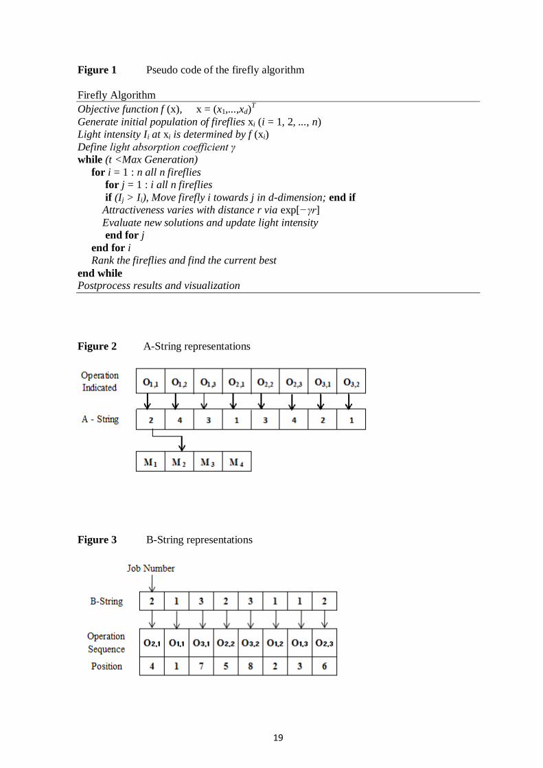
## Insert Figure 1 ##

In essence, FA uses the following three idealized rules (Yang, 2008): (1) all fireflies are

unisex so that one firefly will be attracted to other fireflies regardless of their sex; (2)

attractiveness of a firefly is proportional to their brightness, thus for any two flashing

fireflies, the less brighter one will move towards the brighter one. The attractiveness is

proportional to the brightness and they both increase as their distance decreases. If there is

no brighter one than a particular firefly, it will move randomly; (3) the brightness of a

firefly is determined by the value of the objective function. For a maximization problem,

the brightness may be proportional to the objective function value. For minimization

problem the brightness may be the reciprocal of the objective function value. The basic

steps of the FA are summarized by the pseudo code shown in Figure 1 which consists of

three rules discussed above.

Based on Yang (2009), FA is very efficient in finding the global optimal value with high

success rates. Simulations and results indicate that FA is superior to both PSO and GA in

terms of both efficiency and success rate. These facts give inspiration to investigate how to

find optimal solution using FA in solving FJSP. The challenges are how to compute

discrete distance between two fireflies and how they move in coordination. The following

issues are important in this algorithm.

3.1 Attractiveness

The attractiveness of a firefly is determined by its light intensity. Each firefly has its

distinctive attractiveness β which implies how strong it attracts other members of the

swarm. The form of attractiveness function of a firefly is the following monotonically

decreasing function (Lukasik and Zak, 2009)

𝛽 𝑟 = 𝛽0𝑒−𝛾𝑟𝑚

, 𝑚 ≥ 1 (9)

where r is the distance between two fireflies, β0 is the attractiveness at r = 0 and γ is a fixed

light absorption coefficient.

3.2 Distance

The distance between any two fireflies i and j, at positions xi and xj, respectively can be

defined as a Cartesian distance:

𝑟𝑖𝑗 = 𝑥𝑖 − 𝑥𝑗 = 𝑥𝑖,𝑘 − 𝑥𝑗 ,𝑘 2𝑑

𝑘=1 (10)

where xi,k is the kth

component of the spatial coordinate xi of the ith firefly and d is the

number of dimensions.

3.3 Movement

The movement of a firefly i which is attracted by a more attractive (i.e., brighter) firefly j

is given by the following equation (Lukasik and Zak, 2009)

𝑥𝑖 = 𝑥𝑖 + 𝛽0𝑒−𝛾𝑟𝑖𝑗

2 𝑥𝑗 − 𝑥𝑖 + 𝛼 𝑟𝑎𝑛𝑑 − 1 2 (11)

where the first term is the current position of a firefly, the second term is used for

considering a firefly’s attractiveness to light intensity seen by adjacent fireflies, and the

third term is used for the random movement of a firefly if there is no brighter ones. The

coefficient α is a randomization parameter determined by the problem of interest, while

8

rand is a random number generator uniformly distributed in the space [0, 1]. In this

implementation of the algorithm, we will use β0 = 1.0, α ∈ [0, 1] and the attractiveness or

absorption coefficient γ is in the interval [0.01, 0.15], which guarantees a quick

convergence of the algorithm to the optimal solution.

4. Discrete Firefly Algorithm

The firefly algorithm has been originally developed for solving continuous optimization

problems. The firefly algorithm cannot be applied directly to solve the discrete

optimization problems. In this study, we propose a possible way that can be modified to

solve the class of discrete problems, where the solutions are based on discrete job

permutations. In DFA, the target individual is represented by two vectors: one is for the

machine assignment and the other is for permutation of jobs. Hamming distance is used to

measure the distance between two permutations. The Hamming distance has been already

applied by the researchers in the scheduling problems. Movement is implemented by

breaking the attraction step into two sub steps as β-step and α-step.

## Insert Table 1 ##

4.1 Discrete firefly algorithm for multi-objective FJSP

4.1.1 Solution representation

The FJSP problem is a combination of machine assignment and operation scheduling

decisions, so the solution can be expressed by the assignment of operations on machines

and the processing sequence of operations on the machines. In this study, we used

improved A-string (machine assignment) and B-string (operation scheduling)

representation for each firefly that could be used to solve the multi-objective FJSP

efficiently and avoid the use of a repair mechanism (Zhang et al., 2009).

Machine assignment: An array of integer values is used to represent A-string. The length

of the array is equal to the sum of all operations of all jobs. Each integer value equals the

index of the array of alternative machine set of each operation. An example of A-string

from the problem stated in Table 1 is shown in Figure 2. The length of the A-string is 8.

The value in each cell of the array represents that the particular operation is assigned to

that machine number i.e., 2 is mentioned in the first cell of the array which means that the

operation O1,1 is assigned to the 2nd

machine M2.


Operation Scheduling: B-string has the same length as the A-string as shown in Figure 3.

It consists of a sequence of job numbers in which the job number i occurs ni times. It can

avoid creating an infeasible schedule when replacing each operation by the corresponding

job index. From Table 1, a possible B-string may be 2-1-3-2-3-1-1-2. Read the data from

left to right, the B-string could be translated into a list of ordered operations: O2,1-O1,1-O3,1-

O2,2-O3,2-O1,2-O1,3-O2,3. The operation sequence of B-String may be represented in terms of

position like 4-1-7-5-8-2-3-6. When a particle is decoded, B-string is converted to a

sequence of operations at first. Then each operation is assigned to a processing machine

according to A-string as follows: [(O2,1, M1),(O1,1, M2),(O3,1, M2),(O2,2, M3),(O3,2, M1),(O1,2,

M4),(O1,3, M3),(O2,3, M4)].


4.1.2 Population Initialization

The quality of the initial population has a greater effect on the performance of an

algorithm. A good initial population locates promising areas in the search space and

9

provides enough diversity to avoid premature convergence.

Machine assignment component initial rules: Initiate the machine assignment component

of the population using the following two rules: the operation minimum processing time

rule (Pezzella et al., 2008) denoted by R1, the global machine workload balance rule (Li et

al., 2012) denoted by R2.

Scheduling component initial rules: The scheduling component considers how to sequence

the operations at each machine, i.e., to determine the start time of each operation.

Following are initial approaches for scheduling component: the most work remaining

(MWR) rule (Brandimarte, 1993) denoted by S1, the most number of operations remaining

(MOR) rule (Pezzella et al., 2008) denoted by S2.

Finally, one part of the initial population is achieved by using the above initial approaches

and the remaining population is generated by a simple random rule. To consider both the

problem features and solution quality, in the first part of the population, machine

assignment components and scheduling components are generated according to percentage

of population size given for rules R1, R2, S1, and S2 respectively. All other solutions in the

initial population are generated randomly to enhance the diversity of the population.

4.1.3 Firefly evaluation

Each firefly is represented by A-string and B-string. By using the permutation, each firefly

is evaluated to determine the objective function. The objective function value of each

firefly is associated with the light intensity of the corresponding firefly. In this work, the

evaluation of the goodness of schedule is measured by the combined objective function

which can be calculated using equation (7). Table 2 shows the firefly representation with

combined objective function value for the example problem given in Table 1. The number

of fireflies (population size) used in this problem is 10. The best firefly (Pbest) based on the

combined objective function value is population P-7.


4.1.4 Solution updation

In firefly algorithm, firefly movement is based on light intensity and comparing it between

two fireflies. The attractiveness of a firefly is determined by its brightness which in turn is

associated with the encoded objective function. Thus for any two fireflies, the less bright

one will move towards the brighter one. If no one is brighter than a particular firefly, it will

move randomly. In this work, discretization is done for the following issues:

Distance: There are two possible ways to measure the distance between two permutations:

(a) Hamming distance and (b) the number of the required swaps of the first solution in

order to get the second one. In A-string the distance between any two fireflies i and j, at

positions xi and xj, respectively can be measured by using Hamming distance. The

Hamming distance between two permutations is the number of non-corresponding

elements in the sequence (Kuo et al., 2009). The example of Hamming distance is given as

follows: If there are two A-strings in the FJSP solution space which are P = {2 4 3 1 3 4 2

1} and Pbest = {1 4 1 3 2 2 3 4}, we compare every bit of two strings and record the number

of bits whose machine indices are not equal. Hence, the Hamming distance (P, Pbest) is 7.

The distance between two permutations in the B - string can be measured by using swap

distance. The swap distance is the number of minimal required swaps of one permutation

in order to obtain the other one. For example let us consider B-string representation of two

fireflies P = {4 1 7 5 8 2 3 6} and Pbest = {1 4 7 5 2 3 6 8}. Swap distance (P, Pbest) is

thereby, 4.


10

Attraction and Movement: Attraction and movement has to be implemented and interpreted

for FJSP in the same way as it is intended for the continuous firefly algorithm. In this

study, we can break up an attraction step given in equation (11) into two sub-steps: β-step

and α-step as given in equation (12) and equation (13) respectively. We can do this, since

we know that the result will not change.

𝑥𝑖 = 𝛽 𝑟 𝑥𝑗 − 𝑥𝑖 (12)

𝑥𝑖 = 𝑥𝑖 + 𝛼 𝑟𝑎𝑛𝑑 − 1 2 (13)

The attraction steps α and β are not interchangeable. The β-step must be computed before

the α-step while finding the new position of the firefly.

β – Step: It brings the iterated firefly always closer to another firefly. In other words, after

applying a β-step on a firefly towards the other firefly, their distance is always decreased,

and the decrement is proportional to their former distance. The steps involved in β-step are

as follows:

d = the difference between the elements of best firefly and other firefly

r = hamming distance for A-string and swap distance for B-string

An insertion mechanism and a pair-wise exchange mechanism are used to advance the A-

string and B-string part of each firefly position towards the best firefly position. At first,

the difference between the current position of the firefly and its best position is found by

comparing their corresponding elements of the A-string part and B-string part separately.

All necessary insertions in the A-string part and all necessary pair-wise exchanges in the

B-string part, to make the elements of the current firefly equal to best firefly, are found and

stored in d. Counting the number of insertions and pair-wise exchanges between two

firefly will give the hamming distance and swap distance respectively, which is stored in r.

Then we need to compute the β probability. Since it is often faster to calculate 1 / (1 + r2)

than an exponential function (Pal et al., 2012), the equation (9) can be approximated as

𝛽 𝑟 = 𝛽0 1 + 𝛾𝑟2 (14)

Secondly, each insertion/pair-wise exchange in the set d is accessed and a random number

rand ( ) is generated in the range (0, 1). If rand ( ) ≤ β, then the corresponding

insertion/pair-wise exchange is performed on the elements of the current firefly. This

procedure moves the current firefly to the global best position, which is controlled by the β

probability. This procedure is repeated for all the fireflies.

α – Step: It is much simpler than the β-step. In equation (13) the random movement of

firefly α (rand – 1/2) is approximated as α (randint) given in equation (15) which allows us

to shift the permutation into one of the neighbouring permutations. α - step is applied by

𝑥𝑖 = 𝑥𝑖 + 𝛼(𝑟𝑎𝑛𝑑𝑖𝑛𝑡 ) (15)

choosing an element position using α (randint) and swap with another position in the string

which is also chosen at random. The random number randint is a positive integer generated

between the minimum and maximum number of elements in the string.

Table 3 illustrates the firefly position update procedure for population 1 in the first

generation. The parameters used in this illustration are as follows: β0 = 1, γ = 0.1, α = 1.

The improvement of objective function value F(c) from 19.9 to 14.8 shows the movement

of firefly from its current solution to the best firefly solution. The objective function of

each firefly population obtained in the first generation replaces its previous value (P), if its

current solution is better than the previously stored firefly solution. The best solution of the

first iteration replaces the global best firefly solution (Pbest) if it is better than the

11

previously stored global best solution. The procedure is repeated until the termination

criterion is satisfied. In this study, the termination criterion is the total number of

generations.

4.2 Local search

In each generation of the discrete firefly algorithm, we improve the quality of the solution

(firefly) using a local search mechanism. The local search process is often performed to

explore the neighbourhood of the generated solution for better ones. To enhance both the

search exploitation and exploration ability of the algorithm, that is, to increase the

capability of convergence to the near optimal solution by keeping the population diversity,

several neighbourhood structures are proposed in the algorithm, which either considers the

problem constraints or the problem objectives (Li et al., 2012). Local search moves from

one solution to another solution in the neighbourhood have good feature in exploiting the

promising search space, so as to find optimal solutions around a near-optimal solution.

Following are the neighbourhood structures for machine assignment and scheduling

component.

4.2.1 Neighbouring structure for machine assignment

Random neighbourhood (Lma1): The neighbouring structure for machine assignment is to

find the alternative machine randomly. Wang et al. (2010) used this neighbourhood

structure as a mutation operator in Genetic Algorithm. The neighbourhood is generated by

following steps: (1) select operation Oi,j randomly from machine assignment vector of

solution; (2) detect machine Mk that is currently selected to process Oi,j ; (3) detect a set of

machines M that can process Oi,j ; (4) select a random machine from machine set M (except

Mk) to process Oi,j.

Critical operations neighbourhood (Lma2): The neighbouring structure is used to find the

machine with most critical operations, and then find some of the critical operations to

assign another machine for the operation (Li et al., 2012). The steps are as follows: (1) get

the number of critical operations for each machine; (2) sort all machines in non-increasing

order according to their number of critical operations; (3) select the first machine with the

most number of critical operations and denote as Mold. Randomly search an operation

which is scheduled on Mold, and denote as Oi,j ; (4) assign a machine with relatively less

critical operations from other machines which is capable of processing Oi,j, denoted Ms,

and schedule operation Oi,j on Ms ; (5) replace the machine assignment component of the

current solution at position Oi,j with the value of Ms.

4.2.2 Neighbourhood structure for operation scheduling

Critical operation swap neighbourhood (Lswap): The neighbourhood solution is generated

by moving two critical operations on the critical path. It was proposed by Nowicki and

Smutnicki, (1996) for job shop scheduling. For FJSP we have to make an extra check that

the two operations to be swapped do not belong to the same job. The rules of swapping

two operations on the critical path are as follows: (1) if the first (last) block contains more

than two operations, we only swap the last (first) two operations in the block. Otherwise, if

the first (last) block contains only two operations, these operations are swapped; (2) in

each critical block, we only swap the last two and first two operations; (3) if a critical

block contains only one operation, then no swap is made. The scheme of swapping

between the two operations is shown in Figure 4 (C. Zhang et al., 2007).


12

Critical operation insert neighbourhood (Linsert): Dell'Amico and Trubian (1993) proposed

the neighbourhood by moving one critical operation on the critical path of job shop

scheduling. In this paper, we adopted for our problem by moving one operation shown in

Figure 5. The neighbourhood is generated by following steps (1) randomly select a critical

block with at least two critical operations; (2) in each critical block, the first (or last)

operation is inserted into the internal operation within the critical block; (3) in each critical

block, the internal operation is inserted at the beginning or the end of the critical block; (4)

if a critical block contains only one operation, then no swap is made.


The local search approach is carried out by randomly selecting one approach each from

machine assignment neighbourhood structure and operation scheduling neighbourhood

structure.

4.3 Hybrid algorithm framework

The proposed hybrid DFA could keep the balance of the global exploration and local

exploitation, and it also stresses the diversity of the population during the searching

process. Thus, it is expected to achieve good performances in solving the multi-objective

flexible job shop scheduling problem. The framework of the proposed hybrid DFA is

illustrated in Figure 6. During the operation process, the initialization is done with multiple

strategies. Then, each individual in the population is evaluated. If the stop criterion is met,

the non-dominated solution is output. Otherwise, update each firefly according to

equations (12) and (15). In local search, neighbourhood structures are used to search the

solution space. The algorithm is repeated until a termination criterion is met.


5. Computational results

This section describes the computational experiments used to evaluate the performance of

the proposed algorithm. In order to conduct the experiment, we implement the algorithm in

C++ on an Intel Core 2 Duo 2.0 GHz PC with 4 GB RAM memory. Two test instances are

conducted and compared with other algorithms, i.e., five multi-objective Kacem instances

from Kacem et al. (2002a), three multi-objective Kacem instances with release dates from

Kacem et al. (2002a). The dimensions of the instances range from 4 jobs × 5 machines to

15 jobs × 10 machines. The best and average results of experiments from 20 different runs

were collected for performance comparison.

5.1 Setting Parameter

Each instance can be characterized by the following parameters: number of jobs (n),

number of machines (m), and the number of operations (ni). The parameters of the hybrid

algorithm consists of the initial population size P, rate of machine assignment initial rule

R1, rate of machine assignment initial rule R2, rate of scheduling component initial rule S1,

rate of scheduling component initial rule S2, maximum number of generations maxgen,

neighbourhood size itemax, attractiveness of fireflies β0, light absorption coefficient γ,

randomization parameter α. The detailed parameters for the problem instances are

presented in Table 4.


13

5.2 Performance comparison

Our proposed approach HDFA is compared with AL+CGA algorithm presented by Kacem

et al. (2002b), the PSO+SA developed by Xia and Wu, (2005), the PSO+TS introduced by

Zhang et al. (2009), the efficient search method (ESM) presented by Xing et al. (2009b)

and the artificial immune algorithm (AIA) proposed by Bagheri et al. (2010). These

algorithms are included in the group of approaches applied to FJSP that uses the weighted

summation of objectives.

5.2.1 Test on Kacem instances

Problem 4 × 5: This is a small scale instance of total flexibility in which 4 jobs with 12

operations are to be performed on 5 machines. The computational results obtained by our

proposed hybrid algorithm are characterized by the following values:

Solution

(1) Makespan (Cm) = 11, Maximal workload (Wm) = 10, Total workload (Wt) = 32



The average computational time for 20 different runs is 0.13 s. In Figure 7 the Solution (1)

is presented using Gantt chart. The representation J1,1 (job, operation) inside the block

denotes the first operation of job 1, and so on. The hatched blocks represent the machine’s

idle periods.

Problem 8 × 8: This is a middle scale instance of partial flexibility, in which 8 jobs with

27 operations are to be performed on 8 machines. The average computational time for 20

different runs is 3.53 s. The computational results obtained by our proposed hybrid

algorithm are characterized by the following values:

Solution





The schedule using Gantt chart representation corresponding to the Solution (1) is shown

in Figure 8.

Problem 10 × 7: This is a middle scale instance of total flexibility in which 10 jobs with

29 operations are to be performed on 7 machines. The average computational time for 20



Solution




The Solution (1) representation in the form of a Gantt chart is shown in Figure 9.

Problem 10 × 10: This is a middle scale instance of total flexibility in which 10 jobs with

30 operations are to be performed on 10 machines. The average computation time for 20

14



Solution





Figure 10 shows the result of Solution 2 in the form of a Gantt chart.

Problem 15 × 10: This is a large scale instance of total flexibility, in which 15 jobs with 56

operations are to be performed on 10 machines. The average computational time for 20



Solution




The Solution (1) representation in the form of a Gantt chart is shown in Figure 11.


Table 5 shows the comparison of the results on the above five Kacem instances. The three

objectives are considered simultaneously, i.e. minimization of the makespan (Cm), the

maximal workload (Wm), and the total workload (Wt). It can be seen from Table 5, that

HDFA is comparable to other algorithms for solving the five Kacem instances. The

computational results of the proposed algorithm dominate the results of the AL + CGA for

solving all the four instances, i.e., problem 4 × 5, 8 × 8, 10 × 10, and 15 × 10. For

comparison with PSO + SA algorithm, HDFA can either be obtained by more non-

dominated solutions or can be obtained by superior results in solving the three instances

(i.e., 8 × 8, 10 × 10, and 10 × 15). In comparison with PSO + TS algorithm for solving the

four instances (i.e., 4 × 5, 8 × 8, 10 × 10, and 15 × 10), our approach also obtain richer

optimal solutions or dominated solutions. For solving the large scale instances such as 10 ×

10 and 15 × 10, HDFA obtained superior result than PSO + SA and one more non-

dominated solution than PSO + TS. In comparison with the SME algorithm for solving the

five instances (i.e., 4 × 5, 8 × 8, 10 × 7, 10 × 10, and 15 × 10), HDFA either obtains

superior solutions or obtained non-dominated solutions with the same weightage set. The

proposed algorithm obtained richer non-dominated solutions than the SME algorithm for

middle scale instances 8 × 8 and 10 × 10. For solving three instances (i.e., 8 × 8, 10 × 10,

and 15 × 10), our approach obtained three non-dominated solutions, while AIA can only be

obtained one non-dominated solution for the considered instance. Table 5 shows that the

proposed algorithm performed at the same level or better with respect to three objective

functions in a very short time for the all five instances, when compared to the results

obtained from the other methods. It proves that HDFA is efficient and effective.

5.2.2 Test on Kacem instances with release time

The second test instance compares the performances of HDFA with the FL + EA algorithm

presented by Kacem et al. (2002b), the MOPSO + LS proposed by Moslehi and Mahnam

(2011) on three FJSP instances with release time for each job. Kacems instances of 4 × 5,

15

10 × 7, and 15 × 10 with different release times are given as follows:

Instance 1 (4 × 5): r1 = 3, r2 = 5, r3 =1, r4 = 6.

Instance 2 (10 × 7): r1 = 2, r2 = 4, r3 = 9, r4 = 6, r5 = 7, r6 = 5, r7 = 7, r8 = 4, r9 = 1, r10 = 0.

Instance 3 (15 × 10): r1 = 5, r2 = 3, r3 = 6, r4 = 4, r5 = 9, r6 = 7, r7 = 1, r8 = 2, r9 = 8, r10 =

0, r11 = 14, r12 = 13, r13 = 11, r14 = 12, r15 = 5.


It can be seen from Table 6 that our algorithm is comparable to other algorithms for

solving the above three instances. The computational results of the proposed algorithm

dominate the results of the FL+ EA for solving all the three instances, i.e., problem 4 × 5,

10 × 7, and 15 ×10. For solving the three instances, HDFA can obtain the same multi set of

optimal solutions with MOPSO + LS in a very short computational time.

6. Conclusions

In this paper, an efficient hybrid discrete firefly algorithm (HDFA) is proposed to solve the

multi-objective flexible job shop scheduling problems where the objective function include

the minimization of makespan, maximal workload and total workload of machines. In our

algorithm, we proposed the discrete versions of the continuous function such as distance,

attractiveness and movement to update a firefly position. A combination of rules is

utilized for generating the initial population. In addition, two neighbourhood structures in

relation to machine assignment and operation sequence were used in the algorithm to direct

the local search to the more promising search space. Experimental results on two test

instances show that our algorithm is comparable to other recently published algorithms for

solving the flexible job shop scheduling problems. In future, flexible job shop scheduling

problems with additional constraints such as maintenance requirements or breakdown

could be solved by HDFA. Furthermore, the proposed HDFA can also be applied to other

kinds of combinatorial optimization problems.

References

Bagheri, A., Zandieh, M., Mahdavi, I., & Yazdani, M. (2010). An artificial immune

algorithm for the flexible job-shop scheduling problem. Future Generation

Computer Systems, 26(4), 533-541.

Brandimarte, P. (1993) ‘Routing and scheduling in a flexible job shop by tabu search’,

Annals of Operations research, Vol. 41, No. 3, pp.157-183.

Brucker, P. and Schlie, R. (1990) ‘Job-shop scheduling with multi-purpose machines’,

Computing, Vol. 45, No. 4, pp.369-375.

Chan, F. T. S., Wong, T. C. and Chan, L. Y. (2006) ‘Flexible job-shop scheduling problem

under resource constraints’, International Journal of Production Research, Vol. 44,

No. 11, pp.2071-2089.

Chiang, T. C. and Lin, H. J. (2013) ‘A simple and effective evolutionary algorithm for

multiobjective flexible job shop scheduling’, International Journal of Production

Economics, Vol.141, No. 1, pp.87-98.

Dell'Amico, M. and Trubian, M. (1993) ‘Applying tabu search to the job-shop scheduling

problem.’,Annals of Operations Research, Vol. 41, No. 3, pp.231-252.

Frutos, M., Olivera, A. C. and Tohmé, F. (2010) ‘A memetic algorithm based on a NSGAII

scheme for the flexible job-shop scheduling problem’, Annals of Operations

Research, Vol. 181, No. 1, pp.745-765.

16

Gao, J., Sun, L. and Gen, M. (2008) ‘A hybrid genetic and variable neighborhood descent

algorithm for flexible job shop scheduling problems’, Computers & Operations

Research, Vol. 35, No. 9, pp.2892-2907.

Garey, M. R., Johnson, D. S. and Sethi, R. (1976) ‘The complexity of flowshop and

jobshop scheduling’, Mathematics of operations research, Vol. 1, No. 2, pp.117-

129.

Garcia-Gonzalo, E and Fernandez-Martinez, J. L. (2012) ‘A brief historical review of

particle swarm optimization (PSO)’, Journal of Bioinformatics and Intelligent

Control, Vol.1, No.1, pp. 3-16.

Girish, B. S. and Jawahar, N. (2009) ‘A particle swarm optimization algorithm for flexible

job shop scheduling problem’ in CASE 2009: IEEE International Conference on

Automation Science and Engineering, Bangalore India, pp. 298–303.

Hapke, M., Jaszkiewicz, A. and Słowiński, R. (2000) ‘Pareto simulated annealing for fuzzy

multi-objective combinatorial optimization’, Journal of Heuristics, Vol. 6, No. 3,

pp.329-345.

Hsu, T., Dupas, R., Jolly, D. and Goncalves, G. (2002) ‘Evaluation of mutation heuristics

for solving a multiobjective flexible job shop by an evolutionary algorithm’, In

Systems, Man and Cybernetics, 2002 IEEE International Conference on Vol. 5,

IEEE.

Ho, N. B., Tay, J. C. and Lai, E. M. K. (2007) ‘An effective architecture for learning and

evolving flexible job-shop schedules’, European Journal of Operational Research,

Vol. 179 No. 2, pp.316-333.

Jain, A. S. and Meeran, S. (1999) ‘Deterministic job-shop scheduling: Past, present and

future’, European journal of operational research, Vol. 113, No. 2, pp.390-434.

Jati, G. K. (2011) ‘Evolutionary discrete firefly algorithm for travelling salesman

problem’, In Adaptive and Intelligent Systems Springer Berlin Heidelberg pp. 393-

403.

Kacem, I., Hammadi, S. and Borne, P. (2002a) ‘Approach by localization and

multiobjective evolutionary optimization for flexible job-shop scheduling

problems’, Systems, Man, and Cybernetics, Part C: Applications and Reviews,

IEEE Transactions on, Vol. 32, No. 1, pp.1-13.

Kacem, I., Hammadi, S. and Borne, P. (2002b) ‘Pareto-optimality approach for flexible

job-shop scheduling problems: hybridization of evolutionary algorithms and fuzzy

logic’, Mathematics and computers in simulation, Vol. 60, No. 3, pp.245-276.

Karthikeyan, S., Asokan, P., Nickolas, S. and Page, T. (2012) ‘Solving flexible job-shop

scheduling problem using hybrid particle swarm optimisation algorithm and data

mining’, Int. J. Manufacturing Technology and Management, Vol. 26, Nos. 1/2/3/4,

pp.81–103.

Khadwilard, A., Chansombat, S., Thepphakorn, T., Chainate, W. and Pongcharoen, P.

(2012) ‘Application of firefly algorithm and its parameter setting for job shop

scheduling’, The Journal of Industrial Technology, Vol. 8, No. 1, pp.49-58.

Kuo, I., Horng, S. J., Kao, T. W., Lin, T. L., Lee, C. L., Terano, T. and Pan, Y. (2009) ‘An

efficient flow-shop scheduling algorithm based on a hybrid particle swarm

optimization model’, Expert systems with applications, Vol. 36, No. 3, pp.7027-

7032.

Li, J. Q., Pan, Q. K. and Liang, Y. C. (2010) ‘An effective hybrid tabu search algorithm for

multi-objective flexible job-shop scheduling problems’, Computers & Industrial

Engineering, Vol. 59, No. 4, pp.647-662.

Li, J. Q., Pan, Q. K. and Gao, K. Z. (2011) ‘Pareto-based discrete artificial bee colony

algorithm for multi-objective flexible job shop scheduling problems’, The

17

International Journal of Advanced Manufacturing Technology, Vol. 55, No. 9-12,

pp.1159-1169.

Li, J. Q., Pan, Q. K. and Chen, J. (2012) ‘A hybrid Pareto-based local search algorithm for

multi-objective flexible job shop scheduling problems’, International Journal of

Production Research, Vol. 50, No. 4, pp.1063-1078.

Li, J., Pan, Q. and Xie, S. (2012) ‘An effective shuffled frog-leaping algorithm for multi-

objective flexible job shop scheduling problems’, Applied Mathematics and

Computation. Vol. 218, No. 18, pp.9353-9371.

Łukasik, S. and Żak, S. (2009) ‘Firefly algorithm for continuous constrained optimization

tasks’, In Computational Collective Intelligence. Semantic Web, Social Networks

and Multiagent Systems Springer Berlin Heidelberg pp.97-106.

Marichelvam, M. K., Prabaharan, T. and Yang, X. S. (2012) ‘A Discrete Firefly Algorithm

for the Multi-Objective Hybrid Flowshop Scheduling Problems’, IEEE

Transactions on Evolutionary Computation, No. 99

Mati, Y., Rezg, N. and Xie, X. (2001) ‘An integrated greedy heuristic for a flexible job

shop scheduling problem’, In Systems, Man, and Cybernetics, 2001 IEEE

International Conference on Vol. 4, pp. 2534-2539, IEEE.

Moslehi, G. and Mahnam, M. (2011) ‘A Pareto approach to multi-objective flexible job-

shop scheduling problem using particle swarm optimization and local search’,

International Journal of Production Economics, Vol. 129, No. 1, pp.14-22.

Nowicki, E. and Smutnicki, C. (1996) ‘A fast taboo search algorithm for the job shop

problem’, Management science, vol. 42, No. 6, pp797-813.

Pal, S. K., Rai, C. S. and Singh, A. P. (2012) ‘Comparative study of firefly algorithm and

particle swarm optimization for noisy non-linear optimization problems’,

International Journal of Intelligent Systems and Applications, Vol. 4, No.10, pp.

50-57.

Pezzella, F., Morganti, G. and Ciaschetti, G. (2008) ‘A genetic algorithm for the flexible

job-shop scheduling problem’, Computers & Operations Research, Vol. 35, No.

10, pp.3202-3212.

Sayadi, M. K., Ramezanian, R. and Ghaffari-Nasab, N. (2010) ‘A discrete firefly meta-

heuristic with local search for makespan minimization in permutation flow shop

scheduling problems’, International Journal of Industrial Engineering

Computations, Vol.1, No. 1, pp.1-10.

Scrich, C. R., Armentano, V. A. and Laguna, M. (2004) ‘Tardiness minimization in a

flexible job shop: a tabu search approach’, Journal of Intelligent Manufacturing,

Vol. 15, No. 1, pp.103-115.

Wang, X., Gao, L., Zhang, C. and Shao, X. (2010) ‘A multi-objective genetic algorithm

based on immune and entropy principle for flexible job-shop scheduling problem’,

The International Journal of Advanced Manufacturing Technology, Vol. 51, No.5-

8, pp.757-767.

Xia, W.J and Wu, Z.M. (2005) ‘An effective hybrid optimization approach for multi-

objective flexible job-shop scheduling problems’, Computers and Industrial

Engineering, Vol. 48 No.2, pp.409 – 425

Xing, L.N., Chen, Y.W and Yang, K.W. (2009a) ‘Multi-objective flexible job shop

schedule: Design and evaluation by simulation modelling’, Applied Soft

Computing, Vol. 9, pp.362 – 376

Xing, L.N., Chen, Y.W and Yang, K.W. (2009b) ‘An efficient search method for multi-

objective flexible job shop scheduling problems’, Journal of Intelligent

Manufacturing, Vol. 20, pp.283 – 293

Yang, X. S. (2008) Nature-Inspired Metaheuristic Algorithms, Luniver Press, Beckington

18

Yang, X. S. (2009) ‘Firefly algorithms for multimodal optimization’, In Stochastic

algorithms: foundations and applications Springer Berlin Heidelberg, pp. 169-178.

Yang, X. S. (2010) ‘A new metaheuristic bat-inspired algorithm’, In Nature inspired

cooperative strategies for optimization (NICSO 2010) Springer Berlin Heidelberg,

pp. 65-74.

Yang, X. S and He, X. (2013) ‘Bat algorithm: literature review and applications’,

International Journal of Bio-Inspired Computation, Vol. 5, No.3, pp.141-149.

Yu, B., Cui, Z and Zhang, G. (2013) ‘Artificial Plant Optimization Algorithm with

Correlation Branches’, Journal of Bioinformatics and Intelligent Control, Vol. 2,

No.2, pp.146-155.

Zhang, C., Li, P., Guan, Z. and Rao, Y. (2007) ‘A tabu search algorithm with a new

neighborhood structure for the job shop scheduling problem’, Computers &

Operations Research, Vol. 34, No. 11, pp.3229-3242.

Zhang, G., Shao, X., Li, P. and Gao, L. (2009) ‘An effective hybrid particle swarm

optimization algorithm for multi-objective flexible job-shop scheduling problem’,

Computers & Industrial Engineering, Vol. 56, No. 4, pp.1309-1318.

19

Figure 1 Pseudo code of the firefly algorithm

Firefly Algorithm

Objective function f (x), x = (x1,...,xd)T

Generate initial population of fireflies xi (i = 1, 2, ..., n)

Light intensity Ii at xi is determined by f (xi)

Define light absorption coefficient γ

while (t <Max Generation)

for i = 1 : n all n fireflies

for j = 1 : i all n fireflies

if (Ij > Ii), Move firefly i towards j in d-dimension; end if

Attractiveness varies with distance r via exp[−γr]

Evaluate new solutions and update light intensity

end for j

end for i

Rank the fireflies and find the current best

end while

Postprocess results and visualization

Figure 2 A-String representations

Figure 3 B-String representations

20

Figure 4 Critical operation swap neighbourhood

Figure 5 Critical operation insert neighbourhood

21

Figure 6 Framework of the proposed hybrid algorithm

Figure 7 Gantt chart of problem 4 × 5 (Cm=11, Wm=10, Wt = 32)

M1 J2,1 J1,3 J4,1

2 5 9 10

M2 J1,2 J3,2 J4,2

1 5 6 7 10 11

M3 J3,1 J2,3

6 7 11

M4 J1,1 J3,3 J3,4

1 7 9 10

M5 J2,2

2 7

22


M1 J5,1 J8,1 J3,3

3 5 6 7

M2 J4,1 J8,2 J6,3

1 5 9 14

M3 J6,1 J7,1 J2,1 J4,3 J8,4

1 3 6 8 11 14

M4 J3,2 J2,2 J7,3

2 6 8 11 14

M5 J1,1 J1,2 J2,4

3 6 10 14

M6 J4,2 J5,3 J1,3

1 6 9 11 13

M7 J3,1 J5,2 J2,3 J5,4

2 3 9 10 11 14

M8 J6,2 J7,2 J8,3

1 5 10 11


M1 J4,1 J1,1 J5,2 J2,2 J10,3

2 3 5 7 8 9

M2 J5,1 J10,1 J9,2 J5,3 J8,3

1 5 7 8 9 11

M3 J7,1 J6,1 J6,2 J6,3

3 7 8 10

M4 J8,1 J8,2 J4,2

1 9 10

M5 J9,1 J1,2 J3,3 J4,3

4 5 7 10 11

M6 J3,2 J7,2 J10,2 J7,3

1 2 3 7 8 9

M7 J3,1 J2,1 J1,3 J9,3

1 4 5 8 10

23


M1 J1,1 J2,1 J7,1

1 3 4

M2 J1,2 J8,2 J8,3

1 2

5 7

M3 J4,2 J7,2 J2,3

1

4 5 7

M4 J10,2 J1,3 J5,3 J4,3

1 2 3 4 5

M5 J8,1

2

M6 J10,1 J6,1 J9,1 J7,3 J9,3

1 3 4 5 6 7

M7 J4,1 J10,3 J9,2 J3,3

1 2 4 5 6

M8 J3,2

1 2

M9 J5,1 J5,2 J6,2 J6,3

2 3 5 6

M10 J3,1 J2,2

1 3 4


M1 J1,1 J9,2 J14,1 J1,2 J7,1 J6,2 J8,4

1 3 5 6 7 8 9

M2 J13,1 J6,1 J3,3 J11,4 J13,4 J7,2 J10,4

2 3 5 6 8 9 11

M3 J2,2 J15,2 J1,3

1 3 5 6 7

M4 J2,1 J3,4 J8,3 J5,4

1 5 6 8 9 11

M5 J4,1 J4,2 J12,2 J15,4 J14,4

1 2

6 7 9 11

M6 J11,2 J4,3 J5,2 J15,3 J1,4

1 2 3 5 7

11

M7 J11,1 J3,1 J8,1 J9,3 J5,3 J12,4

1 2 3 7 9 11

M8 J12,1 J15,1 J8,2 J10,2 J14,3 J2,4

2 4 5 7 9 10

M9 J5,1 J3,2 J11,3 J14,2 J12,3

1 2 3 5 7 9

M10 J9,1 J10,1 J13,2 J13,3 J2,3 J4,4 J10,3 J9,4

1 2 4 6 7 8 9 11

24

Table 1: Example of FJSP with 3 jobs and 4 machines

Job Position Operation M1 M2 M3 M4

J1

1 O1,1 1 3 4 1

2 O1,2 3 8 2 1

3 O1,3 3 5 4 7

J2

4 O2,1 4 1 1 4

5 O2,2 2 3 9 3

6 O2,3 9 1 2 2

J3

7 O3,1 8 6 3 5

8 O3,2 4 5 8 1

Table 2: Illustration of initial firefly generation with objective function

Population

p

Initial Firefly generation Objective function

A-string B-string f1 f2 f3 F(c)

1 2 4 3 1 3 4 2 1 4 1 7 5 8 2 3 6 18 13 35 19.9

2 2 3 1 4 2 1 4 3 1 4 2 7 3 5 6 8 19 14 39 21.5

3 3 1 2 4 1 2 3 4 7 1 4 2 8 3 5 6 17 7 25 15.6

4 2 3 2 4 1 2 3 4 1 7 2 4 8 3 5 6 11 9 22 12.6

5 3 1 1 4 2 1 3 4 7 4 5 8 1 2 6 3 25 18 33 24.5

6 1 3 1 2 4 2 3 4 1 4 5 2 7 6 3 8 7 5 16 8.2

7 1 4 1 3 2 2 3 4 1 4 7 5 2 3 6 8 6 5 15 7.5*

8 1 3 1 2 2 3 3 4 1 4 7 8 2 3 5 6 9 7 17 10.0

9 1 3 1 3 2 4 2 4 4 1 7 2 5 8 3 6 11 9 22 12.6

10 4 4 3 2 1 2 3 4 4 1 2 5 7 8 3 6 7 7 15 8.6

(w1 = 0.5, w2 = 0.3, w3 = 0.2)

* Best firefly solution

25

Table 3: Solution updation for population 1 in first generation

Current firefly position

(P)

A-string

2 4 3 1 3 4 2 1

B-string

4 1 7 5 8 2 3 6

Best firefly position

(Pbest) 1 4 1 3 2 2 3 4 1 4 7 5 2 3 6 8

Difference between the

elements (d )

{(1,1), (3,1), (4,3), (5,2),

(6,2), (7,3), (8,4)} {(1,2), (5,6), (6,7), (7,8)}

Hamming distance (r) 7 4

Attractiveness β – step

𝛽(𝑟) =𝛽0

1 + 𝛾. 𝑟2

0.17 0.38

rand ( ) between (0,1)

{0.35, 0, 0.09, 0.14, 0.33,

0.49, 0.32}

{0.52, 0.05, 0.12, 0.69}

Movement β – step (3,1), (4,3), (5,2) (5,6), (6,7)

Firefly position after

β – step 2 4 1 3 2 4 2 1 4 1 7 5 2 3 8 6

Attractiveness α – step

α(randint) 2 4 1 3 2 2 4 1 4 1 7 5 2 3 6 8

Combined objective

function F(c) = 14.80

Table 4: Parameters of HDFA

Problem

(n x m) Psize maxgen itemax

R1

%

R2

%

S1

%

S2

% β0 γ α

4 x 5 50 50 25 10 10 10 10 1.0 0.1 1.0

8 x 8 100 50 50 10 10 10 10 1.0 0.1 1.0

10 x 7 200 100 50 10 10 10 10 1.0 0.1 1.0

10 x 10 200 100 100 10 10 10 10 1.0 0.15 1.0

15 x 10 300 100 200 10 10 10 10 1.0 0.15 1.0

26

Table 5: Comparison of results with five Kacem instances

Algorithm

Problem Size

4 × 5 8 × 8 10 × 7 10 × 10 15 × 10

Cm Wm Wt Cm Wm Wt Cm Wm Wt Cm Wm Wt Cm Wm Wt

AL + CGA 1 16 10 34 15 13 79 n/a 7 5 45 23 11 95

2 n/a 16 13 75 n/a n/a 24 11 91

PSO + SA 1 n/a 15 12 75 n/a 7 6 44 12 11 91

2 n/a 16 13 73 n/a n/a n/a

PSO + TS 1 11 10 32 14 12 77 n/a 7 6 43 11 11 93

2 n/a 15 12 75 n/a n/a n/a

ESM 1 12 8 32 14 12 77 11 11 61 7 6 42 11 11 91

2 n/a 15 12 76 11 10 62 8 5 42 11 10 93

AIA 1 n/a 14 12 77 n/a 7 5 43 11 11 93

HDFA

1 11 10 32 14 12 77 11 10 62 7 5 43 11 11 91

2 12 8 32 15 12 75 11 11 61 7 6 42 11 10 93

3 n/a 16 13 73 12 12 60 8 7 41 n/a

The weight coefficients are: (w1 = 0.5, w2 = 0.3, w3 = 0.2) n/a – not available

Table 6: Comparison of results on Kacem instances with release times

Algorithm

Problem size

4 × 5 10 × 7 15 × 10

Cm Wm Wt Cm Wm Wt Cm Wm Wt

FL + EA

1 18 8 32 16 12 60 24 11 91

2 18 7 33 15 11 61 23 11 95

3 16 9 35 18 10 63 - - -

4 16 10 34 17 10 64 - - -

MOPSO + LS

1 16 8 32 16 12 60 23 11 91

2 16 7 33 15 11 61 - - -

3 - - -

15 10 62 - - -

HDFA 1 16 8 32 15 10 62 23 11 91

2 16 7 33 15 11 61 23 10 93

3 - - - 16 12 60 - - -

a hybrid discrete firefly algorithm for solving multi ... · pdf fileannealing (sa), variable...

Documents