a hydrostatic rotary bearing with angled surface self...

Precision Engineering 5321 (2003) 1–15

A hydrostatic rotary bearing with angled surface self-compensationN.R. Kane∗, J. Sihler, A.H. Slocum

Department of Mechanical Engineering, Massachusetts Institute of Technology, Cambridge, MA, USA

Abstract

A design for a low profile hydrostatic rotary bearing is presented that utilizes a new type of self-compensation that allows a large numberof bearing pockets to be present with only a few precision round parts, thus allowing high hydrostatic averaging with relatively low designcomplexity. A key feature of this design is that it does not use capillaries or orifices or a complex network of passageways to route fluid.The design consists of five easily assembled round parts which can be manufactured by cylindrical grinding. A seal is incorporated whichprevents fluid leakage and creates a closed system. The theory of operation is discussed along with manufacturing considerations. Testsshow that the rotary bearing has high stiffness, and achieves a high degree of averaging, resulting in a radial error motion of 0.05�m fromcomponents ground to an accuracy of only 2.5�m.© 2002 Elsevier Science Inc. All rights reserved.

Keywords: Hydrostatic bearing; Rotary bearing; Rotary table; Self-compensation; Hydrostatic averaging

1. Background

In order to exhibit static stiffness, hydrostatic bearingsmust regulate flow into the pockets with some kind ofrestrictor or feedback system. This enables the bearing tocounteract externally applied loads by varying the fluid pres-sure in individual bearing pockets[1,2]. Many hydrostaticbearings in machine tool applications use fixed resistancerestrictors such as orifices or capillaries whose resistancesare nominally equal to the flow resistance out of the bear-ing pocket. However, in order to achieve accuracy, therestrictors’ flow resistance must all be equal or of a specificratio. Since capillary resistance, for example, varies withthe fourth power of the diameter, tuning all the restrictorscan be time consuming. Since one restrictor is required foreach bearing pocket, the desire of having as many bearingpockets as possible in order to enhance averaging and im-prove accuracy greatly increases cost. Thus, rolling elementbearings are often used whenever possible in machine tools[3,4].

Nevertheless, hydrostatic bearings’ advantages anddisadvantages were recognized early, and in the 1940s,Hoffer was apparently the first to propose using the opposedgap as a means to regulate flow to pockets on the oppo-site side of a bearing[5]. Hence, Hoffer’s bearings wereself-compensating. In the 1960s, Arneson[6,7] introduced

∗ Corresponding author. Present address: TransForm Pharmaceuticals,Inc., 29 Hartwell Avenue, Lexington, MA, USA. Tel.:+1-617-216-6533.

E-mail address: [email protected] (N.R. Kane).

an atypical aerostatic bearing design that achieved compen-sation by using grooves of a precise depth on the surface of ashaft which acted as flow restrictors. This form of regulatingthe flow on the surface also eliminated the need for separaterestrictors. However, since the grooves act as restrictors,they must be machined or etched to a very precise depth andwidth that is matched to the radial clearance. ProfessionalInstruments Company developed a highly successful and re-fined process for making the grooves that few have been ableto duplicate, thus allowing them to establish a substantialmarket for their BlockHeadTM aerostatic spindles.

But hydrostatics offer substantially greater load capacitythan aerostatic bearings, and Hoffer’s self-compensationmethod was refined by Hedberg[8] and incorporatedinto many different types of precision grinding machinesdeveloped by Lidköping primarily for machines used forgrinding bearing rings. Other variants of self-compensationdesigns were developed, such as by Zollern Vertriebs-GmbH.Self-compensation was also to be highly developed in theformer USSR,1 where it was also used mainly for precisiongrinding and diamond turning machines[9]. Other refine-ments of self-compensation were also developed[10,11],but required either cross-drilled holes or external plumbingto route the fluid from the compensating structures on oneside of the bearing to the pockets on the other side.

1 From conversations at ASPE meetings with Dr. Michael Shimanovitch,who developed many grinding and diamond turning machines in the formerUSSR before emigrating to the USA, where he worked at NJIT beforeretiring.

0141-6359/02/$ – see front matter © 2002 Elsevier Science Inc. All rights reserved.PII: S0141-6359(02)00194-0

2 N.R. Kane et al. / Precision Engineering 5321 (2003) 1–15

Self-compensated bearings are less prone to clogging andcan have fewer parts; however, their primary advantage maybe that their stiffness is not adversely affected by bearinggaps that are smaller or larger than intended[3]; however,their stiffness is still finite and generally lower than ball orroller bearings; hence servostatic bearings were developed,were the fluid flow to the pockets was actively regulated bymeasurement of bearing gaps and the use of servo valves toachieve “infinite” stiffness[12–15]; on the other hand, the restof the machine structure is never infinitely stiff, and a valveon every pocket can become very expensive very quickly.

With the exception of Arneson’s design, previous self-compensation designs required cross-drilling or the use ofexternal fluid lines to connect the compensator to the opposedpad. Other designs evolved this general principle to create,for example, a thrust bearing where the compensation for thethrust lands came from features on the shaft radius[16]. Thiswas a forerunner of the present design; however, these de-signs still required the groove depths to be carefully tuned tothe radial clearance. Wasson and Slocum[17] ultimately cre-ated the first true surface self-compensating bearing wherethe compensating features are located opposite the pockets,so compensation is gap-independent and the compensatingfeatures are then connected to the pockets via channels onthe surface of the bearing. Kotilainen and Slocum devel-oped the high speed flow theory for this design concept, andshowed that it was robust enough that it could even be cast,including all the pockets and compensation features[18].Furthermore, Kane and Slocum evolved Wasson’s surfaceself-compensation design to create a modular profile rail hy-drostatic bearing[19]. These designs, however, do not lendthemselves to low profile rotary tables, and hence angularsurface self-compensated rotary bearings were developed.

2. Angled surface self-compensation

The design presented here incorporates many of theattributes of previous self-compensated and surface com-pensated designs into a low-profile geometry. The importantinnovative feature is a restrictor gap region that makes anacute angle relative to a bearing gap region with pocketswhose depth is non-critical to the hydrostatic performance.An exploded view of a five piece rotary bearing that incor-porates this concept is shown inFig. 1.

The train of thought for many self-compensating designsis that the restrictor land must be either directly opposedto the bearing land it feeds, as is the case with the Hofferdesign, or, as is the case with the Arneson design, the otherextreme—a restricting slot that is on the same face. Thedesign presented here lies somewhere between these twoextremes—the restricting surface is not directly opposed,nor on the same face—but rather on a face that is at someangle in between, preferably an acute angle for better feed-back efficiency. Compared to the more traditional opposedself-compensation schemes, the angled approach eliminates

Fig. 1. Exploded view of rotary bearing with angled surface self-compen-sation.

the need to connect each restrictor to each bearing pocketwith a passageway—a very complex proposition if manypockets are present. Compared to the Arneson approach, theneed to make slots that have a precise depth is eliminated,and the load bearing efficiency and stiffness is potentiallybetter by a factor of two or more, for the following reasons.First, the feedback is more efficient in most directions, be-cause the restrictors and bearing lands are close to beingopposed and hence work synergistically, in contrast to thediminished feedback a slotted restrictor provides when it isco-planar with a bearing land. Second, the present designcan have a small restrictor region and expansive pockets, re-sulting in an effective load bearing area that is around 80%,in contrast to the slotted restrictor approach, whose effectiveload bearing area inherently cannot be better than 50%.

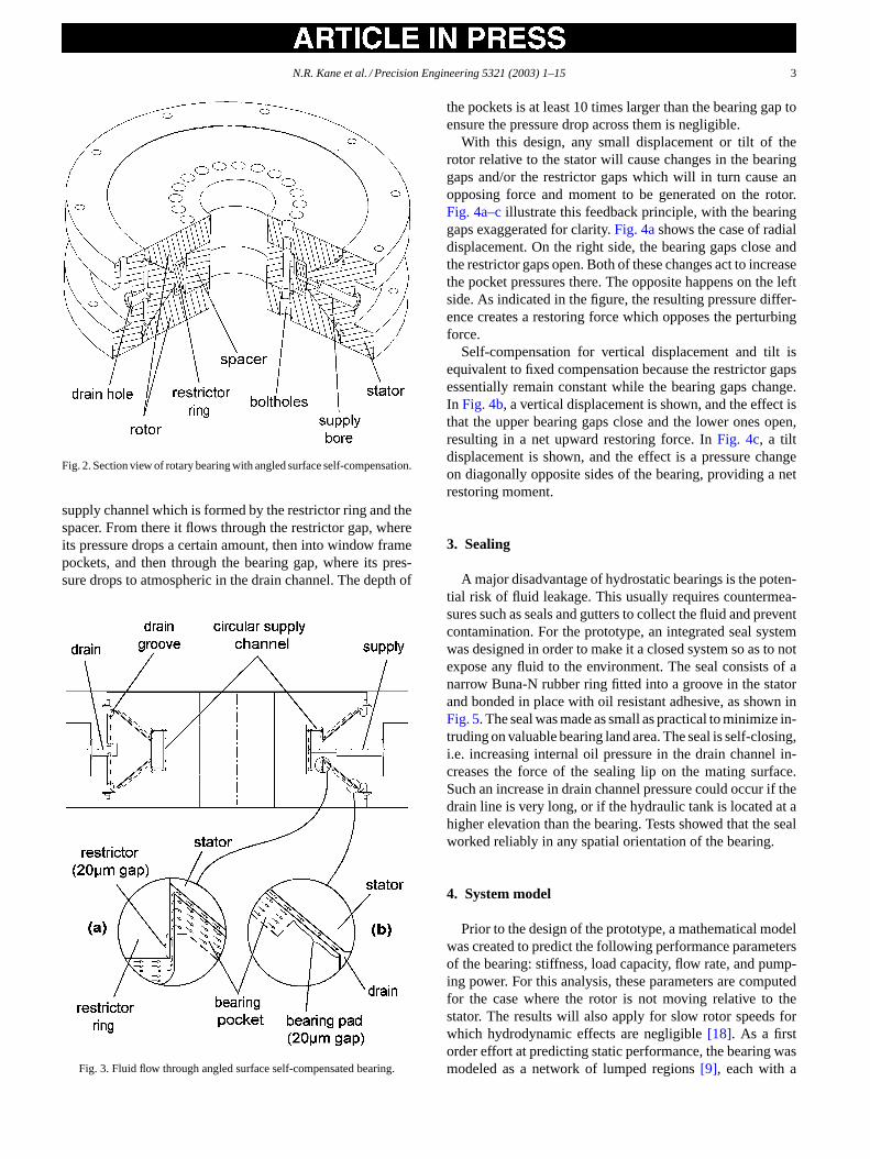
The bearing inFig. 1 comprises the stator, which is thelargest part; the restrictor ring, which is shrunk fit into thestator; the rotor, which consists of two geometrically identicalpieces that contain 20 bearing pockets, each 0.5 ± 0.2 mmdeep; and the spacer which aligns and connects the two halvesof the rotor.Fig. 2 shows a cross section of the assembly.Although it cannot be seen in the figure, the dimensions of theparts are chosen so that after assembly, a nominal restrictorand bearing land gap of 20�m is present between the rotorand the stator.

It should be noted that for this design to function prop-erly, the acute edge on each rotor half must be left sharpafter grinding—otherwise the pockets will be shorted to oneanother and radial and tilt stiffness will be nearly zero. There-fore, the rotor halves must be handled with care after they areground so that the acute edge remains sharp and unharmed.

Fig. 3 illustrates the fluid flow path through the bearing.The small arrows indicate the flow direction of the fluid dur-ing operation. After entering the bearing through the supplyhole on the right side, the pressurized fluid fills the annular

N.R. Kane et al. / Precision Engineering 5321 (2003) 1–15 3

Fig. 2. Section view of rotary bearing with angled surface self-compensation.

supply channel which is formed by the restrictor ring and thespacer. From there it flows through the restrictor gap, whereits pressure drops a certain amount, then into window framepockets, and then through the bearing gap, where its pres-sure drops to atmospheric in the drain channel. The depth of

Fig. 3. Fluid flow through angled surface self-compensated bearing.

the pockets is at least 10 times larger than the bearing gap toensure the pressure drop across them is negligible.

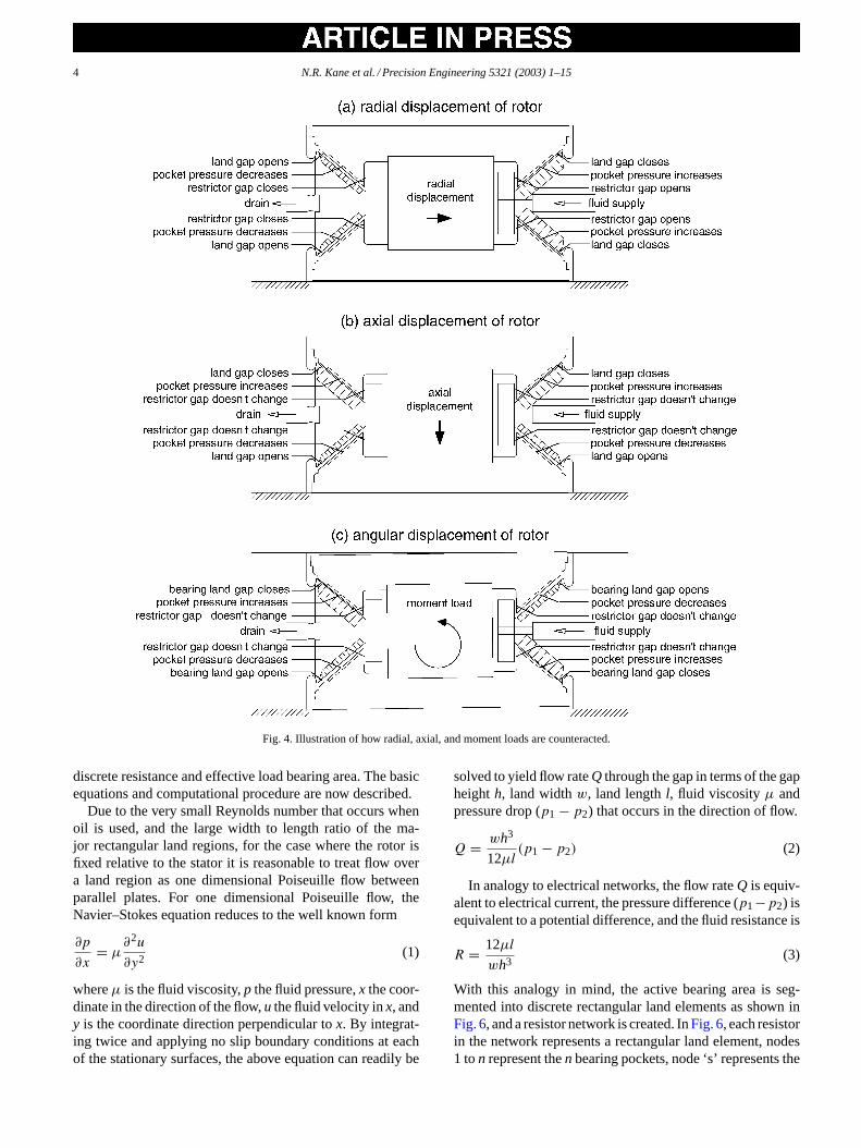
With this design, any small displacement or tilt of therotor relative to the stator will cause changes in the bearinggaps and/or the restrictor gaps which will in turn cause anopposing force and moment to be generated on the rotor.Fig. 4a–cillustrate this feedback principle, with the bearinggaps exaggerated for clarity.Fig. 4ashows the case of radialdisplacement. On the right side, the bearing gaps close andthe restrictor gaps open. Both of these changes act to increasethe pocket pressures there. The opposite happens on the leftside. As indicated in the figure, the resulting pressure differ-ence creates a restoring force which opposes the perturbingforce.

Self-compensation for vertical displacement and tilt isequivalent to fixed compensation because the restrictor gapsessentially remain constant while the bearing gaps change.In Fig. 4b, a vertical displacement is shown, and the effect isthat the upper bearing gaps close and the lower ones open,resulting in a net upward restoring force. InFig. 4c, a tiltdisplacement is shown, and the effect is a pressure changeon diagonally opposite sides of the bearing, providing a netrestoring moment.

3. Sealing

A major disadvantage of hydrostatic bearings is the poten-tial risk of fluid leakage. This usually requires countermea-sures such as seals and gutters to collect the fluid and preventcontamination. For the prototype, an integrated seal systemwas designed in order to make it a closed system so as to notexpose any fluid to the environment. The seal consists of anarrow Buna-N rubber ring fitted into a groove in the statorand bonded in place with oil resistant adhesive, as shown inFig. 5. The seal was made as small as practical to minimize in-truding on valuable bearing land area. The seal is self-closing,i.e. increasing internal oil pressure in the drain channel in-creases the force of the sealing lip on the mating surface.Such an increase in drain channel pressure could occur if thedrain line is very long, or if the hydraulic tank is located at ahigher elevation than the bearing. Tests showed that the sealworked reliably in any spatial orientation of the bearing.

4. System model

Prior to the design of the prototype, a mathematical modelwas created to predict the following performance parametersof the bearing: stiffness, load capacity, flow rate, and pump-ing power. For this analysis, these parameters are computedfor the case where the rotor is not moving relative to thestator. The results will also apply for slow rotor speeds forwhich hydrodynamic effects are negligible[18]. As a firstorder effort at predicting static performance, the bearing wasmodeled as a network of lumped regions[9], each with a


Fig. 4. Illustration of how radial, axial, and moment loads are counteracted.

discrete resistance and effective load bearing area. The basicequations and computational procedure are now described.

Due to the very small Reynolds number that occurs whenoil is used, and the large width to length ratio of the ma-jor rectangular land regions, for the case where the rotor isfixed relative to the stator it is reasonable to treat flow overa land region as one dimensional Poiseuille flow betweenparallel plates. For one dimensional Poiseuille flow, theNavier–Stokes equation reduces to the well known form

∂p

∂x= µ

∂2u

∂y2(1)

whereµ is the fluid viscosity,p the fluid pressure,x the coor-dinate in the direction of the flow,u the fluid velocity inx, andy is the coordinate direction perpendicular tox. By integrat-ing twice and applying no slip boundary conditions at eachof the stationary surfaces, the above equation can readily be

solved to yield flow rateQ through the gap in terms of the gapheighth, land widthw, land lengthl, fluid viscosityµ andpressure drop (p1 − p2) that occurs in the direction of flow.

Q = wh3

12µl(p1 − p2) (2)

In analogy to electrical networks, the flow rateQ is equiv-alent to electrical current, the pressure difference (p1−p2) isequivalent to a potential difference, and the fluid resistance is

R = 12µl

wh3(3)

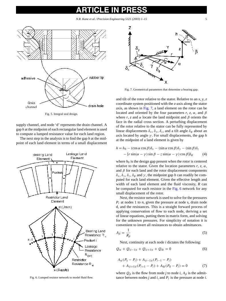
With this analogy in mind, the active bearing area is seg-mented into discrete rectangular land elements as shown inFig. 6, and a resistor network is created. InFig. 6, each resistorin the network represents a rectangular land element, nodes1 ton represent then bearing pockets, node ‘s’ represents the


Fig. 5. Integral seal design.

supply channel, and node ‘d’ represents the drain channel. Agaph at the midpoint of each rectangular land element is usedto compute a lumped resistance value for each land region.

The next step in the analysis is to find the gaph at the mid-point of each land element in terms of a small displacement

Fig. 6. Lumped resistor network to model fluid flow.

Fig. 7. Geometrical parameters that determine a bearing gap.

and tilt of the rotor relative to the stator. Relative to anx, y, zcoordinate system positioned with thez-axis along the statoraxis, as shown inFig. 7, a land element on the rotor can belocated and oriented by the four parametersr, z, α, andβ

wherer, z andα locate the land midpoint andβ orients theface in the radial cross section. A perturbing displacementof the rotor relative to the stator can be fully represented bylinear displacementsδx , δy , δz, and a tilt angleδφ about anaxis located by angleγ . For small displacements, the gaphat the midpoint of a land element is given by

h= h0 − (cosα cosβ)δx − (sinα cosβ)δy − (sinβ)δz

− [r sin(α − γ ) sinβ − z sin(α − γ ) cosβ]δφ (4)

whereh0 is the design gap present when the rotor is centeredrelative to the stator. Given the location parametersr, z, α,andβ for each land and the rotor displacement componentsδx , δy , δz, δφ andγ , the midpoint gaph can readily be com-puted for each land element. Given the effective length andwidth of each land element and the fluid viscosity,R canbe computed for each resistor in theFig. 6 network for anysmall displacement of the rotor.

Next, the resistor network is used to solve for the pressuresPi at nodes 1 ton, given the pressure at node s, drain noded, and the resistances. This is a straight forward process ofapplying conservation of flow to each node, deriving a setof linear equations, putting them in matrix form, and solvingfor the unknown pressures. For simplicity of notation it isconvenient to invert all resistances to obtain admittances.

Aji = 1

Rji(5)

Next, continuity at each nodei dictates the following:

Qsi + Q(i−1)i + Q(i+1)i + Qdi = 0 (6)

Asi (Ps − Pi) + A(i−1)i (Pi−1 − Pi)

+ A(i+1)i (Pi+1 − Pi) + Adi (Pd − Pi) = 0 (7)

whereQji is the flow from nodej to nodei, Aji is the admit-tance between nodesj andi, andPi is the pressure at nodei.


The above indexes are cyclical, meaning that an index equalto 0 should be replaced withn, and an index equal ton + 1should be replaced with 1. Setting the drain node pressurePdto 0 and rearranging yields

A(i−1)iPi−1 + (−Asi − A(i−1)i − A(i+1)i − Adi )Pi

+ A(i+1)iPi+1 = −AsiPs (8)

Eq. (8)can be put in matrix form whereP is a vector of theunknown node pressuresPi , andB is a constant vector.

[Z]P = B (9)

Bi = −AsiPs (10)

The non-zero terms of [Z] are the coefficients of thePi valuesin Eq. (8):

Zi(i−1) = A(i−1)i (11)

Zii = −Asi − A(i−1)i − Ai(i+1) − Adi (12)

Zi(i+1) = Ai(i+1) (13)

The vectorPPP is readily found from

P = [Z]−1B (14)

The next step is to use the pocket pressures to compute theflow rate into the bearing. The flow rate out of the bearing,which by continuity is equal to the flow into the bearing, isreadily computed from the bearing land admittances as

Q =n∑

i=1

AdiPi (15)

The pumping powerW is

W = PsQ (16)

The next step is to use the pocket pressures to compute thenet force and moment on the rotor. For each rectangular landelement, the normal forceFl is given by

Fl = 12wlPa + 1

2wlPb (17)

wherew and l are the land width and length, respectively,andPa andPb are the pressures present on opposite edges ofthe land. The normal forceFp on each pocket is given by

Fp = wplpPi (18)

wherewp is the pocket width,lp is the pocket length, andPi

is the pocket pressure. The force and moment exerted on therotor by a land element or a pocket element is given by

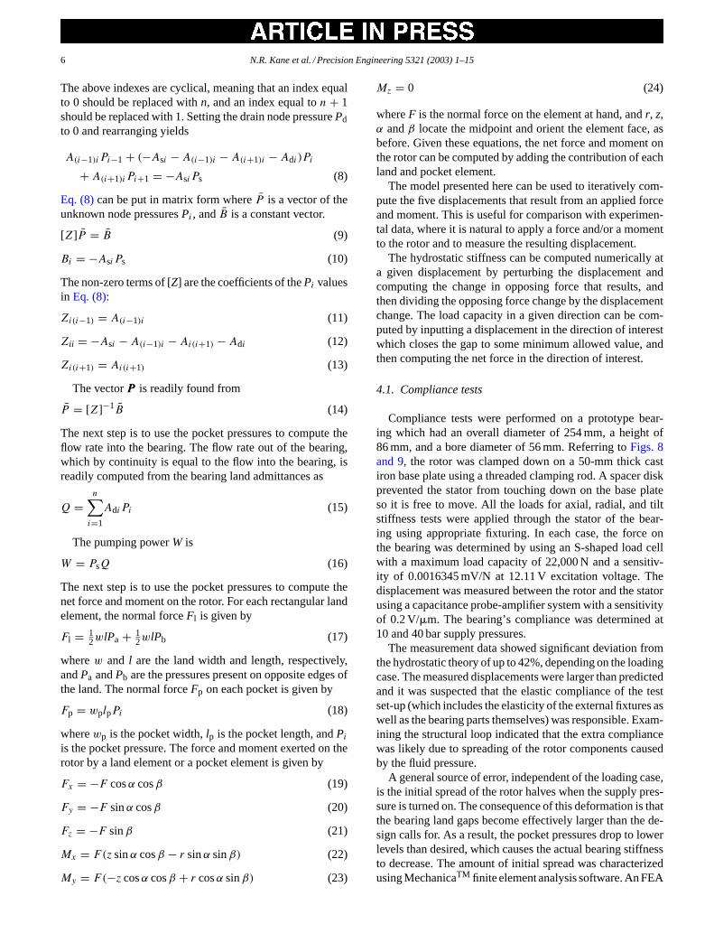
Fx = −F cosα cosβ (19)

Fy = −F sinα cosβ (20)

Fz = −F sinβ (21)

Mx = F(z sinα cosβ − r sinα sinβ) (22)

My = F(−z cosα cosβ + r cosα sinβ) (23)

Mz = 0 (24)

whereF is the normal force on the element at hand, andr, z,α andβ locate the midpoint and orient the element face, asbefore. Given these equations, the net force and moment onthe rotor can be computed by adding the contribution of eachland and pocket element.

The model presented here can be used to iteratively com-pute the five displacements that result from an applied forceand moment. This is useful for comparison with experimen-tal data, where it is natural to apply a force and/or a momentto the rotor and to measure the resulting displacement.

The hydrostatic stiffness can be computed numerically ata given displacement by perturbing the displacement andcomputing the change in opposing force that results, andthen dividing the opposing force change by the displacementchange. The load capacity in a given direction can be com-puted by inputting a displacement in the direction of interestwhich closes the gap to some minimum allowed value, andthen computing the net force in the direction of interest.

4.1. Compliance tests

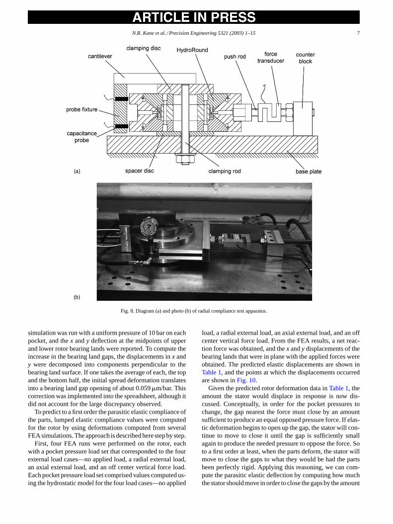
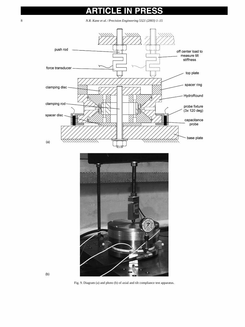
Compliance tests were performed on a prototype bear-ing which had an overall diameter of 254 mm, a height of86 mm, and a bore diameter of 56 mm. Referring toFigs. 8and 9, the rotor was clamped down on a 50-mm thick castiron base plate using a threaded clamping rod. A spacer diskprevented the stator from touching down on the base plateso it is free to move. All the loads for axial, radial, and tiltstiffness tests were applied through the stator of the bear-ing using appropriate fixturing. In each case, the force onthe bearing was determined by using an S-shaped load cellwith a maximum load capacity of 22,000 N and a sensitiv-ity of 0.0016345 mV/N at 12.11 V excitation voltage. Thedisplacement was measured between the rotor and the statorusing a capacitance probe-amplifier system with a sensitivityof 0.2 V/�m. The bearing’s compliance was determined at10 and 40 bar supply pressures.

The measurement data showed significant deviation fromthe hydrostatic theory of up to 42%, depending on the loadingcase. The measured displacements were larger than predictedand it was suspected that the elastic compliance of the testset-up (which includes the elasticity of the external fixtures aswell as the bearing parts themselves) was responsible. Exam-ining the structural loop indicated that the extra compliancewas likely due to spreading of the rotor components causedby the fluid pressure.

A general source of error, independent of the loading case,is the initial spread of the rotor halves when the supply pres-sure is turned on. The consequence of this deformation is thatthe bearing land gaps become effectively larger than the de-sign calls for. As a result, the pocket pressures drop to lowerlevels than desired, which causes the actual bearing stiffnessto decrease. The amount of initial spread was characterizedusing MechanicaTM finite element analysis software. An FEA


Fig. 8. Diagram (a) and photo (b) of radial compliance test apparatus.

simulation was run with a uniform pressure of 10 bar on eachpocket, and thex andy deflection at the midpoints of upperand lower rotor bearing lands were reported. To compute theincrease in the bearing land gaps, the displacements inx andy were decomposed into components perpendicular to thebearing land surface. If one takes the average of each, the topand the bottom half, the initial spread deformation translatesinto a bearing land gap opening of about 0.059�m/bar. Thiscorrection was implemented into the spreadsheet, although itdid not account for the large discrepancy observed.

To predict to a first order the parasitic elastic compliance ofthe parts, lumped elastic compliance values were computedfor the rotor by using deformations computed from severalFEA simulations. The approach is described here step by step.

First, four FEA runs were performed on the rotor, eachwith a pocket pressure load set that corresponded to the fourexternal load cases—no applied load, a radial external load,an axial external load, and an off center vertical force load.Each pocket pressure load set comprised values computed us-ing the hydrostatic model for the four load cases—no applied

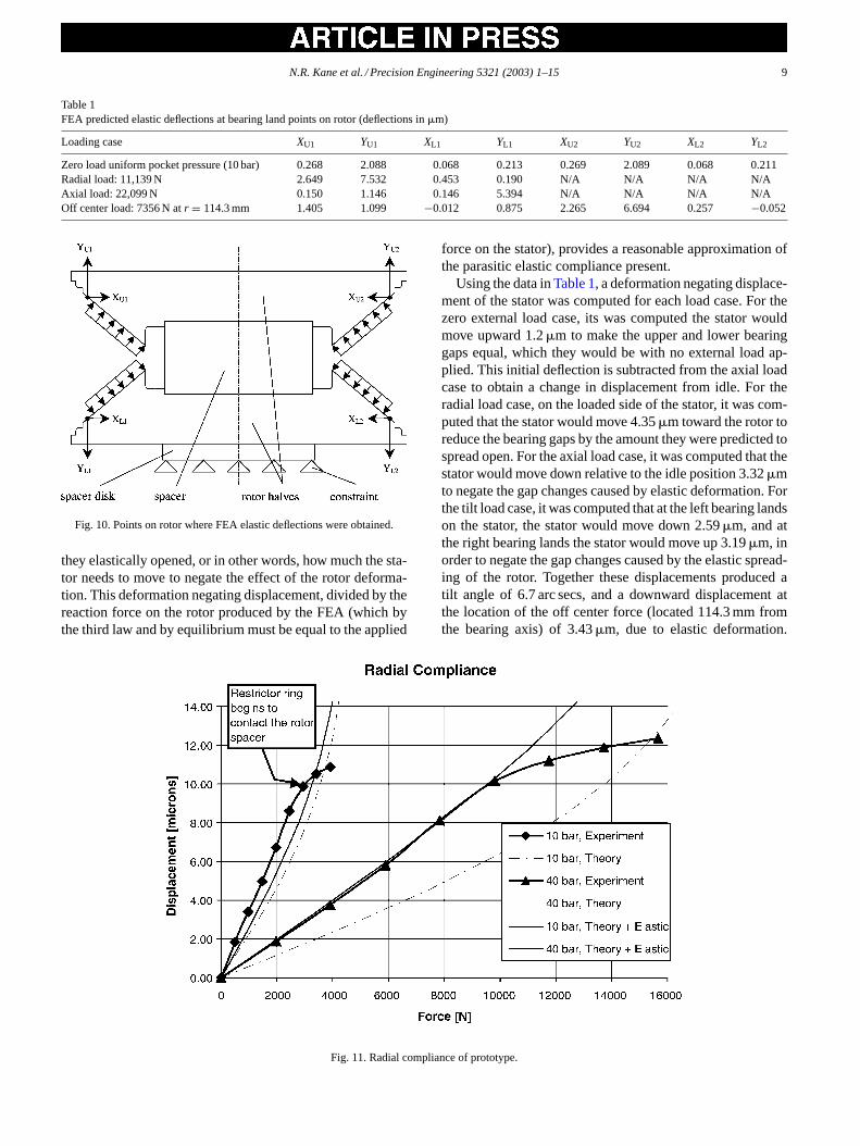
load, a radial external load, an axial external load, and an offcenter vertical force load. From the FEA results, a net reac-tion force was obtained, and thex andy displacements of thebearing lands that were in plane with the applied forces wereobtained. The predicted elastic displacements are shown inTable 1, and the points at which the displacements occurredare shown inFig. 10.

Given the predicted rotor deformation data inTable 1, theamount the stator would displace in response is now dis-cussed. Conceptually, in order for the pocket pressures tochange, the gap nearest the force must close by an amountsufficient to produce an equal opposed pressure force. If elas-tic deformation begins to open up the gap, the stator will con-tinue to move to close it until the gap is sufficiently smallagain to produce the needed pressure to oppose the force. Soto a first order at least, when the parts deform, the stator willmove to close the gaps to what they would be had the partsbeen perfectly rigid. Applying this reasoning, we can com-pute the parasitic elastic deflection by computing how muchthe stator should move in order to close the gaps by the amount


Fig. 9. Diagram (a) and photo (b) of axial and tilt compliance test apparatus.


Table 1FEA predicted elastic deflections at bearing land points on rotor (deflections in�m)

Loading case XU1 YU1 XL1 YL1 XU2 YU2 XL2 YL2

Zero load uniform pocket pressure (10 bar) 0.268 2.088 0.068 0.213 0.269 2.089 0.068 0.211Radial load: 11,139 N 2.649 7.532 0.453 0.190 N/A N/A N/A N/AAxial load: 22,099 N 0.150 1.146 0.146 5.394 N/A N/A N/A N/AOff center load: 7356 N atr = 114.3 mm 1.405 1.099 −0.012 0.875 2.265 6.694 0.257 −0.052

Fig. 10. Points on rotor where FEA elastic deflections were obtained.

they elastically opened, or in other words, how much the sta-tor needs to move to negate the effect of the rotor deforma-tion. This deformation negating displacement, divided by thereaction force on the rotor produced by the FEA (which bythe third law and by equilibrium must be equal to the applied

Fig. 11. Radial compliance of prototype.

force on the stator), provides a reasonable approximation ofthe parasitic elastic compliance present.

Using the data inTable 1, a deformation negating displace-ment of the stator was computed for each load case. For thezero external load case, its was computed the stator wouldmove upward 1.2�m to make the upper and lower bearinggaps equal, which they would be with no external load ap-plied. This initial deflection is subtracted from the axial loadcase to obtain a change in displacement from idle. For theradial load case, on the loaded side of the stator, it was com-puted that the stator would move 4.35�m toward the rotor toreduce the bearing gaps by the amount they were predicted tospread open. For the axial load case, it was computed that thestator would move down relative to the idle position 3.32�mto negate the gap changes caused by elastic deformation. Forthe tilt load case, it was computed that at the left bearing landson the stator, the stator would move down 2.59�m, and atthe right bearing lands the stator would move up 3.19�m, inorder to negate the gap changes caused by the elastic spread-ing of the rotor. Together these displacements produced atilt angle of 6.7 arc secs, and a downward displacement atthe location of the off center force (located 114.3 mm fromthe bearing axis) of 3.43�m, due to elastic deformation.


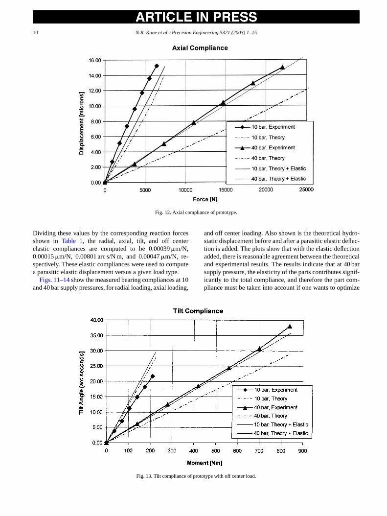
Fig. 12. Axial compliance of prototype.

Dividing these values by the corresponding reaction forcesshown in Table 1, the radial, axial, tilt, and off centerelastic compliances are computed to be 0.00039�m/N,0.00015�m/N, 0.00801 arc s/N m, and 0.00047�m/N, re-spectively. These elastic compliances were used to computea parasitic elastic displacement versus a given load type.

Figs. 11–14show the measured bearing compliances at 10and 40 bar supply pressures, for radial loading, axial loading,

Fig. 13. Tilt compliance of prototype with off center load.

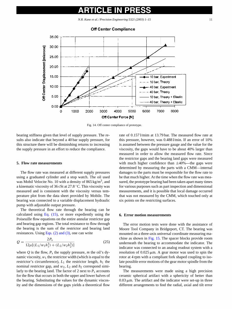
and off center loading. Also shown is the theoretical hydro-static displacement before and after a parasitic elastic deflec-tion is added. The plots show that with the elastic deflectionadded, there is reasonable agreement between the theoreticaland experimental results. The results indicate that at 40 barsupply pressure, the elasticity of the parts contributes signif-icantly to the total compliance, and therefore the part com-pliance must be taken into account if one wants to optimize


Fig. 14. Off center compliance of prototype.

bearing stiffness given that level of supply pressure. The re-sults also indicate that beyond a 40 bar supply pressure, forthis structure there will be diminishing returns to increasingthe supply pressure in an effort to reduce the compliance.

5. Flow rate measurements

The flow rate was measured at different supply pressuresusing a graduated cylinder and a stop watch. The oil usedwas Mobil Velocite No. 10 with a density of 865 kg/m3, anda kinematic viscosity of 36 cSt at 27.8◦C. This viscosity wasmeasured and is consistent with the viscosity versus tem-perature plot from the data sheet provided by Mobile. Thebearing was connected to a variable displacement hydraulicpump with adjustable output pressure.

The theoretical flow rate through the bearing can becalculated usingEq. (15), or more expediently using thePoiseuille flow equations on the entire annular restrictor gapand bearing gap regions. The total resistance to flow throughthe bearing is the sum of the restrictor and bearing landresistances. UsingEqs. (2) and (3), one can write

Q = 2Ps

12µ[(L1/w1h31) + (L2/w2h

32)]

(25)

whereQ is the flow,Ps the supply pressure,m the oil’s dy-namic viscosity,w1 the restrictor width (which is equal to therestrictor’s circumference),L1 the restrictor length,h1 thenominal restrictor gap, andw2, L2 andh2 correspond simi-larly to the bearing land. The factor of 2 next toPs accountsfor the flow that occurs in both the upper and lower halves ofthe bearing. Substituting the values for the dynamic viscos-ity and the dimensions of the gaps yields a theoretical flow

rate of 0.157 l/mim at 13.79 bar. The measured flow rate atthis pressure, however, was 0.488 l/min. If an error of 10%is assumed between the pressure gauge and the value for theviscosity, the gaps would have to be about 40% larger thanmeasured in order to allow the measured flow rate. Sincethe restrictor gaps and the bearing land gaps were measuredwith much higher confidence than±40%—the gaps weredetermined by measuring the parts with a CMM—internaldamages to the parts must be responsible for the flow rate tobe that much higher. At the time when the flow rate was mea-sured, the prototype bearing had been taken apart many timesfor various purposes such as part inspection and dimensionalmeasurements, and it is possible that local damage occurredthat was not measured by the CMM, which touched only atsix points on the restricting surfaces.

6. Error motion measurements

The error motion tests were done with the assistance ofMoore Tool Company in Bridgeport, CT. The bearing wasmounted on a three-axis universal coordinate measuring ma-chine as shown inFig. 15. The spacer blocks provide roomunderneath the bearing to accommodate the indicator. Theindicator was connected to an analog readout system with aresolution of 0.025�m. A gear motor was used to spin therotor at 4 rpm with a compliant fork shaped coupling to iso-late possible error motions of the gear motor spindle from thebearing.

The measurements were made using a high precisionceramic spherical artifact with a sphericity of better than0.03�m. The artifact and the indicator were set-up in threedifferent arrangements to find the radial, axial and tilt error


Fig. 15. Diagram (a) and photo (b) of error motion set-up.

motions. The first measurement was done to determine thepure radial error motion with the artifact located in the radialand axial center of the bearing and an indicator pointingto the equator of the precision sphere (see position A inFig. 15a). Note that since the artifact was so spherical andthe bearing was not expected to be so good, a DonaldsonReversal Test[20] was not done when the measurements

were carried out, and hence strictly speaking, runout mea-surements were made; however, again, because the artifactwas so accurate, the error motion is at least as good as therunout, and hence, here we will use the term “error motion”.

The axial error motion was measured by positioning theindicator tip on the very bottom center point of the precisionsphere (see position B inFig. 15a). Radial error motions dur-ing the measurement of the axial error motion will have acosine error effect and therefore have only a negligible influ-ence on the axial error motion.

Fig. 16. Polar plot of the (a) radial error motion and (b) axial error motion(1 division= 0.127�m, the radial and axial error motions are approximately0.05�m).


Table 2Error motion summary table

Radial runout (�m) <0.05Axial runout (�m) <0.05Tilt error motion (arc s) 0.09Part accuracy (�m) 2.5Averaging factor 50

The test showed very good results as shown in the polarplot inFig. 16a and b. The scale on both plots is 0.127�m perdivision, which means that each one of the circles for axialand radial error motion lies within approximately 50 nm.

The tilt error motion was estimated by computing themaximum difference that occurred between the error motionmeasured at positions A and C, and then dividing by thedistance between A and C. This yields a maximum tilt errorof about 0.09 arc s.Table 2 summarizes the error motionmeasurement results.

7. Part accuracy versus error motion

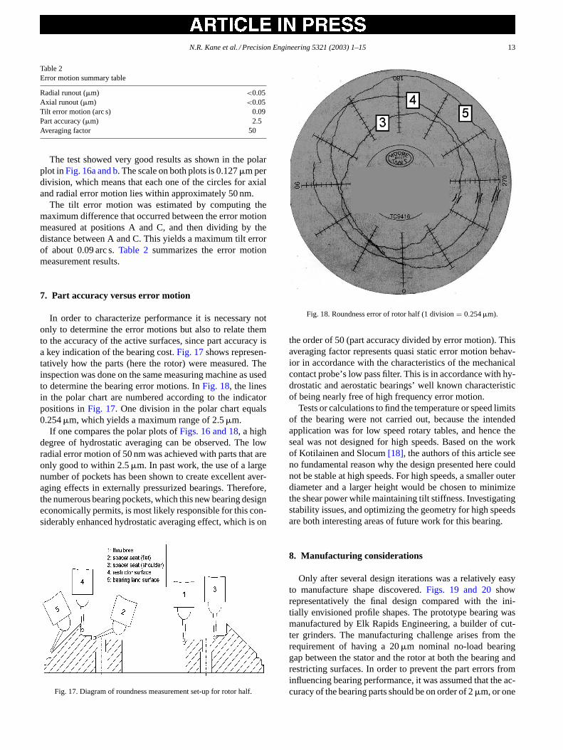
In order to characterize performance it is necessary notonly to determine the error motions but also to relate themto the accuracy of the active surfaces, since part accuracy isa key indication of the bearing cost.Fig. 17shows represen-tatively how the parts (here the rotor) were measured. Theinspection was done on the same measuring machine as usedto determine the bearing error motions. InFig. 18, the linesin the polar chart are numbered according to the indicatorpositions inFig. 17. One division in the polar chart equals0.254�m, which yields a maximum range of 2.5�m.

If one compares the polar plots ofFigs. 16 and 18, a highdegree of hydrostatic averaging can be observed. The lowradial error motion of 50 nm was achieved with parts that areonly good to within 2.5�m. In past work, the use of a largenumber of pockets has been shown to create excellent aver-aging effects in externally pressurized bearings. Therefore,the numerous bearing pockets, which this new bearing designeconomically permits, is most likely responsible for this con-siderably enhanced hydrostatic averaging effect, which is on

Fig. 17. Diagram of roundness measurement set-up for rotor half.

Fig. 18. Roundness error of rotor half (1 division= 0.254�m).

the order of 50 (part accuracy divided by error motion). Thisaveraging factor represents quasi static error motion behav-ior in accordance with the characteristics of the mechanicalcontact probe’s low pass filter. This is in accordance with hy-drostatic and aerostatic bearings’ well known characteristicof being nearly free of high frequency error motion.

Tests or calculations to find the temperature or speed limitsof the bearing were not carried out, because the intendedapplication was for low speed rotary tables, and hence theseal was not designed for high speeds. Based on the workof Kotilainen and Slocum[18], the authors of this article seeno fundamental reason why the design presented here couldnot be stable at high speeds. For high speeds, a smaller outerdiameter and a larger height would be chosen to minimizethe shear power while maintaining tilt stiffness. Investigatingstability issues, and optimizing the geometry for high speedsare both interesting areas of future work for this bearing.

8. Manufacturing considerations

Only after several design iterations was a relatively easyto manufacture shape discovered.Figs. 19 and 20showrepresentatively the final design compared with the ini-tially envisioned profile shapes. The prototype bearing wasmanufactured by Elk Rapids Engineering, a builder of cut-ter grinders. The manufacturing challenge arises from therequirement of having a 20�m nominal no-load bearinggap between the stator and the rotor at both the bearing andrestricting surfaces. In order to prevent the part errors frominfluencing bearing performance, it was assumed that the ac-curacy of the bearing parts should be on order of 2�m, or one


Fig. 19. Initial stator design (left) and the final design (right).

Fig. 20. Initial rotor design (left) and the final design (right).

order of magnitude less than the nominal bearing gap. Froma machinist’s point of view, the design changes inFigs. 19and 20represent major improvements. InFig. 19, the statoris initially cut out of one piece with a radius at the neck of thehammerhead shape. This requires a profiled grinding wheelwhich causes many problems in terms of placing the radiuswithin 2�m and matching it to its counterpart on the rotor.

In the new design for the stator, the “hammer head” shapeis added as a separate ring—the restrictor ring as shown inFig. 1. Thus, a radius is avoided and a profiled grinding wheelis no longer needed. All the precision surfaces are straightand can be ground with straight grinding wheels. Addition-ally, the upper and lower restrictor surfaces will be veryprecisely concentric because they are part of a single ringsurface.

Similar considerations apply to the rotor. The problem withthe initial design is that some precision surfaces are hidden ina groove and therefore they are difficult to reach with grind-ing or measuring equipment.Fig. 20shows the improved fi-nal design next to the initial design. Straight grinding wheelscan be used here as well and the precision surfaces are easilyaccessible. Furthermore, in order to match the angular sur-faces of the stator and the rotor, the parts are ground in thesame set-up. Also, the bearing gap can be accurately set with

minimal machining by grinding down or adding a shim tothe spacer.

A minor potential drawback to this design is the sharpacute knife edges, which need to be sharp to block a poten-tial short circuit between bearing pockets. A short circuitchannel would not allow pocket pressures to be differentfrom one another, which would virtually eliminate the radialand tilt stiffness of the bearing. Therefore, the knife edgesrequire careful attention during the manufacturing and as-sembly process. However, once the bearing is assembled,the knife edges are completely protected from damage andhence pose no problems during operation.

9. Conclusions

A novel hydrostatic bearing has been presented whichis potentially useful for applications that require very highrotational precision and stiffness in a low profile package.The relatively high averaging factor allows bearing part tol-erances on the order of 50 times more generous than theintended bearing accuracy. This makes it possible to attainhigh accuracy of motion with relatively low cost parts. Addi-tional cost reduction is achieved by the fact that the bearing


does not need capillaries or orifices to be assembled or tunedfor operation, nor does it require special grooves or slotsthat must have a precise depth. Further work may investigatecasting the pockets into the rotors to lower the manufacturingcost.

A disadvantage that the presented bearing shares withevery other hydrostatic bearing is the need for an externalhydraulic power unit and return plumbing, which adds heatto the system and also adds extra cost. However, many ma-chining centers and other machine tools are already equippedwith a hydraulic unit to actuate work piece clamps or toolchangers. Since the oil consumption of the bearing is onlyabout 0.5 l/min at an operating pressure of 40 bar, only about35 W of power is dissipated. For applications that cannot tol-erate even the relatively small heat generation, a chiller canbe added to the hydraulic unit to remove heat from the oil.Future work will focus on the integration of this design intoexisting or new machine tool structures and to investigatethe benefits of high accuracy, stiffness, and damping duringactual machining operations.

Acknowledgments

This work was sponsored in part by the Defense LogisticsAgency (DLA) Manufacturing Technology Program andmanaged by the Naval Research Laboratory. The authorswould also like to thank Elk Rapids Engineering in ElkRapids, MI for manufacturing the prototype, and Moore Spe-cial Tool in Bridgeport, CT for performing metrology experi-ments. Thanks also to Jeff Roblee, Rob Koning, Fred Mispel,and Ben Hale from Precitech Inc. in Keene, NH for assistingwith part geometry and flow rate measurements. Nathan R.Kane was sponsored by the Fannie and John Hertz Founda-tion Fellowship. Joachim Sihler received funding from AlfingKessler Sondermaschinen, Wasseralfingen, Germany, andthe Studentenwerk Stuttgart of the University of Stuttgart,Stuttgart, Germany, for conducting this research work.

References

[1] Fuller DD. Theory and practice of lubrication for engineers, 2nd ed.New York: Wiley; 1984.

[2] Rowe W. Hydrostatic and hybrid bearing design. London: Butterworth;1983.

[3] Slocum AH. Precision machine design. Englewood Cliffs, NJ:Prentice-Hall; 1992.

[4] Weck M. Handbook of machine tools. Chichester (West Sussex), NewYork: Wiley; 1984.

[5] Hoffer FW. Automatic fluid pressure balancing system. US Patent2,449,297 (September 1948).

[6] Arneson HEG. Hydrostatic bearing structure. US Patent 3,305,282(February 1967).

[7] Arneson HEG. Externally pressurized bearing structure. US Patent3,472,565 (October 1969).

[8] Hedberg OJG. Movable machine element supported with the aid of agas or fluid bearing. US Patent 3,754,799 (August 1973).

[9] Velednitski VM, Push VE, Schimanovich MA. Static load characteris-tics of a hydrostatic radial bearing without draining grooves and withopposed acting restrictors. Mach Tool 1980;51(10):8–11.

[10] Slocum AH. Self-compensating hydrostatic linear motion bearing. USPatent 5,104,237 (14 April 1992).

[11] Slocum AH, Scagnetti PE, Kane NR, Brünnner C. Design of self-compensated water-hydrostatic bearings. Prec Eng 1995;17(3):173–85.

[12] Zeleny J. Servostatic guideways—a new kind of hydraulically operatingguideways for machine tools. In: Proceedings of the 10th InternationalMach. Tool Des. Res. Conference, September 1969.

[13] Tsumaki N, Tokisue H, Inoue H. Guiding apparatus. US Patent4,630,942 (December 1986).

[14] Marathe SM, Cuppan BC, Ehrhardt OW, Scherer JC, Schmitz TE. Ser-vostatic bearing system with variable stiffness. US Patent 4,080,009(March 1978).

[15] Tully N. Static and dynamic performance of an infinite stiffness hydro-static bearing. ASME Trans J Lubr Technol 1977;99:106–12.

[16] Wasson SK. Low profile self-compensated hydrostatic thrust bearing.US Patent 5,533,814 (July 1996).

[17] Wasson KL, Slocum AH. Integrated shaft self-compensating hydro-static bearing. US Patent 5,700,092 (23 December 1997).

[18] Kotilainen M, Slocum A. Manufacturing of cast monolithic hydrostaticjournal bearings. J Int Soc Prec Eng Nanotechnol 2001;25:235–44.

[19] Kane N, Slocum A. Modular hydrostatic bearing with carriage form fitto profile rail. US Patent 5,971,614 (October 1999).

[20] ANSI Standard B89.3.4M-1985. Axis of Rotation: Methods for Spec-ifying and Testing.

a hydrostatic rotary bearing with angled surface self...

Documents