a java based interactive control design and …
TRANSCRIPT

A JAVA BASED INTERACTIVE CONTROL DESIGN
AND TUNING PLATFORM
AARON RADKE
Bachelor of Science in Electrical Engineering
Cleveland State University
May, 2002
Bachelor of Arts in Physics
Cleveland State University
May, 2002
submitted in partial fulfillment of the requirements for the degree
MASTERS OF ENGINEERING
at the
CLEVELAND STATE UNIVERSITY
July 2003

This thesis has been approved for the
Department of ELECTRICAL AND COMPUTER ENGINEERING
and the College of Graduate Studies by
Thesis Committee Chairperson, Dr. Zhiqiang Gao
Department/Date
Dr. Yongjian Fu
Department/Date
Dr. Dan Simon
Department/Date

To my parents...

ACKNOWLEDGMENTS
First, I would like to express my deepest appreciation to my advisor, Dr.
Zhiqiang Gao, for his supervision and help throughout the course of my study. Most of
all, I am grateful for his vision and encouragement to continue in higher education and
research. I enjoy learning from his teaching philosphy and problem solving methods.
I am also grateful for his flexibility in the area and topics that interest me for research.
Jack Zeller has also been a great source of encouragement as an advisor with
sincere enthusiasm over all that I do.
I appreciate Dr. Dan Simon, Dr. Yongjian Fu, who are on my committee, for
their time in reading and evaluating this thesis.
I would also like to thank my fellow collegues and lab members: Rob Mik-
losovic, Weiwen Wang, Shahid Parvez, Bosheng Sun, Zhan Ping, Arthur Stachowicz,
Greg Tollis, Ivan Jurcic, Chunming Yang, Tong Ren, Frank Goeforth, Rachel Lim for
their guidance, help and encouragment in the research, writting and logistics. Adrian
Fox and Jan Bosch have also been a wonderful help by the great work done behind
the scenes, as well as the rest of the electrical engineering department for the endless
support given to me while at Cleveland State University.
I would also like to give a special thanks to Tina Miklosovic for her thorough
review, corrections, and suggestions.
Finally, I cordially thank my family for their continuous support, encourage-
ment, and heartfelt joy in all that I do.
iv
A JAVA BASED INTERACTIVE CONTROL DESIGN
AND TUNING PLATFORM
AARON RADKE
ABSTRACT
This research focuses on building an interactive graphical tuning application
framework for control systems. The objective is to create an environment for con-
troller design that simplifies the repetitive tuning of multiple parameters, allowing
rapid insight into the effects of the parameters on control system performance. This
is accomplished by creating a simulation package for controller tuning written in Java,
offering a cross platform and web-based solution. The tool kit has several advantages
over existing conventional simulation packages. Primarily, it provides the ability to
interactively vary parameters for optimal performance. It gives control engineers a
tool to help explain and explore conventional and advanced control designs and al-
gorithms. The tool kit also offers an alternative to Matlab for practicing engineers
from the design phase to practical implementation.
v

TABLE OF CONTENTS
Page
ACKNOWLEDGMENTS . . . . . . . . . . . . . . . . . . . . . . . . . . . . . iv
ABSTRACT . . . . . . . . . . . . . . . . . . . . . . . . . . . . . . . . . . . . v
LIST OF TABLES . . . . . . . . . . . . . . . . . . . . . . . . . . . . . . . . . x
LIST OF FIGURES . . . . . . . . . . . . . . . . . . . . . . . . . . . . . . . . xi
CHAPTER
I. INTRODUCTION . . . . . . . . . . . . . . . . . . . . . . . . . . . . . . . 1
1.1 Project Focus . . . . . . . . . . . . . . . . . . . . . . . . . . . . 1
1.2 Motivation of Research . . . . . . . . . . . . . . . . . . . . . . . 2
1.3 Existing Software Tools . . . . . . . . . . . . . . . . . . . . . . . 2
1.3.1 Matlab . . . . . . . . . . . . . . . . . . . . . . . . . . . . 3
1.3.2 SysQuake . . . . . . . . . . . . . . . . . . . . . . . . . . . 4
1.4 Proposed Approach . . . . . . . . . . . . . . . . . . . . . . . . . 6
1.4.1 Problem Formulation . . . . . . . . . . . . . . . . . . . . 6
1.4.2 Software Development Strategy . . . . . . . . . . . . . . . 7
1.5 Software Requirements and Specifications . . . . . . . . . . . . . 8
1.6 Thesis Organization . . . . . . . . . . . . . . . . . . . . . . . . . 9
PART I SOFTWARE STRUCTURE . . . . . . . . . . . . . . . . . . . . . . 10
II. STRUCTURAL IMPLEMENTATION . . . . . . . . . . . . . . . . . . . 11
2.1 Focus on Difference Equations . . . . . . . . . . . . . . . . . . . 12
2.2 Fundamental Building Blocks . . . . . . . . . . . . . . . . . . . . 12
2.2.1 Object Orientedness . . . . . . . . . . . . . . . . . . . . . 12
2.2.2 Class Inheritance Structure . . . . . . . . . . . . . . . . . 16
vi

2.2.3 Block Interconnection . . . . . . . . . . . . . . . . . . . . 16
2.3 GUI Development . . . . . . . . . . . . . . . . . . . . . . . . . . 17
III. DATA FLOW IMPLEMENTATION . . . . . . . . . . . . . . . . . . . . 19
3.1 Developer’s Viewpoint . . . . . . . . . . . . . . . . . . . . . . . . 20
3.1.1 Top-level Managing Class . . . . . . . . . . . . . . . . . . 20
3.1.2 Setting Up a Simulation . . . . . . . . . . . . . . . . . . . 23
3.1.3 Building Blocks . . . . . . . . . . . . . . . . . . . . . . . 23
3.2 User’s Viewpoint . . . . . . . . . . . . . . . . . . . . . . . . . . . 24
PART II SYSTEM FUNCTIONALITIES AND APPLICATION . . . . . . . 26
IV. DIFFERENTIAL EQUATION SOLVER . . . . . . . . . . . . . . . . . 27
4.1 Comparison of Ode Solvers . . . . . . . . . . . . . . . . . . . . . 28
4.1.1 Simple Example Problem for Comparisons . . . . . . . . . 28
4.2 Differential Equation Solver Engine . . . . . . . . . . . . . . . . 31
4.2.1 Specific Conversions from Continuous Form to Discrete . 32
4.2.2 General s to z Transform Matrices . . . . . . . . . . . . . 36
4.2.3 General z Transfer Function to Difference Equations . . . 38
V. CONTROLLER DESIGN AND IMPLEMENTATION . . . . . . . . . . 41
5.1 Parameterization . . . . . . . . . . . . . . . . . . . . . . . . . . . 42
5.2 Approximate PID . . . . . . . . . . . . . . . . . . . . . . . . . . 42
5.3 Nonlinear PID . . . . . . . . . . . . . . . . . . . . . . . . . . . . 44
5.4 Active Disturbance Rejection Control . . . . . . . . . . . . . . . 46
5.5 Discrete Time Optimal Control . . . . . . . . . . . . . . . . . . . 48
5.6 Filters . . . . . . . . . . . . . . . . . . . . . . . . . . . . . . . . . 51
5.6.1 Pre-filters and Profiles . . . . . . . . . . . . . . . . . . . . 51
5.6.2 General Normalized Butterworth Filters . . . . . . . . . . 56
VI. A GENERAL MODEL DIAGRAM . . . . . . . . . . . . . . . . . . . . 60
vii

6.1 Classic System . . . . . . . . . . . . . . . . . . . . . . . . . . . . 61
6.2 Combined General System . . . . . . . . . . . . . . . . . . . . . 62
6.3 General Blocks . . . . . . . . . . . . . . . . . . . . . . . . . . . . 62
VII. ACTIVE OPTIMIZATION CONTROL . . . . . . . . . . . . . . . . . 66
7.1 Threshold Limit Requirement . . . . . . . . . . . . . . . . . . . . 66
7.1.1 Noise Level Limit . . . . . . . . . . . . . . . . . . . . . . 67
7.1.2 Rate of Change Limit . . . . . . . . . . . . . . . . . . . . 68
7.1.3 Overshoot Limit . . . . . . . . . . . . . . . . . . . . . . . 69
7.1.4 The Most Significant Bandwidth Threshold . . . . . . . . 69
7.2 Optimization and Threshold Assumptions . . . . . . . . . . . . . 69
7.3 Active Noise Quantification Methods . . . . . . . . . . . . . . . . 70
7.3.1 Max and Min . . . . . . . . . . . . . . . . . . . . . . . . . 71
7.3.2 Moving Average Window . . . . . . . . . . . . . . . . . . 72
7.3.3 Variance and Standard Deviation . . . . . . . . . . . . . . 73
7.3.4 Linear Regression . . . . . . . . . . . . . . . . . . . . . . 75
7.3.5 High-Pass Filter With Variance . . . . . . . . . . . . . . . 76
7.3.6 Wavelet for a New Variance Definition . . . . . . . . . . . 77
VIII. SUMMARY AND FUTURE RESEARCH . . . . . . . . . . . . . . . . 78
8.1 Summary . . . . . . . . . . . . . . . . . . . . . . . . . . . . . . . 79
8.1.1 Simulation Building Blocks . . . . . . . . . . . . . . . . . 80
8.1.2 Simple GUI Examples . . . . . . . . . . . . . . . . . . . . 81
8.2 Future Research . . . . . . . . . . . . . . . . . . . . . . . . . . . 81
8.2.1 Additional Library Blocks . . . . . . . . . . . . . . . . . . 81
8.2.2 Graphical Setup of SimBlocks . . . . . . . . . . . . . . . 82
8.2.3 Extension to a Hardware Tuning and Monitoring Interface 83
viii

8.2.4 Extension to Automated Computer Assisted Design for
Controls . . . . . . . . . . . . . . . . . . . . . . . . . . . 83
BIBLIOGRAPHY . . . . . . . . . . . . . . . . . . . . . . . . . . . . . . . . . 85
APPENDIX . . . . . . . . . . . . . . . . . . . . . . . . . . . . . . . . . . . . . 87
A. ADDITIONAL REFERENCES . . . . . . . . . . . . . . . . . . . . . . . 88
A.1 Project Link . . . . . . . . . . . . . . . . . . . . . . . . . . . . . 88
A.2 Simtk API Documentation . . . . . . . . . . . . . . . . . . . . . 88
A.3 Project Tools . . . . . . . . . . . . . . . . . . . . . . . . . . . . . 89
A.3.1 Software Packages . . . . . . . . . . . . . . . . . . . . . . 90
A.3.2 Constructed Tools . . . . . . . . . . . . . . . . . . . . . . 93
B. CLASS DESCRIPTION TABLES . . . . . . . . . . . . . . . . . . . . . . 95
C. USER’S GUIDE . . . . . . . . . . . . . . . . . . . . . . . . . . . . . . . 103
C.1 Obtain the Java Runtime Environment . . . . . . . . . . . . . . 103
C.2 Interface Structure . . . . . . . . . . . . . . . . . . . . . . . . . . 104
C.2.1 Plots . . . . . . . . . . . . . . . . . . . . . . . . . . . . . 104
C.2.2 Tabbed Blocks . . . . . . . . . . . . . . . . . . . . . . . . 104
C.2.3 Parameters . . . . . . . . . . . . . . . . . . . . . . . . . . 105
C.3 Example Usage Steps and Tips . . . . . . . . . . . . . . . . . . . 107
C.4 Troubleshooting . . . . . . . . . . . . . . . . . . . . . . . . . . . 108
D. ADDITIONAL FIGURES . . . . . . . . . . . . . . . . . . . . . . . . . . 109
D.1 Inheritance Structure . . . . . . . . . . . . . . . . . . . . . . . . 109
D.2 Containment Structure . . . . . . . . . . . . . . . . . . . . . . . 114
D.3 Screen Shots . . . . . . . . . . . . . . . . . . . . . . . . . . . . . 114
E. SAMPLE CODE . . . . . . . . . . . . . . . . . . . . . . . . . . . . . . . 117
INDEX . . . . . . . . . . . . . . . . . . . . . . . . . . . . . . . . . . . . . . . 121
ix

LIST OF TABLES
Table Page
I Example hierarchy path of a PID controller . . . . . . . . . . . . . . 16
II Class list and description for the ‘simtk’ package . . . . . . . . . . . 95
III Class list and description for the ‘simtk.applets’ package . . . . . . . 100
IV Class list and description for the ‘simtk.variable’ package . . . . . . . 101
x

LIST OF FIGURES
Figure Page
1 SysQuake window . . . . . . . . . . . . . . . . . . . . . . . . . . . . . 5
2 The class structure for the blocks (without implementation classes) . 14
3 The entire hierarchal class structure of the project . . . . . . . . . . . 15
4 Screen shot for the sample simtk applet GUI . . . . . . . . . . . . . . 18
5 Simplified example containment of classes for the GeneralControlLoop
applet . . . . . . . . . . . . . . . . . . . . . . . . . . . . . . . . . . . 22
6 Comparison of ode solvers with 5 iterations . . . . . . . . . . . . . . . 29
7 Comparison of ode solvers with 10 iterations . . . . . . . . . . . . . . 29
8 Comparison of ode solvers with 20 iterations . . . . . . . . . . . . . . 30
9 Comparison of ode solvers with 200 iterations . . . . . . . . . . . . . 30
10 Comparison of ode solvers with 3 iterations and Runge-Kutta . . . . 31
11 2nd order approximate derivative with tau=1,0.5,0.25 on a step function 44
12 ADRC block diagram controller depicting the separation into two trans-
fer functions . . . . . . . . . . . . . . . . . . . . . . . . . . . . . . . . 47
13 Trapezoidal source for profiles . . . . . . . . . . . . . . . . . . . . . . 52
14 Profile generated from the integration of a trapezoidal input . . . . . 52
15 Triangular source for S-curve profiles . . . . . . . . . . . . . . . . . . 53
16 Profile generated from a step and 2nd order input . . . . . . . . . . . 55
17 Profile generated from the simple polynomial with Tr = 5 . . . . . . . 56
18 1st order low-pass Butterworth filter filtering noise . . . . . . . . . . 58
xi

19 Simple classic controller without noise or disturbance . . . . . . . . . 61
20 Classic controller model setup with noise and disturbance . . . . . . . 61
21 New General controller model setup . . . . . . . . . . . . . . . . . . . 62
22 New General controller block . . . . . . . . . . . . . . . . . . . . . . . 63
23 Improved General controller to include pre-filter and observer before
summing loop . . . . . . . . . . . . . . . . . . . . . . . . . . . . . . . 63
24 New General controller block example using PID . . . . . . . . . . . . 64
25 ADRC Controller (which is a special case of the improved general con-
troller where error controller is unity) . . . . . . . . . . . . . . . . . . 64
26 The human eye can simply ’get a feel’ for the level of noise . . . . . . 70
27 Maximum value, with a buffer size of 15 . . . . . . . . . . . . . . . . 71
28 Minimum value, with a buffer size of 15 . . . . . . . . . . . . . . . . . 72
29 Averaging filter with a buffer size of 20 . . . . . . . . . . . . . . . . . 73
30 Variance with a buffer size of 15 which hovers around 4 . . . . . . . . 74
31 Standard Deviation with a buffer size of 15 . . . . . . . . . . . . . . . 74
32 The class structure for the blocks . . . . . . . . . . . . . . . . . . . . 110
33 The entire hierarchical class structure of the project (without imple-
mentation classes) . . . . . . . . . . . . . . . . . . . . . . . . . . . . . 111
34 The class structure for the dynamic variables . . . . . . . . . . . . . . 111
35 The applet class structure . . . . . . . . . . . . . . . . . . . . . . . . 112
36 The class structure for the dynamic variables (without implementation
classes) . . . . . . . . . . . . . . . . . . . . . . . . . . . . . . . . . . . 112
37 The applet class structure (without implementation classes) . . . . . 113
38 Example Containment of classes for the GeneralControlLoop applet . 114
39 Early screen shot for the simtk applet GUI . . . . . . . . . . . . . . . 115
40 Early organized screen shot for the simtk applet GUI . . . . . . . . . 116
xii

CHAPTER I
INTRODUCTION
1.1 Project Focus
This research focuses on building a real time, cross-platform, graphical tuning
application framework for control systems. The objective is to create an interactive
environment for controller design and tuning that reduces the level of difficulty in
repetitive tuning with multiple parameters, and allows rapid insight into the effects
of the parameters on control system performance.
This chapter describes the motive for this research by looking into the history of
the search for a software package for simple controller tuning. It shows that there are
a few major simulation packages used by engineers, but they each have shortcomings
in light of the simple tuning goal. It further describes a new direction taken to provide
functionality for interactively varying parameters, allow for cross-platform use, as well
as provide a web accessible solution.
1

2
1.2 Motivation of Research
The control theory problem is an age-old discipline confronting issues in me-
chanical, electrical, chemical and many other fields of engineering. Over the years,
many simple and advanced control algorithms have also been fabricated. Despite
the wide range of controllers, most are implemented with a simple PID control algo-
rithm [7]. The main reason for this is the practicality in tuning the controller. Other
designs may be more advanced methods than PID, but they are significantly more
difficult to tune, which explains why it is almost the only controller used in practice.
A primary focus of this research was to devise a method to assist in tuning
advanced controllers to make them practical for implementation. Recently, a number
of algorithms, explained in [10] and [11], and tuning methods, in [8], have been
developed along these lines. The goal of this research is to use these algorithms and
tuning methods along with the unique design around dynamically adjustable variables
for rapid controller tuning.
1.3 Existing Software Tools
There are many software packages to assist engineering designs, but there are
only a few major packages specifically focused toward simulating and designing control
systems. The most popular package is Matlab1 because its major focus is on control
theory. In a few cases, general mathematics packages such as Mathematica2 or Maple3
are used. Another interesting package that is focused around control and the dynamic
tuning focus of this project is SysQuake4. However, none of the these packages fit all
the goals of this research.
1Matlab is a trademark of MathWorks, Inc.2Mathematica is a trademark of Wolfram Research Inc.3Maple is a trademark of Waterloo Maple Inc.4SysQuake is a registered trademark of Calerga.

3
1.3.1 Matlab
Matlab is the leading graphical simulation package for controls for a number
of reasons. It is more or less an industry standard. In almost every undergraduate
controls class Matlab is used from the beginning. In industry, it is also the most used
package for designing control systems, including electrical, chemical and mechanical
systems.
Matlab also gained widespread use with the inclusion of Simulink to offer a
graphical environment to design systems. Matlab had traditionally been interfaced
by code in a programming environment. Simulink is the graphical connection of
Simulink blocks which allows easy modeling of nonlinear systems. In the past the
entire system would have to be programmed, compiled, and run. Simulink hides it
all behind a Graphical User Interface (GUI).
Despite the widespread use of Matlab and the simplicity of Simulink they have
a few characteristics that do not match with the goals of this project.
Working with Simulink on a controls problem often proves to be tedious be-
cause of the multiple-step process that is required to view the results of adjusting a
single parameters. First, the parameter in an m-file or dialog box needs to be physi-
cally adjusted, then the changes should be saved, the m-file executed and then finally
the Simulink design needs to be re-compiled to get the results. Reducing the work in
this process was the initial goal of the research.
Matlab has the provision for real time drag-able sliders while the results are
shown in a plot, eliminating the problem of tedious tuning. However, the GUI pro-
gramming environment for Matlab must be learned. Any subsequent control designs
must then be built within this environment.
The cost to continue using the software, even the continuing license fees for
education, is increasing. The license issue also prevents those without education or

4
corporate copies to use the tuning software.
The recent version updates in Matlab contribute to the final issue. Some s-
functions5 will not work in the newer versions. Because of this, a control application
that was designed using one version of Matlab may not work with a different version.
1.3.2 SysQuake
SysQuake from Calerga is a relatively new package focusing on real time tuning.
It came with a sample program showing some of the capabilities, including a real time,
graphical tuning control of a PID controller.
Sysquake has a number of nice factors. First of all, the light edition, which per-
forms the same major functions provided by Matlab, is free. SysQuake is also similar
to Matlab’s m-file syntax. It uses an engine called LyME, standing for Lightweight
Math Engine, which contains most of the same functions as Matlab, including some
of the control libraries for step, Bode, and Nyquist response plots.
The most interesting and powerful part of SysQuake is that it was entirely
designed around the idea of watching the outputs change instantaneously as the
tuning parameters are varied. The icon for the program even has a finger manipulating
a graph. The provided sample programs also demonstrate the powerful aspect of being
able to tune control designs in real time and reduce the complexity of tuning.
Because of the real time nature of SysQuake, it was initially chosen as the de-
velopment environment for this research. The project began by turning the SysQuake
PID example into a Nonlinear PID6 (NPID) program to help tune the nonlinear con-
troller in real-time. The problem was that the PID example was linear and the NPID
was nonlinear. A new method of representing and solving the differential equations
5an s-function is Matlab’s definition of a block that can be programmed and used in a Simulinkdiagram
6see section Section 5 for more information on the description of the algorithm

5
needed to devised. So the entire program was re-written using an ode45 solver rather
than using purely linear solvable transfer functions.
In the NPID Sysquake application the nonlinear regions could be dragged
around with the mouse in any direction, and seen in real-time how it affects the
output response. The screen shot of this first application is shown in Figure 1. This
was a very expandable package which could be manipulated in many ways. Each
figure can be selected for different options and different tools to vary parameters such
as controller parameters, disturbance input, and all the nonlinear regions.
Figure 1: SysQuake window
Although SysQuake was very useful and proved to be an interesting effective
solution, there are still some characteristics that held it back from full-fledged use for
the tuning and simulation goals. The main problem with using SysQuake occurs in
modeling the system. It works great for a set system plant or control setup, but if a
new system or plant is desired, an entirely new differential equation must be derived
6
for the ode45 solver. This makes it difficult to set up and modify. When a plant is
given as a transfer function, it must be converted to a differential equation in the
time domain. This process, required by even the end user, increases the complexity
of creating new plants or controllers to test within SysQuake.
1.4 Proposed Approach
The struggles existing with the underlying method of solving the differential
equations with either predefined transfer functions or differential equations led to the
decision to start from scratch and choose a programming language.
1.4.1 Problem Formulation
To start from the ground up, a method was required that was as easy to set
up as the s domain systems but also had the functionality of nonlinear functions.
The solution was to create the entire system with the differential equation solvers in
discrete time with difference equations. Solvers can now be created, straight from the
linear s domain transfer function as well as any other nonlinear function.
Another advantage of the discrete solvers is that the simulation can be designed
to match the actual implementation that is built in hardware. This is helpful for more
predictable results of a controller’s performance in practice. This form of implemen-
tation assures the closest synthesis of a system in hardware, which is beneficial for two
reasons. First, many of the problems that arise in a hardware implementation could
be caught in the simulation phase before the expense of hardware implementation is
incurred. Secondly, the transition from simulation to implementation is trivial.

7
1.4.2 Software Development Strategy
Development Language
Since the entire project would be completely rewritten at the difference equa-
tion level, the software package or environment is unimportant. The same work would
inevitably need to be programmed directly in some general high-level language instead
of the specific high-level languages of Matlab or SysQuake. The Java programming
language was chosen as the platform to build the simulation package. There are
several major benefits of using Java for the platform.
First of all, Java is available at no cost. There are no license fees and no
restrictions. Both the runtime environment and the software development kit are
available to anyone and can be downloaded from the Internet on Sun’s web-site http:
//java.sun.com. Java was also originally built to be run on any machine, whether
it be Windows, Unix, or MacOS. Virtual machines run on a computer so the same
machine code will run on any machine. Therefore, any computer in the world with a
web browser can run this package.
Java has a rich framework of libraries and classes available to help build any
program. There are also numerous third-party packages that can easily be incorpo-
rated into a design. For example, there is a good plotting package called PtPlot from
the Ptolemy project which was used as the main plotting framework in the ’simtk’
library.
Structure
As previously described, the focus was based around difference equations as
the means of the describing and simulating engine. Higher level functionality, such as
s domain transfer functions, are achieved by laying interfaces over the lower level dif-
ference equations. A structure of hierarchal blocks are used as a means of abstraction

8
and a means to build up the library.
1.5 Software Requirements and Specifications
There were several major features that the software library designed in this
research was meant to fulfill. The items below are the major areas and should fill in
the gaps left unavailable in existing packages which were discussed in the previous
sections.
The primary requirement of the software, which is the original goal of the
project, is to encompass an interactive environment for controller design and tuning
that reduces the difficulty of repetitive tuning with multiple parameters, and allows
rapid insight into the effects of the parameters in the control system
It is also important that the design is an extensible framework which is open
for additions, modifications and expansions. A method for building up the library
with future new algorithms, control methodologies, and user interaction is required
to be in place.
An important means for any controls simulation package would be the ability
to simply construct, model and simulate nonlinear systems. Both linear mathemat-
ical definitions and nonlinear structures need to be easily connected and simulated
seamlessly with respect to the user.
Another goal of the software is to be available to many environments. A cross-
platform focus allows the package to be available to a larger scope of users. In the
same way, making it available through a web-site will open the doors to many who
do not have the resources of traditional simulation packages.
Since the package is available on the Internet a useful purpose of the library
framework is made as demonstration of new control algorithms. From the Center for
Advanced Control Technologies (CACT), a number of new control algorithms have
9
been presented over the past few years. Putting the algorithms on the Internet allows
anyone in the world to test their plant with our controllers.
As always in an engineering design, the product should be useful and prac-
tical for implementation. The simulator itself should be useful but it should also
help design practical controllers. The provision to automatically generate the tuned
programmable difference equations from the plant or controller would assist in imple-
mentation.
These are a number of initial major requirements for the software. Chapter 8
presents a summary of the features of the implemented library as well a list of future
functionalities that would enhance the software.
1.6 Thesis Organization
This document is split into two parts. The first focuses on the software, and
the second focuses on the system functionality and application.
The first few chapters, from Chapter 2 to Chapter 3, discuss the software
implementation. Both the structural implementation and the data flow are described.
The second part follows from Chapter 4 through Chapter 7, breaks down the system
functionalities and applications and covers such topics as the equation solvers and
control algorithms. These two major parts are followed by future research in the final
chapter.

PART I
SOFTWARE STRUCTURE
10

CHAPTER II
STRUCTURAL IMPLEMENTATION
There are several important aspects to the software structure. The core engine
of the simulation is the difference equation solver. Fundamental building blocks are
constructed to each use this engine. A means of connecting the blocks together
is also fabricated in order to build or model a system. Behind the package is a
rich, extensible, object-oriented library which includes many common control system
blocks, as well as some more advanced control designs. In addition, there is a unique
graphical user interface which takes advantage of the underlying library for real time
tuning.
11

12
2.1 Focus on Difference Equations
With the move to start building the simulation package from scratch, the core
design of the package depended strongly on the differential equation solver. The first
step was to investigate the properties and methods of using and generating the discrete
difference equations. This involved looking into simple fundamental functions such
as integrators and differentiators. Various solver methods, such as Euler and Tustin,
which are discussed further in Chapter 4 were investigated and tested. Perl and
Gnuplot, two open source programs, were used to experiment and generate these
core methods for difference equations. After the core was built, every other function
was built off of this basic core by extension. After the initial framework for the
equation solvers was set up and working, a simple test GUI was built around it for
demonstration purposes.
2.2 Fundamental Building Blocks
Fundamental building blocks were built as “components of simulation.” A
rich library, composed of many basic and advanced control systems blocks, was con-
structed. The simulation components could then be selected from the library and
connected together to form desired systems.
2.2.1 Object Orientedness
The object-oriented (OO) nature of Java forced the problem to be broken down
into types and sections. It enforces structured thought; and interesting solutions to
problems are formed. A primary drive of the OO design is to bring the problem space
into the code space so the problem can be directly represented in code in terms of
the original problem. This was helpful in this project to create a hierarchal library
13
of simulation components.
Library of Blocks
The OO breakdown created a library of hierarchal related blocks with different
categories and subsets. For example, one source definition could be used for both step
sources and noise sources. A root class which included the most basic fundamental
block requirements was defined from which the rest of the blocks would be built.
SimBlocks became the basic building blocks of the simtk project. The full
documentation and tree structure of these classes can be found on the simtk web-
site1 listed at the end of this document. There are three major types of blocks:
SimSource, SimFunction and SimSink. A combination of these blocks can be used to
create any system. The flow and method of combining these blocks is described fully
in Chapter 3. SimSources are blocks with a single output such as step responses,
disturbances and profiles. SimFunctions are blocks which have multiple inputs and
a single output2. SimSinks are blocks with multiple inputs, and no outputs. Some
examples of SimSinks are plots, standard output, and text outputs. Tables listing all
of the classes and the descriptions are given in Appendix B.
The OO structure hierarchy of the blocks and classes is easier to understand in a
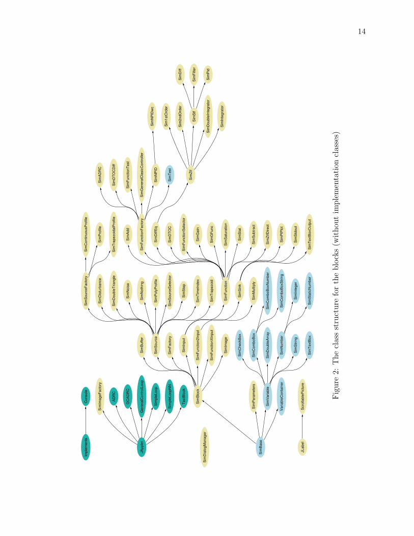
graphical manner. The following diagrams were generated by the java2dot program.3
From the graphical diagram shown in Figure 2 it can be seen that every SimBlock is
an extension of the three main building blocks. The class structure for the blocks is
graphed without the implementation classes. The entire hierarchal class structure is
displayed in Figure 3. Additional figures are displayed in Appendix D.
1http://academic.csuohio.edu2In the future multiple outputs could also be implemented to provide for state space representa-
tion of systems.3see Appendix A.3 for information about the java2dot program
14
JLab
elS
crol
labl
ePic
ture
Sim
Ztf
Sim
1stO
rder
Sim
2ndO
rder
Sim
Stf
Sim
Dou
bleI
nteg
rato
r
Sim
Inte
grat
orS
imFu
nctio
n
Sim
Add
Sim
Func
tionF
acto
ry
Sim
Diff
Eq
Sim
DTO
C
Sim
Func
tionS
elec
tor
Sim
Gai
n
Sim
GFu
nc
Sim
Sat
urat
ion
Sim
Sta
t
Sim
Sub
tract
Sim
ZtfD
irect
Sim
AD
RC
Sim
DTO
CD
iff
Sim
Func
tionT
est
Sim
Gen
eral
Cla
sicC
ontro
ller
Sim
NP
ID
Sim
Test
Sim
Bas
e
Sim
Blo
ck
Sim
Par
amet
ers
Sim
Var
iabl
e
Var
iabl
eCon
tain
er
Sim
Buf
fer
Sim
Sou
rce
Sim
Fact
ory
Sim
Inpu
t
Sim
Func
tion2
Inpu
t
Sim
Func
tionX
Inpu
t
Sim
Imag
e
Sim
Sou
rceF
acto
ryS
imC
ontin
uous
Pro
file
Sim
Pro
file
Sim
Trap
ezoi
dalP
rofil
e
Sim
Dia
logM
anag
er
Sim
Diff
Sim
Filte
r
Sim
Pid
Sim
Dis
turb
ance
Sim
Dou
bleT
riang
le
Sim
Noi
se
Sim
Not
hing
Sim
Pol
yPro
file
Sim
Sou
rceS
elec
tor
Sim
Ste
p
Sim
Tim
eInd
ex
Sim
Trap
ezoi
d
Sim
Sin
k
Sim
Mul
tiply
JApp
let
Sim
Imag
eFac
tory
AD
RC
GC
AD
RC
Gen
eral
Con
trolL
oop
Sim
pleL
oop
Sim
pleL
oopN
N
Test
Blo
ck
Sim
NP
IDw
c
Sim
PtP
lot
Sim
Std
out
Sim
Text
Box
Out
put
Sim
Che
ckB
ox
Sim
Com
boB
ox
Sim
Dou
bleA
rray
Sim
Num
ber
Sim
Stri
ng
Sim
Text
Box
Sim
Com
boB
oxN
umbe
r
Sim
Com
boB
oxS
tring
Sim
Inte
ger
Sim
Sta
ticN
umbe
r
impl
emen
tsC
onso
le
Fig
ure
2:T
he
clas
sst
ruct
ure
for
the
blo
cks
(withou
tim
ple
men
tation
clas
ses)

15
Scrollable
ScrollablePicture
JLabel
SimPanelable
Sim1stOrder
Sim2ndOrder
SimADRC
SimFunctionFactory
SimContinuousProfile
SimSourceFactory
SimDiff
SimStf
SimDiffEq
SimDisturbance
SimDoubleTriangle
SimDTOC
SimDTOCDiff
SimFactory
SimFilter
SimFunctionSelector
SimFunctionTest
SimGain
SimGeneralClasicController
SimGFunc
SimImage
SimNoise
SimNothing
SimNPID
SimParameters
SimPid
SimPolyProfile
SimProfile
SimPtPlot
SimSaturation
SimSourceSelector
SimStat
SimStep
SimTest
SimTextBoxOutput
SimTimeIndex
SimTrapezoid
SimTrapezoidalProfile
SimVariable
VariableContainer
SimZtfSimDoubleIntegrator
SimIntegrator
SimFunction
SimAdd
SimSubtract
SimZtfDirect
SimBase
SimBlock
SimBuffer
SimSource
SimInput
SimFunction2Input
SimFunctionXInput
SimDialogManager
Iterator
Simulatable
ADRC
Console
GCADRC
GeneralControlLoop
SimpleLoop
SimpleLoopNN
TestBlock
HasOutput
SimSink
SimMultiply
JApplet
SimImageFactory
HasInput
SimNPIDwc
SimStdout
SimCheckBox
SimComboBox
SimDoubleArray
SimNumber
SimString
SimTextBox
SimComboBoxNumber
SimComboBoxString
SimInteger
SimStaticNumber
implements
Figure 3: The entire hierarchal class structure of the project

16
2.2.2 Class Inheritance Structure
An interesting example explanation of the hierarchal path is the following:
SimPid → SimStf → SimZtf
→ SimDiffEq → SimFunction
→ SimBlock → SimBase (2.1)
This means that SimPid is a SimStf, and a SimStf is a SimZtf and so on. Each
implementation has all of the features of the inherited classes. The sorted ascending
list of increasing levels of abstraction and what feature each inherited block provides
is shown in Table I.
Table I: Example hierarchy path of a PID controller
Class name provides
SimBase simple title and description structuresSimBlock the ability to interface with the rest of
the simulation librarySimFunction the functionality of inputs and outputsSimDiffEq the ability to create, display, and edit
discrete difference equationsSimZtf the ability to create, display, and edit
z transfer functions and convert themto discrete difference equations
SimStf the ability to create, display, and edits transfer functions and convert themto z transfer functions
SimPid the specific transfer function for pro-portional, integral and derivative con-trol
2.2.3 Block Interconnection
A key component of the structural implementation was the means of connecting
each of the desired blocks together. In order to reach the speed required for real

17
time dynamic response, practicality and efficiency were considered when designing
the interconnection buffers. Considering the fact that the amount of data history
required for any block is defined by the order of the difference equation, and that the
order is most often less than ten for most systems, the memory used for the history
can be kept minimal. The reduced size buffers are efficient because extra memory is
not required, and they are practical because the same implementation scheme can be
used in an embedded system.
The SimBuffer was created to store the recent history of each block. This
buffer was also used as the software implementation of a connection between blocks
to create the desired signal. The connections are made with a supervisory class called
SimFactory. More information on the implementation of the connection and flow of
data of the classes is in Chapter 3.
2.3 GUI Development
Once the functional structure was well-defined, simple GUI elements were
added to give a visual demonstration of the library.
The GUI was built with Java’s newer GUI Application Programmers Interface
(API) called Swing. Just as the object-oriented nature of the design appropriately
constructed the hierarchal nature of the library, it also matched the implementation of
the GUI. Each of the SimBlocks that are connected can generate their own adjustment
dialogs, as well as other windows like plots. A simple block would display its own
information while the detail of a more complex block is automatically generated from
the separate building components from which it is extended. An example of the simtk
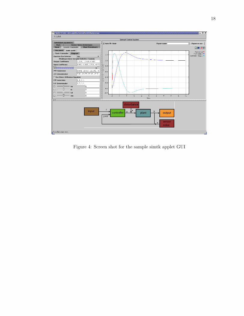
applet which incorporates many levels of the hierarchal GUI can be seen in Figure 4
and Figure 40. The use of this applet is more fully described in Appendix C.
18
Figure 4: Screen shot for the sample simtk applet GUI

CHAPTER III
DATA FLOW IMPLEMENTATION
The structural inheritance implementation of the relationship between blocks
can easily be seen and was described in the previous chapter. However, in order to
understand how the classes all work together, the interaction and data flow organi-
zation between the simtk library blocks needs to be described. Both developers (who
would add on to the library and use if for specific purposes) and users of a constructed
simulation package should understand the fundamental flow of the data. Developers
should build blocks consistent to the package as well as understand how a system is
designed.
19

20
3.1 Developer’s Viewpoint
In the same way that a person can drive a car without knowing exactly how
a gasoline engine works, it is not necessary for a user to understand the underlying
functions of the software library. However, a more in-depth knowledge is important
for a designer who would want to add or modify a car’s features and functionality.
In the same way, it is important for a software developer, to understand the under-
workings of the code to design and build additional features to the system.
3.1.1 Top-level Managing Class
A software developer would primarily be interested in how pieces of the system
are connected. The previous chapter described that there were many simulation
blocks created. There is a need for a top-level managing class that will control,
manage, and act as a base to connect each of the simulation pieces together. This
class is called the SimFactory, which is used as a means to store the global-type
variables, such as simulation parameters, for the final time and step size that are
used for every block. Furthermore, with the simulation information the factory class
knows how many iterations to perform on the blocks to reach the desired simulation
period. It performs the iterations of the blocks and interconnection buffers at the
appropriate times and steps through the system. Presently the order that the blocks
are added to the factory class is the same order that the blocks are iterated. There is
no algorithm for simulation order discovery.1 Therefore, some knowledge is needed to
correctly order and connect the blocks prior to simulation. This is especially true for
some controllers that need the plant information before the controller is calculated.
Presently, the top-level class is the sand-box where the library components are placed
1Simulation order discovery is a future area of research (see Section 8) to add to the simulationpackage which would be necessary for a graphical environment similar to Simulink.

21
and held together.
The overseeing class is also useful when built in a hierarchal manner. Designing
it to be included within itself allows an abstraction allowing complex simulation blocks
to appear as any other simple functions, only with more internal functionality. The
SimFunctionFactory class is an example of a SimBlock that externally looks like an
ordinary SimFunction. However, internally the complexity can be built by combining
other blocks. For the hierarchy abstraction, the SimFactory is wrapped, for example,
by an applet that implements the HasFactory interface. One such applet is the
GeneralControlLoop.java applet, listed in Appendix E on page 103, which contains a
SimFactory and shows the basic requirements to set, configure, and make use of the
library.
It is also helpful to see a containment graph of classes to get a feel of the
relation and use between various classes. The following diagram was generated by
the containment.pl program.2 It simply illustrates how the SimFactory makes use of
the other blocks and also requires a few of the global parameters which it passes to
the rest of the simulation. A simplified example, of the containment of classes for the
GeneralControlLoop applet, with some classes removed, is illustrated in Figure 5.
2see Appendix A.3 on page 89 for information about the containment.pl program which uses thegraphviz dot language format to generate directed graphs

22
GeneralControlLoop
SimParameters
SimFactory
SimTextBoxOutput
SimPtPlot
SimImage
SimSubtract
SimFunctionSelector
SimStep
SimSourceSelector
SimGain
SimADRC
SimAdd
SimGeneralClasicController
SimProfile
SimSource
SimFunction
SimSink
SimBlock
Simulatable
SimBuffer
SimPanelable
Simulation
SimTabBox
SimDiffEq
SimFucntionSelector
SimComboBoxString
SimNumber
Simple
SimFunctionFactory
Figure 5: Simplified example containment of classes for the GeneralControlLoop ap-
plet

23
3.1.2 Setting Up a Simulation
There are only a few major steps to setup a desired simulation. The three
major sections are loading, connecting and simulating. The first step in setting up a
system is to define what is needed. Classes from the simtk library can be instantiated
statically by code or dynamically by using one of the SimSelectors to load a desired
function at runtime. After the blocks are loaded into memory, they need to be added
to the simulation factory to be simulated. While adding the blocks to the factory the
blocks can also be connected. The SimFactory.add() function also takes the block
that should be connected to the input of the block currently being added.3 Finally,
when all the required blocks are connected, the SimFactory.doSimulation() can be
called. See Listing E.1 on page 117 for a single example of using and creating a
control system with the library.
3.1.3 Building Blocks
There are also three major steps in creating or building more functions to
the library: extend a block, add the adjustable variables, and override the iteration
definition.
First of all, the choice of a block needs to be made that already has the functions
that implements similar operations and the new functionality can simply be added.
Most extended blocks are built from SimSource, SimSink, SimFunction or a derivative
of these such as or SimZtf, SimStf.
Once the parent class is selected, the new functionality is added by selecting
the types of variables4 that are needed from the simtk.variables package. These are
3As an example the add function could be: add([the block to be added],[title of the block], [outputof the block to connect to this one])
4Within these variables the GUI is developed, each block knows its own variables and each variableknows how to display its own GUI a few of the variables are strings(TextFields), doubles(Sliders andtextFields), double arrays(comma separated text lists), and boolean (checkbox).

24
then added to the VariableContainer where the other variables are also stored.
The final step to define a block and where the actual functionality is stored
is within the iteration definition. The function doIteration() is called whenever a
parameter is updated. For example, if a variable is changed with the slider this
function will make the appropriate changes. This is where the code to calculate the
new outputs or parameters from the current inputs or variables is calculated. For
some classes such as SimStf, the doIteration() is constant but the parameters are
redefined. In this case simply overriding the reDefine() function will load the desired
transfer function at a parameter update. See Listing E.2 on page 119 for a single
example of extending an S transfer function into a general second order plant.
The developer interested in modifying the code and adding to the library should
first understand the bases and underlying theory of the package from the information
in these and the following chapters. For reference of the code structure and how to
use the library, the example code for the applets can be followed. The main source
and documentation of the API is contained in the javadoc-generated documentation
for the project.
3.2 User’s Viewpoint
While the knowledge of the underlying structure is not required for the user
it is still necessary to understand how the system is held together. There are a few
main ideas that the user should grasp.
First of all, it is imperative that the nature of the system is understood. The
results of the simulation are meaningless unless the user understands what they are
simulating. Although this may sound trivial, it is important to achieve appropriate
results. A user must enter meaningful inputs to achieve meaningful outputs.
A second, corresponding, comprehension required from the user is that the

25
simulation accuracy is dependent upon the specified step size. To make the real time
effect transparent the simulation size is kept small. However, the step size for the
simulation may need to be reduced by the user to achieve more accurate results.
Finally, along with the step size, there are a few global parameters that make
adjustments across the whole simulation. A few of the current global parameters are
the final simulation time and the step size. The step size is an important criteria for
some discrete controllers5, which require a knowledge of the step size for calculation
of the control signal.
While these fundamental ideas hold to the general nature of the simtk library,
additional information should be given by the developer to the user for specific fea-
tures. As an example, a small user’s guide of the present demonstration applet is
provided in Appendix C on page 103.
5One example is the Discrete Time Optimal Control. See Chapter 5 for more information.
PART II
SYSTEM FUNCTIONALITIES
AND APPLICATION
26

CHAPTER IV
DIFFERENTIAL EQUATION SOLVER
This chapter and the following chapters will go further into the depths of
the core mathematics for the simulation package. The most important mathematical
function for a simulation package is how the system is expressed, modeled and solved.
Matlab contains a broad selection of differential equation solvers, but without the
help of Simulink, constructing nonlinear systems is difficult. SysQuake provides an
ode451 solver, but expressing a system in this form restricts the model to time domain
differential equations. Although this may be convenient for the solver, it is not for
the user. Often it is helpful to express systems in terms of other variables such as
frequency or even more abstract references to help model nonlinear systems. For the
speed requirements of the real time simulation and tuning, basic difference equations
for discrete time solutions have been chosen as the basic simulation functions while
further functionality is overlaid.
A comparison is made, in Section 4.1, between several differential equation
methods and the reasons that the Tustin method was chosen over the Simple Euler
14th Runge Kutta algorithm
27

28
method is given. Using the Tustin method, algorithms are developed in Section 4.2
to convert various system expressions into a difference equations.
4.1 Comparison of Ode Solvers
There are several types of methods for computerized differential equation so-
lutions. Simple Euler and Tustin are the two major methods which receive the most
attention when being compared for this project. The Simple Euler is one of the sim-
plest and most often used in implementation of embedded systems while Tustin is
slightly more involved.
The ordinary differential equation solver algorithms can become confusing since
there are many names for the same algorithm. Different fields have different names.
The primary solver that is used in the simtk library is called Tustin by the control
theorists, Trapezoidal by Mathematicians, and Bilinear by computers scientists. Since
this research centers around control theory, Tustin will be used to denote this type of
solver.
4.1.1 Simple Example Problem for Comparisons
A simple definition of a differential equation of a system is defined in (4.1).
Various solvers are then applied to the same function and compared to each other
and the exact solution.
y′(t) = f(t, y(t)) (4.1)
y(t0) = y0 (4.2)
The following comparisons plots were generated from a Java applet at the University
of British Columbia to compare various differential equation solvers for the same

29
function.2
Figure 6: Comparison of ode solvers with 5 iterations
Figure 7: Comparison of ode solvers with 10 iterations
Figure 6 and Figure 7 demonstrate that the Tustin algorithm has a more
accurate solution to the actual solution than the Simple Euler method, however with
only these graphs it is difficult to get a picture of how much better it behaves.
The following two graphs give an understanding of the benefits of using the
slightly more advanced algorithm3.
2This Applet can be found at: http://www.math.ubc.ca/~feldman/demos/demo2.html3The level of sophistication of the Tustin and Euler algorithms are derived in Chapter 4.2.

30
Figure 8: Comparison of ode solvers with 20 iterations
Figure 9: Comparison of ode solvers with 200 iterations
By increasing the number of iterations to 20, as shown in Figure 8, the Tustin
algorithm is shown to reach quite close, at least at this scale, to the exact solution. In
order to reach this same level of accuracy with the Simple Euler method the number
of iterations is increased to 200 in Figure 9. Almost 10 times the samples needed for
the Tustin solver which is only sightly more involved. This reduction in the need of
sampling time is directly related to the real world problem of sampling time and the
cost of faster analog to digital converters.
The final comparison in Figure 10 shows the advantage of the Runge-Kutta
algorithm.

31
Figure 10: Comparison of ode solvers with 3 iterations and Runge-Kutta
Although it is significantly better than the Simple Euler and even the Tustin,
especially for smaller sampling times, for now4, the complexity of the implementation
of the algorithm is not worth the accuracy gained over the simplicity of the Tustin
algorithm at higher sampling rates. The Runge-Kutta algorithm is significantly more
involved and not suited for the application of real time control especially for expor-
tation of algorithms to embedded systems.
The Tustin algorithm is significantly more accurate than the Simple Euler
method with only a slightly more involved implementation. The primary benefit
is an almost ten-fold decrease in the sample rate or step-size for the same level of
accuracy, which is the reason it was chosen as the primary solution for the engine of
this project.
4.2 Differential Equation Solver Engine
The core of the simulation package is the differential equation solver engine. It
is important to understand its purpose and specifically describe the implementation.
At first, many specific discrete equation solutions were derived from commonly used
4In the future it would be an interesting area of research to test algorithms at extremely lowsampling rates and incorporate the Runge-Kutta solver

32
continuous functions. For an extensible library, multiple levels of the solver needed to
be designed separately in a modular form. Instead of a static specific transformation,
a fundamental general s to z transform algorithm was then designed around the
Tustin method. This was converted directly to the discrete difference equation with a
general conversion from z transform functions. These various levels of conversions are
overlaid transparently and executed in succession to produce the illusion of various
types of model descriptions in a single simulation environment.
4.2.1 Specific Conversions from Continuous Form to Discrete
The following sections derive the discrete solutions as z transform functions,
for specific blocks such as integrators, second and first order responses, and PID. The
derivation is shown for the Simple Euler and the Tustin method to show the differ-
ence in implementation complexity. All of the difference equations were ultimately
solved using Tustin’s method, which is simple but still has a significant performance
enhancement over the simple Euler method.5
Simple Euler
The Simple Euler method used for the conversions of the s to z domain is
defined by substituting s with the following equality. Where s is the Laplace transform
of a pure differentiator,
s =−1 + z
T(4.3)
The simple integrator becomes
1
s→ T
−1 + z(4.4)
5the performance enhancement can be shown with the Java applet comparing the Simple Euler,trapezoidal and Runge-Kutta methods in Section 4.1

33
A double integrator after some reduction then becomes
1
s2→ T 2
1− 2z + z2(4.5)
These simple equations demonstrate that the Simple Euler method is quite simple to
implement, however it does not provide a very efficient or accurate conversion when
compared with some other methods as described in Section 4.1.
Tustin
The Tustin method proves to be far more accurate and efficient than the Sim-
ple Euler but only slightly more involved when doing the conversions of the s to z
domain [1]. This method is defined by substituting s in a Laplace transform with the
following equality.
s =2 (−1 + z)
T (1 + z)(4.6)
The simple integrator then becomes
1
s→ T + T z
−2 + 2 z(4.7)
A double integrator after some reduction then becomes
1
s2→ T 2 + 2 T 2 z + T 2 z2
4− 8 z + 4 z2(4.8)
A first order plant, where a is the pole location becomes
1
s + a→ T + T z
−2 + a T + 2 z + a T z(4.9)
A second order plant, where ω is the frequency and ζ is the damping ratio is given as

34
ω2
s2 + 2ζω + ω2→
T 2 ω2 + 2 T 2 z ω2 + T 2 z2 ω2
4− 4 T ζ ω + T 2 ω2 + 2 z (−4 + T 2 ω2) + z2 (4 + 4 T ζ ω + T 2 ω2)(4.10)
A second order plant where ω = ζ = 1 is shown to be slightly simpler
1
s2 + 2 + ω2→ T 2 + 2 T 2 z + T 2 z2
4− 4 T + T 2 − 8 z + 2 T 2 z + 4 z2 + 4 T z2 + T 2 z2(4.11)
A PID controller where the proportional, integral, and derivative gain are defined as
kp, ki, and kd respectively is derived as
kps + kds2 + ki
s→
4 kd − 2 kp T + ki T2 − 8 kd z + 2 ki T
2 z + 4 kd z2 + 2 kp T z2 + ki T2 z2
−2 T + 2 T z2(4.12)
A pure differentiator can not be implemented since it results in an improper transfer
function, but approximate results can be obtained. The second order approximate
differentiator has been proven to give excellent differentiation, in [12], with relatively
simple implementation. The derived z transform function is given as
s
(τs + 1)2→
−2 T + 2 T z2
T 2 + 2 T 2 z + T 2 z2 − 4 T τ + 4 T z2 τ + 4 τ 2 − 8 z τ 2 + 4 z2 τ 2(4.13)
General Transfer Function Derivations
The specific solutions show relatively simple difference equations to implement
such functions as second-order plants and PID controllers. A rather flat solution for
a simulation package could simply have a large library of these solutions for every

35
desired model. However, to create an extensible, powerful, dynamic package rather
than a limited set of static predefined blocks, general describing solutions are solved.
The first five orders of a Laplace polynomial are shown below.
The general 0th order polynomial
Gp = n0 (4.14)
transforms to
n0. (4.15)
The general 1st order
Gp = n1s + n0 (4.16)
transforms to
−2 n1 + n0 T + 2 n1 z + n0 T z. (4.17)
The general 2nd order
Gp = n2s2 + n1s + n0 (4.18)
transforms to
4 n2 − 2 n1 T + n0 T 2 − 8 n2 z
+2 n0 T 2 z + 4 n2 z2 + 2 n1 T z2 + n0 T 2 z2. (4.19)
The general 3rd order
Gp = n3s3 + n2s
2 + n1s + n0 (4.20)

36
transforms to
−8 n3 + 4 n2 T − 2 n1 T 2 + n0 T 3
+24 n3 z − 4 n2 T z − 2 n1 T 2 z + 3 n0 T 3 z
−24 n3 z2 − 4 n2 T z2 + 2 n1 T 2 z2 + 3 n0 T 3 z2 + 8 n3 z3
+4 n2 T z3 + 2 n1 T 2 z3 + n0 T 3 z3. (4.21)
The general 4th order
Gp = n4s4 + n3s
3 + n2s2 + n1s + n0 (4.22)
transforms to
16 n4 − 8 n3 T + 4 n2 T 2 − 2 n1 T 3 + n0 T 4 − 64 n4 z + 16 n3 T z
−4 n1 T 3 z + 4 n0 T 4 z + 96 n4 z2 − 8 n2 T 2 z2 + 6 n0 T 4 z2 − 64 n4 z3
−16 n3 T z3 + 4 n1 T 3 z3 + 4 n0 T 4 z3 + 16 n4 z4
+8 n3 T z4 + 4 n2 T 2 z4 + 2 n1 T 3 z4 + n0 T 4 z4. (4.23)
4.2.2 General s to z Transform Matrices
The previous results can be displayed in a more concise manner in the form of
matrices. This is very important for the simplicity of the implementation in software
for the solver engine. A general s to z (s2z) transform matrix can be derived as
follows:
Zn = Mn · Sn ·Tn (4.24)

37
where n is the order of the system and, sn is the coefficient of s with the exponent
of n.
Sn =
s0
s1
s2
...
sn
(4.25)
and
Tn =
T 0
T 1
T 2
...
T n
(4.26)
With the above definitions of Mn, the general-ordered Laplace polynomials are sum-
marized in the following matrices.
M0 =
(1
)(4.27)
M1 =
−2 1
2 1
(4.28)
M2 =
−4 −2 1
−8 0 2
4 2 1
(4.29)
38
M3 =
−8 4 −2 1
24 −4 −2 3
−24 −4 2 3
8 4 2 1
(4.30)
M4 =
−16 −8 4 −2 1
−64 16 0 −4 4
−96 0 −8 0 6
−64 −16 0 4 4
16 8 4 2 1
(4.31)
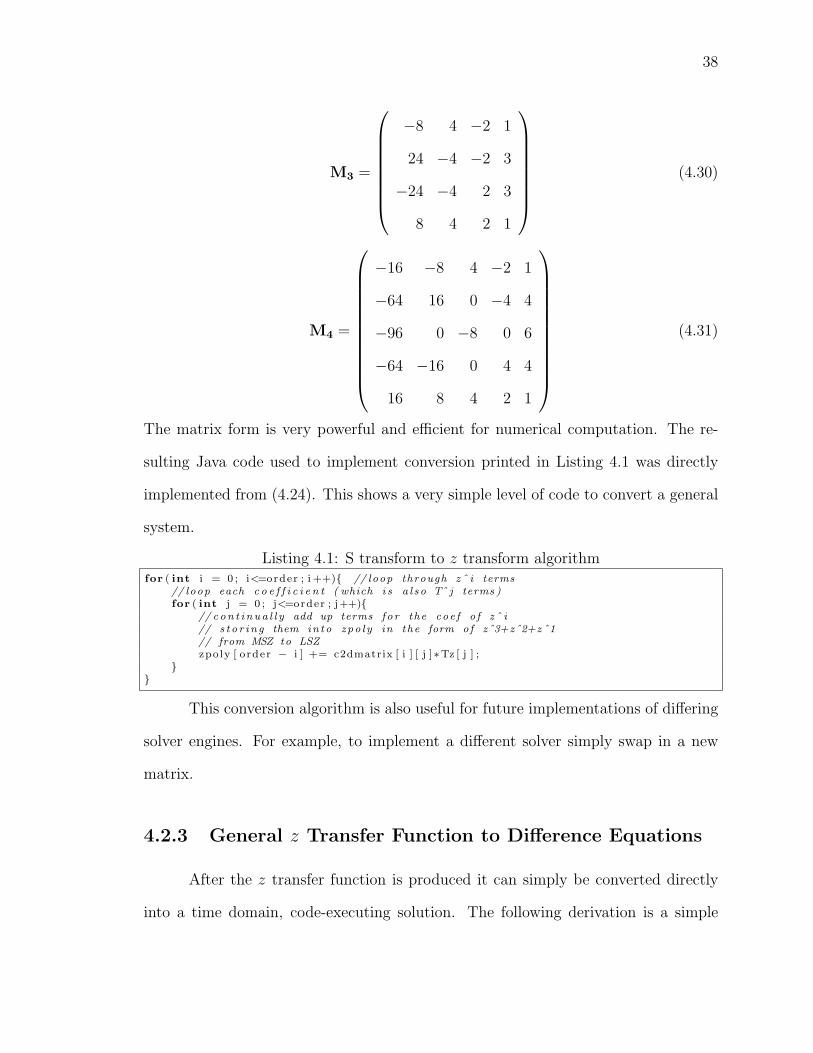
The matrix form is very powerful and efficient for numerical computation. The re-
sulting Java code used to implement conversion printed in Listing 4.1 was directly
implemented from (4.24). This shows a very simple level of code to convert a general
system.
Listing 4.1: S transform to z transform algorithmfor ( int i = 0 ; i<=order ; i ++){ // loop through zˆ i terms
// loop each c o e f f i c i e n t ( which i s a l s o Tˆ j terms )for ( int j = 0 ; j<=order ; j++){
// con t i nua l l y add up terms fo r the coe f o f zˆ i// s t o r i n g them in to zpo l y in the form of zˆ3+zˆ2+zˆ1// from MSZ to LSZzpo ly [ order − i ] += c2dmatrix [ i ] [ j ]∗Tz [ j ] ;
}}
This conversion algorithm is also useful for future implementations of differing
solver engines. For example, to implement a different solver simply swap in a new
matrix.
4.2.3 General z Transfer Function to Difference Equations
After the z transfer function is produced it can simply be converted directly
into a time domain, code-executing solution. The following derivation is a simple

39
algorithm for automatically converting a general z transfer function into its specific
difference equation for simulation or code generation.
Using the general 4th order transfer function a general z transfer function to
discrete (z2d) form equation can be derived6 with input r and output y defined as:
y
r=
n0z4 + n1z
3 + n2z2 + n3z
1 + n4z0
d0z4 + d1z3 + d2z2 + d3z1 + d4z0(4.32)
The form of this equation can be converted to negative powers of z by multiplying
by:
z−4
z−4(4.33)
Then we can solve for the output, y
y =1
d0
((n0r + n1rz−1 + n2rz
−2 + n3z−3 + n4z
−4)
−(d1rz−1 + d2rz
−2 + d3z−3 + d4z
−4)) (4.34)
By inspection we can see that we could further reduce this formula to an even more
general form of the output for a q ordered system.
y =
∑qi=1(nirz
−i − dirz−i) + n0r
d0
(4.35)
By the inverse z transform we know that
z−i → y(k − i) (4.36)
Once in this form, we can easily read off the difference equation. The entire process
can now easily be implemented in code with an iterative loop for any ordered system.
6solved 4/26/02

40
This derived formula can be implemented in Java code, which is listed in
Listing 4.2.7
Listing 4.2: z transform to difference equation algorithmdouble tempsumterms = 0 ;
for ( int i =1; i<=zorder ; i++){tempsumterms += num[ i ]∗ in . va l [ i ] − den [ i ]∗ out . va l [ i ] ;} ;
out . va l [ 0 ] = ( tempsumterms + num[ 0 ] ∗ in . va l [ 0 ] ) / den [ 0 ] ;
7this code is found in the SimZtf class within the doIteration function
CHAPTER V
CONTROLLER DESIGN AND
IMPLEMENTATION
With the core of the solver implemented in Section 4.2, control modules can
now be built. There are a number of important control theory algorithms and methods
such as parameterization in [8], Nonlinear-proportional-integral-derivative (NPID)
in [13], Active Disturbance Rejection Control (ADRC) in [11], and Discrete Time
Optimal Control (DTOC) [10], that are essential to this project’s purpose of simplis-
tic, practical tuning which are implemented in this project and discussed within this
section. Many control systems are simple filters and Section 5.6 is devoted to them
as well as the important use of pre-filters in control designs.
41

42
5.1 Parameterization
Parameterization is a control methodology introduced, in [8], for vastly im-
proving the tuning of a system. It allows for the fundamental understanding of a
system and relates many defining parameters into one super-parameter which has a
direct correspondence to the system, usually in terms of the speed or bandwidth of
the system.
For example, the parameters of a PD controller can be optimally derived for
a double integrator plant, 1s2 . The closed loop form is put into a critically damped
response with a bandwidth of ωc. To get this type of response kd and kp are solved
as:
kd = 2ωc (5.1)
kp = ω2c (5.2)
Parameterization is used to vastly simplify the advanced controllers, such as ADRC.
This, as well as some more familiar controllers are described in the following sections.
5.2 Approximate PID
The proportional-integral-derivative (PID) controller, in [2], is a prevalent con-
troller due to its effectiveness and simplicity. With the inclusion of parameterization,
it becomes an even more efficient controller since it can easily be tuned for optimal-
ity for a desired bandwidth, instead of using the tedious trial-and-error tuning. The
definition of the PID equation can be written as a function of the input error, e, and

43
the output from the PID, u.1
u = kpe + ki
∫e + kde (5.3)
Differentiating both sides of this equations yields
u = kpe + kie + kde (5.4)
Using the inverse Laplace transform and solving for u/e gives the transfer function
of the PID formula
u(s)
e(s)= kp +
ki
s+ kds (5.5)
Since this differentiator, s, is inexpressible in a real system, an approximate differen-
tiator is required. An appropriate, sufficient, approximate differentiator, as explained
in [12], equation can be expressed in the s domain as:
s =s
(τs + 1)2(5.6)
Figure 11 demonstrates an example 2nd order approximate derivative on a step func-
tion to demonstrate the effect of tau=1,0.5,0.25.
1derived on 4/27/02

44
0.0
0.2
0.4
0.6
0.8
1.0
1.2
1.4
0 1 2 3 4 5 6 7 8 9 10time
magnitude
step
tau = 1
tau = 0.25
tau = 5
Figure 11: 2nd order approximate derivative with tau=1,0.5,0.25 on a step function
Within the PID equation, s can be substituted with the equation above to get
the approximate PID transfer function
u(s)
e(s)= kp +
ki
s+ kd
s
(τs + 1)2(5.7)
(5.7) can be algebraically solved as a transfer function:
u(s)
e(s)=
s3(kpτ2) + s2(kd + 2kpτ + kiτ
2) + s(kp + 2kiτ) + ki
s3(τ 2) + s2(2τ) + s(1) + s(0)(5.8)
This simple but powerful and popular controller in this form is ready for realizable
implementation.
5.3 Nonlinear PID
Nonlinear PID, from [13], is an extension of the standard PID discussed in the
previous section, which simply defines a nonlinear gain-scheduled region in terms of
error for the P, I, and D parameters. Each term has carefully designed constraints
that define the specific gain values for regions of low and high error. For example,
the primary function of the nonlinear region is to have a high gain when the error

45
is small and small gain when the error is large, rather than a continuous gain for all
error levels.
The nonlinear PID control law can be described as
u = Gkp(e)e + Gki(e)
∫e + Gkd
(e)e (5.9)
where Gx(e) is a specifically designed regional gain for x and is a function of the
error.
One simple function that implements these regions of low and high gain for
varying errors is called the GFunction, which is a simple implementation using 4
regions of constant gains. It is the basis of the nonlinear PID used within the ’simtk’
library. The definition of the G function is described in (5.10).
Gx(e, kp1, kp2, kn1, kn2, wp, wn) =
e > 0
e · kp1 |e| < wp
e · kp2 |e| ≥ wp
e ≤ 0
e · kn1 |e| < np
e · kn2 |e| ≥ np
(5.10)
where
e is the error,
kp1 is the positive small error gain constant,
kp2 is the positive large error gain constant,
kn1 is the negative small error gain constant,
kn2 is the negative large error gain constant,
wp is the positive width of low error region,
And wn is the negative width of low error region.
This can be directly implemented in the following Java code example.
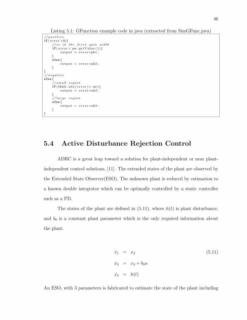
46
Listing 5.1: GFunction example code in java (extracted from SimGFunc.java)// p o s i t i v ei f ( e r ro r >0){
// i s in the f i r s t gain widthi f ( e r ro r < pw. getValue ( ) ){
output = e r r o r ∗pk1 ;}else {
output = e r r o r ∗pk2 ;}
}// nega t i v eelse {
// smal l reg ioni f (Math . abs ( e r r o r )< nw){
output = e r r o r ∗nk2 ;}// l a r g e reg ionelse {
output = e r r o r ∗nk2 ;}
}
5.4 Active Disturbance Rejection Control
ADRC is a great leap toward a solution for plant-independent or near plant-
independent control solutions, [11]. The extended states of the plant are observed by
the Extended State Observer(ESO). The unknown plant is reduced by estimation to
a known double integrator which can be optimally controlled by a static controller
such as a PD.
The states of the plant are defined in (5.11), where h(t) is plant disturbance,
and b0 is a constant plant parameter which is the only required information about
the plant.
x1 = x2 (5.11)
x2 = x3 + b0u
x3 = h(t)
An ESO, with 3 parameters is fabricated to estimate the state of the plant including

47
the disturbance:
z1 = z2 + B1(y − z1) (5.12)
z2 = z3 + B2(y − z1) + b0u
z3 = B3(y − z1)
The ADRC control law is then shown as
u =u0 − z3
b0
(5.13)
A controller has now been built that is defined by 3 terms: B0,B1 and B3 plus b0. By
parameterization2, these terms can be derived in terms of controller bandwidth, ωc,
and observer bandwidth, ωo. These can then be solved3 for the linear ADRC for any
second order plant as two transfer functions shown in (5.14) and (5.15).
The block diagram in Figure 12 shows how the ADRC controller can be broken
into two sections for simple implementation.
r r
y+n
u
ADRC general controller
pre-filter (includes controller and observer)
feedback-filter (includes controller and observer)
Figure 12: ADRC block diagram controller depicting the separation into two transfer
functions
2See Section 5.1 for information on this control tuning method.3Rob Miklosovic solved this equation in the dual transfer function form in 04/02.
48
The feed-forward controller or pre-filter is defined as:
U(s)
R(s)=
ω2c [1 3ωo 3ω2
o ω3o ] · S
b0 [(1) (3ωo + 2ωc) (3ωo2ωc + ω2c + 3ω2
o) (0)] · S(5.14)
The feedback controller or feedback filter is defined as:
Y (s)
R(s)=
ω2c [(3ωoω
2c + 3ω2
o2ωc + ω3o) (3ω2
oω2c + ω3
o2ωc) (ω3oω
3c )] · S
b0 [(1) (3ωo + 2ωc) (3ωo2ωc + ω2c + 3ω2
o) (0)] · S(5.15)
where S is a column vector defined as:
S =
s3
s2
s1
s
(5.16)
A b0 guideline is proposed as:
b0 =Largest plant numerator coefficient
Highest order plant denominator coefficient(5.17)
Once this controller is in transfer function form it could easily be implemented in the
SimStf or SimZtf simulation blocks.4 The block diagram of this controller setup is
shown in Figure 25. The result is a controller that has very good disturbance rejection
and allowance for plant variability, and, more importantly, a simple way to tune with
a few reasonable parameters.
5.5 Discrete Time Optimal Control
The DTOC algorithm is another leap toward plant model independent control
design, discussed and derived in [10]. It is a controller formulated in a constructive
4see Chapter 4 on page 27

49
manner from the optimal control law. Its use in engineering, is very promising due to
the level of plant independence, the ease of tuning, and the beautiful implementation
simplicity of the algorithm.
DTOC is a discrete solution that comes from another controller called Con-
tinuous Time Optimal Control(CTOC) which has been around for some time. The
control law for this controller is shown in (5.18).
u = −rsign
(x1 +
x2|x2|2r
)(5.18)
This law is optimal but not practical due to the chattering that occurs near zero
error. The DTOC offers a solution and, not only provides a method to create a linear
region near zero error, but it reaches zero in optimal time. The DTOC control law,
shown in (5.19) along with the internal definitions, has a simple direct mapping to
an implementable algorithm.
u = fst(x1, x2, r, h) (5.19)
d = rh
d0 = hd
y = x1 + hx2
a0 =√
d2 + 8r|y|
a =
x2 + a0−d2
sign(y), |y| > d0
x2 + yh, |y| ≤ d0
fst = −
rsign(a), |a| > d
r ad, |a| ≤ d
where
u is the control signal,

50
x1 is e or the error signal,
x2 is e or the derivative of the error signal (which was obtained with a 2nd
order approximate derivative),
r is the saturation limit(maximum control output),
k is the step size scaling parameter to be raised in the presence of noise,
ts is the discrete sampling period,
h = kts is the DTOC step size.
The DTOC algorithm was implemented in code with a sample shown in the
following listing.
Listing 5.2: DTOC control algorithm implemented in java/∗∗DTOC, f s t func t i on .∗ from dr . Gao, 3/7/3∗ t h i s i s the magic s t u f f !∗/double f s t 2 (double x1 , double x2 , double u0 , double r , double h){
double d , d0 , y , a0 , a1 ;
d=r ∗h ;d0=d∗h ;y=x1−u0+h∗x2 ;a0=Math . s q r t (d∗d+8∗r ∗Math . abs (y ) ) ;i f ( y>d0 ) a1=x2+(a0−d ) /2 ;else i f ( y<−d0 ) a1=x2−(a0−d ) /2 ;else a1=x2+y/h ;
return(−r ∗usat ( a1 , d ) ) ;}
/∗∗ nonl inear uni ty sa tu ra t i on func t ion .∗ from dr . Gao, 3/7/3∗/double usat (double x , double de l t a ){
i f ( x>de l t a ) return ( 1 . 0 ) ;else i f ( x<−de l t a ) return ( −1 .0) ;else return ( x/ de l t a ) ;
}
The result is a controller that has very good disturbance rejection and extreme
plant variability with simple tuning and implementation.

51
5.6 Filters
Low-pass and high pass filters are an important building block and tool for
creating models of control systems. In the following sections, a few of the basic filters
are derived, and the important role of pre-filter use and design is discussed.
5.6.1 Pre-filters and Profiles
The use of pre-filters or profiles for the input control reference is an important
role of control system design that is often not emphasized enough. A step input is
often used as the only reference for simulation and design. This creates a host of
problems for design and real-world implementation. In the real world, an instanta-
neous jump from a signal level to another, is impossible. A step input creates the
largest error possible to the controller at a given instant. If, instead, the input is
slowly brought up to the desired value at a rate that the system can follow, it is much
easier for the controller since the error stays within a small region, and, therefore,
an overall better design. The control can also be made more active since overshoot
would be less likely.
In a motion application, it is physically evident why a profile is required. A step
input for position yields in an infinite velocity and acceleration which destroys motors.
Even a ramp input yields in an infinite acceleration. So, a method is required to slowly
bring up the reference and at the same time slowly bring up the first, second, and third
derivatives of the reference signal, for velocity, acceleration, and jerk, respectively.
The Trapezoidal Pre-filter
There are several methods to create a profile or pre-filter. One method is to
integrate a Trapezoidal input to get a slowly increasing curve, followed by a slowly
decreasing curve until the reference point is reached. In this way, a smooth response

52
for the velocity is assured. The equation defining a trapezoid is shown in (5.20).
y =
0 x < d
3gw
x− 3gdw
d < x < d + w3
< x < d
g d + w3
< x < d + 2w3
−3gw
x + 3gdw
+ 3g d + 2w3
< x < d + w
0 x > d + w
(5.20)
The various parameters in this equation are illustrated in Figure 13, and the response
is shown in Figure 14.
0.00.1
0.2
0.3
0.4
0.5
0.6
0.7
0.8
0.9
1.0
0 1 2 3 4 5 6 7 8 9 10time
magnitude
d
g
w
Figure 13: Trapezoidal source for profiles
0.00.1
0.2
0.3
0.4
0.5
0.6
0.7
0.8
0.9
1.0
0.0 0.5 1.0 1.5 2.0 2.5 3.0 3.5 4.0time
magnitude
trapezoid integrated trapezoid for profile
Figure 14: Profile generated from the integration of a trapezoidal input

53
The S-curve Pre-filter
Extending from the thought of the trapezoidal pre-filter, the S-curve is smooth
in not only the velocity but also in the acceleration. This causes it to be even on the
plant dynamics especially for application to motors. The S-curve can be generated
from an odd triangular form, which is shown in Figure 15, and defined by (5.21)
to (5.23).
-1.0-0.8
-0.6
-0.4
-0.2
-0.0
0.2
0.4
0.6
0.8
1.0
0 1 2 3 4 5 6 7 8 9 10time
magnitude
d
g
w/3 w/3 w/3
w
g
Figure 15: Triangular source for S-curve profiles
y = msmx + (−mmsxint) (5.21)
where
m =6g
w(5.22)

54
and
ms = 0; xint = 0 x < d
ms = 1; xint = d d < x < d + w6
ms = −1; xint = d + w3
d + w6
< x < d + w3
ms = 0; xint = 0 d + w3
< x < d + 2w3
ms = −1; xint = d + 2w3
d + 2w3
< x < d + 5w6
ms = 1; xint = d + w d + 5w6
< x < d + w
ms = 0; xint = 0 x > d + w
(5.23)
and the parameters, w as width, d as delay, and g as the gain, are illustrated in
Figure 15.
Critically Damped Functions
Another method to generate a curve that smoothly brings the value up to the
desired reference level is to simply use a general-second order transfer function after
a step input. This is a good solution because a transfer function can easily be put
into a difference equation, and the defining parameter for the pre-filter can easily be
adjusted with one meaningful bandwidth parameter, ωr. A general 2nd order profile
defined by ωr, is shown in (5.24) with the response shown in Figure 16.
R(s) =ω2
r
s2 + 2ωrs + ω2r
(5.24)

55
0.00.1
0.2
0.3
0.4
0.5
0.6
0.7
0.8
0.9
1.0
0.0 0.5 1.0 1.5 2.0 2.5 3.0 3.5 4.0time
magnitude
2nd order generated profile
step
Figure 16: Profile generated from a step and 2nd order input
Two pre-filters can be cascaded in a row, as in (5.25), to create an even
smoother profile on deeper levels.
R(s) =ω2
r
s2 + 2ωrs + ω2r
ω2r
s2 + 2ωrs + ω2r
(5.25)
This is a simple solution. However, for precise control it is ineffective since the
response never mathematically reaches the set point where the trapezoidal and the
triangular S curve are assured to reach the desired point in a desired time.
Polynomial Pre-filter
A final method to generate a pre-filter is via a derived polynomial which is
specifically designed so the first, second, third, and fourth derivatives are all still
continuous. This allows even higher orders of derivative continuity. Even the S-curve
presents some trouble at the triple derivative. The polynomial5, in (5.26), is simple to
implement and has a simple equation which produces great results. Tr is the desired
5This was extracted from a Matlab simulation that Rob Miklosovic had tested in 2/3.

56
rise time of the profile, and g is the gain or the final value of the profile.
y(x) = g
10x3
T 3r− 15x4
T 4r
+ 6x5
T 5r
x < Tr
1 x ≥ Tr
(5.26)
The plot where Tr is equal to five is shown in Figure 17.
0.00.1
0.2
0.3
0.4
0.5
0.6
0.7
0.8
0.9
1.0
0.0 0.5 1.0 1.5 2.0 2.5 3.0 3.5 4.0 4.5 5.0 5.5 6.0 6.5 7.0 7.5 8.0 8.5 9.0 9.5 10.0time
magnitude
polynomial profile
Figure 17: Profile generated from the simple polynomial with Tr = 5
5.6.2 General Normalized Butterworth Filters
Butterworth filters are the most basic filters for variety of needs such as low-
pass, high-pass and band-pass filters. Various orders of the Butterworth filters are
derived as follows.
The first order normalized butterworth filter6 is given as:
H(s) =1
s + 1(5.27)
The second order normalized butterworth filter is given as:
H(s) =1
s2 +√
2s + 1(5.28)
6The following normalized buterworth filters were found at: http://www.apicsllc.com/apics/Sr_3/Sr_3.htm

57
The third order normalized butterworth filter is given as:
H(s) =1
s3 + 2s2 + 2s + 1(5.29)
The fourth order normalized butterworth filter is given as:
H(s) =1(
s2 + 320
√26s + 1
) (s2 + 181
500
√26s + 1
) (5.30)
Low-pass, High-pass, Bandpass, and Bandstop Extension
The following equations demonstrate how to generate different filters from the
normalized butterworth filters. A helpful relationship for the conversion of radians to
Hertz is
ω = 2πf (5.31)
For the low-pass case:
s → s
ω(5.32)
For the high-pass case:
s → ω
s(5.33)
For the bandpass case:
s → s2 + ω2
Bs(5.34)
For the bandstop case:
s → Bs
s2 + ω2(5.35)

58
Lowpass
For the first order case, using (5.32), (5.27) is converted to the familiar transfer
function form:
H(s) =1
1ωs + 1
(5.36)
An example of the first order low-pass Butterworth filter filtering noise is shown in
Figure 18.
-1.0-0.8
-0.6
-0.4
-0.2
-0.0
0.2
0.4
0.6
0.8
1.0
0 1 2 3 4 5 6 7 8 9 10time
magnitude
noise
butterworth filter
Figure 18: 1st order low-pass Butterworth filter filtering noise
For the second order case, using (5.32), (5.28) is converted to the familiar
transfer function form:
H(s) =1
1ω2 s2 +
√2
ωs + 1
(5.37)
For the third order case, using (5.32), (5.29) is converted to the familiar transfer
function form:
H(s) =1
1ω3 s3 + 2
ω2 s2 + 2ωs + 1
(5.38)

59
Highpass
For the first order case, using (5.33), (5.27) is converted to:
H(s) =1
ωs
+ 1(5.39)
After some algebra the equation can be reduced to the familiar transfer function form:
H(s) =s
s + ω(5.40)
For the second order case, using (5.33), (5.28) is converted to:
H(s) =1
1s2 ω2 +
√2
sω + 1
(5.41)
After some algebra the equation can be reduced to the familiar transfer function form:
H(s) =s2
s2 +√
2ωs + ω2(5.42)
For the third order case, using (5.33), (5.29) is converted to:
H(s) =1
1s3 ω3 + 2
s2 ω2 + 2sω + 1
(5.43)
After some algebra the equation can be reduced to the familiar transfer function form:
H(s) =s3
s3 + 2ωs2 + 2ω2s + ω3(5.44)
From a few simple equations, a powerful library of control design tools has been built.
This included simple controllers to advanced controllers as well as the inclusion of
many types of filters.

CHAPTER VI
A GENERAL MODEL DIAGRAM
Chapter 5 described a number of control algorithms. In order to make a simple
tool to compare different controllers, a method for dynamically selecting and com-
paring a wide range of controllers is required.
The control system diagram is classically drawn and modeled after the dif-
ference in the error, while the pre-filters, feedback filter, and observers are modeled
separately. However, these and almost any controller1 can be combined for a more
general view and model of a controller which has two inputs and one output. Putting
any controller in this format allows the rest of the system being tested to remain the
same while various types of controllers in this general model structure can simply be
plugged in and fairly compared.
1for a single input single output system
60

61
6.1 Classic System
The control system traditionally has a structure with a loop formed around
a difference junction. This can be seen in Figure 19 and a more complex version
including the noise and disturbance modeling is shown in Figure 20.
controller plant outputinput
Figure 19: Simple classic controller without noise or disturbance
controller plant output
sensor noise
input
disturbance
r e
y+n
u y
Figure 20: Classic controller model setup with noise and disturbance
From these basic feedback structures, the system is expanded by slowly adding
more components to the appropriate positions. This is often required for a better
representation of the plant, but often the controller also requires additional informa-
tion and blocks in various places in the diagram. Once the complexity has begun to
build, it becomes increasingly difficult to fairly compare differing controllers.

62
6.2 Combined General System
Although the classical representation is a good model of many systems, an even
more general representation can be formed in terms of the controller within which
any control can be composed. For the sake of generality and pluggable architecture,
a more general feedback system could be written by block diagram reduction. The
summing junction for the error and reference can be internal to the controller so any
pre-filters or feedback filters can be realized. The new representation is shown in
Figure 21. This can be compared to the model in Figure 20 to see that the summing
junction is now just internal to the controller.
plantr
y+n
u ycontroller output
sensor noise
input
disturbance
Figure 21: New General controller model setup
This allows the same plant, sensor, disturbance and input structure to be
compared with any controller for a fair comparison and no redesign.
6.3 General Blocks
The general controller block itself with two inputs and two outputs as a general
form is illustrated in Figure 22.

63
r
y+n
ugeneral controller 2 inputs one output
Figure 22: New General controller block
An improved general controller block to include a pre-filter and feedback-filter
is shown in Figure 23.
r
y+n
u
improved general controller
pre-filter
feedback-filter
e classic controller ( ex. PID )
Figure 23: Improved General controller to include pre-filter and observer before sum-
ming loop
The entire system is the control design, and if a general controller is desired
the entire sum is a better description. By this method, controllers that do not use
error as an input can also be used. In general control diagram structure, the most
basic information is provided to the controller, which is the reference and the output.
If an error control is desired it can be internally calculated by a subtraction. Using
this description, more information than just the error is sent to the box creating a
more general controller block that any control design can be implemented within.
An example of the general controller block implementing a PID controller is

64
shown in Figure 24. If this general form PID block from Figure 24 is substituted into
the general controller system in Figure 21, the same classical control system that is
illustrated in Figure 20 is achieved by block reduction.
r e
y+n
u
general controller example
classic controller ( ex. PID )
Figure 24: New General controller block example using PID
An example of a general controller block using a ADRC is also shown in Fig-
ure 25.
r r
y+n
u
ADRC general controller
pre-filter (includes controller and observer)
feedback-filter (includes controller and observer)
Figure 25: ADRC Controller (which is a special case of the improved general controller
where error controller is unity)
A general control block is an important aspect when looking towards a simple
system for users to model systems and compare various controllers. It would also

65
play an important role in computer-automated control design for testing of various
controllers.
CHAPTER VII
ACTIVE OPTIMIZATION CONTROL
Parameterization, as discussed in Chapter 5, allows the many variables of a
system to be reduced to one conclusive parameter that has a physical meaning to
the system, such as the bandwidth. This idea of parameterization offers a whole
new approach to active tuning. Instead of auto-tuning in terms of extracting plant
information for new control values, the single parameter can be actively optimized to
a threshold or limit inherent to the system. The design can then be automated by
a computer as long as the requirements are appropriately defined and the method to
quantify these requirements is established. Although this scheme of optimization is
not directly implemented in the simtk library, the functionality and functions have
been built in place for its future development and discussed in Chapter 8.
7.1 Threshold Limit Requirement
Understandably, different systems require different constraints. Some are more
dependent on the level of the control signal noise that occurs before the system
66

67
goes unstable, which is ultimately the constraint of any system. Often systems are
constrained by the rate of change in the control signal. For example, in the case of
motor control, changing the speed of the motor can very quickly generate jerk that
is harmful to the life of the motor or system.
The optimization threshold has to be carefully chosen for the specific system.
This selection is the “cost function” by which the system will be optimized. Defining
this limit requires information about the system to know what limit and even what
definition to use.
Using these thresholds and optimization tuning, the system solution can be
directly optimized in terms of the engineering requirements. This establishes a com-
fortable connection between control theory and practice.
A simple active optimization scheme has been implemented on a digital DC/DC
power converter described in [14].1 In this controller, the value of ωc was linked to
a maximum value that was roughly related to the noise. Even the results for this
simple implementation proved effective.
Noise, rate of change in the control signal, and overshoot are a few of the
important constraints that occur in practice.
7.1.1 Noise Level Limit
Quantifying the noise level is very important for auto-tuning a system by the
method of parameterization. Auto-tuning can be linked to noise by the method of
increasing the bandwidth until the noise is beyond a given threshold. By this method,
the single parameter of bandwidth would be extended into another single parameter,
usually the noise. This allows the controller to automatically adjust the bandwidth
in the presence of a quantified noise.
1Bosheng Sun implemented this in DSpace in an incremental optimization in 12/2002.

68
For example, if the controller was reduced to a bandwidth, ωc, and the system
was limited to noise, then ωc could automatically be increased until a threshold of
allowable noise was reached. This allows the system to be easily tuned for an optimum
response by raising the bandwidth to the appropriate level in the presence of the noise.
If the noise of a given signal can be quantified, then the bandwidth setting can be
automatically updated to match the given noise level. This would be an entirely new
way of tuning for automated active tuning of active disturbance rejection.
In each threshold definition, it is equally important to devise a means to math-
ematically quantify the particular threshold so that it can be calculated on the fly
during implementation. Some possible methods of detecting the noise (a few of which
have been implemented in the simtk library) are discussed in Section 7.3.
7.1.2 Rate of Change Limit
Another level of quantification that could be helpful for tuning ωc is the rate of
change in the control signal. A system that may not be affected much by noise in the
control signal may still be limited by the rate of change2. In this case, the bandwidth
would simply be increased until the control signal rate is beyond the constraints of
the system.
A good differentiator can be used on the control signal to determine the rate
of change. In [12], Jing Liu has researched a number of different differentiators that
would be useful for detecting the rate of change in the signal. As previously discussed
in Chapter 5, the 2nd-order approximate differentiator produces good results and has
been implemented in the simtk library.3
2There may also be many other control signal thresholds that limit, including the saturationlimit.
3The 2nd-order approximate differentiator is implemented in the SimDiff class

69
7.1.3 Overshoot Limit
Another important criterion for tuning a system is in terms of overshoot. Often
a system is required to either have no overshoot or an overshoot within a certain
percentage. The bandwidth can be increased until overshoot begins. The overshoot
can easily be monitored by testing if the signal goes above the set point after a
disturbance.
7.1.4 The Most Significant Bandwidth Threshold
Most systems’ requirements have many constraints, including noise, rate of
change, and overshoot. For this case, the bandwidth can be increased until the first
threshold is hit, giving the best performance within the given restraints. The first
threshold can be called Most Significant Bandwidth Threshold (MSBT) which defines
the highest bandwidth that can be reached. This is significant because it shows the
“bottleneck” point of the system. Many times the level of noise determines how
fast the system can be controlled, but in other cases a situation with less noise may
be physically constrained. In either case the MSBT would reach the optimal tuned
bandwidth for the specified requirements.
7.2 Optimization and Threshold Assumptions
A few assumptions about the active optimization control have been made. The
two major assumptions are that the highest bandwidth possible is the best and that
the threshold is easily defined.
An assumption that is made throughout this paper for “optimal” control is
that the most optimal design has the highest bandwidth. This is a fair assumption
because an infinite bandwidth would produce a bang-bang controller, defined in the

70
mathematics of Time Optimal Control, as the fastest response.
Since all of the parameters are dependent on the threshold limits, they must
be easily defined, understood, and measurable. If the thresholds are not available or
do not appropriately define the system, the controller will be tuned incorrectly.
7.3 Active Noise Quantification Methods
This optimization scheme is a new method of active tuning and optimization
that has many interesting branches that should be researched. Many questions still
need to be answered. A few of the major topics to be researched are the types and
levels of thresholds and limits, and how to programatically quantify them.
In active tuning and optimization of a control system, an important criteria
to tune by would be the level of the noise. In this case, a good method is needed
to determine the level of noise. The human eye can get a rough idea of the level
of noise by looking at a signal plot and watching the width of the variation on the
plot. However, a computer algorithm to produce a number that represents the level
of noise (quantifying noise) is a bit more involved.
-1.0-0.8
-0.6
-0.4
-0.2
-0.0
0.2
0.4
0.6
0.8
1.0
0 1 2 3 4 5 6 7 8 9 10time
magnitude
noise
Figure 26: The human eye can simply ’get a feel’ for the level of noise
The following methods do not contain the complete answer to the problem or

71
even show the best solutions. They simply show a few of the issues involved with the
problem. They also present a few of the mathematics incorporated in the statistical
block4 in the simtk library, which could be used for future active optimization tuning.
7.3.1 Max and Min
A maximum sample and the minimum sample can be found over a range, and
this difference could give a measure of the level of noise. (7.1) describes this method,
where νmaxmin is the quantification of the noise level from the samples of yi
νmaxmin = ymax − ymin (7.1)
This is a simple scheme but there are several problems with this method. First of
all, any spikes or outliers in the signal would quickly corrupt the result. Also, this is
only useful for a straight line or a steady-state mode in controls since a rise would be
considered noise.
This scheme is illustrated in Figure 27 with the maximum value, drawn with
a buffer size of 15.
-1.0-0.8
-0.6
-0.4
-0.2
-0.0
0.2
0.4
0.6
0.8
1.0
0 1 2 3 4 5 6 7 8 9 10time
magnitude
noise
maximum
Figure 27: Maximum value, with a buffer size of 15
4SimStat is the simtk class function block, which has a wide range of real-time statisticalfunctionality.

72
In the same way the minimum value is depicted in Figure 28 with a buffer size
of 15.
-1.0-0.8
-0.6
-0.4
-0.2
-0.0
0.2
0.4
0.6
0.8
1.0
0 1 2 3 4 5 6 7 8 9 10time
magnitude
noise
minimum
Figure 28: Minimum value, with a buffer size of 15
These two figures, Figure 27 and Figure 28 would then be compared to deter-
mine the level of the noise.
7.3.2 Moving Average Window
The most common computational algorithm for filtering, due to its cogent
simplicity, is the moving average window. It is simple to compute, but the frequency
spectrum is shown to be a Comb filter which is not the best filter for white noise.
The equation for the mean values is
y =1
n
n∑i=1
yi (7.2)
An example of this averaging filter with a buffer size of 20 on random noise is shown
in Figure 29.

73
-1.0-0.8
-0.6
-0.4
-0.2
-0.0
0.2
0.4
0.6
0.8
1.0
0 1 2 3 4 5 6 7 8 9 10time
magnitude
noise
average
Figure 29: Averaging filter with a buffer size of 20
7.3.3 Variance and Standard Deviation
The maximum and minimum method evaluates only two extreme cases or
peaks. Another value that could be used which takes into account all of the samples
is the variance, s2, and standard deviation, s.
s2 =1
n− 1
n∑i=1
(yi − y)2 (7.3)
=∑
y2 − ny2 (7.4)
where x is the sample mean defined in (7.2).
A sample plot of the real-time evaluation of the variance on a random noise
signal is shown in Figure 30 to hover around a value of 4. If the amount of noise was
greater the variance would shift up in magnitude.

74
-1
0
1
2
3
4
5
6
0 1 2 3 4 5 6 7 8 9 10time
magnitude
variance
noise
Figure 30: Variance with a buffer size of 15 which hovers around 4
Standard deviation is closely related to variance and is defined as
s =√
s2 (7.5)
The standard deviation level on a random noise signal is depicted in Figure 31 to
fluctuate around a value of 1.5.
-1.0
-0.5
0.0
0.5
1.0
1.5
2.0
2.5
0 1 2 3 4 5 6 7 8 9 10time
magnitude
noise
standard deviation
Figure 31: Standard Deviation with a buffer size of 15
This term can be normalized to the mean value, which is called the Coefficient
of Variation (COV) defined in (7.6), producing a general description of the variance

75
compared to the signal.
COV =s
y(7.6)
This method gives a better range of the variance over all of the samples. However, it
is still only useful for systems in steady-state.
7.3.4 Linear Regression
Specifying the amount of noise in a signal that would take into account as-
cending and descending trends requires information about the signal. If the change
in the signal over the samples is considered linear, a best fit for the data to a linear
equation defined in (7.7) is called the linear regression:
yi = b0 + b1xi (7.7)
The constants are defined by a least sum of squares of the error from the mean which
is called the Least Mean Square (LMS ). The solution for the parameters of (7.7) are
b1 =(∑
xy)− nxy
(∑
x2)− nx2(7.8)
b0 = y − b1x (7.9)
A feel for how well this matches the data is defined by the correlation coefficient or
R value.
R2 =SST − SSE
SST(7.10)
R =√
R2 (7.11)
where

76
SST =(∑
y2)− ny2 (7.12)
SSE =(∑
y2)−
(b0
∑y)−
(b1
∑xy
)(7.13)
This provides a good measure of the noise for all of the data points and for changes
as long as they are approximately linear.
Relationship Between Bandwidth and Linear Model
The slope of the linear approximation model is limited by the bandwidth of the
system.5 For example, the bandwidth states how fast a signal can jump to another
level. This is the same definition of the slope or how fast a change occurs6. The
sample size is also related to the bandwidth because we only want to see the effect of
changes in the past approximate linear region.
αn ∼ βb1 ∼ ωc (7.14)
There are still quite a few issues that must be resolved for this system to work properly.
The bandwidth level is still needed to set the parameters.
7.3.5 High-Pass Filter With Variance
Using a high-pass filter to pass only the noise would be a better method than
the previous methods to quantify the noise over transients and disturbances. After
the high pass filter, the signal should be left with the noise. Then the variance could
be taken to show the level of the noise. However, the bandwidth of the system is still
needed in order to define the filter to quantify the noise.
5This whole section is just speculation, no simulation or testing has been done to verify this ideaof bandwidth to linear slope relationship
6this is also the same definition of a differentiator, so is this just another implementation of atype of differentiator?
77
7.3.6 Wavelet for a New Variance Definition
Statistical variance is defined by a difference from the average or mean shown
in (7.3). The frequency response of an averaging filter is not a good filter for noise
because of the comb nature. The use of a wavelet has proved to be very powerful in
extracting the signal from the noise.
It is possible to create a new variance in terms of the variation from the wavelet
signal instead of the variation from the average. This idea is shown in (7.15). The
wavelet variance can be defined as s′ and y′ as the average of the wavelet signal.
s′ =1
n− 1
n∑i=1
(yi − y′)2 (7.15)
=∑
y2 − ny′2 (7.16)
This term can be normalized to the mean extracted value, which is called the coeffi-
cient of wavelet variation, to produce a general description of the variance compared
to the wavelet extracted signal.
COWV =s′
y′(7.17)
This could be an interesting determination of the noise of the system.7
Turning the visual notion of noise into a quantified number is difficult and
requires some type of statistical analysis on the past data. There are several major
issues involved, including steady state with disturbances and the transient cases. To
implement active optimization and tuning in the future, much is left to be explored
in both the types of thresholds and the methods to quantify them.
7This is simply an idea and has not been tested or even thoroughly analyzed.

CHAPTER VIII
SUMMARY AND FUTURE RESEARCH
There have been a number of topics addressed in a number of fields for the
fruition of this real-time simulation package. Topics in the realms of algorithm de-
velopment, software engineering, and control theory have been discussed and imple-
mented within the constructed software library. The major algorithm work dealt with
the choice and construction of an ordinary differential equation solver. From this, a
number of software engineering issues were also considered. An extensible framework
was controlled by an object-oriented structure. This was used for the basic building
blocks of simulation, as well as the GUI interface. A couple of examples of advanced
blocks were built around the advanced control algorithms including NPID, ADRC
and DTOC.
The construction of this framework for control design and tuning opens a door
to future development areas, such as hardware monitoring, hardware tuning, and
computer assisted control design.
78

79
8.1 Summary
The major work that has been accomplished is evidenced in the library frame-
work for real-time tuning and control as an extensible library of classes, which allows
rapid insight into the effects of the parameters in the control system. There are a
few simple example applets that show a proof of concept to show a little of what the
underlying classes can accomplish.
The object-oriented nature of Java, discussed in Chapter 2, was used to create
an extensible framework that is open for additions, modifications and expansions.
This is important for building up the library with future algorithms, control method-
ologies, and user interaction schemes. The objects in the library can be built upon
and easily extended to form more complex systems.
The ability to simply construct, model and simulate nonlinear systems has been
achieved, which is important for any practical controls simulation package. Both lin-
ear mathematical definitions and nonlinear structures can easily be connected and
simulated seamlessly with respect to the user. This is done by building the simula-
tion core around discrete difference equations using the Tustin method. From this
point, all the linear and nonlinear functions are mapped to the basic difference equa-
tion engine. Once all the functions are in the same form, they can be connected to
construct and model the entire system.
A major goal has been reached by basing the software in Java, which increases
the software availability to many environments. A cross-platform focus allows the
package to be available to a larger scope of users. Since Java is built into almost
every web browser, the simulation package is available through web-sites, which can
open the doors to many who do not have the resources of traditional simulation
packages.
The simulator itself should be useful, but it should also help design practical
80
controllers. A hierarchal design structure defines higher level functions on top of
lower level functions. This allows for extendibility but it also provides a transparent
conversion from the upper level definitions of a controller to the lower level difference
equations. This means that difference equations for code execution are automatically
generated from the tuned plant or controller, so the equations are ready to use for a
practical implementation.
8.1.1 Simulation Building Blocks
The software library, developed in this work, is broken down into basic simula-
tion building blocks. Three major types of basic building blocks have been built, each
with dozens of sub-blocks. The first type is a source that simply has an output, and
consists of functions such as step responses, disturbances, and profiles. The second
type of blocks, function blocks, make up the largest section of blocks. The most basic
block of this function type is the difference equation, which supplies the basis for
transfer functions and many other functions. The third major type of block is the
sink that is mainly used for data output, as in plots.
Also, included in the constructed library are more advanced blocks that are
composed of the basic building blocks. A few of these are some of the advanced control
algorithms discussed in Chapter 5. PID with parameterization was implemented by
extending a normal PID controller with specific bandwidth controls, which collectively
modify the lower level PID parameters. NPID was composed of several basic blocks
including a nonlinear GFunction, an integrator and a differentiator. ADRC was
generated from transfer functions with overlaid parameterization. Since DTOC is
a digital controller from the ground up, it is an example of an advanced controller
that directly implements a function type block. From these blocks, a wide range of
implementation schemes are represented.

81
8.1.2 Simple GUI Examples
The software framework built in this research can also be useful for presenting
a control algorithm or design to a wide variety of people who might be interested. A
simple interface for inserting a plant and testing new controllers has been built. A user
wanting to explore and understand the design or algorithm could experiment with
a plant without having to re-implement the controller in his or her own simulation
package like Matlab. This same use could be extended for a control systems course
to help the student learn control theory. A few example applets have been developed
to demonstrate a few “canned” systems to explore what can be used for educational
purposes and general control design assistance. There are a number of canned pro-
grams that have been developed including the General Control Loop, NPID, ADRC,
and DTOC applets.
8.2 Future Research
With the entire framework of a simulation engine built, there is a large array
of uses and potential avenues to continue with this project.
8.2.1 Additional Library Blocks
There are a number of areas to continue working and enhancing the library
framework. A few of these areas include:
• Investigation of more ode solvers, and providing a selection of solver methods
for different blocks;
• Speed of simulation for slower computers;

82
• Transfer Function generated from a step response by curve fitting and time
response;
• Separate step-sizes settings for different blocks to simulate step size variance;
• TCP/IP/Serial streaming for real time input;
• Zero Order Hold (ZOH)1; and
• Saturation functions.
8.2.2 Graphical Setup of SimBlocks
The OO structure broke the problem down into nice blocks, which are sim-
ply connected to each other to generate the simulation system. For now, they are
simply connected in the source code of the Java code with a simple text function
setInput(). Since the system framework is built around this way of thinking, a GUI
similar to Simulink could be built around these setInput() functions to create a highly
configurable dynamic simulation package.
Currently, the order in which the blocks are added to the factory class is the
same order in which the blocks are iterated for simulation. There is no algorithm for
simulation order discovery. Therefore, some knowledge is needed about the order in
which the blocks are connected, especially in those controllers that need the plant
information before the controller is calculated. A simulation manager2 that can de-
termine the order of the simulation would be helpful. If a future GUI is added that is
similar to Simulink, a simulation-ordering algorithm will also need to be developed.
1This could be implemented by skipping doIteration and the buffer doIteration for the accountedstep size.
2This could be implemented in a simulationManager and then extended to a guiManager for theGUI functions.

83
8.2.3 Extension to a Hardware Tuning and Monitoring In-
terface
The simtk library could be used to find new parameters for a plant, either
manually by the user or automatically by the software. The user could simply guide
and set the parameters with the interface, as discussed in Chapter 7. It is also possible
for the program to monitor the status of the system and dynamically calculate and
set new parameters for the system. Another beneficial use of a higher level tuning
application like this would allow parameterization setting of multiple parameters by
a single unifying parameter.
Since the project is built on Java, the TCP/IP functions are built into the soft-
ware and can be used for hardware connection. This allows any hardware that has a
TCP/IP connection to communicate, monitor, configure, and tune the parameters. If
the communication protocol is a self-designed system, this could also be implemented
in Java with user-defined drivers.
8.2.4 Extension to Automated Computer Assisted Design for
Controls
Finally, the most interesting and exciting plan and potential use of this library
is the creation of an ACAD (Automated Computer Assisted Design) for controls: a
system that would greatly assist engineers, both novice and experienced, in providing
systematic and intelligent control designs.
The papers presented by Zhiqiang Gao, [8] and [10], in the past years focus
on systematic understanding of the basics of control systems in order to get a full
understanding of the issues in real-world engineering problems. These basic system-
atic understandings of control systems can be programmed into a computer program

84
to automatically do the work for general engineers, which they used to arrive at
through trial and error. The real-time simulation software library combined with
the discussion about active optimization, in Chapter 7, and the recent fundamental
understandings of control theory paves the way for a move toward automated control
design.

BIBLIOGRAPHY
[1] Tom T. Hartley, Guy O. Beale, Stephen P. Chicatelli, Digital Simulation of
Dynamic Systems, A Control Theory Approach. Englewood Cliffs, New Jersey,
Prentice Hall, 1994.
[2] William S. Levine, The Control Handbook. Boca Raton, Florida, CRC Press,
IEEE Press, 1996, pp. 198-209.
[3] Raj Jain, The Art of Computer Systems Performance Analysis, Techniques for
Experimental Design, Measurement, Simulation and Modeling. New york, New
York, John Wiley & Sons , April 1991.
[4] J.-S. R. Jang, C.-T. Sun, E. Mizutani, Neuro-Fuzzy and Soft Computing. Upper
Saddle River, New Jersey, Prentice Hall, 1997.
[5] Jingqing Han, “Nonlinear Design Methods for Control Systems,” Proc. of the
14th IFAC World Congress, Beijing, 1999.
[6] Zhiqiang Gao, Yi Huang and Jingqing Han, “An Alternative Paradigm for Contol
System Design,” Proc. of the 40th IEEE Conference on Decision and Control,
Orlando, Florida USA, December 2001, pp. 4578-4585.
[7] Zhiqiang Gao, “From Linear to Nonlinear Control Means: A Practical Progres-
sion,” presented at ISA Emerging Technology Conference, Houston, Texas, USA,
September 12, 2001; ISA Transactions, vol.41, no.2, pp. 177-89, April 2002.
[8] Zhiqiang Gao , “Scaling and Bandwidth-Parameterization Based Controller Tun-
ning,” to be presented at the 2003 American Control Conference, Denver, Col-
orado, June 2003, pp. 4989 - 4996.
85

86
[9] Jingqing Han, “The Discrete Form of the Tracking Differentiator,” in Systems
Science and Mathematical Sciences, vol.19, no.3, pp. 268-273, 1999.
[10] Zhiqiang Gao, “On Discrete Time Optimal Control and its Practical Applica-
tions,” submitted for publication, Feburary 25, 2003.
[11] Zhiqiang Gao, Shahua Hu, “A Novel Motion Control Design Approach Based on
Active Disturbance Rejection,” Proc. of the 40th IEEE conference on Decision
and Control, Orlando, Florida, USA, p. 4974, December 2001,
[12] Jing Liu, “Comparative Study of Differentiation and Integration Techniques for
Feedback Control Systems,” Master’s Thesis, Cleveland State University, De-
cember, 2002.
[13] Minshao Zhu, “A Nonlinear Digital Control Solution for a DC/DC Power Con-
verter,” Master’s Thesis, Cleveland State University, Feburary, 2002.
[14] Bosheng Sun, “DSP-Based Advanced Control Algorithms for a DC-DC Power
Converter,” Master’s Thesis, Cleveland State University, June 2003.

87
APPENDIX

APPENDIX A
ADDITIONAL REFERENCES
A.1 Project Link
http://academic.csuohio.edu/aerl/simtk/
This web-site contains all of the information for the simtk project. This site is
also kept up-to-date with the most recent work on the project. It includes the Sample
Applets which can be run from anywhere with a Java-enabled browser. This site also
includes the simtk documentation of the classes and papers and slides to support the
project.
A.2 Simtk API Documentation
Simtk Javadoc in HTML
The javadoc program is a powerful documentation tool to help document Java
coded programs. It is a standard documentation of classes and methods. The ‘simtk’
javadoc html documentation of classes is supplied at the following link:
88

89
http://academic.csuohio.edu/aerl/simtk/docs/index.html
Simtk Javadoc in PDF
Javadoc can take plug-ins to convert to other formats instead of html. One
type of format is LATEX which can easily be converted to pdf. The ‘simtk’ javadoc
documentation in pdf format is provided at the following link:
http://academic.csuohio.edu/aerl/simtk/latexdocs/simtk.pdf
The plug-in or Doclet for the javadoc to produce LATEX files is called TexDoclet
and can be found at:
http://www.xosoftware.dk/texdoclet.html
PtPlot
The API information for PtPlot which is the basis of the plotting class can be
found at:
http://ptolemy.eecs.berkeley.edu/java/ptplot5.1p1/ptolemy/plot/doc/
index.htm
Sun Microsystem’s Java API Documentation
The powerful base library for the entire java language can be found at:
http://java.sun.com/j2se/1.3/docs/api/index.html
A.3 Project Tools
The following is a list and description of the tools and software used to help
build the simtk project. Many of the tools are open source programs available under
General Public License (GPL).

90
A.3.1 Software Packages
Java
Sun Microsystems is the originator and home for the Java platform and devel-
opment.
http://java.sun.com
Mathematica
Mathematica is a powerful computer algebra system that was used to develop
many of the algorithms. Wolfram Research also hosts the informative Mathworld
math library as a mathematics reference.
http://www.wolfram.com
SysQuake
SysQuake is the interactive control design package that spawned the idea for
this project.
http://www.calerga.com
Matlab
Matlab is the popular control design package produced by Mathworks which
has a GUI system called GUIDE for graphical user interface development. The most
recent version 6 has a more user friendly interface. However since this project started
from scratch for the solver equations, it was simple to implement it in another package
such as java that has some other interesting advantages.
http://www.mathworks.com

91
Ptolemy
Ptolemy is the project from which the open source plotting package PtPlot
was obtained. The people at Ptolemy also created a system that is very similar to
the focus of this project although it is focused on the simulation of communication
systems rather than controls.
http://ptolemy.eecs.berkeley.edu/java/ptplot5.1p1/ptolemy/plot/doc/
index.htm
Java Math Exploration
The following is a site that explores odes with java.
http://www.integretechpub.com/examples/interactive/SODE_java.htm
Octave
Octave is an open source program that almost mirrors Matlab. It is a powerful
Unix program that is heavily script-able.
http://octave.sourceforge.org
Perl
Perl was used as the glue to hold and bring the whole project together. It was
used extensively for document management, project compilation, table and figure
generation, as well as some initial algorithm testing and many other uses.
http://www.perl.com/
Gnuplot
Gnuplot was used to test the original solver algorithms. Gnuplot simply plots
data points within text documents.

92
http://www.gnuplot.info/
Simple Ode Solvers
The following site is a great resource for learning about ode solvers.
http://www.math.ubc.ca/~feldman/demos/demo2.html
Hartmath
Hartmath is an interesting computer algebra system built entirely in Java. A
few of the derivations for the algorithms were used with this program. It is also
another interesting engineering computer program built on Java that is accessible to
everyone.
http://www.hartmath.com/
Vim
Vim is a powerful text editing program. The thesis and the source code were
written with this program.
http://www.vim.org/
Graphviz
Graphviz is a powerful package which generates graphs from the dot language.
http://www.research.att.com/sw/tools/graphviz/
LATEX
LATEX was used as the formatting system for the documentation and thesis. It
is based of the powerful open source TEXpackage designed by Donald Knuth which
has been unparalleled in precision for scientific publications.
http://www.tug.org/

93
A.3.2 Constructed Tools
Aaindex
This is used for generating web pages for download-able files and papers.
Aao2tex
This is an increasingly powerful personal formatting system to generate LATEX
files and maintain papers and presentations within the same source and allow auto
import of new simulation results and code updates.
Aao2pdf
This is a wrapper script to use the aao2tex program but beyond the step of
creating the LATEX file it also converts it to pdf files.
Aao.vim
This is a Vim syntax highlighting description for the aao personal formatting
code.
Java2dot
This is a perl script to create the directed graphs of the class structure hierar-
chy. This is used to generate a graphviz dot file directly from the Java code.
Containment
This creates a hierarchal structure of the classes in the aao outline format that
are contained within each other. This shows some insight into the interconnection of
the data flow for the software. This generates a graphviz dot file directly from the
java code.

94
Aao2dot
This converts the aao outline format to directed graphs in the dot format,
which graphviz compiles.
ExtractClassInfo
This generates an aao outline table from a stripped html javadoc format. This
automatically imports the current classes and descriptions directly for the java code
at least to the current javadoc generated files.
Compressgif
A Perl script to convert any graphics file to a compressed GIF, the script
is a wrapper around the Unix/imagemagick algorithm from http://abel.math.
harvard.edu/computing/gif/
Csuthesis.sty
LATEX file style sheet adopted from uthesis.sty from the university of Texas
extended from the work Shahid Parvez had done.
http://www.utexas.edu
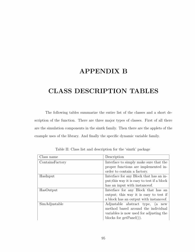
APPENDIX B
CLASS DESCRIPTION TABLES
The following tables summarize the entire list of the classes and a short de-
scription of the function. There are three major types of classes. First of all there
are the simulation components in the simtk family. Then there are the applets of the
example uses of the library. And finally the specific dynamic variable family.
Table II: Class list and description for the ‘simtk’ package
Class name Description
ContainsFactory Interface to simply make sure that theproper functions are implemented in-order to contain a factory.
HasInput Interface for any Block that has an in-put;this way it is easy to test if a blockhas an input with instanceof.
HasOutput Interface for any Block that has anoutput; this way it is easy to test ifa block has an output with instanceof.
SimAdjustable Adjustable abstract type, (a newmethod based around the individualvariables is now used for adjusting theblocks for getPanel()).
95
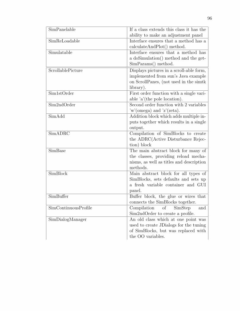
96
SimPanelable If a class extends this class it has theability to make an adjustment panel
SimReLoadable Interface ensures that a method has acalculateAndPlot() method.
Simulatable Interface ensures that a method hasa doSimulation() method and the get-SimParams() method.
ScrollablePicture Displays pictures in a scroll-able form,implemented from sun’s Java exampleon ScrollPanes, (not used in the simtklibrary).
Sim1stOrder First order function with a single vari-able ’a’(the pole location).
Sim2ndOrder Second order function with 2 variables’w’(omega) and ’z’(zeta).
SimAdd Addition block which adds multiple in-puts together which results in a singleoutput.
SimADRC Compilation of SimBlocks to createthe ADRC(Active Disturbance Rejec-tion) block
SimBase The main abstract block for many ofthe classes, providing reload mecha-nisms, as well as titles and descriptionmethods.
SimBlock Main abstract block for all types ofSimBlocks, sets defaults and sets upa fresh variable container and GUIpanel.
SimBuffer Buffer block, the glue or wires thatconnects the SimBlocks together.
SimContinuousProfile Compilation of SimStep andSim2ndOrder to create a profile.
SimDialogManager An old class which at one point wasused to create JDialogs for the tuningof SimBlocks, but was replaced withthe OO variables.

97
SimDiff Second order approximate differentia-tor defined by a Stf and is a doublepole.
SimDiffEq Difference equation which is providedfor an intermediate class as well as dis-play of the difference equation for im-plementation purposes.
SimDisturbance Disturbance sources which include fre-quency and gain variable sine andsquare waves.
SimDoubleIntegrator Directly calculated Tustin double inte-grator.
SimDoubleTriangle Double triangle profile function, whichafter integration produces an S curveprofile.
SimDTOC The DTOC(Discrete Time OptimalControl) Controller; uses two inputs,input1: error, input2: error differenti-ated.
SimDTOCDiff The DTOC algorithm with an internaldifferentiator so a single input of erroris required.
SimFactory Factory class which makes and con-trols the simulation environment bothfor the entire system and hierarchalhybrid blocks.
SimFilter Filter with a selection of multipletypes of Butterworth filters.
SimFunction Defines the bare bones of a single out-put Function block with multiple in-puts.
SimFunction2Input Defines the general class for 2 inputsand 1 output (this was replaced withthe more general SimFunction).
SimFunctionFactory Compilation internalizes the SimFac-tory into a SimFunction for complexhybrid function blocks such as NPIDcomposed from simple building blocks.

98
SimFunctionSelector Provides dynamic selection of blocksby the user at runtime; it provides alist of simulation blocks which replacesthe current block.
SimFunctionTest A test block to test internal SimFac-tory block’s.
SimFunctionXInput Multiple input SimFunction (has beenreplaced with the more general Sim-Function which can now have multipleinputs).
SimGain Simple function applies a gain to theinput.
SimGeneralClasicController A hybrid block in the general con-troller form that allows a simple con-troller with the classic ”r-y = e” inter-nally calculated to appear to a purelyerror based controller.
SimGFunc A non-linear gain function for use inshaping PID gains for NPID.
SimImage Allows a picture such as a block dia-gram to be loaded on a panel.
SimImageFactory Common utilites for loading picturesfrom files.
SimInput Defines the bare bones of a multi-input block for multi-input functionsand sinks.
SimIntegrator A directly derived Tustin integrator.SimMultiply Multiplication of two inputs with the
result at the output.SimNoise Source which after each iteration out-
puts a random value from -1 to 1.SimNothing Outputs zeros, this can be used for test
cases of zero noise instead of havingsome noise.
SimNPID Compilation of SimBlocks with acouple SimGFunc to create theNPID(Non-linear Proportional Inte-gral Derrivative) Controller.

99
SimNPIDwc Extends the SimNPID into a param-eterized PID in terms of omega for adouble integrator plant.
SimParameters Stores and keeps all the importantglobal type simulation parameterswithin this duplicated class which eachblock recieves.
SimPid Aproximate differentiator PID, this isa hybrid block composed of simplerblocks.
SimPolyProfile Provides a smoother response for po-sition, velocity, and acceleration andJerk in place of a step function ortrapezoidal function.
SimProfile A dynamically create-able profilewhich has a selection of types of in-puts(step, trapezoidal, triangle) and aselection of types of filters(integrators,2nd order, butterworth).
SimPtPlot The main plotting engine depends onthe Ptolemy PtPlot package; this addsinterfaces for plot exporting and con-nections.
SimSaturation Simple saturation function, containsand upper and lower bound limit.
SimSink Defines the bare bone nessesities to asimBlock which only has inputs.
SimSource A Bare-bones definition of a sourcewhich only has an output.
SimSourceFactory Compilation internalizes the SimFac-tory into a SimSource for complex hy-brid source blocks such as some pro-files.
SimSourceSelector Provides dynamic selection of blocksby the user at runtime; it providesa list of simulation sources which re-places the current block.

100
SimStat Provides statistical functions, such asaverage and standard deviation, on in-coming data over a specified range ofsamples.
SimStdout A sink that simply sends the currentoutput to the standard output.
SimStep A simple source Step function whichreaches a specified gain value as fastas possible.
SimStf Powerful block that simulates S do-main transfer functions and convertsthem to discrete transfer functions!.
SimSubtract Subtracts the second input from thefirst input; ”out = in1 - in2”.
SimTest A test of extending the SimFunction-Factory.
SimTextBoxOutput A sink block that simply send the cur-rent output to a formatted output ina swing text box.
SimTimeIndex Outputs the current time index whichis useful for testing blocks over a rangeof inputs.
SimTrapezoid Trapezoidal profile which can be inte-grated to provide a smother responsefor position, velocity, and accelera-tionin place of a step function.
SimTrapezoidalProfile Trapezoidal profile combined with anintegrator to form a smooth profile.
SimZtf Z domain transfer function that auto-matically creates difference equations.
SimZtfDirect A Z domain transfer functions thatcalculates the output directly with-outhanding the output down to thediffEq class.
Table III: Class list and description for the ‘simtk.applets’ package
Class name Description
ADRC GUI ADRC example applet of thesimtk library.
Console Console example of the simtk libraryto allow plot exports in non-appletmode
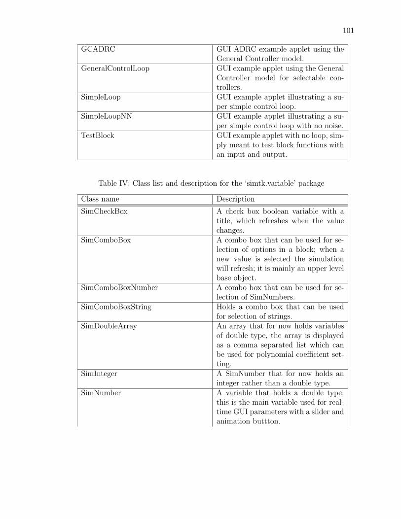
101
GCADRC GUI ADRC example applet using theGeneral Controller model.
GeneralControlLoop GUI example applet using the GeneralController model for selectable con-trollers.
SimpleLoop GUI example applet illustrating a su-per simple control loop.
SimpleLoopNN GUI example applet illustrating a su-per simple control loop with no noise.
TestBlock GUI example applet with no loop, sim-ply meant to test block functions withan input and output.
Table IV: Class list and description for the ‘simtk.variable’ package
Class name Description
SimCheckBox A check box boolean variable with atitle, which refreshes when the valuechanges.
SimComboBox A combo box that can be used for se-lection of options in a block; when anew value is selected the simulationwill refresh; it is mainly an upper levelbase object.
SimComboBoxNumber A combo box that can be used for se-lection of SimNumbers.
SimComboBoxString Holds a combo box that can be usedfor selection of strings.
SimDoubleArray An array that for now holds variablesof double type, the array is displayedas a comma separated list which canbe used for polynomial coefficient set-ting.
SimInteger A SimNumber that for now holds aninteger rather than a double type.
SimNumber A variable that holds a double type;this is the main variable used for real-time GUI parameters with a slider andanimation buttton.

102
SimStaticNumber A SimNumber that has an overloadedgetPanel() to simply display the valueof the number and not be varied by theuser.
SimString A variable that holds a string, and re-freshes the GUI when a new string isentered.
SimTest Purely a test class to test the packageand compiler paths
SimTextBox A text box variable, for display of textmaterial
SimVariable The main abstract block for all typesof SimVariables, which provides re-quirements for the reloading of theGUI mechanism.
VariableContainer A container which is used within ablock to holds each of the requiredSimVariables, from this the GUI panelis later dynamically constructed.

APPENDIX C
USER’S GUIDE
This section contains a short introduction to the usage of the simtk GUI demon-
stration applets. Again, more detailed information to the features can be found in the
javadoc documentation, but this provides a short overview of the interface structure,
peculiarities, and common troubleshooting points.
C.1 Obtain the Java Runtime Environment
In order to run the simulation package, the latest Java Runtime Environment
(JRE) from Sun is required. This can be downloaded from sun micro-systems at
http://java.sun.com, which has links to download the JRE. The JRE 1.4 was
used for the compiling and testing of this package, but it has also been successfully
compiled and run on version 1.3.
103

104
C.2 Interface Structure
The graphical user interface of the primary demonstration applet is shown in
Figure 4. There are three major sections, including the block diagram, plots, and
configurable parameters selectable via tabs. Most should be self explanatory which is
partly the purpose of GUI’s however there are a few discipline specific explanations.
C.2.1 Plots
The plots or scopes are provided through the mechanisms provided by the
PtPlot Java package. This provides navigation of the graph through smooth and
easy rectangular mouse selection to zoom in and out. Zooming in is provided by
creating a rectangle by clicking and dragging from the top to the bottom of a desired
region. Dragging from the bottom to the top zooms out.
The plot can be opened in a new window for resizing however the old window
will lose its reference to the plot. Returning to the original setup can be done by
refreshing the applet.
The PtPlot package also provide the support for exporting the plots to En-
capsulated Postscript (EPS). However, since it is saved to a file, it can not run in
applet mode. The console version of the example simtk applet can be used to save
plot outputs. To run in this mode, the Console version must be downloaded and run.
One important point to note about saving plots is the memory size of the saved files.
If the step size is too small there may be many points in the plot output resulting in
a large memory size.
C.2.2 Tabbed Blocks
Each simulation block, that is included in the simulation, is added to the list of
tabs in the upper left of the window. These tabs have a hierarchical structure; there

105
may be many tabs under a single tab. For example, a NPID block has nonlinear,
proportional, integral, and derivative tabs each separate for their own parameters.
This and Super Tabs
More advanced blocks are extensions of more primitive blocks. An advanced
block usually has some parameters that are in control of the lower level parameters.
The upper level tabs are under the default “this tab” and the lower level parameters
can be viewed under the “super tab”.
Simulation Parameters
Global values, used within many blocks, are contained within the simulation
parameters tab. This includes parameters such as step-size and final time. These are
important as global variables because some blocks reference the step-size for solver
calculations.
Diagrams
Block diagrams explain the interconnection of the blocks that make up the
selectable tabs. A few of the controllers have a tab called “diagram” that is available
to display the interconnection of the controller. Combined with the overall diagram
this can show the full structure of the system.
C.2.3 Parameters
Parameters are the dynamic adjustable variables that can be varied in real-
time to adjust design. There are a couple of main types of parameters; each have
their own graphical user interface methods.
Some parameters may not be able to be adjusted if there is an upper level

106
parameter. In this case the parameter will simply remain the same and is only
available for viewing.
Numbers
Numbers are the most common parameter type. These are adjusted by sliders
and text fields. The sliders behave in an exponential varying manner. A slider can
vary the value of a number by a magnitude of 4 up or down. Each time the slider
is released the new value becomes the center point. The center point can also be
manually reset via a text box which requires a <CR> Carriage Return to refresh the
simulation with the new value.
A recent addition to the package is a small check box next to a slider of a
number variable. This button puts the simulation into animation mode which swings
the variable slider back and forth around the last set point to automatically view the
changes. This is a valuable feature to allow varying multiple parameters at the same
instant. The computer can automatically vary a parameter while the user manually
adjusts another. Selecting the animation buttons becomes taxing on the processing
power of a computer. If too many animation buttons have been selected, the refresh
rate of the simulation can be significantly reduced.
Arrays
Arrays are comma delimited numbers. These are used in functions such as
transfer functions for the S domain and Z domain with class titles of SimStf and
SimZtf respectively.
For example, a Stf numerator array of coefficients
1, 2, 3, 4

107
Would result in a Laplace polynomial of
s3 + 2s2 + 3s + 4 (C.1)
This is similar to the format that both Matlab and SysQuake use to define transfer
functions.
C.3 Example Usage Steps and Tips
The following is an ordered list of the steps to take when using the example
controls applet for the simtk library.
1. Open applet from a web page1 or a local disk
2. Select and modify a plant under the plant tab
3. Select an input reference (usually a step or a profile is used as an appropriate
reference)
4. Select a controller under the controller tab
5. Adjust the final time and simulation step size to match the design requirements
as well as an appropriate refresh rate. If the product of final time and step size
is too large, the computer might not be able to simulate in “real-time” for each
parameter update.
6. Select noises and disturbances to test the stability of the selected controller for
the selected plant.
7. If the controller is parameterized, adjust the bandwidth of the controller along
with the bandwidth of the reference profile to appropriately control the system.
1The applet is currently available at http://academic.csuohio.edu/aerl/simtk/

108
C.4 Troubleshooting
There are a few common troubleshooting points that are addressed in the
following sections.
Slow Update Time or Frozen Interface
If the product of final time and step size is too large, the computer might not
be able to simulate every iteration quick enough to appear real time. Try reducing
the simulation step-size, final time or both.
Large Plot Exports
If the step size is too small, there may be many points in the plot output
resulting in a large memory size.
Entering a Transfer Function
For now, the transfer functions are limited to 4th order. If the plant has an
order greater than this, two transfer functions can be cascaded to produce the required
order.

APPENDIX D
ADDITIONAL FIGURES
There are additional figures that, while not strictly important to be included
in the core of the document, could prove useful for future information.
D.1 Inheritance Structure
The following are some additional figures to complement the figures from Chap-
ter 2.
109

110
Scrollable
ScrollablePictureJLabel
SimPanelable
Sim1stOrder
Sim2ndOrder
SimADRCSimFunctionFactory
SimContinuousProfile
SimSourceFactory
SimDiff
SimStf
SimDiffEq
SimDisturbance
SimDoubleTriangle
SimDTOC SimDTOCDiff
SimFactory
SimFilter
SimFunctionSelector SimFunctionTest
SimGain
SimGeneralClasicControllerSimGFunc
SimImage
SimNoise
SimNothing
SimNPID
SimParameters
SimPid
SimPolyProfile
SimProfile
SimPtPlot
SimSaturation
SimSourceSelector
SimStat
SimStep
SimTest
SimTextBoxOutput
SimTimeIndex
SimTrapezoid
SimTrapezoidalProfile
SimZtf
SimDoubleIntegrator
SimIntegrator
SimFunction
SimAdd
SimSubtract
SimZtfDirect
SimBase
SimBlock
SimBuffer
SimSourceSimInput
SimFunction2Input
SimFunctionXInput
SimDialogManager
Iterator
Simulatable
HasOutput
SimSink
SimMultiply
JApplet SimImageFactory
HasInput
SimNPIDwc
SimStdout
Figure 32: The class structure for the blocks

111
JLabel ScrollablePicture
SimZtf
Sim1stOrder
Sim2ndOrder
SimStf
SimDoubleIntegrator
SimIntegratorSimFunction
SimAdd
SimFunctionFactory
SimDiffEq
SimDTOC
SimFunctionSelector
SimGain
SimGFunc
SimSaturation
SimStat
SimSubtract
SimZtfDirect
SimADRC
SimDTOCDiff
SimFunctionTest
SimGeneralClasicController
SimNPID
SimTest
SimBase
SimBlock
SimParameters
SimBuffer
SimSource
SimFactory
SimInput
SimFunction2Input
SimFunctionXInput
SimImage
SimSourceFactory SimContinuousProfile
SimProfile
SimTrapezoidalProfile
SimDialogManager
SimDiff
SimFilter
SimPid
SimDisturbance
SimDoubleTriangle
SimNoise
SimNothing
SimPolyProfile
SimSourceSelector
SimStep
SimTimeIndex
SimTrapezoid
SimSink
SimMultiply
JApplet SimImageFactory
SimNPIDwc
SimPtPlot
SimStdout
SimTextBoxOutput
Figure 33: The entire hierarchical class structure of the project (without implemen-
tation classes)
SimVariable
SimCheckBox
SimComboBox
SimDoubleArray
SimNumber
SimString
SimTextBox
SimComboBoxNumber
SimComboBoxString
SimInteger
SimStaticNumber
SimTest
SimPanelable VariableContainer
SimBase
Iterator
Figure 34: The class structure for the dynamic variables

112
Simulatable ADRC
Console
GCADRC
GeneralControlLoop
SimpleLoop
SimpleLoopNN
TestBlockJApplet
implements
Figure 35: The applet class structure
SimVariable
SimCheckBox
SimComboBox
SimDoubleArray
SimNumber
SimString
SimTextBox
SimComboBoxNumber
SimComboBoxString
SimInteger
SimStaticNumber
SimTest
SimBase
VariableContainer
Figure 36: The class structure for the dynamic variables (without implementation
classes)

113
JApplet
ADRC
GCADRC
GeneralControlLoop
SimpleLoop
SimpleLoopNN
TestBlock
implements Console
Figure 37: The applet class structure (without implementation classes)

114
D.2 Containment Structure
The following are some additional figures to complement the figures from Chap-
ter 3.
The un-simplified, entire containment of the classes for the GeneralControl-
Loop applet is illustrated in Figure 38.
ContainsFactory
HasInput
SimBufferHasOutput
ScrollablePicture
Sim1stOrder
SimZtf
SimNumber
SimDoubleArray
SimCheckBox
Sim2ndOrder
SimADRC
SimFunctionFactory
SimStf
SimPtPlot
SimSubtract
SimIntegrator
SimFunction
SimFactory
SimInput
SimImage
Simblock
SimSink
Simple
SimAdd
SimAdjustable
SimStep
SimReLoadable
SimSource
SimBase
Simulatable
SimParametersSimBlock
SimDialogManager
GeneralControlLoop
SimBlocks
SimField
SimParameter
SimContinuousProfile
SimSourceFactory
SimDTOCSimDTOCDiff
SimDiff
SimPid
SimDiffEq
SimTextBox
SimDisturbance
SimComboBoxString
SimDoubleIntegrator
SimDoubleTriangle
SimPanelable
Simulation
SimTabBox
SimFilter
SimFunction2Input
SimFunctionSelector
SimFucntionSelector
SimFunctionTest
SimGain
SimFunctionXInput
SimGFunc
SimGeneralClasicController
SimImageFactory
SimMultiply
SimNPID
SimNPIDwc
SimNoise
SimNothing
SimPolyProfile
SimProfile
SimSourceSelector
SimSaturation
SimStat
SimInteger
SimStaticNumber
SimComboBoxNumber
SimStdout
SimTest
SimTextBoxOutput
SimTimeIndex
SimTrapezoid
SimTrapezoidalProfile
SimZtfDirect
Figure 38: Example Containment of classes for the GeneralControlLoop applet
D.3 Screen Shots
A screen shot of an early version of the GUI for the sample applet of the simtk
library applet is shown in Figure 39.

115
Figure 39: Early screen shot for the simtk applet GUI
The structure is rather confusing and a more organized view is shown in Fig-
ure 40.

116
Figure 40: Early organized screen shot for the simtk applet GUI
The current screen shot for the sample simtk applet GUI is shown in Figure 4
in Chapter 2.

APPENDIX E
SAMPLE CODE
Due to the amount of source code for the project a few of the important code
listings are cited here. The entire source can be obtained from the web site or from
a CD-ROM.
Listing E.1: GeneralControlLoop applet example of library use/∗
<app l e twidth=”1000”he i gh t=”600”code=”simtk . a pp l e t s . GeneralControlLoop . c l a s s ”codebase =” . ./ . . /”arch i ve=”ptolemy/ p l o t / p l o t a p p l e t . j a r ”a l t=”Your browser understands the & l t ;APPLET> ;tag but i sn ’ t running the app le t , f o r some reason .”>
</app le t>∗Fri May 3 12 :18 :40 EDT 2002∗/package simtk . app l e t s ;
// import ptolemy . p l o t . ∗ ;import simtk . ∗ ;import javax . swing . ∗ ;import java . awt . ∗ ;/∗∗∗ Sample o f the javasim l i b r a r y∗ @author Aaron Radke∗ t i t l e : GeneralControlLoop∗ <br>∗ author : Aaron Radke∗ <br>∗ date :2/5/03∗ <br>∗ ab s t r a c t : Sample o f the javasim l i b r a r y making use o f the genera l c l a s s i c a l∗ con t ro l s t r u c t u r e so any a lgor i thm with any p lan t can be s e l e c t e d !∗/
117

118
public class GeneralControlLoop extends JApplet implements Simulatab le {/∗ ∗ Return a s t r i n g d e s c r i b i n g t h i s app l e t . ∗/public St r ing getApp le t In fo ( ) {
return ”by Aaron Radke in AERL\n” ;}/∗∗∗ I n i t i a l i z e the app l e t . Here we s t ep through an example o f what the∗ the app l e t can do .∗/
// s imu la t ion parametersSimParameters params = new SimParameters ( ) ;// g i v e the f a c t o r y the se parametersSimFactory f a c t o r y = new SimFactory ( params ) ;
public void i n i t ( ) {super . i n i t ( ) ;s imu l a t i o n i n i t ( ) ;
}//end of i n i t ( )
public SimParameters getSimParams ( ){return params ;
}
void s imu l a t i o n i n i t ( ){f a c t o r y . setReloadBlock ( this ) ;params . setReloadBlock ( this ) ;
// i n s t a n t i a t e s imb locks// crea t e some b l o c k s to p lay withSimTextBoxOutput textout= new SimTextBoxOutput ( ) ;
SimPtPlot outputscope = new SimPtPlot ( ) ;outputscope . setHidden ( true ) ;
SimImage image = new SimImage ( ) ;image . setFileName ( ” ad r c c l o s ed l o op . g i f ” ) ;image . setHidden ( true ) ;
SimSubtract feedbacksub = new SimSubtract ( ) ;S imFunct ionSe lector fsC = new SimFunct ionSe lector ( ) ;
fsC . cb . setValue ( S imFunct ionSe lector .GAIN) ;S imFunct ionSe lector fsP = new SimFunct ionSe lector ( ) ;
fsP . cb . setValue ( S imFunct ionSe lector . INT ) ;SimStep step = new SimStep ( ) ;S imSourceSe lector t s t ep = new SimSourceSe lector ( ) ;SimGain rga in = new SimGain ( ) ;SimGain ygain = new SimGain ( ) ;S imSourceSe lector ssR = new SimSourceSe lector ( ) ;S imSourceSe lector ssN = new SimSourceSe lector ( ) ;
ssN . cb . setValue ( S imSourceSe lector .NOTHING) ;S imSourceSe lector ssD = new SimSourceSe lector ( ) ;
ssD . cb . setValue ( S imSourceSe lector .NOTHING) ;SimADRC adrc = new SimADRC( ) ;
SimAdd distAdder = new SimAdd ( ) ;SimAdd noiseAdder = new SimAdd ( ) ;S imGenera lC la s i cCont ro l l e r genc = new S imGenera lC la s i cCont ro l l e r ( ) ;
// // s e t s imb lock i n i t i a l va lue sparams . setParameters ( 1 0 , 0 . 1 , 4 ) ;
//// //================== facory add api// // f a c t o r y . add ( outputb lock , ” output b l o c k t i t l e ” , i npu t b l o c k ) ;// //−−−−−−−−−−−−−
SimSource r e f = ssR ; //ssRSimFunction c o n t r o l l e r = genc ; //adrc ;// genc ;// fsCSimFunction p lant = fsP ; // fsPSimSink output = textout ;SimSource p l a n t d i s t = ssD ; //ssRSimSource s e n s n o i s e = ssN ; //ssR
f a c t o r y . add ( image , ” ImageBlock” ) ;

119
f a c t o r y . add ( r e f , ” input ” ) ;f a c t o r y . add ( p l an t d i s t , ”Plant Disturbance ” ) ;f a c t o r y . add ( distAdder , ” d i s turbance adder ” , c o n t r o l l e r , p l a n t d i s t )f a c t o r y . add ( plant , ”Plant ” , distAdder ) ;f a c t o r y . add ( s en s no i s e , ” Sesnor Noise /Disturbance ” ) ;f a c t o r y . add ( noiseAdder , ” output no i s e adder ” , plant , s e n s n o i s e ) ;// f a c t o r y . add ( output ,” Output Text ” , p l an t ) ;f a c t o r y . add ( outputscope , ”Output Scope” , r e f ) ;
outputscope . addLegend (0 , ” Reference ” ) ;outputscope . addInput ( p lant ) ;outputscope . addLegend (1 , ”Plant output ” ) ;outputscope . addInput ( c o n t r o l l e r ) ;outputscope . addLegend (2 , ” Con t r o l l e r Output” ) ;
//e = r−y // re f−p lan t to c o n t r o l l e rf a c t o r y . add ( c on t r o l l e r , ”General Con t r o l l e r ” , r e f , noiseAdder ) ;//−−−−−−−−−−−−−−−−//−−−add the f a c t o r y to the content pane//−−−−−−−−−−−−−−−−Container cp = getContentPane ( ) ; // d e f a l u t i s border l ayou t//Create a s p l i t pane with the two s c r o l l panes in i t .JSpl i tPane horzSpl i tPane = new JSpl i tPane ( JSpl i tPane .HORIZONTAL SPLIT,
f a c t o r y . getPanel ( ) , outputscope . getPanel ( ) ) ;horzSpl i tPane . setOneTouchExpandable ( true ) ;horzSpl i tPane . s e tD iv ide rLoca t i on ( 2 5 0 ) ;
JSpl i tPane ver tSp l i tPane = new JSpl i tPane ( JSpl i tPane .VERTICAL SPLIT,horzSpl i tPane , image . getPanel ( ) ) ;
ve r tSp l i tPane . setOneTouchExpandable ( true ) ;ve r tSp l i tPane . s e tD iv ide rLoca t i on ( 4 2 0 ) ;
cp . add ( BorderLayout .CENTER, ver tSp l i tPane ) ; // put f a c t o r y and p l o t in centercp . add ( BorderLayout .NORTH,new JLabel (
”Genearl Control System” ,SwingConstants .CENTER) ) ; // put but ton b l o c k s on the bottom
doSimulat ion ( ) ;}//end of s imu la t ion i n i t
/∗∗ t h i s i s not r e a l l y used anymore???∗/public void doSimulat ion ( ){
f a c t o r y . doSimulat ion ( ) ;}
}//end
Listing E.2: 2nd Order function example of adding to the librarypackage simtk ;import simtk . v a r i a b l e . ∗ ;import java . u t i l . ∗ ;import javax . swing . ∗ ;/∗ ∗ (wˆ2)/( s ˆ2 + 2∗w∗ z∗ s + wˆ2)∗∗/public class Sim2ndOrder extends SimZtf implements SimPanelable{
/∗∗omeaga i s w as in∗ (wˆ2)/( s ˆ2 + 2∗w∗ z∗ s + wˆ2)∗/SimNumber omega = new SimNumber( ”Omega ( Bandwidth ) ” , 1 ) ;/∗∗ z e ta i s z as in∗ (wˆ2)/( s ˆ2 + 2∗w∗ z∗ s + wˆ2)∗/SimNumber zeta = new SimNumber( ”Zeta (Damping c o e f f i c e n t ) ” , 1 ) ;/∗∗ cons t ruc tor s e t omeag = 1 and ze ta = 1∗ (wˆ2)/( s ˆ2 + 2∗w∗ z∗ s + wˆ2)∗ s e t a to 1 so d e f a u l t o f 1/( s+a ) i s 1/( s+1)∗/public Sim2ndOrder ( ){
s e tT i t l e ( ”2nd order ” ) ;s e tDe s c r i p t i on ( ”2nd order c r i t i c a l l y damped” ) ;ge tVar iab l eConta iner ( ) . add (omega ) ;ge tVar iab l eConta iner ( ) . add ( zeta ) ;
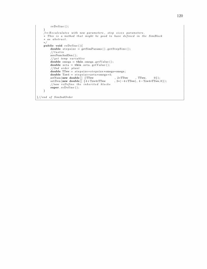
120
r eDe f ine ( ) ;}/∗∗Reca l cu l a t e s with new parameters , s t ep s i z e s parameters .∗ This i s a method tha t might be good to have de f ined in the SimBlock∗ as a b s t r a c t .∗/public void r eDe f ine ( ){
double s t e p s i z e = getSimParams ( ) . g e tS t epS i z e ( ) ;// t u s t i nzeroNumAndDen ( ) ;// ge t temp v a r i a b l e sdouble omega = this . omega . getValue ( ) ;double ze ta = this . z e ta . getValue ( ) ;//2nd order p l an tdouble TTww = s t e p s i z e ∗ s t e p s i z e ∗omega∗omega ;double Tzw4 = s t e p s i z e ∗ ze ta ∗omega ∗4 ;setNum(new double [ ] {TTww , 2∗TTww , TTww, 0} ) ;setDen (new double [ ] {4+Tzw4+TTww , 2∗(−4+TTww) , 4−Tzw4+TTww, 0 } ) ;//now reDef ine the i n h e r i t e d b l o c k ssuper . r eDe f ine ( ) ;
}
}//end of Sim2ndOrder
INDEX
aaindex, 93
aao.vim, 93
aao2dot, 94
aao2pdf, 93
aao2tex, 93
ACAD, 83
ADRC, 46, 64, 81
algorithms, 28
API, 17
Application Programmers Interface, 17
auto-tuning, 66
Automated Computer Assisted Design,
83
bandpass, 57
bandstop, 57
Bilinear, 28
butterworth, 56
classical representation, 62
Coefficient of Variation, 74
coefficient of wavelet variation, 77
compressgif, 94
containment, 93
containment.pl, 21
Continuous Time Optimal Control, 49
control system, 61
COV, 74
csuthesis.sty, 94
CTOC, 49
developers, 19
difference equation, 12, 39
differential equation solvers, 27
differentiator, 68
discrete, 6
DTOC, 48, 81
Encapsulated Postscript, 104
engineering requirements, 67
EPS, 104
ESO, 46
Euler, 32
Extended State Observer, 46
extractClassInfo, 94
filters, 51
Fundamental building blocks, 12
Gao, 83
general controller block, 62
general feedback system, 62
121

122
general representation, 62
Gnuplot, 12, 91
Graphical User Interface, 3
Graphviz, 92
GUI, 3, 17
GUIDE, 90
Hartmath, 92
HasFactory, 21
high-pass, 57
improved general controller block, 63
Java, 7, 90
Java code
s2z, 38
z2d, 40
java2dot, 13, 93
Least Mean Square, 75
linear regression, 75
LMS, 75
low-pass, 57
MacOS, 7
Maple, 2
Mathematica, 2, 90
Matlab, 2, 3, 90
maximum sample, 71
minimum sample, 71
Most Significant Bandwidth Threshold,
69
MSBT, 69
noise, 67
NPID, 4, 81
object-oriented, 12
Octave, 91
ode45, 27
OO, 12
optimization threshold, 67
optimized
actively, 66
overshoot, 69
Parameterization, 42
Perl, 12, 91
PID, 2, 42, 63
pre-filters, 51
profiles, 51
proportional-integral-derivative, 42
Ptolemy, 91
PtPlot, 7
quantifying noise, 70
rate of change, 68
Runge-Kutta, 30, 32
123
s-functions, 4
s2z, 36
SimBlocks, 13
SimBuffer, 17
SimFactory, 17, 20
SimFunction, 13
Simple Euler, 28
SimSink, 13
SimSource, 13
Simulink, 3
standard deviation, 73
steady-state, 71
SysQuake, 2, 4, 90
Time Optimal Control, 70
Trapezoidal, 28, 51
Tustin, 28
University of British Columbia, 28
Unix, 7
users, 19
variance, 73
Vim, 92
wavelet, 77
wavelet variance, 77
Windows, 7
Wolfram, 90
z2d, 39
Zero Order Hold, 82