a joint monte carlo analysis of seafloor compliance ...noise.earth.utah.edu/ggge20616.pdf · ously...

TECHNICAL BRIEF10.1002/2014GC005412

A joint Monte Carlo analysis of seafloor compliance, Rayleighwave dispersion and receiver functions at ocean bottomseismic stations offshore New ZealandJustin S. Ball1, Anne F. Sheehan1, Joshua C. Stachnik2, Fan-Chi Lin3, and John A. Collins4

1CIRES and Department of Geological Sciences, University of Colorado at Boulder, Colorado, USA, 2Department of Earthand Environmental Sciences, Lehigh University, Bethlehem, Pennsylvania, USA, 3Department of Geology and Geophysics,University of Utah, Salt Lake City, Utah, USA, 4Department of Geology and Geophysics, Woods Hole Oceanographic Institu-tion, Woods Hole, Massachusetts, USA

Abstract Teleseismic body-wave imaging techniques such as receiver function analysis can be notori-ously difficult to employ on ocean-bottom seismic data due largely to multiple reverberations within thewater and low-velocity sediments. In lieu of suppressing this coherently scattered noise in ocean-bottomreceiver functions, these site effects can be modeled in conjunction with shear velocity information fromseafloor compliance and surface wave dispersion measurements to discern crustal structure. A novel tech-nique to estimate 1-D crustal shear-velocity profiles from these data using Monte Carlo sampling is pre-sented here. We find that seafloor compliance inversions and P-S conversions observed in the receiverfunctions provide complimentary constraints on sediment velocity and thickness. Incoherent noise inreceiver functions from the MOANA ocean bottom seismic experiment limit the accuracy of the practicalanalysis at crustal scales, but synthetic recovery tests and comparison with independent unconstrained non-linear optimization results affirm the utility of this technique in principle.

1. Introduction

The seafloor is a challenging environment for seismologists. Noise presents a significant obstacle to the oceanbottom seismometer (OBS) analyst. A diverse range of physical processes in the ocean and solid Earth generateseismoacoustic energy across a wide spectrum ranging from tidal periods to the microseism band and above[Crawford et al., 1991; Godin and Chapman, 1999]. This ‘‘rich wavefield’’ [Ritzwoller and Levshin, 2002] recorded onseafloor seismometers can be either vexatious or auspicious to the investigator, depending on the task at hand.

Body-wave methods utilizing horizontal-component information such as shear-wave splitting and receiverfunctions are particularly difficult with OBS data. High-amplitude current-induced tilt noise is often observedon OBS horizontal channels [Webb, 1998], and a ubiquitous diffuse infragravity wavefield is recorded on allcomponents at periods greater than about 40 s [Crawford et al., 1991; Webb, 1998; Willoughby and Edwards,2000]. Between 2 and 10 s period, microseismic noise prevails [Webb, 1998], and at infrasonic frequenciesabove 5 Hz hydroacoustic phases can be prevalent. Simple filtering is not always effective in improving OBSdata quality due to this diverse noise spectrum.

At typical OBS sites, even high signal-to-noise ratio (SNR) events are distorted by reverberations in the waterand shallow sediment columns that overprint deeper arrivals in the receiver function [Leahy et al., 2010].Large volumes of low shear-velocity marine sediments can also impose delays in teleseismic traveltimesthat necessitate static corrections [Harmon et al., 2007]. Mitigating these effects is a subject of active interestin the marine seismology community.

The seafloor noise wavefield can be utilized to elucidate velocity structure. Ambient Noise Tomography(ANT) of Rayleigh waves effectively resolves group and phase velocity dispersion at periods from 6 to 27 s,which can be inverted for shear-velocity structure [Lin et al., 2007]. In similar fashion, the seafloor’s responseto loading by infragravity waves (the seafloor compliance) from 50 to 250 s also depends on the shearvelocity structure beneath the OBS [Crawford et al., 1991; Willoughby and Edwards, 2000]. Observed shearresonances in the sediment column excited by ambient noise can also constrain shallow sediment velocities[Godin and Chapman, 1999].

Key Points:� Joint inversion for seafloor

compliance, receiver functions, andsurface waves� Application to real data problematic

due to reverberations on receiverfunctions� Sediment properties constrained by

seafloor compliance and receiverfunctions

Correspondence to:J. S. Ball,[email protected]

Citation:Ball, J. S., A. F. Sheehan, J. C. Stachnik,F.-C. Lin, and J. A. Collins (2014), A jointMonte Carlo analysis of seafloorcompliance, Rayleigh wave dispersionand receiver functions at oceanbottom seismic stations offshore NewZealand, Geochem. Geophys. Geosyst.,15, 5051–5068, doi:10.1002/2014GC005412.

Received 21 MAY 2014

Accepted 4 NOV 2014

Accepted article online 8 NOV 2014

Published online 17 DEC 2014

BALL ET AL. VC 2014. American Geophysical Union. All Rights Reserved. 5051

Geochemistry, Geophysics, Geosystems

PUBLICATIONS

http://dx.doi.org/10.1002/2014GC005412

http://onlinelibrary.wiley.com/journal/10.1002/(ISSN)1525-2027/

http://publications.agu.org/

In this paper, we combine the shear velocity information obtained from the ambient noise observations(dispersion and compliance) with receiver functions in hopes of teasing out crustal arrivals obscured bysediment reverberations in the receiver functions, with application to OBS data from offshore New Zealand.

1.1. MOANA Experiment and Geologic SettingThe Marine Observations of Anisotropy Near Aotearoa (MOANA) experiment included the deployment of 30broadband OBS and Differential Pressure Gauges (DPG) off both east and west coasts of the South Island ofNew Zealand from 2009 to 2010 (Figure 1) [Yang et al., 2012]. The purpose of MOANA is to characterize therheological controls on upper mantle deformation and its spatial extent in the region using observations ofanisotropy as a strain gauge [Zietlow et al., 2014; Collins and Molnar, 2014].

The MOANA stations off the South Island’s East coast are situated in and around the inner Bounty Trough, aCretaceous extensional basin containing thick deposits (up to 6 km) of terrigenous and marine sediments.Prior studies estimate crustal thicknesses of 18–25 km beneath the Eastern MOANA array and suggest thepresence of a seismically fast, thin (�3 km) lower crustal layer [Scherwath et al., 2003; Van Avendonk et al.,2004] of possibly relict oceanic crust.

The Western MOANA array is mostly situated on the Challenger Plateau, an area of relatively undeformedsubmerged continental crust of the Australian plate estimated to range in thickness from 18 to 27 km

Figure 1. Map showing topography and bathymetry on and surrounding South Island of New Zealand. Yellow triangles represent ocean-bottom seismographs (OBS) deployed during the MOANA experiment. Purple triangles are land stations deployed during the same experi-ment. Red triangles are permanent GeoNet stations. OBS stations NZ16 and NZ06 are analyzed in this paper. Red circles show IODP bore-holes used to ground-truth the analysis.

Geochemistry, Geophysics, Geosystems 10.1002/2014GC005412


beneath the MOANA OBS sites[Scherwath et al., 2003; Van Aven-donk et al., 2004; Wood and Wood-ward, 2002]. A layer of high-grademetamorphic rock in the lowercrust beneath the plateau ispostulated to be responsible forhigh lower-crustal velocitiesobserved in active-source studiesoff the West coast [Scherwathet al., 2003]. Sediment thicknessesbeneath the Western array areestimated from sonobuoy andseismic reflection data to rangefrom 460 to 800 m [Divins, 2003].The gravity modeling of Woodand Woodward [2002] estimatessediment thicknesses to be1–3 km in the same locationsassuming constant densities inthe sediment and basement of2.33 and 2.78 g/cm3, respectively.

In 1975, leg 29 of the Deep SeaDrilling Project (DSDP) took sedi-

ment core samples from site 284 on the Challenger Plateau at a distance of �100 and �160 km from sta-tions NZ06 and NZ16, respectively. They recovered a 200 m section of homogeneous calcareous oozelacking in detrital minerals and terrigenous sediments and dating to the late Miocene at depth. Sonic logsof the core yield a bulk average Vp of 1.57 6 0.02 km/s. The core did not penetrate to basement rock andbased on shipboard sub bottom profiler data sediment thickness was estimated to exceed 600 m [Kennettet al., 1975].

2. Data

The analyses presented below reveal information about absolute subsurface S-velocities (via Rayleigh-wavedispersion, seafloor compliance) and the trade-off between bulk velocities and interface depths (via receiverfunctions). These data are forward-modeled over thousands of realizations of randomly perturbed modelstates via a Markov Chain Monte Carlo (MCMC) algorithm [Haario et al., 2006] (section 3) to produce a suiteof model realizations fitting the data to within a user-specified tolerance. In this section, we describe thedata that go into our MCMC algorithm.

2.1. OBS Receiver Function EstimationTeleseismic receiver functions are estimates of the near-receiver shear-wave impulse-response to an inci-dent P-wave, and are obtained by deconvolving the radial component seismogram by the vertical compo-nent (a proxy for the source-time function) [e.g., Langston, 1979; Owens et al., 1988]. We calculate receiverfunctions from the MOANA experiment OBS data using earthquakes of mb>6.0 and the epicentral distancerange of 20–100� (Figure 2). A total of 93 events were found to fit these criteria, and low-SNR events weremanually culled on a per-station basis. An extensive variety of frequency passbands were evaluated. In thisstudy, we utilize a passband of 0.5–5 Hz for sedimentary layer analysis, and 0.05–2.5 Hz for deeper crustaland Moho analysis.

We use the multitaper spectral correlation algorithm of Park and Levin [2000] to produce the receiver func-tion stacks employed in this analysis (Figure 3). This method produces coherence-weighted stacks in epi-central distance bins, suppressing random noise by stacking multiple receiver functions in the frequencydomain. Since the majority of high-SNR teleseisms recorded by MOANA are clustered in epicentral distanceranges of �30 and �90� , only bin-averaged receiver functions from these distances were employed in this

Figure 2. Distribution of earthquakes used in receiver function analysis. Analysis wasrestricted to earthquakes with magnitudes greater than 6.0 and epicentral distances of20 100� . A total of 93 events were found to fit these criteria.



(a)

(b)

Figure 3. (a) Radial (left) and tangential (right) receiver function stacks for station NZ16, binned by epicentral distance andstacked with weight determined from vertical-horizontal coherence (see text for details). Azimuthal smoothing is applied via 10�

overlap in epicentral bins. Positive arrivals are shown in blue, negative in red. The RF stack from the 30� bin was employed inthis analysis because it contains the greatest number of high-SNR teleseisms. (b) Radial (left) and tangential (right) receiver func-tion stacks for station NZ06. As in Figure 3a, the RF stack from the 30� bin was used due to the large number of high-SNR eventsit contains.



study. Average estimated slownesses corresponding to these distance ranges were incorporated into theforward modeling of receiver functions by the Monte Carlo algorithm.

2.1.1. Sediment Effects on OBS Receiver FunctionsGeneral features of receiver functions in marine sediments are common to those observed in sedimentarybasins on land [Het�enyi et al., 2006; Langston, 2011; Park and Levin, 2000]. The dominant early mode-converted arrivals observed in MOANA receiver functions result from shallow impedance contrasts in thesediments (Figure 3). Very large shear velocity contrasts are possible across the sediment-basement contact[Godin and Chapman, 1999; Harmon et al., 2007] giving rise to a strong pulse in the receiver functions atdelay times of �1 s (depending on sediment thickness). These strong early pulses are the most coherentfeature in MOANA receiver function waveforms across all epicentral distance bins (Figure 3). The free sur-face of the ocean is a near-perfect reflector for upgoing P waves in the water column, causing water multi-ples to be observed on OBS receiver functions [Bostock and Trehu, 2012]. Crustal multiples andunambiguous Moho-converted arrivals are not clearly observable in MOANA receiver functions.

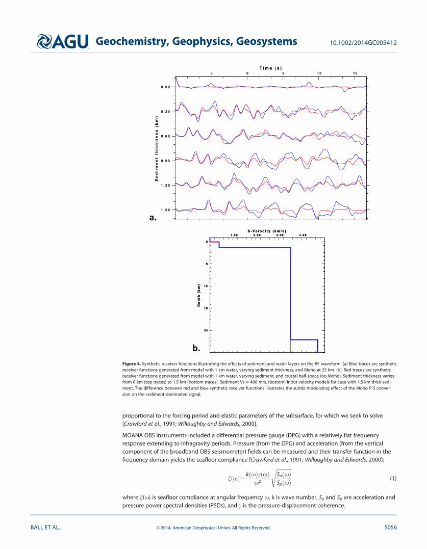
We investigated the relative contributions of water and sediment multiples to receiver function amplitudesusing synthetic seismograms [Herrmann and Ammon, 2004; Herrmann, 2013] (Figure 4). As model sedimentthickness is increased, the sediment-basement P-S converted arrival is observed at later times, as expected.The interference behavior between sediment, water, and crustal reverberations is complex and highly sensi-tive to sediment properties. Figure 4 illustrates the subtle modulation of the dominantly sediment-controlled receiver function signal by the Moho-converted shear-wave arrival that we seek to resolve in thisanalysis. The red traces in Figure 4 are computed for a model with water and sediments over a crustal-velocity half-space, and the blue traces are for a model with water, sediments, and a crustal layer over amantle half-space (i.e., blue trace is for a model with a Moho, red trace does not have a Moho). The differ-ence between the two reflects the small magnitude of Moho P-S conversion and reverberations that wehope to resolve from beneath the sediment signal.

2.2. Absolute S-Velocity EstimationAbsolute shear velocity information is estimated from Rayleigh-wave dispersion and seafloor complianceand is used to better model the sediment reverberations in the receiver functions. Both surface wave dis-persion and seafloor compliance are determined using recordings of ambient noise.

2.2.1. Rayleigh DispersionOBS sites are relatively quiet at periods in the ‘‘noise notch’’ from �10 to 30 s [Crawford et al., 1991; Webb,1998; Willoughby and Edwards, 2000], allowing robust seafloor Rayleigh dispersion curves to be estimated inthis band [e.g., Forsyth et al., 1998; Ye et al., 2013]. Rayleigh waves at these periods are most sensitive tovelocity structure from approximately 15–45 km depth. Group velocity dispersion from ambient noisetomography following the method of Stachnik et al. [2008] and phase velocity dispersion derived fromearthquakes and ambient noise [Lin et al., 2008, 2009] were determined using frequency-time analysis. Theambient noise tomography employed stacked one-bit normalized cross-correlations of hourly data windowsbetween all station pairs. The resulting phase and group velocity maps were sampled at MOANA stationlocations to produce the dispersion curves presented here.

To estimate starting models in agreement with our Rayleigh dispersion data, we first performed a damped,linearized inversion of dispersion measurements from MOANA OBS stations. Group and phase velocity dis-persion at each station was inverted for shear velocity models using the surf96 software from the CPS330package of Herrmann and Ammon [2004]. This software performs a damped, linearized least-squares inver-sion for shear velocities in a stack of discrete layers.

The inversion was performed using a fixed-velocity water layer and a constant-velocity starting model(Vs 5 4.7 km/s). The algorithm then solves for Vs in a stack of layers of increasing thickness from 1–10 kmwith depth, and the results are used to formulate starting models for the Monte Carlo analysis.

2.2.2. Seafloor ComplianceThe nonlinear interaction of ocean surface gravity waves generates propagating infragravity-band (50–250 s) waves that attenuate very little on a basin-wide scale due to their long wavelengths (10–50 km)[Webb, 1998]. Infragravity waves excite evanescent displacements on the seafloor with depth sensitivity



proportional to the forcing period and elastic parameters of the subsurface, for which we seek to solve[Crawford et al., 1991; Willoughby and Edwards, 2000].

MOANA OBS instruments included a differential pressure gauge (DPG) with a relatively flat frequencyresponse extending to infragravity periods. Pressure (from the DPG) and acceleration (from the verticalcomponent of the broadband OBS seismometer) fields can be measured and their transfer function in thefrequency domain yields the seafloor compliance [Crawford et al., 1991; Willoughby and Edwards, 2000]:

nðxÞ5 kðxÞcðxÞx2

ffiffiffiffiffiffiffiffiffiffiffiffiSaðxÞSpðxÞ

s(1)

where n(x) is seafloor compliance at angular frequency x, k is wave number, Sa and Sp are acceleration andpressure power spectral densities (PSDs), and c is the pressure-displacement coherence.

Figure 4. Synthetic receiver functions illustrating the effects of sediment and water layers on the RF waveform. (a) Blue traces are syntheticreceiver functions generated from model with 1 km water, varying sediment thickness, and Moho at 25 km. (b). Red traces are syntheticreceiver functions generated from model with 1 km water, varying sediment, and crustal half-space (no Moho). Sediment thickness variesfrom 0 km (top traces) to 1.5 km (bottom traces). Sediment Vs 5 400 m/s. (bottom) Input velocity models for case with 1.5 km thick sedi-ment. The difference between red and blue synthetic receiver functions illustrates the subtle modulating effect of the Moho P-S conver-sion on the sediment-dominated signal.



We estimated seafloor compliance for the MOANA stations using stacked multitaper power spectral den-sities computed for hour-long sliding windows over 24 h data segments encompassing 120 days of continu-ous data. Windows containing earthquakes or transients were rejected automatically based on their lowpressure-vertical coherence.

Subsequently a gain correction obtained from the pressure-acceleration transfer functions of Rayleighwaves from five large earthquakes was applied to the compliance functions. At periods much longer thanthe quarter-wave resonance period of the water column, a Rayleigh wave at the seafloor exerts a force on awater column of depth H equal to its mass (qH) times the seabed acceleration. Thus at periods around 30 s,we expect the transfer function between seafloor pressure P and acceleration A to be described by P/A5qH[Filloux, 1983] (S. C. Webb, personal communication, 2012). For 28 stations we investigated, the mean andstandard deviation of the normalized transfer functions are 0.9 6 0.1 *qH. We found the transfer functionfor NZ16 to equal qH within our measurement uncertainty and that for NZ06 to deviate from qH by a factorof 0.7 6 0.1. Thus to calibrate our compliance curve for NZ06, we divided it by 0.7, and we did not apply acorrection to NZ16. This technique is particularly useful for seafloor compliance because since the pressure-acceleration transfer function is calibrated, errors in either the acceleration response or the DPG responseare corrected simultaneously. Also, if the acceleration response is assumed to be correct, error in the nomi-nal DPG gain factor can be estimated.

We estimate compliance uncertainty e based on the pressure-displacement coherence c following Crawfordet al. [1991]:

e jnðxÞj½ �5 ½12c2ðxÞ�1=2

jcðxÞjffiffiffiffiffiffiffiffi2ndp jnðxÞj (2)

where nd is the number of data windows used to estimate the coherence and compliance functions.

We find compliance values ranging from approximately 10-9-10-10 Pa-1 at western MOANA sites (Figure 5),implying similar seafloor rigidities to those modeled at sites on calcareous sediments on the East PacificRise [Willoughby and Edwards, 2000]. Crawford et al. [1991] report similar compliance values for sites onhemipelagic sediments off California, and compliances as low as 3*10–11 Pa-1 are found for sediment-freeoceanic crust off Cascadia.

Figure 5. (a) Seafloor compliance spectrum obtained from 120 days of infragravity noise at station NZ16. Compliance uncertainty was esti-mated using equation (2). (b) Coherence between the pressure and vertical acceleration for the same 120 days at NZ16. Coherence is veryhigh at NZ16 in the infragravity (0.004–0.02 Hz) and microseism (0.2–0.3 Hz) bands.



3. Monte Carlo Inversion of Dispersion, Compliance, and Receiver Functions

We utilize a Markov Chain Monte Carlo (MCMC) algorithm to find shear velocity models that jointly fit thedispersion, compliance, and receiver functions. In contrast to many linearized inversion schemes, the MCMCmethod searches a broad model space and yields a suite of output models and their associated conditionalprobabilities rather than converging to a single ‘‘best-fitting’’ model [Mosegaard and Tarantola, 1995]. Weadapted the Delayed-Rejection Adaptive Metropolis (DRAM) Monte Carlo algorithm from the MCMC MatlabToolbox of Haario et al. [2006]. Our misfit functional and Gaussian model distributions were configured fol-lowing Shen et al. [2013]. At each time step, a traditional MCMC algorithm randomly perturbs the startingmodel parameters and computes the joint misfit:

SJOINT ðmÞ5SSW 11j

SRF11a

SSFC (3)

Where SSW, SRF, SSFC are the least-squares misfits of surface wave, receiver function, and seafloor compliancedata for model realization m. The least-squares misfit of each data set is scaled to the surface-wave datausing ad hoc cost-function weighting parameters j and a for the receiver functions and seafloor compli-ance, respectively. The relative cost function weights j and a are chosen by inspection between inversionruns to weight the contribution of each dataset to the joint misfit approximately equally. The scaled misfit isthen used to form a Gaussian likelihood functional:

LðmÞ5exp 212

SðmÞ� �

(4)

A trial model mi is accepted into the posterior distribution with a probability of 1 if its likelihood is greaterthan the current model mj. If this is not the case, a conditional probability is assigned to model mj based on[Shen et al., 2013]:

Paccept5

1; LðmiÞ � LðmjÞLðmiÞLðmjÞ

LðmiÞ < LðmjÞ

8><>:

9>=>; (5)

The end result is a set of accepted model realizations with posterior model parameter variances thatdepend in this case on the choice of weighting parameters. If a full data covariance matrix were available,we could construct a joint likelihood function from the product of the likelihoods of the individual datasetsand present meaningful model uncertainties within a Bayesian framework following Shen et al. [2013]. How-ever, robust receiver function noise covariance estimates for MOANA data are difficult to determine usingbootstrap or harmonic stripping techniques [Shen et al., 2013] given the small number of usable receiverfunctions we employ compared to typical land-based studies.

The DRAM algorithm offers enhanced resistance to local minima over traditional Metropolis-Hastings implemen-tations and reduces the necessity of accurate initial variance estimates [Haario et al., 2006] which are specificallydifficult to assess in our receiver function data given the paucity of useable events for bootstrap uncertainty anal-ysis. Delayed rejection is a modification to the Metropolis-Hastings algorithm that allows additional local pertur-bation steps within each global time step if the likelihood has decreased at the current model state. Tocomplement the benefits of delayed rejection, Adaptive Metropolis forces a global perturbation if the joint likeli-hood has failed to increase after a preset number of iterations (50–500 in this study), thus continually adaptingthe covariance of the proposal distribution. Together these modifications to the Metropolis-Hastings Monte Carloestimator used by Shen et al. [2013] allow the analyst to optimize the trade-off between model-space size andchain mixing time while improving the chances of convergence to the global target distribution [Haario et al.,2006]. To allow the Markov chains to evolve to a stable state before models are kept in the posterior distributions,a ‘‘burn-in’’ period of 500–10,000 iterations is first performed in which output model realizations are discarded.

The final posterior distributions are presented as histograms of model parameters, and the mean values ofthe Markov Chains represent the preferred velocity model parameters.

3.1. Model ParameterizationWe evaluate two different parameterization schemes at sedimentary and crustal scales. In each case, theMonte Carlo algorithm searches a model space of six parameters that define either three constant-velocity



layers or two sediment layers with linearvelocity gradients and a discontinuity pos-sible between them. In the linear-gradientparameterization, we solve for the shearvelocity at the top and bottom of eachsediment layer (vs1,vs2,vs3,vs4) and twolayer thicknesses (h1,h2). The gradients arethen discretized into constant-velocitylayers of equal thickness.

In the constant-velocity parameterization, we solve for three velocities (vs1,vs2,vs3) and three thicknesses(h1,h2,h3).

To model Vp in the uppermost sediment layer, we use the average value measured at DSDP Site 284 ofVp 5 1.57 6 0.02 km/s. The value in the Site 284 core log does not increase strongly with depth in the upper200 m of sediments [Kennett et al., 1975].

We use the ‘‘mudrock’’ equation of Castegna et al. [1985] to estimate Vp given Vs in the lower sedimentlayers:

Vp51:16� Vs11:36 ðkm=sÞ (6)

Densities in all sediment layers were modeled using the empirical relation from Willoughby and Edwards[2000]:

qðzÞ51:71ð0:2=300Þ z ðg=ccÞ (7)

For the crustal scale inversion, we solve for a single sediment layer over a simple crustal model oftwo uniform layers atop a mantle half-space. The algorithm searches over thickness and Vs of eachof these layers. This parameterization was adopted to avoid overfitting the data yet still potentiallyresolve such targets as hypothesized fast lower-crustal layers on both sides of the island [Stern et al.,2002; Van Avendonk et al., 2004], or consolidated basin sediments [Wood and Woodward, 2002]. AVp/Vs ratio of 1.80 was assumed in the crust and mantle, and an uppermost mantle P-velocity of8.1 km/s was assumed based on the results of the SIGHT experiment [Stern et al., 2002; Van Aven-donk et al., 2004].

3.2. Solving the Forward ProblemsSynthetic receiver functions were estimated using the program hspec96p from the CPS330 package of Herr-mann [2013]. Rayleigh-wave phase-velocity and group-velocity dispersion was forward modeled using thesdisp routine of Herrmann [2013], and we use the 1-D forward modeling routine of Crawford et al. [1991] tocalculate seafloor compliance. For each model realization synthetic receiver functions, Rayleigh-wavephase-velocity and group-velocity dispersion, and seafloor compliance are calculated and compared to theobserved values.

4. Results

4.1. Synthetic Recovery TestSynthetic recovery tests were performed using the same dispersion and compliance frequencies andreceiver function estimation parameters employed on the real data. For a given starting Earth model(Table 1), synthetic surface wave dispersion, seafloor compliance, and receiver functions were generated.We added random Gaussian noise with standard deviations of 0.035 km/s and 7*10–12 Pa-1 to the syn-thetic phase-velocity dispersion and seafloor compliance data, respectively, values which are compara-ble to our actual measurement uncertainties. Real preevent noise waveforms were added to thesynthetic vertical and radial components before deconvolution and scaled to produce synthetic receiverfunctions with SNR ranging from 1 to 10. The synthetic data were then used as input to the Monte Carloanalysis.

Results from 10,000 iterations using a na€ıve starting model are shown in Figure 6. We find that the MCmethod accurately and reliably recovers the ‘‘true’’ crustal model for receiver function SNR of 10 and above,

Table 1. Model Parameters Used for Synthetic Recovery Test

LayerThickness

(km)Vp

(km/s)Vs

(km/s)Density(kg/m3)

Water 1 1.5 0 1Calcareous Ooze 1 1.6 0.4 1.7Limestone 1 3.6 1.9 2.5Crust 24 6.5 3.6 2.7Mantle Half-space 8.1 4.7 3.3



and correctly recovers sediment thickness to SNR as low as 5. In addition to this synthetic test, Monte Carloresults were compared to those of the Nelder-Mead Simplex nonlinear optimization method [Lagarias et al.,1998] using a common starting model and found to agree well.

Figure 6. Synthetic recovery test. (a) Comparison of input and modeled compliance, surface wave, and receiver function data. (top) Observedversus predicted seafloor compliance data. (middle) Observed versus predicted surface-wave phase-velocity dispersion. (bottom) Observed ver-sus predicted receiver functions. (b.) (green) Model used to generate synthetic compliance, receiver function, and surface wave dispersion datafor synthetic recovery testing. (black) Starting model for Monte Carlo inversion (note that black model intentionally chosen to differ from greenmodel used to generate synthetics). 10,000 random model realizations using bounds given in text were generated and tested. Resulting meanshear-velocity model from Monte Carlo inversion with receiver function SNR of 10 (red) recovers both sediment and crustal thickness, whilereceiver function with SNR of 5 (light blue) recovers only sediment thickness and does not deviate from the starting crustal thickness.



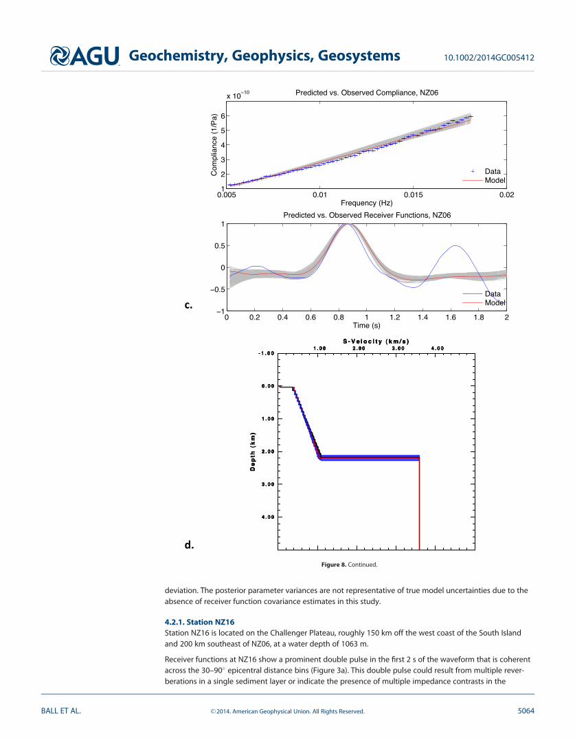
4.2. Sediment Velocity Structure from P-S Mode Conversions and Seafloor Compliance at MOANAStationsWe jointly model MOANA seafloor compliance data and receiver functions using the MC algorithm to pro-duce sediment velocity and thickness estimates for MOANA stations NZ06 and NZ16 (Figures 7 and 8). Only

Figure 7. Joint compliance and receiver function inversion results for station NZ16 (surface waves not included—see Figure 10 for inver-sion including surface waves). The model was parameterized as three constant-velocity sediment layers. (a) Observed versus predictedseafloor compliance data (top) and receiver functions (bottom). (b) Starting (black) and mean posterior shear velocity model (red). Blueand gray-shaded regions indicate models and resulting data within one standard deviation of the posterior parameter means. Complianceand receiver function inversion results for station NZ16, parameterized as two sediment layers with linear velocity gradients. (c) Observedversus predicted seafloor compliance data (top) and receiver functions (bottom). (d.) Starting (black) and mean posterior shear velocitymodel (red). Blue and gray-shaded regions indicate models and data within one standard deviation of the posterior means.



the first 2 s of the receiver function waveforms are used in the sediment study in order to isolate the firstsediment P-S conversions, which constrain only the total travel time through the sediment column. The sea-floor compliance data provide a complimentary constraint on sediment shear velocity.

To estimate sediment velocity structure, we fix crustal thickness in our model to the estimates of Grobyset al. [2008]. We then construct trial starting models with sediment thicknesses ranging between those pre-sented in the sonobuoy/refraction results of Divins [2003] (assumed to be minimum thicknesses) and thegravity modeling results of Wood and Woodward [2002].

The Monte Carlo search was performed in successive stages of 5000 iterations with a burn-in period of 1000iterations to allow Markov chain stabilization. Between stages, the misfit parameters were adjusted to

Figure 7. Continued.



weight receiver functions and seafloor compliance equally, and the starting model for the next stage wasconstructed using the posterior parameter Markov chain means from the previous stage. The resultingvelocity models and data fits are presented here as the means of the parameter Markov chains 61 standard

Figure 8. Compliance and receiver function inversion results for station NZ06, parameterized as three constant-velocity layers. (a) Observedversus predicted seafloor compliance data (top) and receiver functions (bottom). (b) Starting (black) and mean posterior shear velocity model(red). Blue and gray-shaded regions indicate models and data within one standard deviation of the posterior mean. Compliance and receiverfunction inversion results for station NZ06, parameterized as two sediment layers with linear velocity gradients. (c) Observed versus predictedseafloor compliance data (top) and receiver functions (bottom). (d) Starting (black) and mean posterior shear velocity model (red). Blue-shaded and gray-shaded regions indicate models and data within one standard deviation of the posterior mean.



deviation. The posterior parameter variances are not representative of true model uncertainties due to theabsence of receiver function covariance estimates in this study.

4.2.1. Station NZ16Station NZ16 is located on the Challenger Plateau, roughly 150 km off the west coast of the South Islandand 200 km southeast of NZ06, at a water depth of 1063 m.

Receiver functions at NZ16 show a prominent double pulse in the first 2 s of the waveform that is coherentacross the 30–90� epicentral distance bins (Figure 3a). This double pulse could result from multiple rever-berations in a single sediment layer or indicate the presence of multiple impedance contrasts in the

Figure 8. Continued.



sediment column. When searching over a model space of three constant-velocity layers, the Monte Carloanalysis of seafloor compliance and receiver functions predicts a total sediment thickness of 1.4 km butunderpredicts the amplitude of the first receiver function pulse (Figure 7a). When linear velocity gradientsare employed in the model, the receiver function fit improves markedly and the estimated sediment thick-ness decreases to only 800 m (Figures 7c and 7d).

4.2.2. Station NZ06Station NZ06 is located � 350 km off the west coast of the South Island of New Zealand on the Chal-lenger Plateau in 859 m of water. Receiver functions at NZ06 show high-amplitude sediment reverbera-tions and the waveforms are more weakly correlated across epicentral distance bins than those fromNZ16 (Figure 3).

Monte Carlo results for the three-layered model at NZ06 estimate a total sediment thickness of 1.7 km, andindicate a shallow impedance contrast at 35m but fit the compliance curve poorly (Figure 8a). The linear-gradient model yields a total sediment thickness estimate of 2.2 km, exhibits no shallower discontinuitiesand does not fit the second pulse in the receiver function (Figures 8c and 8d).

4.3. Crustal Thickness and Shear Velocity Structure From Monte Carlo Modeling of SeafloorCompliance, Receiver Functions, and Rayleigh DispersionTo investigate the feasibility of this technique in resolving deeper features such as the Moho, we added Ray-leigh dispersion to the input data and extended the modeled receiver function waveforms to include arriv-als originating from deeper structure. We use the means of the posterior model parameter distributionsfrom the sediment analysis in subsection 4.2 combined with average crustal shear velocities from thesurface-wave inversion in subsection 2.2.1 to form starting models for the crustal-scale analysis (Figure 9).Starting Moho depths were estimated using Grobys et al. [2008]. Misfit in the predicted versus observedreceiver functions is calculated to 6 s in the waveform to include Moho P-S conversions and reverberations.Predicted versus observed phase velocity dispersion is added to the misfit functional and the algorithm isrun in the same manner as discussed in subsection 4.2 above. Due to low SNR in the MOANA receiver func-tions, the full crustal-scale combined receiver function, surface wave, and compliance analysis is limited tostation NZ16.

A total crustal thickness of 22 km is obtained from joint inversion of RFs, compliance, and surface wave dataat NZ16 (Figure 9). However, in the starting model, a Moho depth of 22 km was used based on the modelsof Grobys et al. [2008], and the Monte Carlo accepted no model realizations that deviated substantially fromthis value, as shown by the posterior crustal thickness standard deviation plotted in blue shading in Figure9b. Our synthetic test showed similar behavior at receiver function SNR below 10 (Figure 6) illustrating thatreceiver function data sensitivity is poor at longer times in the waveform due to noise, and that a local mini-mum in the cost function around the starting crustal thickness could result from using noisy receiver func-tions in this method. The shallow sediment parameters were left free in the deeper inversion and asediment layer thickness of 800 m was estimated, falling near the values of 711 m and 800 m produced bythe constant-velocity and linear gradient sediment-scale analysis (Figure 7).

5. Discussion

At station NZ16 the estimated sediment thickness of 800 m from the gradient model agrees generally withthe 711 m acoustic basement depth reported by Divins [2003]. Sediment thickness estimates from both thethree layer and gradient models fall within the 2.0 6 1.5km thickness estimate from gravity modeling byWood and Woodward [2002], but the gradient model yields lower joint misfit at this station. We also observeshear resonances in horizontal-component ambient noise data at NZ16 that are potentially related to thepresence of shear velocity gradients in the shallow sediments there [Godin and Chapman, 1999].

When the surface wave data are modeled in conjunction with receiver functions at NZ16, we estimate acrustal thickness of 22 km, which does not deviate from the 22 km starting Moho depth we assume fromGrobys et al. [2008]. The implausibly low standard deviation of the posterior crustal thickness illustrates thatthe joint misfit is not being substantially reduced by varying this parameter in the Monte Carlo search. Thisbehavior was also seen in our synthetic testing (Figure 6). According to our synthetic tests, a receiver func-tion SNR on the order of 10 is likely necessary to constrain crustal thickness with this method. This is



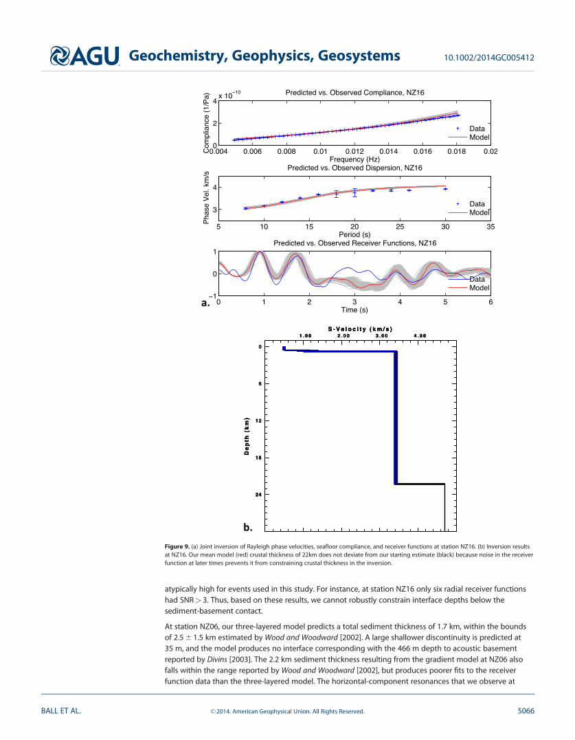
atypically high for events used in this study. For instance, at station NZ16 only six radial receiver functionshad SNR> 3. Thus, based on these results, we cannot robustly constrain interface depths below thesediment-basement contact.

At station NZ06, our three-layered model predicts a total sediment thickness of 1.7 km, within the boundsof 2.5 6 1.5 km estimated by Wood and Woodward [2002]. A large shallower discontinuity is predicted at35 m, and the model produces no interface corresponding with the 466 m depth to acoustic basementreported by Divins [2003]. The 2.2 km sediment thickness resulting from the gradient model at NZ06 alsofalls within the range reported by Wood and Woodward [2002], but produces poorer fits to the receiverfunction data than the three-layered model. The horizontal-component resonances that we observe at

Figure 9. (a) Joint inversion of Rayleigh phase velocities, seafloor compliance, and receiver functions at station NZ16. (b) Inversion resultsat NZ16. Our mean model (red) crustal thickness of 22km does not deviate from our starting estimate (black) because noise in the receiverfunction at later times prevents it from constraining crustal thickness in the inversion.



NZ16 and associate with the presence of shallow sediment shear velocity gradients are not prominentlyseen on NZ06 noise data.

It is evident from these results that the choice of model parameterization has a crucial influence on sedi-ment models resulting from the inversion of seafloor compliance and receiver function data. Based on jointdata misfit, the linear-gradient model is more appropriate for NZ16, while the layer-cake model is preferredat NZ06. Our observations of sediment shear modes also support the presence of large shallow velocity gra-dients at NZ16 but not at NZ06.

Seafloor compliance probes bulk shear velocities while receiver functions are sensitive to impedance con-trasts across interfaces. We find that the simple parameterizations investigated here are not always suffi-cient to jointly model features demanded by these separate datasets. For example, the compliance data forNZ06 are best fit by a linear velocity gradient, but this parameterization does not result in a model with thedual impedance contrasts required to fit both receiver function pulses. A nonlinear velocity gradient para-meterized using a power law [Godin and Chapman, 1999] or spline [Shen et al., 2013] formulation may pro-vide an improved fit to the slope of the compliance curve while allowing for the large impedance contrastsnecessary to fit the receiver function data.

The evident trade-off in data sensitivity between compliance and receiver functions also motivates the useof a transdimensional inversion scheme for these data, in which the model parameterization itself is treatedas an unknown [Bodin et al., 2012]. In addition, data noise can be treated as a free parameter in a trans-dimensional Monte Carlo search. In such case, the posterior distributions would reflect meaningful modeluncertainties, rather than simply depending on ad hoc cost-function weighting parameters as they do inthis study.

Our receiver function data did not conclusively resolve crustal structure beneath the sediment layer withthis method. However, an alternate technique to mitigate the overprinting effects of sediments in OBSreceiver functions is redatuming to virtual receivers below the sediments, as successfully applied on landdata from the Mississippi Embayment by Langston [2011]. The success of redatuming relies critically uponaccurate a priori knowledge of sediment thickness and velocity structure. Promisingly, the method we pres-ent here can be used to estimate these parameters using P-S converted arrival times and seafloor compli-ance data to, respectively, constrain sediment thickness and shear velocity, opening up a potential researchavenue for improving the utility of OBS receiver functions in the future.

6. Conclusions

We introduce a new method to combine seafloor compliance, receiver functions, and Rayleigh wave disper-sion in order to determine suboceanic crustal properties. We utilize a Markov Chain Monte Carlo approachto sample the model space and produce probabilistic estimates of shear velocity structure. We use themethod to first determine shallow sediment properties, which are then used as an a priori estimate in ourmodeling of the deeper crust. Well-determined sediment properties are essential for modeling the sedi-ment layer reverberations that can dominate OBS receiver functions. Our tests with synthetic data are prom-ising. However, tests with real data are mixed. We have good success in determining shallow sedimentproperties from the combination of seafloor compliance and receiver functions, and good success in deter-mining crustal shear wave velocity from the combination of seafloor compliance and Rayleigh wave disper-sion. Our results with synthetic and real data indicate that resolution of the Moho interface from OBSreceiver functions remains elusive, even in combination with a well-determined sedimentary layer. Reda-tuming methods may hold more promise, and will rely on a well-determined sedimentary layer, as providedhere. Our success in determining shallow interface properties suggests that our method may be of use forapplication to other shallow targets, such as magma chambers or hydrocarbon reservoirs.

ReferencesBodin, T., M. Sambridge, H. Tkalcic, P. Arroucau, K. Gallagher, and N. Rawlinson (2012), Transdimensional inversion of receiver functions

and surface wave dispersion, J. Geophys. Res., 117, B02301, doi:10.1029/2011JB008560.Bostock, M. G., and A. M. Trehu (2012), Wave-field decomposition of ocean bottom seismograms, Bull. Seismol. Soc. Am., 102, 1681–1692.Castagna, J. P., M. L. Batzle, and R. L. Eastwood (1985), Relationships between compressional-wave and shear-wave velocities in clastic sili-

cate rocks, Geophysics, 50(4), 571–581.

AcknowledgmentsThe data used here are publiclyavailable from the IncorporatedResearch Institutions for Seismologyunder network code ZU, years 2009–2010. We thank the Ocean-BottomSeismograph group at ScrippsInstitution of Oceanography forproviding and operating the OBS. Thisresearch was supported by theNational Science Foundation undergrants EAR-0409835 and EAR-0409609.J.C.S. was supported by a CIRES visitingfellowship at the University ofColorado and A.F.S. was supported bya visiting professorship at theEarthquake Research Institute,University of Tokyo, for a portion ofthis work. The authors thank RobertHerrmann for his modifications to theCPS330 software package and SpahrWebb, Oleg Godin, Weisen Shen,Julien Chaput, Stan Dosso, ThomasBodin, James Gaherty and ananonymous reviewer for theirthoughtful comments and discussion.



http://dx.doi.org/10.1029/2011JB008560

Collins, J. A., and P. Molnar (2014), Pn anisotropy beneath the South Island of New Zealand and implications for distributed deformation incontinental lithosphere, J. Geophys. Res. Solid Earth, 119, doi:10.1002/2014JB011233.

Crawford, W., S. C. Webb, and J. Hildebrand (1991), Seafloor compliance observed by long-period pressure and displacement measure-ments, J. Geophys. Res., 96(10), 16,151–16,160.

Divins, D. L. (2003), Total Sediment Thickness of the World’s Oceans & Marginal Seas, NOAA Natl. Geophys. Data Cent., Boulder, Colo.Filloux, J. H. (1983), Pressure fluctuations on the open ocean floor off the Gulf of California: Tides, Earthquakes, Tsunamis, J. Phys. Oceanogr.,

13, 783–786.Forsyth, D. W., S. C. Webb, L. M. Dorman, and Y. Shen (1998), Phase velocities of Rayleigh waves in the MELT experiment on the East Pacific

Rise, Science, 280, 1235–1238, doi:10.1126/science.280.5367.1235.Godin, O. A., and D. M. F. Chapman (1999), Shear-speed gradients and ocean seismo-acoustic noise resonances, J. Acoust. Soc. Am., 106(5),

2367–2381.Grobys, J. W. G., K. Gohl, and G. Eagles (2008), Quantitative tectonic reconstructions of Zealandia based on crustal thickness estimates, Geo-

chem. Geophys. Geosyst., 9, Q01005, doi:10.1029/2007GC001691.Haario, H., M. Laine, A. Mira, and E. Saksman (2006), DRAM: Efficient adaptive MCMC, Stat. Comput., 16, 339–354, doi:10.1007/s11222-006-

9438-0.Harmon, N., D. W. Forsyth, R. Lamm, and S. C. Webb (2007), P and S wave delays beneath intraplate volcanic ridges and gravity lineations

near the East Pacific Rise, J. Geophys. Res., 112, B03309, doi:10.1029/2006JB004392.Herrmann, R. B. (2013), Computer programs in seismology: An evolving tool for instruction and research, Seismo. Res. Lett., 84, 1081–1088,

doi:10.1785/0220110096.Herrmann, R. B., and C. J. Ammon (2004), Surface waves, receiver functions and crustal structure, in Computer Programs in Seismology, ver-

sion 3.30, St. Louis Univ., Saint Louis, Mo.Het�enyi, G., R. Cattin, J. Vergne, and J. L. N�ab�elek (2006), The effective elastic thickness of the India plate from receiver function imaging,

gravity anomalies and thermomechanical modeling, Geophys. J. Int., 167(3), 1106–1118.Kennett, J. P., et al. (1975), Site 284, in Initial Reports of the Deep Sea Drilling Project, vol. 29, edited by J. P. Kennett et al., pp. 403–445,

U.S. Gov. Print. Off., Washington, D. C., doi:10.2973/dsdp.proc.29.111.1975.Lagarias, J. C., J. A. Reeds, M. H. Wright, and P. E. Wright (1998), Convergence properties of the Nelder-Mead simplex method in low dimen-

sions, SIAM J. Optim., 9(1), 112–147.Langston, C. (1979), Structure under Mount Rainier, Washington, inferred from teleseismic body waves, J. Geophys. Res., 84(B9), 4749–4762.Langston, C. (2011), Wave-field continuation and decomposition for passive seismic imaging under deep unconsolidated sediments, Bull.

Seismol. Soc. Am., 101(5), 2176–2190.Leahy, G. M., J. A. Collins, C. J. Wolfe, G. Laske, and S. C. Solomon (2010), Underplating of the Hawaiian swell: Evidence from teleseismic

receiver functions, Geophys. J. Int., 183(1), 313–329.Ligorria, J., and C. Ammon (1999), Iterative deconvolution and receiver-function estimation, Bull. Seismol. Soc. Am., 89(5), 1395–1400.Lin, F.-C., M. H. Ritzwoller, J. Townend, S. Bannister, and M. K. Savage (2007), Ambient noise Rayleigh wave tomography of New Zealand,

Geophys. J. Int., 170(2), 649–666.Lin, F.-C., M. P. Moschetti, and M. H. Ritzwoller (2008), Surface wave tomography of the western United States from ambient seismic noise:

Rayleigh and Love wave phase velocity maps, Geophys. J. Int., 173, 281–298, doi:10.1111/j.1365-246X.2008.03720.x.Lin, F.-C., M. H. Ritzwoller, and R. Snieder (2009), Eikonal Tomography: Surface wave tomography by phase-front tracking across a regional

broad-band seismic array, Geophys. J. Int., 177, 1091–1110, doi:10.1111/j.1365-246X.2009.04105.x.Mosegaard, K., and A. Tarantola (1995), Monte Carlo sampling of solutions to inverse problems, J. Geophys. Res., 100(B7), 12,431–12,447.Owens, T. J., G. Zandt, and S. R. Taylor (1988), Seismic evidence for an ancient rift beneath the Cumberland Plateau, Tennessee: A detailed

analysis of broadband teleseismic P waveforms, Bull. Seismol. Soc. Am., 78, 96–108.Park, J., and V. Levin (2000), Receiver functions from multiple-taper spectral correlation estimates, Bull. Seismol. Soc. Am., 90(6), 1507–1520.Ritzwoller, M. H., and A. L. Levshin (2002), Estimating shallow shear velocities with marine multicomponent seismic data, Geophysics, 67(6),

1991–2004.Scherwath, M., T. Stern, F. Davey, D. Okaya, W. S. Holbrook, R. Davies, and S. Kleffmann (2003), Lithospheric structure across oblique conti-

nental collision in New Zealand from wide-angle P wave modeling, J. Geophys. Res., 108(B12), 2566, doi:10.1029/2002JB002286.Shen, W., M. H. Ritzwoller, V. Schulte-Pelkum, and F.-C. Lin (2013), Joint inversion of surface wave dispersion and receiver functions: A

Bayesian Monte-Carlo approach, Geophys. J. Int., 192, 807–836, doi:10.1093/gji/ggs050.Stachnik, J. C., K. Dueker, D. L. Schutt, and H. Yuan (2008), Imaging Yellowstone plume-lithosphere interactions from inversion of ballistic

and diffusive Rayleigh wave dispersion and crustal thickness data, Geochem. Geophys. Geosyst., 9, Q06004, doi:10.1029/2008GC001992.Stern, T., D. Okaya, and M. Scherwath (2002), Structure and strength of a continental transform from onshore-offshore seismic profiling of

South Island, New Zealand, Earth Planet. Space, 54(11), 1011–1020.Thorwart, M., and T. Dahm (2005), Wavefield decomposition for passive ocean bottom seismological data, Geophys. J. Int., 163(2), 611–621.Van Avendonk, H., J. A., W. S. Holbrook, D. Okaya, J. K. Austin, F. Davey, and T. Stern (2004), Continental crust under compression: A seismic

refraction study of South Island Geophysical Transect I, South Island, New Zealand, J. Geophys. Res., 109, B06302, doi:10.1029/2003JB002790.

Webb, S. C. (1998), Broadband seismology and noise under the ocean, Rev. Geophys., 36(1), 105–142.Willoughby, E., and R. Edwards (2000), Shear velocities in Cascadia from seafloor compliance, Geophys. Res. Lett., 27(7), 1021–1024.Wood, R., and D. Woodward (2002), Sediment thickness and crustal structure of offshore Western New Zealand from 3d gravity modeling,

N. Z. J. Geol. Geophys., 45(2), 243–255.Yang, Z., A. F. Sheehan, J. A. Collins, and G. Laske (2012), The character of seafloor ambient noise recorded offshore New Zealand: Results

from the MOANA ocean bottom seismic experiment, Geochem. Geophys. Geosyst., 13, Q10011, doi:10.1029/2012GC004201.Ye, T., W. Shen, and M. H. Ritzwoller (2013), Crustal and uppermost mantle shear velocity structure adjacent to the Juan de Fuca Ridge

from ambient seismic noise, Geochem. Geophys. Geosyst., 14, 3221–3233, doi:10.1002/ggge.20206.Zietlow, D. W., A. F. Sheehan, P. H. Molnar, M. K. Savage, G. Hirth, J. A. Collins, and B. H. Hager (2014), Upper mantle seismic anisotropy at a

strike slip boundary: South Island, New Zealand, J. Geophys. Res. Solid Earth, 119, 1020–1040, doi:10.1002/2013JB010676.



http://dx.doi.org/10.1002/2014JB011233

http://dx.doi.org/10.1126/science.280.5367.1235

http://dx.doi.org/10.1029/2007GC001691

http://dx.doi.org/10.1007/s11222-006-9438-0

http://dx.doi.org/10.1007/s11222-006-9438-0

http://dx.doi.org/10.1029/2006JB004392

http://dx.doi.org/10.1785/0220110096

http://dx.doi.org/10.2973/dsdp.proc.29.111.1975

http://dx.doi.org/10.1111/j.1365-246X.2008.03720.x

http://dx.doi.org/10.1111/j.1365-246X.2009.04105.x

http://dx.doi.org/10.1029/2002JB002286

http://dx.doi.org/10.1093/gji/ggs050

http://dx.doi.org/10.1029/2008GC001992

http://dx.doi.org/10.1029/2003JB002790

http://dx.doi.org/10.1029/2003JB002790

http://dx.doi.org/10.1029/2012GC004201

http://dx.doi.org/10.1002/ggge.20206

http://dx.doi.org/10.1002/2013JB010676

a joint monte carlo analysis of seafloor compliance ...noise.earth.utah.edu/ggge20616.pdf · ously...

Documents