a kink that makes you sick: the effect of sick pay on absence in a social insurance system

292A Kink that Makes You Sick:The Incentive Effect of Sick Pay on Absence

Petri Böckerman*Ohto Kanninen**Ilpo Suoniemi***

297A Kink that Makes You Sick: the Effect of Sick Pay on Absence in a Social Insurance System

Petri BöckermanOhto KanninenIlpo Suoniemi

Helsinki 2015

* We would like to thank the Social Insurance Institution of Finland (KELA) for financial support and access to their data. We aregrateful to Mark Borgschulte, Ulla Hämäläinen, Olli Kangas, Benjamin Marx, Tuomas Matikka, Jukka Pirttilä and Marko Terviö for

discussions. We also thank participants at the EEA and EALE annual meetings as well as HECER, KELA, Government Institute for Economic Research, the Labour Institute for Economic Research and University of Illinois microeconomics seminars for comments.

We are also grateful to Zhuan Pei for his help with the method. The data used in this study are confidential but other researchers can independently obtain access to it for replication purposes by the permission from the Social Insurance Institution of Finland. To obtain access to the data, please contact the Social Insurance Institution of Finland, P.O. Box 450 FI-00101, Helsinki, Finland. The specific instructions to obtain access to the data are available at http://www.kela.fi/web/en/research-projects_research-data-requests. The computer programs to generate the results of the study for replication purposes are available from Ohto Kanninen.

The data that we use do not have Institutional Review Board (IRB) Approval. We use administrative register data. The study does not disclose information concerning individual persons. The data have been constructed for research purposes in the Social

Insurance Institution of Finland, under the ethical guidelines of the institution which comply to the national standards.

The authors declare that they have no relevant or material financial interests that relate to the research described in this paper.

** Turku School of Economics, Labour Institute for Economic Research and IZA. Address: Pitkänsillanranta 3A, FI-00530 Helsinki, Finland. Phone: +358-9-2535 7330. Fax: +358-9-2535 7332. E-mail: [email protected]

*** Labour Institute for Economic Research. E-mail: [email protected]

**** Labour Institute for Economic Research. E-mail: [email protected]

TYÖPAPEREITA 297WORKING PAPERS 297

Palkansaajien tutkimuslaitosPitkänsillanranta 3 A, 00530 HelsinkiPuh. 09−2535 7330Sähköposti: [email protected]

Labour Institute for Economic ResearchPitkänsillanranta 3 A, FI-00530 Helsinki, FinlandTelephone +358 9 2535 7330E-mail: [email protected]

ISBN 978–952–209–137–6 (pdf)ISSN 1795–1801 (pdf)

Tiivistelmä

Tutkimuksessa arvioidaan Kelan maksaman sairauspäivärahan vaikutusta sairauspoissa-

olojen kestoon. Sairauspäivärahan vaikutuksen estimointi perustuu ns. kulmapistemene-

telmään, sillä päivärahan määräytymissäännön kulmakertoimessa on hyppäyksiä

kiinteillä tulotasoilla. Kulmapistemenetelmällä kvasikokeellinen kausaalivaikutus

vastemuuttujaan voidaan identifioida, jos tarkastelun kohteena oleva politiikkamuuttuja

on tunnettu, deterministinen ja kulmapisteellinen funktio sitä määräävästä muuttujasta.

Tässä sovelluksessa politiikkamuuttuja on sairauspäivärahan laskukaava, määrittelevä

muuttuja on kahden vuoden takaiset tulot ja vastemuuttuja on sairauspoissaolojakson

kesto. Tutkimuksessa havaitaan, että korkeampi korvaustaso pidentää selvästi sairaus-

poissaolojaksoja. Poissaolojaksojen keston jousto korvaussuhteen suhteen on noin 1.

Tulosten avulla luonnehditaan optimaalista sairausvakuutusjärjestelmää, sillä sosiaali-

vakuutuksen optimaalinen korvaustaso määräytyy joustoparametrin ja riskinkarttamis-

parametrien kautta.

Abstract

We examine the effect of the replacement rate of a social insurance system on sickness

absence by exploiting a regression kink design. The elasticity of absence with respect to

the benefit level, in addition to risk preferences, is a critical parameter in defining the

optimal sickness insurance scheme. Using a large administrative dataset, we find a robust

behavioral response. The statistically significant point estimate of the elasticity of the

duration of sickness absence with respect to the replacement rate in a social insurance

system is on the order of 1. Given our estimate, we characterize the optimal benefit level.

Keywords: Sick pay, labor supply, sickness absence, regression kink design, social

insurance

JEL classification: H55, I13, J22

2

1. Introduction

Absenteeism causes a substantial loss of working time worldwide. In some OECD

countries nearly 10% of annual working days are lost because of sickness absence (DICE

Database, 2012).1 The costs are considerable for the individual, employers, co-workers,

and health and benefit systems. Sickness absence is also a source of major indirect costs,

because it increases the risk of withdrawing from the labor force (e.g. Kivimäki et al.

2004).

A sickness insurance system protects individuals from earnings losses. Among cash

benefits, sickness insurance is one of the most important social protection schemes in

Europe (Eurostat, 2011). The key policy parameter is the replacement rate, i.e. the ratio

of sickness insurance benefits to past earnings.

We examine the effect of the replacement rate of the Finnish sickness insurance on the

duration of sickness absence. We find a substantial and robust behavioral effect. The

statistically significant point estimate of the elasticity of the duration of sickness absence

with respect to the replacement rate is 0.83 or 1.41, depending on the model

specification.

The elasticity of the duration of sickness absence is a relevant parameter of an optimal

sickness insurance system (Baily, 1978; Chetty, 2006). The replacement rate directly

affects workers’ financial incentives to be absent from work at the intensive margin of

labor supply through a moral hazard effect.

We use Regression Kink Design (RKD, see Section 4) to identify the causal effect of the

replacement rate. Unlike in most other countries (Frick and Malo, 2008, p. 510-511), the

compensation level of sickness insurance in Finland is not a fixed fraction of past

earnings, but it follows a piecewise linear scheme. This allows us to use RKD, in which

the identification of the effect is based on a pre-determined, nonlinear policy rule

(Nielsen et al. 2010; Card et al. 2012).2

1 Treble and Barmby (2011) provide an overview.

2 See Table 1 in Ganong and Jäger (2014) for a list of RKD applications.

3

Previous research has used policy reforms that provide exogenous variation in the

replacement rates to examine the effect of sick pay level on absence. Several studies

exploit legislative changes in the replacement rates and provide difference-in-difference

estimates for Sweden (Henrekson and Persson, 2004; Johansson and Palme, 2005;

Pettersson-Lidbom and Skogman Thoursie, 2013). There is also similar evidence for

other countries (Puhani and Sonderhof, 2010; De Paola et al. 2014; Ziebarth and

Karlsson, 2014; Fevang et al. 2014). Most other countries, including the U.S., have more

fragmented sickness insurance schemes which complicate the analysis (cf. Gruber, 2000).

In addition to studies that have exploited policy reforms within countries, there is cross-

country evidence on the positive effect of the replacement rate of sickness insurance on

absenteeism (Frick and Malo, 2008).

The elasticity of absence with respect to the replacement rate is positive, based on earlier

research. However, the quantitative size of the effect varies substantially from study to

study. Also, the comparison of the estimates is not straightforward, since the outcome

variables (duration of sickness absence or number of sickness absence days) are not

identical in all studies.

Empirical studies based on policy reforms suffer from a number of caveats. Reforms are

aimed at specific groups, the causal impact takes time to take effect, agents anticipate the

upcoming reform,3 effects are confounded by simultaneous policy changes or other

shocks, and long-term wealth effects are challenging to identify. Thus, the causal

interpretation for the difference-in-difference estimates based on policy reforms is not

straightforward (cf. Besley and Case, 2000; Pettersson-Lidbom and Skogman Thoursie,

2013, p. 487).

We improve upon previous literature by using a method that allows us to focus on all

employees around the kink point in the benefit rule. The kink point provides policy-

relevant exogenous variation in the neighborhood of the median income. A long-standing

quasi-experiment is likely to reveal equilibrium behavior. We interpret our estimate as

the Frisch elasticity. We recast the search models by Baily (1978) and Chetty (2006) of

3 De Paola et al. (2014, p. 349) highlight the fact that employees can adjust their sickness absence behavior

in anticipation of the reform.

4

optimal unemployment insurance to interpret our results. The models compare universal

sickness insurance to self-insurance.

The paper unfolds as follows. Section 2 discusses the theoretical aspects of an optimal

mandatory sickness insurance system. Section 3 provides an overview of the Finnish

sickness insurance system. Section 4 describes RKD. Section 5 introduces the data and

the estimation results are presented in Section 6. The last section concludes.

2. Optimal sickness insurance system

In the absence of private insurance, social planner faces a trade-off: an optimal social

insurance system balances the costs of more generous payments to the sick with the

welfare gain resulting from the consumption smoothing that the benefits allow (Baily,

1978; Chetty, 2006; Chetty and Saez, 2010). A critical input in defining the optimal

replacement rate in a mandatory sickness insurance program is the elasticity of absence

w.r.t. the generosity of benefits. The elasticity captures the relevant costs of a higher

benefit level.

The search model of optimal unemployment insurance benefit compares unemployment

insurance scheme which is financed by a budget-balancing tax while working to self-

insurance using prior assets as a buffer-stock.4 The unobserved cost of effort of an early

return to work induces moral hazard to the model.5

In comparative statics it is important to separate effects that refer to shifts in a life-cycle

wage profile (wealth effects) and movements along a given wage profile. The labor

supply response to wage changes is generally a mixture of an intertemporal substitution

effects, compensated wage elasticity and wealth effects. The intertemporal (i.e. Frisch)

elasticities hold the marginal utility of wealth constant and compensated elasticities hold

lifetime utility constant. Intertemporal responses are greater than compensated responses

4 A mandatory insurance system prevents adverse selection out of insurance coverage. However, in the

presence of heterogeneity, some workers have more to gain from insurance than others. We leave any

heterogeneity effects out of the analysis. 5 The unobserved cost of job search in the unemployment insurance model is reinterpreted in our setting as

the cost of effort to an early return to work while on sick leave.

5

and they reduce to the same value only if income or wealth effects are zero (Macurdy,

1981, pp. 1070-1073).

The MaCurdy (1981) critique maintains that studying a reform which changes the whole

net-of-tax wage profile does not recover the Frisch elasticity, since the reforms affect

wealth. In our setting, workers return to work with the same wage level as before the

sickness leave. In addition, the wealth effect on life-cycle labor supply is likely to be

smaller in sickness insurance, since the spells of sickness leave (in our data the mean

spell is 44 days) are considerably shorter than typical unemployment durations (over 15

weeks). Therefore, we ignore the wealth effects6 and base the interpretation of the

estimates on the simplified two-period search models by Baily (1978, pp. 383-390) and

Chetty (2006, pp. 1882-1886).

The optimal benefit level of a social insurance system equates the marginal cost of

financing the benefit to the marginal welfare gain from consumption while on sick leave.

Using a second-order Taylor approximation, the optimality condition can be written as

(Chetty, 2006, p. 1883):

�� = �′(��) − �′(��)�′(��) ≈ ∆�� 1 +12� ∆��,

(1)

where subscript w stands for being at work, D signifies the duration of sickness leave ,

∆�/�� is the proportional drop in consumption while on sick leave, = − ��(��)��(��) is the

coefficient of relative risk aversion, � = − ��(��)��(��) is the coefficient of relative prudence

and �� = � ��(�)� ��(�) is the elasticity of the duration of sick leave with respect to the sickness

benefit.

In the absence of a private sickness insurance market and lifetime wealth effects, agents’

optimization allows us to assume that sickness benefits are spent solely on consumption

while sick and that higher taxes are financed solely by reducing consumption while at

work when computing welfare changes. The welfare change can be written in terms of

6 This assumption predicts that post sickness leave consumption is, in a stationary environment, equal to

that before sickness leave.

6

marginal utilities of consumption in the two states, eliminating all other behavioral

responses when setting the optimal benefit level except for the elasticity parameter (��) that enters the government budget constraint directly.

The reduced-form formula is quite robust (e.g. search costs and the value of leisure show

up in the optimized level of consumption while sick) and the optimality condition

captures a basic intuition that carries over to the general case (see Chetty, 2006). We

exploit a kink in the policy rule to estimate the elasticity.

3. The Finnish sickness insurance system

Finland has a universal mandatory sickness insurance scheme that covers all (16-67 years

old) permanent residents.7 The scheme guarantees compensation for the loss of earnings

owing to sickness and illness. Sickness allowances and reimbursements are defined in the

Health Insurance Act and Decree. Sickness insurance is financed by both employers and

employees. Insurance contributions are proportional to income and unrelated to the

benefit rule. The state participates by financing the minimum allowance that is paid to

those with no earnings.8

The Social Insurance Institution of Finland (KELA) pays out a Sickness Allowance (SA)

as compensation for the loss of earnings caused by an illness or injury. The SA includes

two provisions: a minimum sickness benefit and an earnings-related benefit. The

earnings-related benefit is relevant for most of employed and self-employed persons.

Before receiving the SA from KELA, the person must complete a waiting period. It

includes the day of onset of work incapacity and the following nine working days.9 The

incapacity for work must be certified by a doctor. The employee is entitled to normal

7 The description of the system is based mainly on Toivonen (2012). Kangas et al. (2013) provide a

historical account. 8 Finland has the highest share of sickness absenteeism in Europe (Gimeno et al. 2004). Sickness absence

has also increased significantly during the past 15 years. The average number of sickness absence days per

wage and salary earner was 10 in 2008, according to the Quality of Work Life Survey (Lehto and Sutela,

2009). 9 The waiting period includes Saturdays, but not Sundays or public holidays.

7

salary during the nine-day waiting period if the employment relationship has lasted at

least a month.10

After the nine-day waiting period the employee is eligible to receive an earnings-related

SA from KELA. The maximum period for SA is 300 working days (i.e. approximately a

full calendar year). All SA days within the last two years are counted towards this sum.

After the maximum has been reached, there is an assessment of eligibility for a disability

pension. The person is eligible to receive the SA again only after having worked for at

least a year.

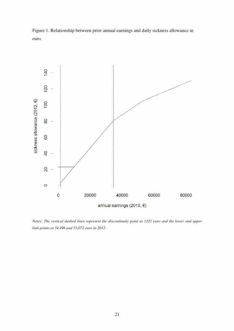
The earnings-related SA has no ceiling. This feature distinguishes the Finnish scheme

from those of the other Nordic countries and most other European sickness insurance

systems. In 2012, for annual earnings of up to 34,496 euro, the replacement rate was 70%

after which it decreased to 45% and at 53,072 euro to 30%.

For our purposes, the most important feature of the system is that the replacement rate of

the earnings-related SA follows a pre-determined, nonlinear policy rule. First, the SA is

determined by past taxable annual earnings. The relevant earnings are those earned two

calendar years before the claim for sickness insurance is made. For example, in 2012, the

SA was calculated on the basis of taxable earnings in 2010.11

Work-related expenses are

deducted from taxable earnings, and in addition a deduction is made to account for

pension and unemployment insurance contributions.

The fact that the SA is determined by past earnings is particularly useful for our

purposes, because applicants are arguably able to manipulate their current earnings. This

would invalidate the identification of the causal effect using RKD. But this is highly

unlikely regarding past earnings. Reassuringly, we are also able to check whether there is

any bunching of the data points towards the kinks in the benefit rule (see Section 6.2).

10

The employer pays a full salary for at least the first nine days, depending on the collective labor

agreement, if the employment has lasted at least a month. If the employment has lasted less than a month,

the beneficiary receives 50% of the salary. KELA fully compensates employers for these payments. 11

The amount of taxable earnings is based on the decision by the Finnish Tax Administration. An index is

used to account for the rise in wage and salary earners’ earnings (80 percent weight) and the cost of living

index (20 percent weight).

8

The second important feature of the system is that the replacement level follows a

piecewise linear policy rule in past earnings.12

The determination of SA for 2012 is

illustrated in Figure 1. There are four earnings brackets. The benefit formula for the

earnings-related SA exhibits one discontinuity and two kink points, which we define as

the lower and the upper kink point. The lower kink point allows one to use RKD to

identify the causal effect of the replacement rate. The discontinuity point cannot be

exploited, since those below the threshold receive no compensation and thus are not in

our data.

Figure 1 here

4. Regression Kink Design

4.1. Identification

Nielsen et al. (2010) propose a variant of the Regression Discontinuity Design (RDD)

which they call RKD. Their method uses a kink or kinks in a policy rule to identify the

causal effect of the policy rule on the outcome variable of interest. A valid RKD setting

requires the explanatory variable (in our case, the replacement level) to be a deterministic

and known function of an assignment variable (in our case, earnings from two years

prior). The function also has to have at least one kink point. This means that the function

has segments where it is (continuous and) differentiable, but in at least one point it is

non-differentiable having unequal left and right derivatives (Condition 1).

The second condition for a valid RKD setting is that the assignment variable allocates the

observations to the left and right segments of a kink point in a manner that is as good as

random (Condition 2). Endogenous bunching of observations near kink points (i.e.

discontinuities in the derivative of the density function) or nonlinearity of covariates

would invalidate this smoothness condition (see Card et al. 2012 for these testable

predictions). Additionally, regularity conditions are needed for a valid RKD.

12

These kinks to the system were created in the early 1980s (see Kangas 2013, p. 283).

9

In our setup, Condition 1 holds, since we know exactly how earnings from two years

prior determine the replacement level. We also have data on the relevant earnings and the

replacement level. Also, as Figure 1 shows, the relationship between the assignment

variable and the policy variable for the year 2012 is continuous for earnings above 1325

euro and has kinks at 34,496 and 53,072 euro. Other years in our data reveal a similar

structure.

The random assignment of observations (Condition 2) is not directly verifiable in

empirical applications. But it is unlikely that individuals manipulate the benefit level by

altering their earnings in order to be assigned to another segment of the replacement

function two years later. We can also ascertain that other benefit rules, such as the

earnings-related unemployment benefit, do not have kinks or discontinuities at the same

points as the sickness benefit and thus they do not affect the randomness of the

assignment. Furthermore, we can test for whether the distribution of the control variables

is smooth in relation to the kink point. If we find this not to be the case, Condition 2 fails,

which invalidates the design. This procedure is very similar to what is usually done to

validate RDD (for a review, see Imbens and Lemieux, 2008).

4.2. Formal model

Let Si be sickness days in the year t, for individual i∈{1,2,…,n}, Yi is earnings in the year

t-2 and Bi is the sickness allowance, which follows the deterministic assignment function

!" = #($") with a kink at $" = %&.The parameter of interest is the change in the slope of

the conditional expectation function '(%) = �[)"|$" = %], at %& divided by the change

in the slope of the deterministic assignment function #(%) at % = %& . The general model

of interest is of the form:

)" = ,($", !", -"), where -" is an error term.

13

Card et al. (2012) show that /, the average marginal effect of #(%), is identified at

% = %& if ,($", !", -") and its derivatives with respect to $" and !" are continuous,

13

See Nielsen et al. (2010) for the model in the following additive form: )" = /!" + 0(%) + -", where0is

a fixed function.

10

,($", !", -") has a kink (Condition 1) and the density of $" is smooth (Condition 2) at %&.

Under these assumptions, �(-"|$" = %&) is a smooth function and

/ = 12'(%&) −13'(%&)12#(%&) −13#(%&) ,

(2)

where 14'(%&) = lim8→8:;<=(8)<8 , 14#(%&) = lim8→8:;

<�(8)<8 , > ∈{+,-}. / is the weighted average

of marginal effects across the population. The weight is the relative likelihood that an

individual has$" = %&, given -" (see Card et al. 2012, pp. 8–9 for a more detailed

discussion).

The numerator in equation (2) is estimated semi-parametrically as ?@ using the following

local power series expansion:

�()"|$" = %) ≈ AB +C[AD(% − %&)D + ?D1"(% − %&)D]E

DF@,

(3)

where P is the chosen polynomial order of the estimated function and 1" is the treatment

status, where 1 means treated and 0 means not treated (1"(G) = 1, HIG > 0, 1"(G) =0otherwise). The power series is a local approximation of the conditional expectation

function of )". Note that |% − %&| ≤ ℎ, where h is the bandwidth chosen for the

estimation. The denominator in equation (2) is the change of the slope of the

deterministic #(%) at the kink point.

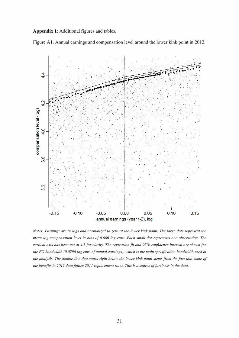
4.3. Fuzzy setting

Card et al. (2012, pp. 10–12) distinguish between sharp and fuzzy RKD. A fuzzy design

arises when there is a significant difference between the theoretical and observed value of

the kink in the policy rule. The difference stems from e.g. measurement errors or the fact

that the kink in the policy rule is affected by some unobserved and observed variables in

addition to the primary assignment variable. In our setting, a likely source of error is the

manner in which variables are defined and classified in the original dataset (see Section 5

and Figure A1).

11

In a fuzzy RKD, !"=b($", -"U). Thus, !" is now determined by unobserved factors that

might be correlated with the assignment variable. Additional assumptions are also

required for identification. Along with some technical assumptions, monotonicity in the

assignment function must hold (Condition 3). This condition states that the direction of

the kink is either non-negative or non-positive for the entire population. !" and $" are

allowed to have specific types of measurement error.

When Conditions 1, 2 and 3 and the necessary technical conditions hold,

/ = 12'(%&) −13'(%&)12#(%&) −13#(%&) ,

(4)

where 14'(%&) = lim8→8:;<=(8)<8 , 14#(%&) = lim8→8:;

<V[UW|XWF8]<8 , > ∈{+,-}./, the average

marginal effect of #(%) at % = %&, in equation (4) is weighted by the product of three

components (see Card et al. 2012, p. 12). As in a sharp RKD, the first component is the

relative probability of $" = %&. The second is the size of the kink in the benefit rule for

individual i. The third component is the probability that the assignment variable is

correctly measured at $" = %&.

For estimation of the expected change of the policy rule, we use the following local

power series expansion:

�(!"|$" = %) ≈ YB +C[YD(% − %&)D + D1"(% − %&)D]E

DF@,

where γ@ is the empirical counterpart of the policy rule. The elasticity of interest can be

approximated as / ≈ [\]\ . To obtain the correct point estimate and standard errors for τ,

we use instrumental variable (IV) regression, following Card et al. (2012, pp. 20–21).

The instrument is the interaction term of past earnings and an indicator of earnings above

the lower kink point, 1"(% − %&). The instrumented variable is !", the received

compensation.

12

4.4. Bandwidth selector

The bandwidth selection is a trade-off between bias and precision. Card et al. (2012, pp.

32–33) use the “rule-of-thumb” bandwidth selector of Fan and Gijbels (1996, equation

3.20, p. 67; henceforth FG):

ℎ = �D _ ab(0)['c (D2@)(0)]bId(0)e

@bD2f g3 @bD2f,

where p is the order of the polynomial in the main specification, ab(0) and 'c (D2@)(0) are, respectively, the estimated error variance and (p+1)th order derivative of the

regression, using a wide-bandwidth polynomial regression of equation (3),14

C1 is 2.352

for the boundary case with a uniform kernel and Id(0) is estimated from a global

polynomial fit to the histogram of earnings. Bandwidth choices which are too “large”

lead to a non-negligible bias in the estimator of the conditional expectation function. We

report the results for multiple bandwidths in the sensitivity analysis and we also use a

bandwidth selector proposed by Calonico et al. (2014; henceforth CCT). Calonico et al.

(2014) build the CCT bandwidth selector upon the FG bandwidth selector.

5. Data

We use total data on Finnish sickness absence spells over the period 2004–2012. This

comprehensive register-based data originate from KELA and they are derived from the

database that is used to pay out the SA compensations. Therefore, some measurement

error might arise from the aggregation of variables when converting the original register

for research purposes.15

The administrative data cover both wage and salary earners and

self-employed persons. The data record the start and end dates for all sickness spells and

the total amount of SA paid for each person. Annual earnings are deflated to 2012 prices

by using the consumer price index.

14

We use the data for a very wide window of 0.8 log earnings for this regression, which contains 85% of

the total sample. This is done in order to keep the polynomial order within reasonable limits. The

polynomial order is chosen to minimize Akaike Information Criterion. Also, the polynomial in this context

is allowed to be nonlinear up to the pth order. This is necessary in order for 'c (D2@)(0) to exist.

15 In particular, consecutive absence spells that start within 300 days are counted as a single spell if the

diagnosis remains the same.

13

Our data consist of absence spells that last for longer than the waiting period of nine full

working days. The distribution is right-skewed.16

Thus, longer sickness absences

contribute disproportionately to the total days lost and absence costs. The data enable us

to concentrate on those absences that are affected by the incentives of the sickness

insurance system.

The data record a person’s past taxable earnings that KELA obtains directly from the

Finnish tax authorities. KELA uses the same information to calculate the SA for

beneficiaries. The data also include useful background information such as a medical

diagnosis for the reason for sick leave, which can be used to test for validity of the RKD.

The initial diagnosis of individuals is documented according to the International

Classification of Diseases (ICD-10).17

We have also linked to the data the highest

completed education from the Register of Completed Education and Degrees, maintained

by Statistics Finland.

The estimations are restricted to those in the labor force who are eligible for sick pay and

who are between 16 and 70 years of age. The final sample used in the analysis includes

compensated absence spells which are above zero in duration and whose payment criteria

and initial diagnoses are known for employees with a single employer during their

sickness spell.18

The final sample around the lower kink point consists of 37,000–41,000

individuals, depending on the year. Descriptive statistics is reported in Table 1 (duration

of sickness absence and background characteristics for persons).19

Table 1 here

16

The skewness of the distribution is 2.5 and 2.9 for the total sample and for the window of 0.0796 log

earnings around the lower kink point, respectively. 17

ICD is the standard diagnostic tool for clinical purposes. The classification is available at:

http://www.who.int/classifications/icd/en/ 18

A part-time sickness benefit was introduced in Finland at the beginning of 2007. We exclude its

recipients from the sample. Only 0.5% of the sample has no known diagnosis. Also, 146 observations with

missing received compensation were excluded. We are able to identify entrepreneurs from 2006 onwards.

We exclude the 2.3% of the original sample that entrepreneurs represent. In total, we exclude c. 3.0% of

the original data to construct the final sample. 19

A fraction of the insured (13.6%) are compensated according to an eligibility criterion other than prior

earnings (e.g. if earnings have changed by more than 20%, the compensation can be claimed based on

more recent earnings, see Toivonen 2012). Our results are robust to their exclusion from the sample (see

Table A3).

14

Figure 2 reveals that persons with low earnings have a longer duration of sickness

absence. This pattern is consistent with the hypothesis that poor health erodes earning

capacity (cf. Aittomäki et al. 2014, p. 86), assuming that the duration of sickness absence

is a valid proxy for health.

Figure 2 here

We exploit the lower kink point to identify and estimate the effect of the replacement rule

for two reasons. First, the lower kink point is located in the part of the earnings

distribution which contains substantial mass to support the estimation of statistically

significant effects (Figure A2). The large sample size around this kink point shows as

smaller variability in the length of sickness absence within the 800 euro bins. Second,

there is a large change in the benefit rule at the lower kink point (cf. Figure 1).20

6. Results

6.1. Baseline estimates

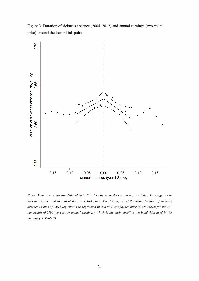
Figure 3 illustrates the duration of sickness absence and annual earnings around the lower

kink point.21

It suggests that there is a behavioral response at the kink.

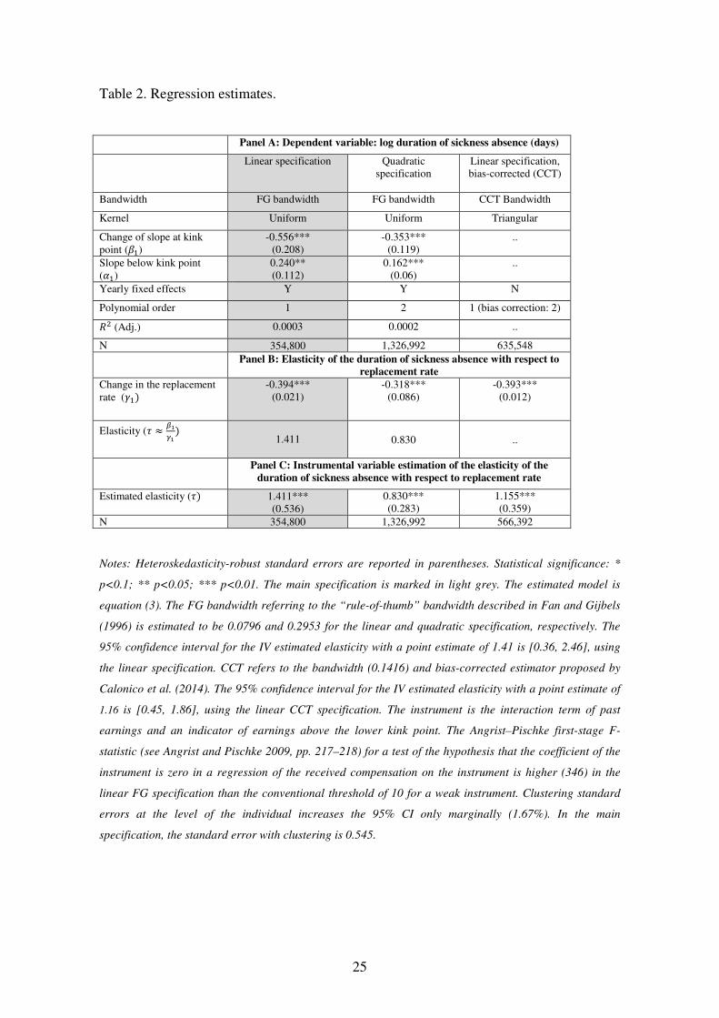
Using the FG bandwidth of 0.0796 log euro for annual earnings, we find clear evidence

for the incentive effects (see Table 2 and Table A1). The estimated change of the slope at

the lower kink point is -0.56. The weighted average of the marginal elasticities of the

duration of sickness absence (/) with respect to the replacement rate is 1.41 [95% CI:

0.36, 2.46] using the linear specification. The point estimate implies a high elasticity. The

quadratic specification (i.e. when h = 2) gives a point estimate of 0.83 [0.27, 1.38] with

the FG bandwidth of 0.2953 also implying a significant behavioral response. Using the

20

The estimated effects are insignificant at the upper kink point and thus omitted. There are multiple

reasons for the insignificance of the estimate: fewer data points, smaller slope change and potentially

heterogeneous treatment effects. The point estimate for the linear upper kink estimate is 0.426 (1.677). FG

bandwidth is 0.086. The quadratic model gives a point estimate of 0.436 (0.454). FG bandwidth is 0.463. 21

The bandwidth in Figure 3 was chosen for illustrative purposes to mitigate excessive noise, following the

methodological guidance of Lee and Lemieux (2010). The number of bins used coincides with the number

given by Sturges’ rule (Sturges, 1926), which is a classic method for choosing the optimal number of bins

for histograms. See Figure A3 for the same graph without the fit and confidence interval, but illustrating

the sample size around the kink point. Figures A4 and A5 report the annual graphs.

15

CCT22

(Calonico et al. 2014) bias-corrected estimator and bandwidth (0.1416), we

estimate the elasticity to be 1.16. The CCT was estimated using the triangular kernel.23

Figure 3 and Table 2 here

The wider the bandwidth used, the lower the point estimates get. This result is illustrated

in Figure 4. If functions �()"|$" = %) and �(!"|$" = %) are piecewise linear and the

sample size is sufficiently large, then the point estimate would remain unchanged with all

bandwidths, i.e. the relationship depicted in Figure 4 would be a horizontal line. Thus,

deviations from the horizontal line are indicative of curvature in the conditional

expectation functions and consequently the presence of bias in the local linear estimator.

Figure 4 here

The choice of bandwidth is a compromise between precision and bias. The main

specification uses the FG bandwidth h, estimated to be 0.0796 log euro, which fulfils two

criteria. First, covariates are linear, whereas they show nonlinearity at wider bandwidths

(see Table A2) than 0.0796 log euro. Second, estimates are sufficiently precise, whereas

a narrower band would increase standard errors.

Precision in regression analysis increases with sample size and variance in the

explanatory variable. Both of these decrease as the bandwidth narrows. Note that the FG

bandwidth that we use in our main specification is quite narrow in terms of monthly

earnings (~460 euro in 2012).

22

The CCT estimator is singularly compute-intensive in our setting. 23

The FG bandwidth depends on the polynomial order. Under the same bandwidth sequence, the variance

of the local quadratic estimator with a uniform kernel is 16 times as large as its local linear counterpart (see

Card et al. 2012, pp. 15–16). Thus, we focus mainly on the linear specification. Asymptotically a local

quadratic regression using its optimal bandwidth sequence is preferred to the local linear regression with its

optimal bandwidth sequence. The asymptotic advantage, however, does not provide finite sample

guarantees. We also report the results from the quadratic specification in Table 2. Following the

recommendation of Gelman and Imbens (2014) for RDD, we omit reporting results with higher order

polynomials.

16

6.2. Sensitivity analyses

We confirm the result from the main specification using different sets of controls (see

Table 3). The results show a reassuring degree of robustness. Controlling for individual

characteristics and the initial diagnosis at the one-letter level (21 different values) gives

the same point estimate as the regression with no controls. The adjusted R2 of the model

increases from 0.0003 to 0.0781 once all the controls are included.

Table 3 here

We also run the main estimates by subsample to detect possible heterogeneity in the

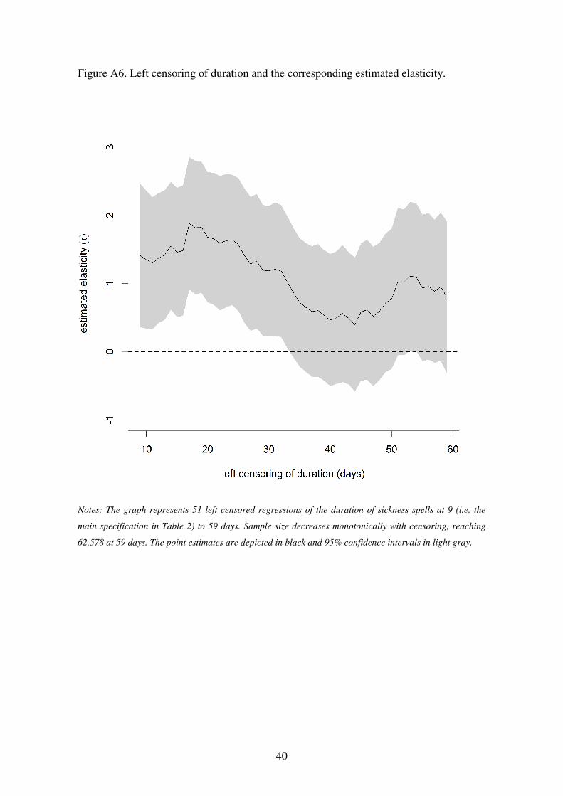
effect (see Table A3 and Figure A6). We show the results for subsamples according to

sex, left censoring of sickness spells at 20 days, and most importantly by SA criterion

and keeping only observations where the data year matches with the starting year of

sickness. When subsampled by diagnosis, sample sizes drop dramatically and all relevant

estimates are insignificant (not reported). The heterogeneity of behavior by sex or other

attributes is of no practical interest unless the policy parameters (i.e. the benefit and

contribution rules) are conditioned on these variables.

To detect whether there might be any bias induced by possible non-randomness in the

assignment, it is necessary to check for the linearity of covariates at the kink point. The

covariates are all linear, with the exception of the female indicator and the indicator for

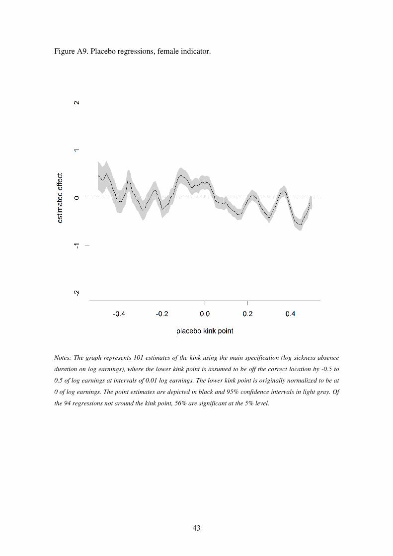
tertiary education (Table A2, Figures A7 and A8). However, we run 101 placebo

regressions, where the lower kink point is assumed to be off the correct location by -0.5

to 0.5 of log earnings at intervals of 0.01 log earnings and find nonlinearities in 56% and

49% of the specifications for the female indicator and the indicator for tertiary education,

respectively (see Figures A9 and A10). This is encouraging, since the nonlinearity of

these two variables at the lower kink point appears to be spurious, and the nonlinearities

found reflect the location of females and higher educated in the earnings distribution,

unrelated to the benefit rule.

The fact that the three most common one-letter level diagnoses are linear is particularly

important, since the diagnoses are closely linked to the duration of sickness absence. This

is evident in the R2 of the estimated regressions with and without diagnoses (Table 3).

17

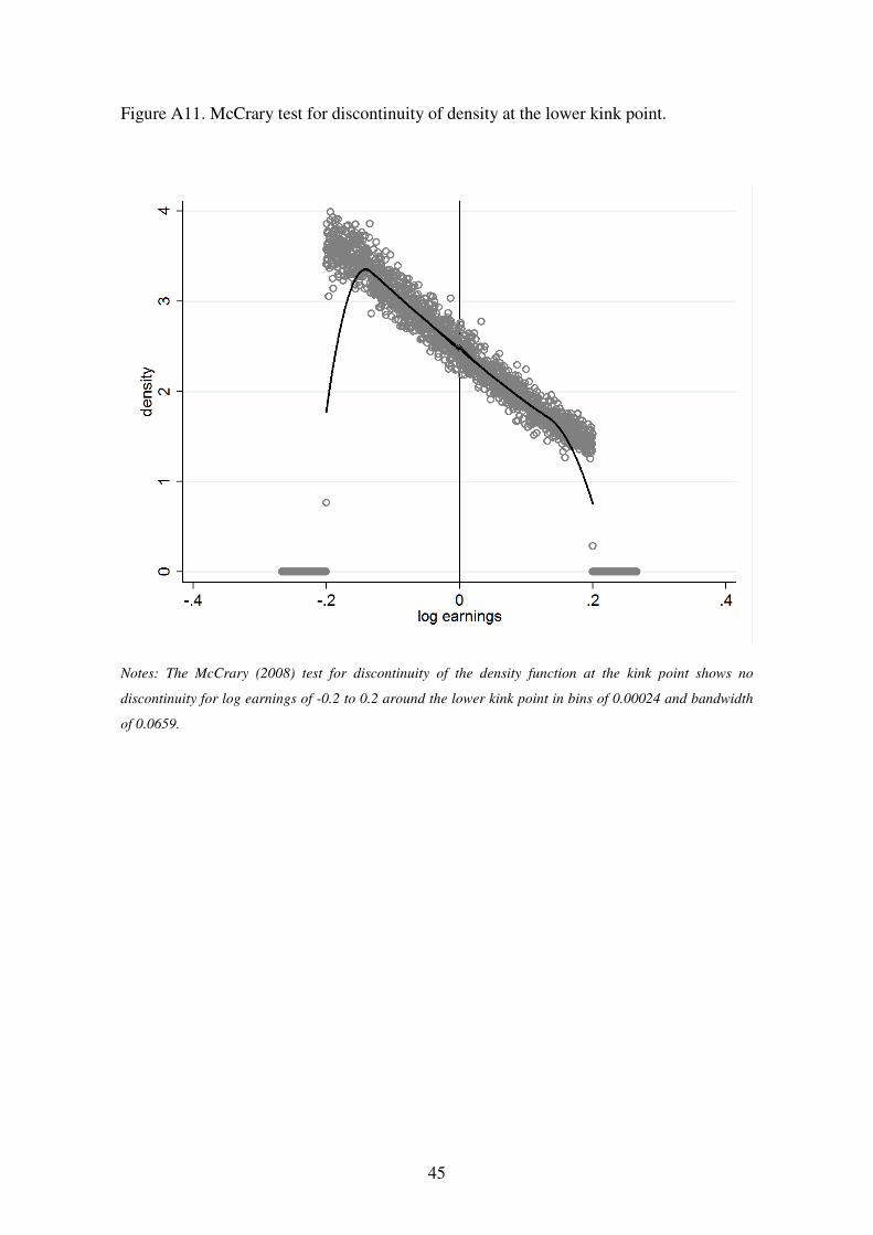
We test and find no evidence of non-smoothness in the density function of log earnings

around the lower kink point (see Figures A11 and A12).24

Neither is non-smoothness

found if the densities for males or females are considered separately (not reported).25

We

conclude that the nonlinearity of the female indicator at the kink point is of minor

concern for a causal interpretation of our response estimate.

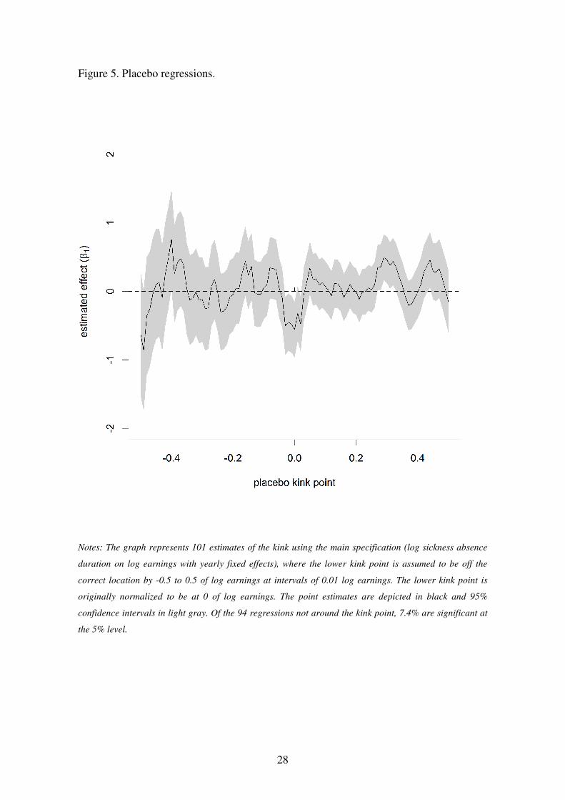
To test robustness of our main specification in Table 2, we run 101 placebo regressions

(see Figure 5).26

We use the same FG bandwidth of the true (lower) kink point for all

these regressions. Of the 94 regressions not around the true kink point, ~7 (7.4%) show a

significant estimated effect. This lends strong support to the claim that the result is not

spurious.

Figure 5 here

6.3. Economic interpretation

The response is affected in part by employer incentives (see Footnote 11 for details of the

payment structure). Using the duration of the benefit period paid out to the employer (as

opposed to the whole period, which consists periods of payments to the employer and

employee) as the response variable, the estimated response is well within the confidence

interval of our main specification. This suggests that employer incentives are aligned

with those of the employees.

As discussed in Section 2, the response parameter �� on the left-hand side of equation

(1) is the elasticity of the duration of sick leave (D) with respect to the level of sickness

benefit (B=by). In the model, the sickness benefit is financed by contributions which are

proportional to earnings, T=ty. Substituting rates for levels in the derivation of equation

(1) has no effect on the government budget constraint nor any first-order effects on the

24

We use “non-smoothness” and “bunching” interchangeably. Smoothness implies no jump in the density

or a kink in the density. 25

See Appendix 2 for a decomposition of the density function by sex. 26

Ganong and Jäger (2014) propose that researchers using RKD should present a distribution of placebo

estimates in regions without a policy kink.

18

optimal conditions and therefore the equation (1) is left unchanged (see, Chetty, 2006, p.

1884).27

In the Finnish nonlinear benefit rule, those in the higher earnings bracket receive both a

lower marginal replacement rate and a fixed benefit unrelated to earnings and created by

the nonlinear benefit rule (segment AB in Figure 6). In calculating the cost effects of

reforming the mandatory sickness insurance using our elasticity estimate we assume that

the benefit is proportionally adjusted in our policy simulation. To accomplish this we

modify all benefit rates accordingly, unchanging the locations of the kinks and therefore

proportionally adjusting also the fixed benefits (for details, see Appendix 3).

Figure 6 here

The impact of a proportional 5% increase in the benefit level for the year 2012 is a 0.06%

[0.02%, 0.11%] reduction in GDP (cf. Figure 6). For this back-of-envelope calculation,

we approximate productivity per working day by dividing annual earnings (in 2010) by

300 and adding 60% to account for indirect labor costs. The crucial (and strong)

assumption is that the estimated elasticity is constant at 1.41 [0.36, 2.46]28

throughout the

distributions of earnings, sickness benefits and sickness absence duration. We also

assume that an increase of 5% is small enough for the constancy of the elasticity.29

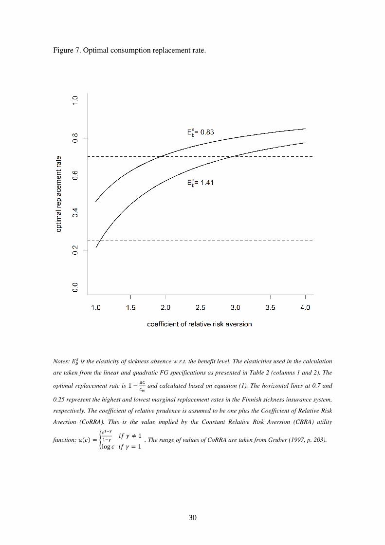
We calculate the optimal replacement rate using equation (1) and assuming a Constant

Relative Risk Aversion (CRRA) utility function (see Figure 7). Using elasticities of

absence w.r.t. the benefit level of 1.41 and 0.83, we find that the replacement rate of the

lowest bracket in the Finnish system (0.7) is optimal when the Coefficient of Relative

Risk Aversion (CoRRA) is 2.95 and 1.92, respectively, implying that the optimal

coefficient of relative prudence is 3.95 and 2.92 (see notes to Figure 7). The CoRRA may

vary with earnings level. Assuming a constant elasticity of absence throughout the

27

E.g. consider the elasticity: �� = ��U

U� = ��

�(�8)�(�8)��

�� = ��

��.

28 This estimate is based on the FG bandwidth. This is of course a local estimate for individuals at the kink

and might differ from the average response for the whole population in the presence of heterogeneity.

Specifically, our estimate corresponds to an average response weighted by the ex ante probability of being

at the kink given the distribution of unobserved heterogeneity across individuals. 29

In calculating the effects of reforming the mandatory sickness insurance by reducing the number of

benefit brackets (or extending the result to a linear benefit system with zero fixed benefit), one should in

principle take into account liquidity effects that operate through changes in non-zero fixed benefit created

by the nonlinear benefit rule (see Chetty, 2008 and Landais, 2014).

19

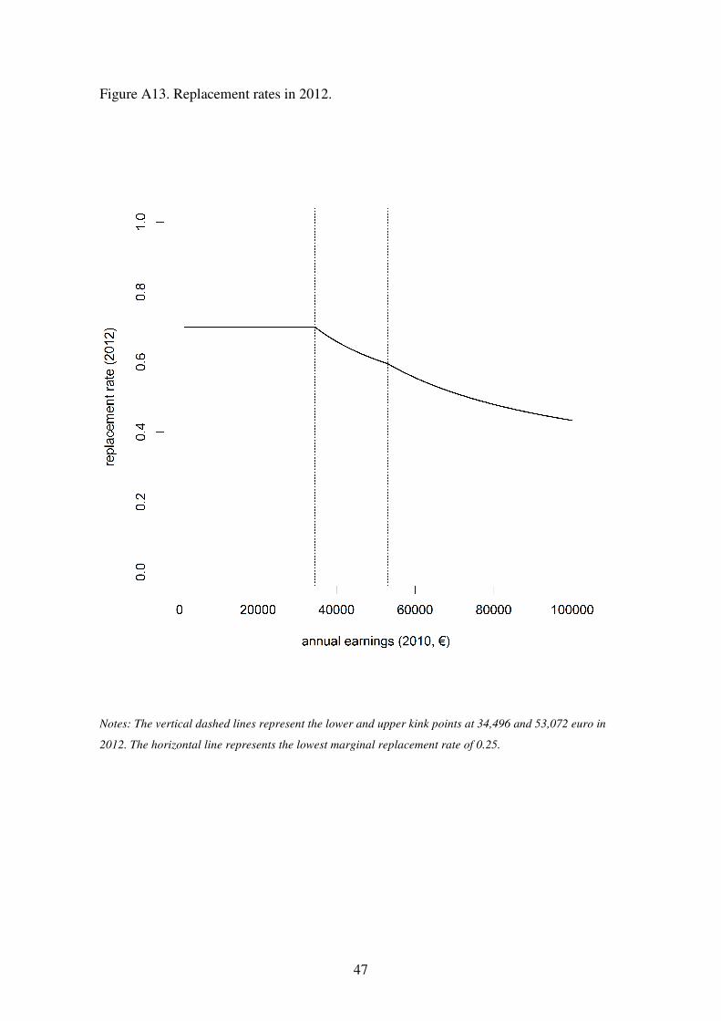
earnings distribution, the lowest replacement rates (lower bound 0.25) are optimal if

CoRRA is low at around 1 (see Figure A13 for replacement rates at different earnings

levels).

With respect to small, temporary shocks such as non-disabling illness, the CoRRA may

be much greater than w.r.t. large shocks such as disability. This difference stems from

rigidities such as consumption commitments (Chetty and Szeidl, 2006).

Figure 7 here

7. Conclusions

Using administrative data on absence spells with a large sample size, we find a

considerable incentive effect of the sickness benefit rule at the intensive margin in a

quasi-experimental research setting. The point estimate of the elasticity of the duration of

sickness absence with respect to the replacement rate is on the order of 1. Our estimate is

at the high end of those obtained in the literature using reforms (see Ziebarth and

Karlsson 2014, p. 209–210). Our research design is not subject to the same caveats as

studies exploiting reforms.

We use our elasticity estimate to characterize the optimal benefit level. In a social

insurance scheme, a decrease in the replacement rate with higher earnings can be

justified by assuming that high-income individuals have a lower risk aversion or a higher

elasticity.

Our research provides a first-rate application of the regression kink design. The research

design builds on exogenous variation that can be exploited for coherent causal inference

in a manner that the regression discontinuity design rarely offers, since the eligible

persons have significantly weaker incentives to optimize their behavior with respect to

the policy rule.

A large number of observations guarantee the robustness of our results even with

multiple controls, including sickness diagnoses. Exogeneity is ensured by the fact that the

sickness benefit is determined by earnings two years prior. An extensive battery of

20

checks was run on a number of variables which might influence our results at the kink

point. Since the estimates are obtained at the earnings level close to the median earnings

(within 1% in 2012), the response is likely to be similar for a large proportion of the

population (see Figure A2).

Previous literature on the behavioral responses to sickness benefits has analyzed reforms,

which are usually targeted at a specific subset of the population. The effect in the subset

of the population might differ from that of the total population, impairing the external

validity of these research findings.

This research delivers a compelling estimate with strong internal validity on a vital policy

parameter in a social insurance system. The result we find is crucial for policy makers

who aim to improve the mandatory sickness insurance. Future research should consider

the response at the extensive margin.

21

Figure 1. Relationship between prior annual earnings and daily sickness allowance in

euro.

Notes: The vertical dashed lines represent the discontinuity point at 1325 euro and the lower and upper

kink points at 34,496 and 53,072 euro in 2012.

22

Table 1. Descriptive statistics.

Panel A: Total sample Panel B: Sample around

the lower kink point

Mean SD Min Max Mean SD Min Max

Duration of sickness absence (days) 43.76 70.73 1 575 36.36 60.94 1 454

Duration of sickness absence (log-days) 2.76 1.47 0 6 2.62 1.42 0 6.12

Earnings 26364.68 16119.64 0 6120738 33120.44 1923.67 29095 37897

Log earnings 10.07 0.67 -3.00 15.63 10.41 0.06 10.28 10.54

Age 45.13 11.35 16 70 46.53 10.01 17 69

Female 0.59 0.49 0 1 0.48 0.5 0 1

Tertiary level education 0.14 0.34 0 1 0.16 0.36 0 1

Helsinki Metropolitan Area 0.17 0.37 0 1 0.19 0.39 0 1

Sickness allowance per day (euro) 54.3 23.19 0.01 4600.56 69.16 8.26 0.02 136.21

Panel C: Sample size by year

Year 2004 2005 2006 2007 2008 2009 2010 2011 2012 Total

Total sample 344,590 352,446 346,747 341,527 339,949 317,618 309,893 309,333 313,101 2,975,204

Sample around

the lower kink

point

39,887 41,275 41,380 40,617 40,693 38,368 37,875 37,068 37,652 354,815

Note: The sample around the lower kink point is defined within the FG bandwidth (0.0796 log euro of

annual earnings). The diagnoses M, S and F represent respectively 34, 13 and 16 percent of the whole

sample and 36, 14 and 14 percent of the sample around the lower kink point. Diagnosis M in ICD-10 refers

to diseases of the musculoskeletal system and connective tissue. Diagnosis S refers to injury, poisoning and

certain other consequences of external causes. Diagnosis F refers to mental and behavioral disorders.

23

Figure 2. Duration of sickness absence in 2012 and annual earnings.

Notes: The vertical dashed lines represent the discontinuity point at 1325 euro and the kink points at

34,496 and 53,072 euro in 2012. The dots represent the mean duration of sickness absence in bins of 800

euro. One bin between each discontinuity and the kink point has been extended such that the discontinuity

and the kink points are located at the bin cut-off points.

24

Figure 3. Duration of sickness absence (2004–2012) and annual earnings (two years

prior) around the lower kink point.

Notes: Annual earnings are deflated to 2012 prices by using the consumer price index. Earnings are in

logs and normalized to zero at the lower kink point. The dots represent the mean duration of sickness

absence in bins of 0.018 log euro. The regression fit and 95% confidence interval are shown for the FG

bandwidth (0.0796 log euro of annual earnings), which is the main specification bandwidth used in the

analysis (cf. Table 2).

25

Table 2. Regression estimates.

Panel A: Dependent variable: log duration of sickness absence (days)

Linear specification

Quadratic

specification

Linear specification,

bias-corrected (CCT)

Bandwidth FG bandwidth FG bandwidth CCT Bandwidth

Kernel Uniform Uniform Triangular

Change of slope at kink

point (?@)

-0.556***

(0.208)

-0.353***

(0.119)

..

Slope below kink point

(A@)

0.240**

(0.112)

0.162***

(0.06)

..

Yearly fixed effects Y Y N

Polynomial order 1 2 1 (bias correction: 2)

ib (Adj.) 0.0003 0.0002 ..

N 354,800 1,326,992 635,548

Panel B: Elasticity of the duration of sickness absence with respect to

replacement rate

Change in the replacement

rate ( @) -0.394***

(0.021)

-0.318***

(0.086)

-0.393***

(0.012)

Elasticity (/ ≈ [\]\) 1.411

0.830

..

Panel C: Instrumental variable estimation of the elasticity of the

duration of sickness absence with respect to replacement rate

Estimated elasticity (/) 1.411***

(0.536)

0.830***

(0.283)

1.155***

(0.359)

N 354,800 1,326,992 566,392

Notes: Heteroskedasticity-robust standard errors are reported in parentheses. Statistical significance: *

p<0.1; ** p<0.05; *** p<0.01. The main specification is marked in light grey. The estimated model is

equation (3). The FG bandwidth referring to the “rule-of-thumb” bandwidth described in Fan and Gijbels

(1996) is estimated to be 0.0796 and 0.2953 for the linear and quadratic specification, respectively. The

95% confidence interval for the IV estimated elasticity with a point estimate of 1.41 is [0.36, 2.46], using

the linear specification. CCT refers to the bandwidth (0.1416) and bias-corrected estimator proposed by

Calonico et al. (2014). The 95% confidence interval for the IV estimated elasticity with a point estimate of

1.16 is [0.45, 1.86], using the linear CCT specification. The instrument is the interaction term of past

earnings and an indicator of earnings above the lower kink point. The Angrist–Pischke first-stage F-

statistic (see Angrist and Pischke 2009, pp. 217–218) for a test of the hypothesis that the coefficient of the

instrument is zero in a regression of the received compensation on the instrument is higher (346) in the

linear FG specification than the conventional threshold of 10 for a weak instrument. Clustering standard

errors at the level of the individual increases the 95% CI only marginally (1.67%). In the main

specification, the standard error with clustering is 0.545.

26

Figure 4. Regression estimates with different bandwidths.

Notes: The graph represents 33 estimates of the elasticity (τ) using the main specification (log sickness

absence duration on log earnings with yearly fixed effects), between bandwidths of 0.0396 and 0.1996 at

intervals of 0.05 log earnings. The point estimates are depicted in black and 95% confidence intervals in

light gray. The FG bandwidth is marked by a short vertical line (cf. notes to Table 2).

27

Table 3. Regression estimates of the main specification with controls.


Change of slope at kink

point (?@)

-0.556***

(0.208)

-0.516**

(0.206)

-0.502**

(0.201)

-0.473**

(0.199)


(A@)

0.240**

(0.112)

0.055

(0.111)

0.208*

(0.108)

0.034

(0.107)

Yearly fixed effects Y Y Y Y

Individual

characteristics

Y Y

Initial diagnosis (at

one-letter level)

Y Y

Polynomial order 1 1 1 1

ib (Adj.) 0.0003 0.0134 0.0661 0.0781

N 354,800 354,800 354,800 354,800

Panel B: Instrumental variable estimation of the elasticity of the duration of sickness absence with respect to

replacement rate

Estimated elasticity (τ) 1.411***

(0.536)

1.314**

(0.533)

1.274**

(0.517)

1.206**

(0.516)

N 354,800 354,800 354,800 354,800


p<0.1; ** p<0.05; *** p<0.01. The estimated model is equation (3). Individual characteristics are age,

sex, the Helsinki Metropolitan Area indicator and tertiary education indicator. Initial diagnosis is denoted

at the one-letter level, following the International Statistical Classification of Diseases and Related Health

Problems 10th Revision (ICD-10). The data have 21 different values for this variable. The FG bandwidth

referring to the “rule-of-thumb” bandwidth described in Fan and Gijbels (1996) is estimated to be 0.0796.

The instrument is the interaction term of past earnings and an indicator of earnings above the lower kink

point. The lowest Angrist–Pischke first-stage F-statistic for a test of the hypothesis that the coefficient of

the instrument is zero in a regression of the received compensation on the instrument is 344 in the second

column regression with individual characteristics as the control variables (cf. notes in Table 2).

28

Figure 5. Placebo regressions.

Notes: The graph represents 101 estimates of the kink using the main specification (log sickness absence

duration on log earnings with yearly fixed effects), where the lower kink point is assumed to be off the

correct location by -0.5 to 0.5 of log earnings at intervals of 0.01 log earnings. The lower kink point is

originally normalized to be at 0 of log earnings. The point estimates are depicted in black and 95%

confidence intervals in light gray. Of the 94 regressions not around the kink point, 7.4% are significant at

the 5% level.

29

Figure 6. A policy reform.

Notes: #(%) is the benefit rule. j = 1.05.

30

Figure 7. Optimal consumption replacement rate.

Notes: �� is the elasticity of sickness absence w.r.t. the benefit level. The elasticities used in the calculation

are taken from the linear and quadratic FG specifications as presented in Table 2 (columns 1 and 2). The

optimal replacement rate is 1 − ∆�� and calculated based on equation (1). The horizontal lines at 0.7 and

0.25 represent the highest and lowest marginal replacement rates in the Finnish sickness insurance system,

respectively. The coefficient of relative prudence is assumed to be one plus the Coefficient of Relative Risk

Aversion (CoRRA). This is the value implied by the Constant Relative Risk Aversion (CRRA) utility

function: m(n) = op\qr@3] HI ≠ 1log n HI = 1. The range of values of CoRRA are taken from Gruber (1997, p. 203).

31

Appendix 1: Additional figures and tables.

Figure A1. Annual earnings and compensation level around the lower kink point in 2012.

Notes: Earnings are in logs and normalized to zero at the lower kink point. The large dots represent the

mean log compensation level in bins of 0.006 log euro. Each small dot represents one observation. The

vertical axis has been cut at 4.5 for clarity. The regression fit and 95% confidence interval are shown for

the FG bandwidth (0.0796 log euro of annual earnings), which is the main specification bandwidth used in

the analysis. The double line that starts right below the lower kink point stems from the fact that some of

the benefits in 2012 data follow 2011 replacement rates. This is a source of fuzziness in the data.

32

Figure A2. Kernel density estimates of the earnings distributions.

Notes: The vertical dashed lines represent the discontinuity points at 1,211 and 1,325 euro and the kink

points at 31,506 and 48,473 euro in dark gray (2002) and 34,496 and 53,072 euro in black (2010). The

kernel is Gaussian and the bandwidth is set at 675 and 769 euro, respectively.

33

Figure A3. Duration of sickness absence (2004–2012) and annual earnings (two years

prior) around the lower kink point, with the dot size representing sample size within the

bin.



absence in bins of 0.018 log euro. The dot size represents sample size within the bin, from the highest

(57,341) to the lowest (25,194).

34

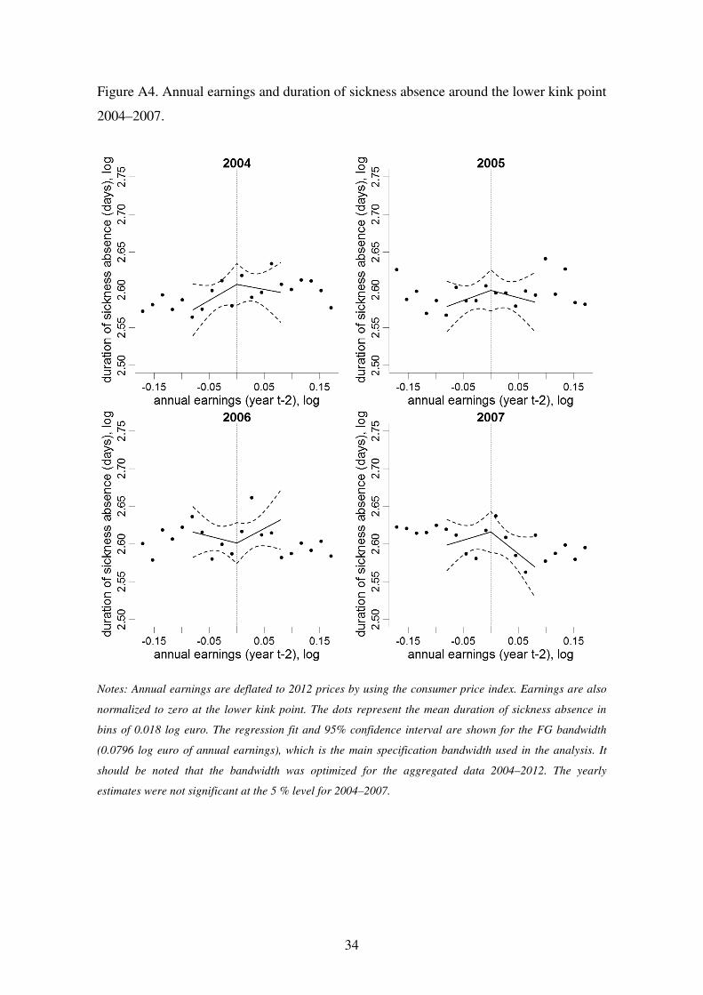
Figure A4. Annual earnings and duration of sickness absence around the lower kink point

2004–2007.

Notes: Annual earnings are deflated to 2012 prices by using the consumer price index. Earnings are also

normalized to zero at the lower kink point. The dots represent the mean duration of sickness absence in

bins of 0.018 log euro. The regression fit and 95% confidence interval are shown for the FG bandwidth

(0.0796 log euro of annual earnings), which is the main specification bandwidth used in the analysis. It

should be noted that the bandwidth was optimized for the aggregated data 2004–2012. The yearly

estimates were not significant at the 5 % level for 2004–2007.

35

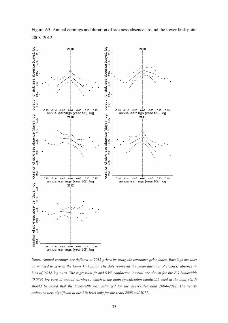
Figure A5. Annual earnings and duration of sickness absence around the lower kink point

2008–2012.

Notes: Annual earnings are deflated to 2012 prices by using the consumer price index. Earnings are also

normalized to zero at the lower kink point. The dots represent the mean duration of sickness absence in

bins of 0.018 log euro. The regression fit and 95% confidence interval are shown for the FG bandwidth

(0.0796 log euro of annual earnings), which is the main specification bandwidth used in the analysis. It

should be noted that the bandwidth was optimized for the aggregated data 2004–2012. The yearly

estimates were significant at the 5 % level only for the years 2008 and 2011.

36

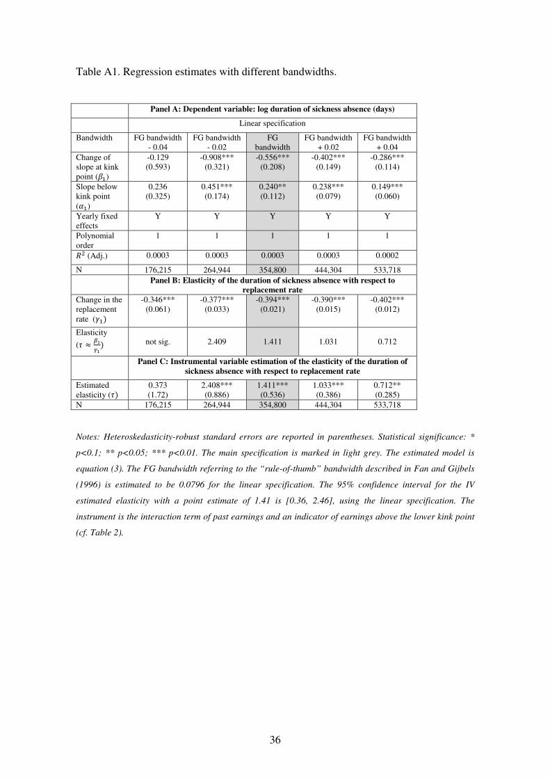
Table A1. Regression estimates with different bandwidths.


Linear specification

Bandwidth FG bandwidth

- 0.04

FG bandwidth

- 0.02

FG

bandwidth

FG bandwidth

+ 0.02

FG bandwidth

+ 0.04

Change of

slope at kink

point (?@)

-0.129

(0.593)

-0.908***

(0.321)

-0.556***

(0.208)

-0.402***

(0.149)

-0.286***

(0.114)

Slope below

kink point

(A@)

0.236

(0.325)

0.451***

(0.174)

0.240**

(0.112)

0.238***

(0.079)

0.149***

(0.060)

Yearly fixed

effects

Y Y Y Y Y

Polynomial

order

1 1 1 1 1

ib (Adj.) 0.0003 0.0003 0.0003 0.0003 0.0002

N 176,215 264,944 354,800 444,304 533,718

Panel B: Elasticity of the duration of sickness absence with respect to

replacement rate

Change in the

replacement

rate ( @) -0.346***

(0.061)

-0.377***

(0.033)

-0.394***

(0.021)

-0.390***

(0.015)

-0.402***

(0.012)

Elasticity

(/ ≈ [\]\) not sig.

2.409

1.411

1.031

0.712

Panel C: Instrumental variable estimation of the elasticity of the duration of

sickness absence with respect to replacement rate

Estimated

elasticity (/) 0.373

(1.72)

2.408***

(0.886)

1.411***

(0.536)

1.033***

(0.386)

0.712**

(0.285)

N 176,215 264,944 354,800 444,304 533,718


p<0.1; ** p<0.05; *** p<0.01. The main specification is marked in light grey. The estimated model is

equation (3). The FG bandwidth referring to the “rule-of-thumb” bandwidth described in Fan and Gijbels

(1996) is estimated to be 0.0796 for the linear specification. The 95% confidence interval for the IV

estimated elasticity with a point estimate of 1.41 is [0.36, 2.46], using the linear specification. The

instrument is the interaction term of past earnings and an indicator of earnings above the lower kink point

(cf. Table 2).

37

Table A2. Regression estimates from the main local linear specification, covariates.

Bandwidth FG bandwidth

- 0.04

FG bandwidth

- 0.02

FG bandwidth FG bandwidth

+ 0.02

FG bandwidth

+ 0.04

Diagnose M

Change of

slope at kink

point (?@)

0.007

(0.2)

-0.127

(0.108)

0.006

(0.07)

-0.021

(0.05)

-0.040

(0.038)

ib (Adj.) 0.0002 0.0003 0.0004 0.0004 0.0005

N 176,215 264,944 354,800 444,304 533,718

Diagnose S

Change of

slope at kink

point (?@)

-0.023

(0.145)

0.051

(0.079)

0.004

(0.051)

0.033

(0.037)

-0.018

(0.028)

ib (Adj.) 0.0002 0.0002 0.0002 0.0003 0.0004

N 176,215 264,944 354,800 444,304 533,718

Diagnose F

Change of

slope at kink

point (?@)

-0.050

(0.145)

-0.008

(0.079)

0.045

(0.051)

0.009

(0.036)

0.001

(0.028)

ib (Adj.) 0.0004 0.0003 0.0002 0.0002 0.0002

N 176,215 264,944 354,800 444,304 533,718

Diagnose M, S or F

Change of

slope at kink

point (?@)

-0.065

(0.2)

-0.085

(0.109)

0.055

(0.07)

0.021

(0.05)

-0.057

(0.039)

ib (Adj.) 0.0005 0.0005 0.0006 0.0005 0.0005

N 176,215 264,944 354,800 444,304 533,718

Age

Change of

slope at kink

point (?@)

3.403

(4.144)

-2.517

(2.262)

0.568

(1.464)

2.117**

(1.046)

2.667***

(0.798)

ib (Adj.) 0.0008 0.0009 0.0009 0.0011 0.0012

N 176,215 264,944 354,800 444,304 533,718

Female

Change of

slope at kink

point (?@)

0.437**

(0.208)

0.494***

(0.113)

0.312***

(0.073)

0.318***

(0.052)

0.353***

(0.04)

ib (Adj.) 0.0037 0.0057 0.0085 0.0118 0.0152

N 176,215 264,944 354,800 444,304 533,718

Female (quadratic specification)

Change of

slope at kink

point (?@)

-0.002

(0.829)

0.180

(0.450)

0.638**

(0.291)

0.450**

(0.207)

0.316**

(0.157)

ib (Adj.) 0.0037 0.0057 0.0085 0.0118 0.0152

N 176,215 264,944 354,800 444,304 533,718

Highest Degree Tertiary Education

Change of

slope at kink

point (?@)

0.003

(0.151)

0.210**

(0.083)

0.134**

(0.054)

0.131***

(0.038)

0.152***

(0.029)

38

ib (Adj.) 0.0068 0.0076 0.0080 0.0087 0.0101

N 176,215 264,944 354,800 444,304 533,718

Highest Degree Tertiary Education (quadratic specification)

Change of

slope at kink

point (?@)

-0.156

(0.605)

-0.404

(0.329)

0.062

(0.212)

0.135

(0.151)

0.104

(0.115)

ib (Adj.) 0.0068 0.0076 0.0080 0.0087 0.0101

N 176,215 264,944 354,800 444,304 533,718

Lives in Helsinki Metropolitan Area

Change of

slope at kink

point (?@)

-0.083

(0.164)

0.0270

(0.089)

-0.051

(0.058)

0.001

(0.041)

0.031

(0.032)

ib (Adj.) 0.0001 0.0004 0.0005 0.0007 0.0010

N 176,215 264,944 354,800 444,304 533,718


p<0.1; ** p<0.05; *** p<0.01. The estimated model is equation (3). Diagnosis M in ICD-10 refers to

diseases of the musculoskeletal system and connective tissue. Diagnosis S refers to injury, poisoning and

certain other consequences of external causes. Diagnosis F refers to mental and behavioral disorders. The

FG bandwidth referring to the “rule-of-thumb” bandwidth described in Fan and Gijbels (1996) is

estimated to be 0.0796.

39

Table A3. Regression estimates for different subsamples.


Subsample Females Males Left censoring

at 20 days

SA criterion:

annual

earnings year

t-2

Observations

where the data

year matches

with the starting

year of sickness

Change of slope at

kink point (?@)

-0.110

(0.293)

-0.779***

(0.294)

-0.705***

(0.177)

-0.488**

(0.223)

-0.501**

(0.227)


(A@)

0.077

(0.153)

0.059

(0.162)

0.350***

(0.095)

0.205*

(0.120)

0.221*

(0.122)

Yearly fixed effects Y Y Y Y Y

Polynomial order 1 1 1 1 1

ib (Adj.) 0.0001 0.0011 0.0003 0.0003 0.0004

N 170,869 183,931 204,208 306,463 296,907

Panel B: Elasticity of the duration of sickness absence with respect to replacement rate

Change in the

replacement rate ( @) -0.406***

(0.030)

-0.384***

(0.030)

-0.386***

(0.032)

-0.380***

(0.022)

-0.415**

(0.012)

Elasticity (/ ≈ [\]\) 0.271

2.029

1.826

1.284

1.207

Panel C: Instrumental variable estimation of the elasticity of the duration of sickness

absence with respect to replacement rate

Estimated elasticity (/) 0.271

(0.724)

2.032***

(0.790)

1.823***

(0.491)

1.286**

(0.595)

1.206**

(0.553)

N 170,869 183,931 204,208 306,463 296,907


p<0.1; ** p<0.05; *** p<0.01. The bandwidth is the FG bandwidth of the main specification (see Table 2

for more details).

40

Figure A6. Left censoring of duration and the corresponding estimated elasticity.

Notes: The graph represents 51 left censored regressions of the duration of sickness spells at 9 (i.e. the

main specification in Table 2) to 59 days. Sample size decreases monotonically with censoring, reaching

62,578 at 59 days. The point estimates are depicted in black and 95% confidence intervals in light gray.

41

Figure A7. Linearity of covariates: initial diagnoses.





analysis. Diagnosis M in ICD-10 refers to diseases of the musculoskeletal system and connective tissue.

Diagnosis S refers to injury, poisoning and certain other consequences of external causes. Diagnosis F

refers to mental and behavioral disorders.

42

Figure A8. Linearity of covariates: age, sex (female indicator), having tertiary education

and living in the Helsinki Metropolitan Area.





analysis.

43

Figure A9. Placebo regressions, female indicator.


duration on log earnings), where the lower kink point is assumed to be off the correct location by -0.5 to

0.5 of log earnings at intervals of 0.01 log earnings. The lower kink point is originally normalized to be at

0 of log earnings. The point estimates are depicted in black and 95% confidence intervals in light gray. Of

the 94 regressions not around the kink point, 56% are significant at the 5% level.

44

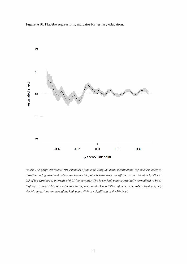
Figure A10. Placebo regressions, indicator for tertiary education.


duration on log earnings), where the lower kink point is assumed to be off the correct location by -0.5 to

0.5 of log earnings at intervals of 0.01 log earnings. The lower kink point is originally normalized to be at

0 of log earnings. The point estimates are depicted in black and 95% confidence intervals in light gray. Of

the 94 regressions not around the kink point, 49% are significant at the 5% level.

45

Figure A11. McCrary test for discontinuity of density at the lower kink point.

Notes: The McCrary (2008) test for discontinuity of the density function at the kink point shows no

discontinuity for log earnings of -0.2 to 0.2 around the lower kink point in bins of 0.00024 and bandwidth

of 0.0659.

46

Figure A12. An adapted McCrary test for discontinuity of the slope of the density at the

lower kink point.

Notes: A test for a kink (i.e. a discontinuity in the slope) of the density function at the kink point shows no

discontinuity in the slope, adapting the McCrary test for slopes using bins of 0.00024 and bandwidth of

0.0659.

47

Figure A13. Replacement rates in 2012.

Notes: The vertical dashed lines represent the lower and upper kink points at 34,496 and 53,072 euro in

2012. The horizontal line represents the lowest marginal replacement rate of 0.25.

48

Appendix 2: The density function by sex.

Consider a mixed density by sex ( ) ( ) (1 ) ( )m m m f

f y p f y p f y= + − , and probability

( )( ) ( | ) ( ) ( ) (1 ) ( )m m m m m m fP y P sex m y p f y p f y p f y= = = + − , then

( ) ( ) ( )m m mp f y P y f y= .

By differentiation, ( )( ) ( ) ( )( ) ( ) ( ) ( ) ( ), { , }j m m j m m jD p f y D P y f y P y D f y j= + ∈ + − . If

( ) ( )( ) ( )k ky yD f y D f y

+ −= and lim ( ) lim ( )

k ky y y yf y f y

− +→ →

= ( )0mp > , then

0 0 0 0( ) ( ) ( ) ( )( ) ( ) ( ) ( )m y m y m y m yD f y D f y D P y D P y+ − + −

= ⇔ = .

Appendix 3: A policy simulation.

In a nonlinear benefit rule those in the higher earnings bracket receive both a lower

marginal replacement rate and the fixed benefit created by the nonlinear benefit rule

(segment AB in Figure 6). However, this does not correspond to a lump-sum benefit

since total benefit depends on the duration of sick leave. In calculating the cost effects of

reforming the mandatory sickness insurance by changing the number or locations of the

benefit brackets, one should take into account the effect that operates through changes in

non-zero fixed benefit created by the nonlinear benefit rule.

! = (#b(u − u@)+#@u@)1(u − u@) + #@u@1(u@ − u)

On the upper segment, u > u@, agent receives benefit !b1,!b = #b(u − u@) + #@u@ =#bu + (#@ − #b)u@with fixed rate benefit !B = (#@ − #b)u@. The consumption while on

sick leave, �� = v + !1 + u(1 − 1), and v is the prior level of assets which affects the

liquidity constraint. Similarly, the agent pays tax to finance benefits according to a linear

schedule w = xu, while working. The consumption while working, �� = v + u − w.

The above formulae hold in the lower segment, u ≤ u@ with #b = #@.

49

A proportional increase in all marginal replacement rates in the benefit system gives

j! = (j#b(u − u@)+j#@u@)1(u − u@) + j#@u@1(u@ −u), resulting in a proportional

increase in the fixed rate benefit on the upper segment (segment AC in Figure 6):

j!b = (j#bu + j(#@ − #b)u@)1(u − u@), and j!@ = j#@u1(u@ − u).

References

Aittomäki, A., Martikainen, P., Rahkonena, O. and Lahelma, E. (2014). Household

income and health problems during a period of labour-market change and widening

income inequalities – a study among the Finnish population between 1987 and 2007.

Social Science and Medicine, 100, 84–92.

Angrist, J.D. and Pischke, J.S. (2009). Mostly Harmless Econometrics: An Empiricist’s

Companion. Princeton University Press, Princeton.

Baily, M.L. (1978). Some aspects of optimal unemployment insurance. Journal of Public

Economics, 10, 379–402.

Besley, T. and Case, A. (2000). Unnatural experiments? Estimating the incidence of

endogenous policies. Economic Journal, 110, F672–F694.

Calonico, S., Cattaneo, M.D. and Titiunik, R. (2014). Robust nonparametric confidence

intervals for regression-discontinuity designs. Econometrica, 82, 2295–2326.

Card, D., Lee, D., Pei, Z. and Weber, A. (2012). Nonlinear policy rules and the

identification and estimation of causal effects in a generalized regression kink design.

NBER Working Paper No. 18564.

Chetty, R. (2006). A general formula for the optimal level of social insurance. Journal of

Public Economics, 90, 1879–1901.

Chetty, R. (2008). Moral hazard versus liquidity and optimal unemployment insurance.

Journal of Political Economy, 116, 173–234.

50

Chetty, R. and Saez, E. (2010). Optimal taxation and social insurance with endogenous

private insurance. American Economic Journal: Economic Policy, 2, 85–114.

Chetty, R. and Szeidl, A. (2007). Consumption commitments and risk preferences.

Quarterly Journal of Economics, 122, 831–877.

De Paola, M., Scoppa, V. and Pupo, V. (2014). Absenteeism in the Italian public

sector: The effects of changes in sick leave policy. Journal of Labor Economics, 32, 337–

360.

DICE Database (2012). Lost working time due to sickness, 2000-2009. Ifo Institute,

Munich, online available at http://www.cesifo-group.de/DICE/fb/3Sb8mxDdU

Eurostat (2011). The European System of integrated Social Protection Statistics

(ESSPROS). Methodologies and Working papers.

Fan, J. and Gijbels, I. (1996). Local Polynomial Modelling and Its Applications.

Chapman and Hall, London.

Fevang, E., Markussen S. and Røed, K. (2014). The sick pay trap. Journal of Labor

Economics, 32, 305–366.

Frick, B. and Malo, M.A. (2008). Labor market institutions and individual absenteeism in

the European Union: The relative importance of sickness benefit systems and

employment protection legislation. Industrial Relations, 47, 505–529.

Ganong, P. and Jäger, S. (2014). A permutation test and estimation alternatives for the

regression kink design. IZA Discussion Paper No. 8282.

Gelman, A. and Imbens, G. (2014). Why high-order polynomials should not be used in

regression discontinuity designs. NBER Working Paper No. 20405.

51

Gimeno, D., Benavides, F.G., Benach, J. and Amick, III B.C. (2004). Distribution of

sickness absence in the European Union countries. Occupational and Environmental

Medicine, 61, 867–869.

Gruber, J. (1997). The consumption smoothing benefits of unemployment insurance. The

American Economic Review, 87, 192–205.

Gruber, J. (2000). Disability insurance benefits and labor supply. Journal of Political

Economy, 108, 1162–1183.

Henrekson, M. and Persson, M. (2004). The effects on sick leave of changes in the

sickness insurance system. Journal of Labor Economics, 22, 87–113.

Imbens, G. W. and Lemieux, T. (2008). Regression discontinuity designs: A guide to

practice. Journal of Econometrics, 142, 615–635.

Johansson, P. and Palme, M. (2005). Moral hazard and sickness insurance. Journal of

Public Economics, 89, 1879–1890.

Kangas, O., Niemelä, M. and Varjonen, S. (2013). Politics in the making of sickness

insurance in Finland. In Haggrén, H., Rainio-Niemi, J. and Vauhkonen, J. (Eds.): Multi-

layered Historicity of the Present: Approaches to Social Science History. University of

Helsinki, Helsinki, pp. 271–296.

Kivimäki, M., Forma, P., Wikström, J., Halmeenmäki, T., Pentti, J., Elovainio, M., and

Vahtera, J. (2004). Sickness absence as a risk marker of future disability pension: the 10-

town study. Journal of Epidemiology and Community Health, 58, 710–711.

Landais, C. (2014). Assessing the welfare effects of unemployment benefits using the

regression kink design. American Economic Journal: Economic Policy, Forthcoming.

Lee, D.S., and Lemieux, T. (2010). Regression discontinuity designs in economics.

Journal of Economic Literature, 48, 281–355.

52

Lehto, A-M and Sutela, H. (2009). Three Decades of Working Conditions. Findings of

Finnish Quality of Work Life Surveys 1977–2008. Statistics Finland, Helsinki.

MaCurdy, T.E. (1981). The empirical model of labor supply in a life-cycle model.

Journal of Political Economy, 89, 1059–1085.

McCrary, J. (2008). Manipulation of the running variable in the regression discontinuity

design: A density test. Journal of Econometrics, 142, 698–714.

Nielsen, H. S., Sørensen, T. and Taber, C. (2010). Estimating the effect of student aid on

college enrollment: Evidence from a government grant policy reform. American

Economic Journal: Economic Policy, 2, 185–215.

Pettersson-Lidbom, P. and Skogman Thoursie, P. (2013). Temporary disability insurance

and labor supply: Evidence from a natural experiment. Scandinavian Journal of

Economics, 115, 485–507.

Puhani, P.A. and Sonderhof, K. (2010). The effects of a sick pay reform on absence and

on health-related outcomes. Journal of Health Economics, 29, 285–302.

Treble, J. and Barmby, T. (2011). Worker Absenteeism and Sick Pay. Cambridge

University Press, Cambridge.

Sturges, H. (1926). The choice of a class-interval. Journal of the American Statistical

Association, 21, 65–66.

Toivonen, L. (2012). Statutory and occupational sickness benefits in Finland in 2011.

Kela Online Working Paper No. 34/2012.

Ziebarth, N.R. and Karlsson, M. (2014). The effects of expanding the generosity of the

statutory sickness insurance system. Journal of Applied Econometrics, 29, 208–230.

a kink that makes you sick: the effect of sick pay on absence in a social insurance system

Government & Nonprofit

labour institute

research purposes

finland telephone

government institute

administrative register

helsinki puh

replication purposes

incentive effect of