A Library

L E D A

of Efficient Data Types and Algorithms

Kurt Mehlhorn and Stefan N£her

Fachbereich Informatik, Universit£t des $aarlandes D-6600 Saarbrfcken, Federal Republic of Germany

A b s t r a c t

LEDA is a library of efficient data types and algorithms. At present, its strength is graph algorithms and the data structures related to them. The computational geometry part is evolving. The main features of the library are 1) a clear separation of specification and implementation 2) parameterized data types 3) a comfortable data type graph, and 4) its ease of use.

I. Introduct ion

There is no standard library of the data structures and algorithms of combinatorial computing. This is in sharp contrast to many other areas of computing. There are e.g. packages in statistics (SPSS), numerical analysis (LINPACK, EISPACK), symbolic computation (MACSYMA, SAC-2) and linear programming (MPSX).

In fact the situation is worse, since even within small groups, say the algorithms group at our home institution, software is frequently not shared. Rather, each researcher starts from scratch and e.g. develops his own version of a balanced tree. Of course, this continuous "reimplementation of the wheel" slows down progress, within research and even more so outside. This is due to the fact that outside research the investment for implementing an efficient solution is frequently not made, because it is doubtful whether the implementation can be reused, and therefore methods which are known to be less efficient are used instead. Thus the scientific discoveries migrate only slowly into practice.

One of the major differences between combinatorial computing and other areas of com- puting such as statistics, numerical analysis and linear programming is the usage of complex data types. Whilst the built-in types, such as integers, reals, vectors, matrices

89

and functions, usually suffice in the other areas, combinatorial computing heavily relies on types like stacks, queues, dictionaries, sequences, sorted sequences, priority queues, graphs, points, planes, . . . .

One year ago, we started a project (called LEDA for Library of Efficient Data types and Algorithms) to build a small, but growing library of data types and algorithms in a form which allows them to be used by non-experts. We hope that the system will narrow the gap between algorithms research, teaching, and implementation. In this paper we report on our difficulties and achievements. The main features of the library are:

1) A clear separation between (abstract) data types and the data structures used to implement them, cf. section IL This distinction is frequently not made in the combinatorial algorithms literature, but it is crucial for a library. Note that we stated above that each researcher implemented its own version of a balanced tree, i.e. a data structure, and not its own version of a dictionary, i.e. a data type. The data types currently available are stack, queue, list, set, dictionary, ordered sequence, priority queue, directed graph and undirected graph. The most difffcult decision, which we faced, was the treatment of positions and pointers. For the efficiency of many data structures it is crucial that some operations on the data structure take positions in (= pointers into) the data structure as arguments. We have chosen an item concept to cast the notion of position into an abstract form, cf. section II.

2) Type parameters, cf. section II. Most of our data types have type parameters. For example, a dictionary has a key type K and an information type I and a specific dictionary type is obtained by setting, say, K to int and I to real.

3) A comfortable data type graph. It offers the standard iterations such as "for all nodes v of a graph G do" (written foraU_nodes(v, G)) or "for all neighbors w of v do" (written forall_adj_nodes(w, v)), it allows to add and delete vertices and edges and it offers arrays and matrices indexed by nodes and edges,..., cf. section III for details. The data type graph permits to write programs for graph problems in a form close to the way the algorithms are usually presented in text books. Section VII contains a list of the algorithms which are currently in LEDA.

4) Ease of use: LEDA is written in C + + (cfront version 1.2.1). All data types and algorithms are precompiled modules which can be linked with application programs. All examples given in this paper show executable code.

This paper is organized as follows. In section II we discuss data types and data struc- tures, in section III the data type graph and in section IV we discuss the interaction of graphs and data types. In section V we briefly discuss the internal structure of LEDA and in section VI we report about our experiences with designing, implementing and using LEDA.

The design of LEDA is joint work by the two authors, the implementation was mostly done by the second author. LEDA is available from the authors for a handling charge of DM 100.

90

II. Data types

One of the major differences between combinatorial computing and other areas of com- puting such as statistics, numerical analysis and linear programming is the usage of complex data types. Whilst the built-in types, such as integers, reals, vectors, matrices and functions, usually suffice in the other areas, combinatorial computing heavily relies on types like stacks, queues, dictionaries, sequences, sorted sequences, priority queues, graphs, points, planes, . . . . Even modern programming languages do not provide these types and hence they have to be defined and implemented by the individual user. A sig- nificant improvement would result, if these data types were made available as "packages" by some users and could then be reused by others. Of course, this requires to specify the properties of the data type independently of the implementation. We next discuss the LEDA specification of the data types dictionary, priority queue and partition.

E x a m p l e 1, D ic t iona ry : A dictionary is a partial function with finite domain from some universe K of keys into some set I of informations associated with the keys. An access operation looks up the function value at an argument, an insert extends the domain of definition, ... . Thus a clean definition of the data type dictionary is avail- able and hence a dictionary module should cause no principal difficulties. In fact, the programming language Comskee [BKMRS84] includes the dictionary among its built- in data types. A (minor) problem ties in the fact that most programming languages force the user to edit source text when he wants to change the key or information type. This problem is resolved in languages such as Clu or C++. Program 1 shows a small illustration of LEDA's dictionary modul.

(1) C2) (3) (4) (5) (6) (7) (s) (9) (10) (11) (12)

# include <LEDA/dictionary.h>

declare2(dictionary, int,int); main() { dictionary(int,int) D;

int k; whi le (cin > > k) ( if (D.defined(k))

I / K = x =int

D.change_inf( k,D.lookup ( k ) + l ) ; else D.insert(k,1);

} forall_keys(k,D) cout < < k < < ~'" < < D.lookup(k) < < "\ n ' ;

} P r o g r a m 1: Counting the number of occurences of each element of a sequence of

integers

P r o g r a m l

The program reads a sequence of integers and counts the number of occurences of each integer in the sequence. The number of occurences is then listed for each integer in the sequence. The details are as follows. Line (1) includes LEDA's dictionary modul.

9]

In line (2) the dictionary type dictionary(int,int) is defined. Note that the dictionary module provides dictionaries from K to I where K and I are type variables. A specific dictionary type is introduced as shown in line (2). Line (4) introduces D as the name of an object of type dictionary(int,int); D is initialized with the empty function. Line (6) to (10) step through the input sequence. In line (7) we test whether k belongs to the domain of D and then either increase the value at argument k by one or insert the pair (k,1) into the dictionary. Finally, line (11) steps through all keys k in the domain of D and prints k and the value of D at k.

LEDA is written in C + ÷ which is an extension of the C programming language. In addition to the facilities of C, C + + provides data abstraction, data hiding, object based programming, operator overloading and many other features suitable for implementing abstract data types. For details of the C + + language see "The C + + Programming Language" [St86]. Every data type in LEDA is implemented as a C + + class which is a user defined type similar to a record type in PASCAL or a struct type in C. The members of a class in C + + are not only data fields (as in C or PASCAL) they can also be functions. We use these member functions to realize the operations on the corresponding data type. Member functions are invoked using the known syntax for record field or structure member access: Let D be an object (variable) of a class with a member functions f() then D.f() calls f for D.

E x a m p l e 2~ P r io r i t y Queues: Priority queues are frequently used in network al- gorithms; cfi section III for an example. It is tempting to define a priority queue as a dictionary with the additional operations findmin and deerease_inf (We require a linear order on I). The operation PQ.findmin 0 returns the element v in the domain of PQ with minimal function value and PQ.decrease_inf(v, i) decreases the function value at argument v to i. The operation raises an error if i is larger than the old value at argument v. It is clear that a decreaseinf operation involves a lookup and hence must be at least as costly as a lookup operation in a dictionary. However, several recent papers, e.g. [FT84] and [AMOT88] show that the decrease_inf operation can be realized in time O(1) if its argument is the position of the pair (v, PQ(v)) in the data structure realizing the priority queue PQ. This led to improvements in several network algorithms.

We conclude that the argument of a decreaseAnf operation cannot be the key v. But what should it be? It cannot be the position in a data structure since we want to clearly separate data type and data structure and therefore cannot use a notion of the particular implementation in the definition of the data type. What we need is an abstraction of position.

In LEDA, we call an abstract position an i~em. For most data types XYZ there is also a type XYZ_item. This type represents the set of positions in objects of data type XYZ. So, together with the data type priority_queue there is also a type priority_queue_item or briefly pq_itern. Each pq_itcrn contains or has associated with it a pair (v, i) with v E K and i E I. We use < v, i > to denote the item which contains the pair (v, i). A priority queue PQ over K and I is then nothing but a collection of pq_iterns where each item contains a pair (v, i).

R e m a r k 1: In mathematical terms a priority queue in LEDA is simply a partial func- tion from the set of pqAtems to the cartesian product K × I. In computer science

92

terminology, we may view a pq_item as the name (&-- address) of a container holding an argument-value pair (v, i).

R e m a r k 2: Access by position can now be achieved as follows. When we insert a pair (v,i) into a priority queue PQ, the operation PQ.insert(v, i) returns an item, say it, i.e. the name of a container which holds the pair (v, i). The user of the priority queue remembers this name and can now access the pair (v, i) in two different ways. He can either access it through the item it which was returned by the insert (this is access by position) or through the key v (this is access by key). There is a crucial difference between the two modes of access. In the latter case, the key v identifying the pair (v,i) was provided by the user and hence access involves a dictionary look-up, in the former case, the name it identifying the pair (v, i) was produced by the machine and therefore can give direct access. The decreaseinf operation uses access by position, i.e. whenever the user wants to decrease the value asociated with v, he calls PQ.decrease_inf and gives it the name of the container as an argument. In this way, the item concept captures the notion of access by position but is nevertheless independent of implementation.

The complete LEDA specification of the data type priority queue follows.

A p r io r i ty queue Q is collection of items (predefined type "pq_item'). Every item contains a key from a type K and an information from a type I. K is called the key type of Q and I is called the information type of Q. The number of items in Q is called the size of Q. If Q has size zero it is called the empty priority queue. We use < k, i > to denote the pq_item with key k and information i. There must exist a total ordering "<" on I.

1. Dec l a r a t i on of a p r io r i ty queue t y p e

declare2 (priority _queue,K,I)

introduces a new data type with name "priority_queue(K,I)" consisting of all priority queues with key type K and information type I.

2. Dec l a r a t i on of a p r ior i ty queue var iab le

priority_queue(K,I) Q;

declares a variable Q of type "priority_queue(K,I)" and initializes it with the empty

priority queue.

.

K

I

pq_item

pq_item

pq_item

pq_itern

O p e r a t i o n s on a p r io r i ty queue

Q.key(pq_item it)

Q.in f o(pq_itera it)

Q. f ind_min 0

Q.insert(K k, I i)

Q.delete_item(pq_item it)

Q.delete_rnin 0

returns the key of item it

returns the information of item it

returns the item with minimal information

adds a new item < k,{ > to Q and returns it

removes and returns the item it from Q

removes the item with minimal information from Q and returns it

93

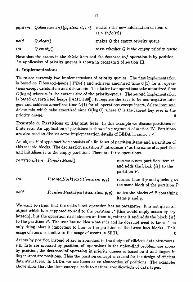
m-item Q.deerease_inf(pq_item it, I i)

void Q.clear 0

int Q.emptvO

makes i the new information of item it (i <_ i,~fo(it))

makes Q the empty priority queue

tests whether Q is the empty priority queue

Note that the access in the delete_item and the decrease_inf operation is by position. An application of priority queues is shown in program 2 of section III.

4. I m p l e m e n t a t i o n s

There are currently two implementations of priority queues. The first implementation is based on Fibonacci-heaps ([FT84]) and achieves amortized time O(1) for all opera- tions except delete_item and delete_min. The latter two operations take amortized time O(log n) where n is the current size of the priority-queue. The second implementation is based on restricted heaps ([AMOT88]). It requires the keys to be non-negative inte- gers and achieves amortized time O(1) for all operations except insert, delete_item and delete_rain which take amortized time O(log C) where C is the largest key ever in the priority queue. !

E x a m p l e 3, P a r t i t i o n s or Dis jo in t Sets: In this example we discuss partitions of finite sets. An application of partitions is shown in program 4 of section IV. Partitions are also used to discuss some implementation details of LEDA in section V.

An object P of type partition consists of a finite set of partition_items and a partition of this set into blocks. The declaration partition P introduces P as the name of a partition and initializes it to the empty partition. There are three operations.

partition_item P.make_block 0 returns a new partition_item it and adds the block {it} to the partition P.

int P.same_bloek(partition_item p, q) returns t r u e if p and q belong to the same block of the partition P.

void P.union_bloeks(partition_item p, q) unites the blocks of P containing items p and q.

We want to stress that the make_block-operation has no parameter. It is not given an object which it is supposed to add to the partition P (this would imply access by key lateron), but the operation itself chooses an item it, returns it and adds the block {it} to the partition P. The user has no idea what it is and he does not need to know. The only thing, that is important to him, is the partition of the items into blocks. This usage of items is similar to the usage of atoms in SETL. !

Access by position instead of key is abundant in the design of efficient data structures; e.g. lists are accessed by position, all operations in the union-find problem use access by position, the decrease-inf operation in priority queues is based on it and fingers in finger trees are positions. Thus the position concept is crucial for the design of efficient data structures. In LEDA we use items as an abstraction of positions. The examples above show that the item concept leads to natural specifications of data types.

94

III . G r a p h s

Graph algorithms are a prime example of combinatorial computing. We use the shortest path and the minimum spanning tree problem to illustrate LEDA's comfortable data type graph and its interaction with other data types. Program 2 shows Dijkstra's algorithm (cf. [AHU83], [M84,section IV.7.2], [T83]) for the single source shortest path problem in digraphs with non-negative edge costs.

(1) #include <LEDA/graph.h> (2) #include <LEDA/prio.h> (3) declare2 (priority_queue,node,float) (4) declare (node_array, pq_item) (5) void DIJKSTRA(graph& G, node s, edge_array(float)& cost, (6) node_array(float)& dis t , node_array(edge)& w e d ) (7) { priority_queue(node,float) PQ;

(8) node_array(pqJtem) I (G , nil); (9) pq_item it; (10) float c; (11) node u,v; (12) edge e; (13) forall_nodes (v, G) (14) { pred[v] = 0; (15) gist[v] = i n f i n i t y ; (16) I[v] = PQ.insert (v ,dis t[v]); (17) } (18) dist[s] = 0; (19) PQ.decrease_inf(I[s], 0); (20) while (!PQ.emptyO) (21) { it = PQ.delete_min0) (22) u = PQ.key( i t ) ; (23 ) forall_adj_edges (e, u) (24) { ~ = targa(e); (25) c = d i ~ t [ ~ ] + co~t[~]; (26) if ( e < dist[v]) (27) { dist[v] = c; (28) pred[v] = e; ( 2 9 ) PQ.decrease_inf(I[v], c); (30) } (31) } (32) } / /while (33) }

Program 2: Dijkstra's algorithm Program 2

95

The algorithm uses the data type graph and priority queue (lines (1) and (2)). The input to the algorithm is a graph G, a node s of G and a non-negative cost for each edge. It returns for each node v the length of a shortest path from s to v (array dist) and the last edge on such a shortest path (array pred). In LEDA we use edge- and node-arrays for the latter three parameters. A node_array(XYZ) is an array which is indexed by the nodes of some graph and whose entries have values of type XYZ. Thus a node_array(edge) is a mapping from node to edges.

The algorithm maintains for each node v a temporary distance label dist[v]. Ini- tially, dist[s] = 0 and dist[v] = co for v ¢ s, cf. lines (13)-(19). In LEDA the loop foraU_nodes(v, G)( . . . ) can be used to iterate over all nodes v of a graph G.

Dijkstra's algorithm uses a priority queue PQ. The priority queue contains pairs (v,dist[v]) and hence has type priority_queue(node, float); cf. lines (3) and (7). Each node v of the graph needs to know the position of the item < v, dist[v] > in the pri- ority queue. We therefore declare the data type node_array(pq_item) in line (4) and declare node_array(pq_item) I(G, nil) in line (8). In this declaration the parameter G tells LEDA that we want an array which is indexed by the nodes of G and the second parameter tells it tha t we want all entries initialized to the pq_item nil.

Initially, the items < s ,0 > and < v, i n f i n i t y > for v ~ s are put into PQ, cf. |ine (16). Then in each iteration we select and delete an item it with minimal i n f from PQ, cf. line (21). Let it = < u, dist[u] >, cf. line (22). We now iterate through all edges e start ing in edge u; cf. line (23). Let e = (u,v) and let c = dist[u] + cost[e] be the cost of reaching v through edge e, cf. lines (24) and (25). If c is smaller than the temporary distance label dist[v] of v then we change dist[v] to c and record e as the new predecessor of v and decrease the information associated with v in the priority queue., cf. lines (26) to (29).

The running time of this algorithm for a graph G with n nodes and m edges is O(n + m + Tdeclare + n(Tinsert + TDeletemin + Taet_inl) + m . TDecrease_~ey) where Tdedare is the cost of declaring a priority queue and T x y z is the cost of operation X Y Z . With the time bounds stated in section II we obtain an O(m + n log n) and O(m + n log C) algorithm respectively.

Program 2 is very similar to the way Dijkstra's algorithm is presented in textbooks, cf. [AHU83], [M84], [T83]. The main difference is that p r o g r a m 2 is e x e c u t a b l e c o d e whilst the textbooks still require the reader to fill in (non-trivial) details.

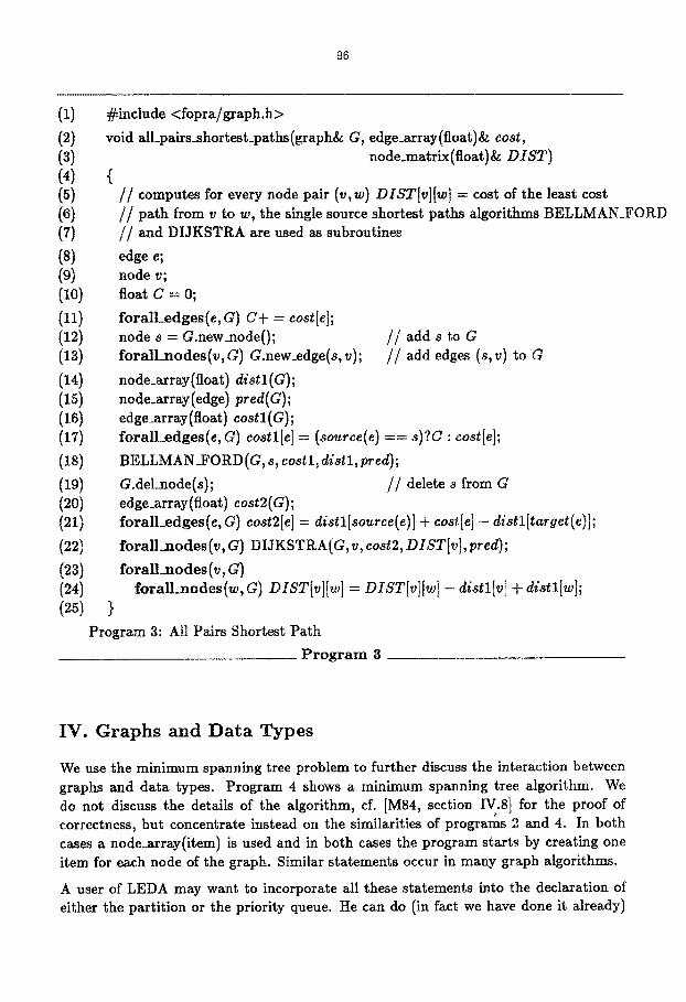
Dijkstra's algorithm is a useful subroutine for the solution of the all-pair shortest path problem in graphs with arbitrary edge costs, cf. [M84, section IV.7.4]. One uses the algorithm of Bellman-Ford to solve the single-source shortest path for some source s, then uses the solution of this computat ion to make all edge costs non-negative and then uses Dijkstra's algorithm to solve n - 1 single-source problems with non-negative edge costs. In order for this approach to work it is important tha t all nodes of the graph are reachable from s. The easiest way to achieve this is to add a new node s and to add edges of high cost from s to all other nodes. The details are given in program 3.

96

(1) #include <fopra/graph.h>

(2) void all_pairs_shortest_paths(graph& G, edge_array(float)& cost, (3) node.matrix(float)& DIST) (4) { (5) / / c o m p u t e s for every node pair (v,w) DIST[v][w] = cost of the least cost (6) / / p a t h from v to w, the single source shortest paths algorithms BELLMAN_FORD (7) / / a n d DIJKSTRA are used as subroutines

(8) edge e; (9) node v; (10) float C = 0;

(11) forall_edges(c,G) C+ = cost[e]; (12) node 8 = G.new_node0; / / a d d s to G (13) foral l_nodes(v,G) G.new_edge(s,v); / / a d d edges (s,v) to G

(14) node_array(float) distl(a); (15) node_array(edge) pred(G); (16) edge_array(float) costl(G); (17) forall. .edges(c, G) costl[e] = (source(e) == s )?C: cost[e]; (18) BELLMAN_FORD(G, s, costl, distl, pred); (19) G.del_node(s); / / d e l e t e s from G (20) edge_array(float) costZ(a); (21) forall_edges(e, G) cost2[c] = distl[source(c)] + cost[e] - distl[target(e)];

(22) fora l l_nodes (v, G) DIJKSTRA (G, v, cost2, DIST[v], pred); (23) foran_ odes(,, G) (24) foral l_nodes(w, G) DIST[v][w] = DIST[v][w] - distl[v] + distl[w]; (2s) }

Program 3: All Pairs Shortest Path

P r o g r a m 3

IV. Graphs and Data Types

We use the minimum spanning tree problem to further discuss the interaction between graphs and data types. Program 4 shows a minimum spanning tree algorithm. We do not discuss the details of the algorithm, cf. [M84~ section IV.8] for the proof of correctness, but concentrate instead on the similarities of programs 2 and 4. In both cases a node_array(item) is used and in both cases the program starts by creating one item for each node of the graph. Similar statements occur in many graph algorithms.

A user of LEDA may want to incorporate all these statements into the declaration of either the partition or the priority queue. He can do (in fact we have done it already)

97

(1) #include <LEDA/graph.h> (2) ~include <LEDA/parti t ion.h>

(3) declare (node_array,partition_item); (4) int cmp(edge el, edge e2, edge_float(array)& C) { return (C[e l ] - (C[e2]); }

(5) void MST(graph& G, edge_array(float)& cost, edgelist& EL) (6) / / t h e input is an undirected graph G together with a cost function (7) //cost on the edges; the algorithm outputs the list of edges EL of (8) / / a minimum spanning tree (9) { (10) node v, w; (11) edge e; (12) partition P; (13) node_array(partition_item) I(G); (14) forall_nodesCv, G) I[v] = P.make_block0;

(15) edgelist OEL = G.all_edges0; (16) OEL.sort(cmp, cost); (17) / /OEL is now the list of edges of G ordered by increasing cost

(18) EL.clear0; (19) forall(e, OEL) (20) { = sourceCe); (21) = targetCe); (22) if (!(P.same_block(I[v], I[w]))) (23) { P.union_blocks(I[v],I[w]); (24) EL.append(e); (25) ) (28) } (27) }

Program 4: Minimum Spanning Tree

P r o g r a m 4

so by deriving a data type node_partition from the data type partition (and similarly for priority_queue). A node_partition Q consists of a node_array(partition_item) I and a partition P. The declaration

node_partition Q( G) will then execute lines (3), (12), (13), and (14). The operations on node_partitions are also easily derived, e.g.Q.same_block(v,w) just calls P.same_block(I[v],I[w]). Alto- gether, this yields the simplified program 5.

The reader may ask at this point why we provide the elegant types node_partition and node_priority_queue in this roundabout way. Why do we first introduce items and then show how to hide them? The reason is that in the case of graphs the ground set of the partition or priority queue is static. In general, this is not the case

Consider for example, the standard plane sweep algorithm (cf. [M84, section VII.4.1,

98

(1) ~include <LEDA/graph.h> (2) #include <LEDA/partition.h>

(3) int crop(edge el, edge e2, edge_array(float)& C) { return (C[e l ] - (C[e2]); }

(4) void MST(graph& G, edge_array(float)& cost, edgelist& EL) (5) { node v, w; (6) edge e; (7) node_partition Q (G);

(8) edgelist OEL = G.all_edges0; (9) OEL.sort (crop, cost); (10) EL.clear0; (11) forall(c, OEL) 02) { ,., = sou,eeCe); (13) w = targetCe); (14) if (!(q.same_blockCv, w)) (15) { Q.union_blocks(v, w); (16) EL.append(e); 07) } ( is) } (19) }

Program 5: Simplified MST Program

P r o g r a m 5

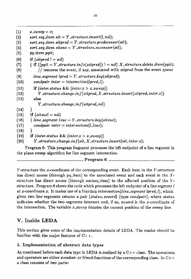
section VII.4.1]) for computing line segment intersections. It uses two information struc- tures, usually called the X- and Y-structure. The Y-structure is an ordered sequence of intersections of the sweep line with the line segments and the X-structure is a priority queue. The priority queue contains an event for each line segment l of the Y-structure which intersects the succeeding line segment lsuc in front of the sweep line. The event occurs when the sweep line passes the intersection.

In the algorithm the sweep line is moved from left to right. The sweep line stops whenever it passes through a left or right endpoint of a tine segment or through an intersection. In either case the X- and the Y-structure have to be updated appropriately. Consider for example the situation where a left endpoint of some line segment l is encountered at coordinate x. The following actions have to be taken: insert l into the Y-structure, say between Ipred and lsuc, remove the event, if any, associated with Ipred from the X-structure and add the events associated with lpred and l, if they exist.

The appropriate LEDA types are

sort_seq(line_segment ,pq_item) Y_structure;

priority_queue (sortseq_item,float) X_structure;

The Y-structure is a sequence of sortseq_items. Each item contains a line segment as its key and a pq_item as its information. The ordering is induced by the intersection of the line segments with the sweep line. Similarly, the X-structure stores for each item of the

99

(1) x_sweep = x; (2) sort_sea_item sit = Y_structure.insert (l, nil); (3) 8oct_sea_item sitpred = Y_structure.predecessor(sit); (4) sort_sea_item sitsuc = Y_structure.successor(Mt); (5) pq_item pait;

(6) if (s i tpred ! = nil) (7) { if ((pqi t = Y_structure.info(sitpred)) [= nil) X_strueture.delete_aem(pqit); (8) / / r emoves the event, if any, associated with sitpred from the event queue

(9) line_segment lpred = Y_strueture.key(sitpred); (10) condpair inter = intersection(lpred, l);

(n) if ( inter .s tatus ~ ( i . t e r .x > x_sweep)) (12) Y_structure.ehange_inf(sitpred, X_structure.insert(sitpred, inter.x)) (13) else

Y_structure.ehange_in f ( sitpr ed, nil) (14) } 05) if (sitsuc! : nil) (16) { line_segment Isue = Y_strueture.key(sitsuc); (17) condpair inter = intersection(l, lsuc); (18) } (19) if (inter.status a a (inter.x > x_sweep)) (20) Y_strueture.change_inf(sit, X_structure.insert(sit, inter.x);

Program 6: This program fragment processes the left endpoint of a line segment in the plane sweep algorithm for line segment intersection.

P r o g r a m 6

Y-structure the x-coordinate of the corresponding event. Each item in the Y-structure has direct access (through pq_item) to the associated event and each event in the X- structure has direct access (through sortseqAtem) to the affected position of the Y- structure. Program 6 shows the code which processes the left endpoint of a line segment l at x-coordinate x. It makes use of a function intersection(line_segment lpred, l), which given two line segments returns a pair (status, xcoord) (type condpair), where status indicates whether the two segments intersect and, if so, xcoord is the x-coordinate of the intersection. The variable x_sweep denotes the current position of the sweep line.

V. Ins ide L E D A

This section gives some of the implementation details of LEDA. The reader should be familiar with the major features of C++.

1. I m p l e m e n t a t i o n of a b s t r a c t d a t a t y p e s

As mentioned before each data type in LEDA is realized by a C + + class. The operations and operators are either member- or friend-functions of the corresponding class. In C + + a class consists of two parts:

100

a) The declaration of the class describes the interfaces of its member functions (return and parameter types). This part of a class corresponds to the abstract specification of the data type. As an example we give the declaration of the class partition (used in programs 4 and 5):

int void void

partition() partition()

};

/ / a partition is a forest of partition_nodes

class partition_node {

fr iend class partition;

/ /pr ivate:

partition_node, f a the r ; / /pa ren t node in the forest partition_node* next; / / t o link all used nodes int size;

public:

partition_node(partition_node* n) { father=0; size=l; next=n~ }

}

/ / a partition item is a pointer to a partition node;

t ypede f partition_node* partition_item;

class partition {

//private: partition_item used_items; / / l i s t of used partition items

public: / /operat ions

partition_item make_block(); partition_item find_block (partition_item);

same_block (par tition_item, partition_item); union_blocks (partition_item, partition_item); clear();

{ used_items = 0; } / / cons t ruc to r { clear(); } / /des t ructor

Only the public part of class partition appears in the LEDA manual.

b) The implementation of the class is the C + + code realizing the member functions declared in part a). The implementation of class partition follows:

/ / u n i o n find with weighted union rule and path compression

partition_item partition::make_block 0 { / / c r ea t e new item and insert it into list of used item

used_items = new partition_node(used_items); r e t u r n used_items;

}

t01

partition_item partifion::find_block(partition_item it) { / / r e t u r n the root of the tree that contains item it

partition_item x,root = it;

whi le (root--*father) root = root-~father;

/ / p a t h compression:

whi le (it!=root) { x = it--~father;

it---~father = root; it = x;

} r e t u r n root;

}

int partition::same_block(parfition_item a, partit ionJtem b) { r e t u r n find_block(a)==find_btock(b); }

void partition::union_blocks(partition_item a, partition_item b) { / / w e i g h t e d union

a = find_block(a); b = find_block(b);

if(a-*size > b--~size) { b-+father = a;

a--~size + = b--+size; } else{ a--~father = b;

b-~size + = a--~size; }

}

void partition::clear 0 { / / d e l e t e all used items

partition_item p = used_items; whi le (used_items) { p = used_items;

used_items = used_items--mext; dele te p;

} }

Note that only member functions or member functions of friends are allowed to access the private data of a class. This guarantees that the user of a class can manipulate objects of this class only by using member functions, i.e. only by the operations defined in the specification of the data type. This data hiding feature of C + + supports complete separation of the specification and the implementation of data types.

For every data type XYZ there exists a so-called header file "XYZ.h" containing the declaration of class XYZ. Programs using XYZ have to include this file. For example, partitions can only be used after the line

102

~include <LEDA/partition.h> (see program 4)

The implementation of all classes are precompiled and contained in a module library which can be used by the linker.

2. P a r a m e t r i z e d Types

Most of the data types in LEDA have type parameters. In section II we defined a dictionary to be a mapping from a key type K to an information type I, here K and I are formal type parameters. The LEDA statement

"declare2 (dic t ionary , t l , t2 )"

declares a dictionary type with name "d ie t ionary ( t i , t2)" and actual type parameters K = tl and I = t2. How is this realized?

Note that the operations on a dictionary are independent of key type K and information type I. So it is possible to implement all dictionary operations (member functions) without knowing K and I. This is done by implementing a base class dictionary with K = I = void*. For example

class dictionary { / / b a s e class

/ /p r iva te data

public:

void insert(void* k, void* i);

void* access(void* k);

};

In C++ the type void* (pointer to void) is used for passing arguments to functions that are not allowed to make any assumptions about the type of their arguments and for returning untyped results from functions. To declare a concrete data type for given actual type parameters (e.g., dictionary(int,int)) a derived class of the corresponding base class (dictionary) has to be declared. This derived class inherits all operations and operators from its base class and performs in addition all necessary type conversion:

class dictionary(int,int): public dictionary {

void insert(int k,int i) { dictionary::insert((void*)k, (void*)i); }

int access(int k) { return (int)dictionary::access((void*)k); }

};

103

C+÷ ' s macro facility is used to fill in such declarations of derived classes. There are macros declare, declare2, . . . to declare data types with one, two, . . . type parame- ters. dectare2(dictionary, int,int) for example just creates the above declaration of dic- tionary(int,int).

3. I t e r a t i o n

LEDA provides various kinds of iteration statements. Examples are

for lists:

forall(x, L) { the elements of L are successively assigned to x}

for graphs:

forall_nodes(v, G) { the nodes of G are successively assined to v}

forall_adj_nodes(w, v) { the neighbor nodes of v are successively assigned to w}

All these statements are macros that are expanded to more complicated for-statements. The list iteration macro forall is defined as follows

~define forall(x,L) for(L.init_cursor0; x = L.current_element0; L.move_cursor0; )

Here init_cursor0, move_cursor 0 and current_element 0 are member functions of the class list that manipulate an internal cursor.

The other iteration statements are implemented similarly.

VI. Experiences

We report on our experiences in designing, implementing and using LEDA.

We found the task of specifying a data type surprisingly difficult. The data types dictionary and priority queue were the first two examples which we tried. The dictionary was readily specified; we had, however, lengthy discussions whether a dictionary is a function from keys to variables of type I or to objects of type I. The former alternative allows array notation for dictionaries, e.g. line 8 in program 1 could be written D[k] + +, but also allows the user to store pointers to variables in our modules. The latter alternative makes notation more cumbersome but seems to be safer. We did not resolve the conflict but now have both alternatives to gain further insight by experiments. The priority queue took us a long time. We wanted to support access by position and we wanted a complete separation of data type and data structure. We found neither the combinatorial algorithms nor the abstract data type literature very helpful. In the algorithms literature the position concept is usually only discussed in the context of concrete implementations and is then equated with an index in an array or a pointer to a node of a data structure. In this way, no abstract definition of the data type is given and the data structures are intimately tied with the applications; e.g. priority queues are tied to shortest path calculations and partitions are tied to graph algorithms. In the latter part of the literature the position concept is only discussed in simple examples, e.g. iterators in linear lists [TRE88].

104

We use items as an abstraction of positions. Items are similar to the atoms of SETL. We found the item approach very flexible and, once we used it for priority queues, the specification of data types like sequences, partitions and lists became easy.

The implementation of LEDA was mostly done by the second author, in particular, lists, graphs, and sorted sequences were implemented by him. Once the standards were set, we asked students to join in and to either realize additional data types or to give alternative realizations. Implementations of various kinds of dictionaries (BB[a]-trees, red-black- trees, (a,b)-trees, dynamic perfect hashing) and priority-queues (Fibonacci-heaps, C- heaps) were provided by Dirk Basenach, Jfirgen Dedorath, Evelyn Haak, Michael Muth, Michael Wenzel and Walter Zimmer.

LEDA was used to write graph and geometry algorithms. Some examples are shortest paths, components of various kinds, unweighted and weighted matchings, network flows, embeddings of planar graphs, visibility graphs of line segments, Voronoi diagrams and intersection of half spaces. The graph users liked LEDA because all the required data types such as graphs, node- and edge-arrays, lists, dictionaries, . . . were available and hence LEDA increased their productivity enormously. This has led to more experimental work, one of the goals of the project. The first geometry users of LEDA were much less enthusiastic because almost none of the required types such as points, lines, . . . were available. Stefan Meiser implemented some of them and we are now hearing the first positive reactions from the geometry users.

VII. Conclus ions

LEDA is a library of efficient data types and algorithms. At present, its strength is graph algorithms and the data structures related to them. The computational geometry part is evolving.

There are several other projects which aim for similar goals as LEDA, e.g. [B88, So89, L89]. We believe, that LEDA compares well with these systems because of the

- clear separations between specification and implementation,

- the natural syntax, and

- the inclusion of many of the most recent and most efficient data structures and algorithms.

We close this section with a list of algorithms that we implemented using LEDA data types. All graph algorithms are part of the library. A LEDA function F(graph& G,...) accepts any user-defined graph type (graph(node_type, edge_type)) as argument.

1. G r a p h Algo r i t hms

1.1. Basic Graph Algorithms

- depth first search

- breadth first search

105

- connected components

- transitive closure

1.2. Shortest Path Algorithms (see section III)

- Dijkstra's algorithm

- Bellman/Ford algorithm

- all pairs shortest paths

1.3. Matchings

- maximum cardinality bipartite matching

- maximum weight bipartite matching

1.4. Network Flow

- maximum flow algorithm of Galil/Namaad

- maximum flow algorithm of Tarjan/Goldberg

1.5. Planar Graphs

- triangulation

- straight line embedding

2. Computa t iona l Geomet ry

- intersection of half spaces

- convex hull of point sets

- construction of Voronoi diagrams

- construction of visibility graphs

Acknowledgement: We want to thank our colleagues G. Hotz, J. Loeckx, K. Sieber and R. Wilhelm for many helpful discussions.

V I I I , R e f e r e n c e s

[AMOT88]

[AHtTS ]

[B88J [BKMRS84]

R.K. Ahuja, K. Mehlhorn, J.B. Orlin, R.E. Tarjan: ~'Faster Algorithms for the Shortest Path Problem", Technical Report No. 193, MIT, Cam- bridge, 1988

A.V. Aho, J.E. Hopcroft, J.D. Ullman: "Data Structures and Algo- rithms', Addison-Wesley Publishing Company, 1983

A. Bachem: Personal Communication, 1988

A. Mfiller-von Brochowski, T. Kretschmer, J. Messerschmitt, M. Ries, J. Sch/itz : "The Programming Language Comskee", Linguistische Ar- beiten, Heft 10, SFB 100, Univ. des Saarlandes, Saarbrficken, 1984

106

[FT84]

[L89]

[M84]

[SoSg] [St86]

[T83]

[TRE88]

M.L. Fredman, and R.E. Tarjan: "Fibonacci Heaps and Their Uses in Improved Network Optimization Algorithms", 25th Annual IEEE Syrup. on Found. of Comp. Sci., 338-346, 1984

C. Lins: "The Modula-2 Software Component Library", Springer Pub- lishing Company, 1989

K. Mehlhorn: "Data Structures and Algorithms", Vol. 1-3, Springer Publishing Company, 1984

J. Soukup: '+Organized C", Typescript, 1988

B+ Stroustrup: " The C++ Programming Language", Addison-Wesley Publishing Company, 1986

R.E. Tarjan: "Data Structures and Network Algorithms", CBMS-NSF Regional Conference Series in Applied Mathematics, Vol. 44, 1983

P. Thomas, H. Robinson, J.Emms: '+Abstract Data Types", Oxford Applied Mathematics and Computing Science Series, 1988