DEPARTMENT OF STATISTICS

University of Wisconsin

1300 University Avenue

Madison, WI 53706

TECHNICAL REPORT NO. 1143

July 10, 2008

A Linear Mixed Effects Clustering Model for Multi-species Time

Course Gene Expression Data1

Kevin H. Eng

Department of Statistics

University of Wisconsin, Madison

Sunduz Keles

Department of Statistics

Department of Biostatistics and Medical Informatics

University of Wisconsin, Madison

Grace Wahba

Department of Statistics

Department of Biostatistics and Medical Informatics

University of Wisconsin, Madison

1This work was supported by NSF grant DMS-0604572 (GW), ONR N0014-06-0095 (GW), a PhRMA

Foundation Research Starter Grant (SK) and NIH grants HG03747-01 (SK) and EY09946 (GW)

Abstract

Environmental and evolutionary biologists have recently benefitedfrom advances in experimental design and statistical analysis for com-plex gene expression microarray experiments. The high-throughputtime course experiment highlights gene function by uncovering func-tionally similar responses across varied experimental conditions. Sincethese time-dependent responses can be compared across phylogeneticbranches, we argue that the extension to multi-factor designs incor-porating closely related species adds an evolutionary context to theanalysis as well as being of considerable interest in its own right. Mo-tivated by time course gene expression experiments conducted overmultiple strains of yeast, we propose a mixed effects model basedclustering method that preserves the factor information contained intime and in species. The result is a partitioning of the common, ho-mologous genome into functional groupings cross-tabulated by theirresponse in different species and annotated by their mean effects anddependence in time and over phylogeny. In a set of experiments con-taining yeast species in the Saccharomyces sensu stricto complex, wegive examples of detectable patterns and describe inferences of intereston their estimated covariances. We demonstrate via simulation that amixed effects type model has good clustering properties and is robustto noise.

Keywords: Comparative biology; Cluster analysis; Gene expres-sion; Linear mixed models; Microarrays; Mixture models; Time coursegene expression.

1

A Linear Mixed Effects Clustering Model forMulti-species Time Course Gene Expression

Data

Kevin H. Eng, Sunduz Keles∗, and Grace WahbaDepartment of Statistics,

Department of Biostatistics and Medical informatics,University of Wisconsin-Madison,

1300 University Ave., Madison, WI 53706, USA.*keles@stat.wisc.edu

July 10, 2008

1 Introduction

Understanding the mechanisms behind the evolution of gene function is amajor challenge in evolutionary biology. While biologists have traditionallystudied genes’ biochemical and structural functions based on the variationsin coding sequences, many studies have argued and demonstrated that agene’s function can also be defined by its role in specific cells, tissues, organs,genetic pathways and whole organisms. The study of gene expression traitsconnects these higher order phenotypes to the information contained in thegenome. With the advent of microarray technology, it is possible to measureand identify expression differences within and among species across wholegenomes (Rifkin et al., 2003; Fay et al., 2004; Khaitovich et al., 2004; Giladet al., 2006; Whitehead and Crawford, 2006).

Variations in expression have been long recognized as a fundamental partof the process of evolution (Britten and Davidson, 1969; King and Wilson,1975; Wray et al., 2003); King and Wilson (1975) argued 30 years ago thatdifferences in gene regulation may be responsible for differences between

2

closely related species. Naturally, early cross-species microarray studies in-vestigated differences unexplainable by DNA coding sequence, measuringexpression under various experimental conditions. Gilad et al. (2006), forexample, compared gene expression in liver tissue within and between hu-mans, chimpanzees, orangutans and rhesus macaques and, consistent withKing and Wilson’s hypothesis, identified of a set of human-specific genesencoding transcription factors, DNA binding proteins.

With the maturation of microarray technology, comparative experimentsare increasingly common, leading evolutionary biologists to a curious sort ofinduction: instead of single genes they must contend with information fromentire genomes. Aggregating expression over different Drosophila lines, Rifkinet al. (2003) argue that the percentage of genes showing expression divergenceis a useful measure of evolutionary distance versus the divergence in sequenceof a few select genes. Whitehead and Crawford (2006) state that the effects ofbalancing selection are easily identified in different populations of Fundulusheteroclitus since the microarrays simultaneously measure a sufficient numberof genes to provide a proper estimate of gene-wise variation.

The result is the ability to consider evolutionary hypotheses at the levelof single genes distinguished from thousands of patterns across the wholeorganism. The previous two studies, as well as Khaitovich et al. (2004) andNuzhdin et al. (2004), are particularly interested in testing Kimura’s (1991)neutral drift (neutral evolution) hypothesis on each gene, which states thatthe correlation in a particular trait between species is inversely proportionalto the phylogenetic distance between them. This neutral evolution theoryimplies a particular structure (a phylogenetic tree), and, for multivariate nor-mal traits, it can be argued that the signature of evolution may be observedin a tree-structured covariance matrix (Gu, 2004; McCullagh, 2006).

All of these studies involve a small number of species measured over onlya few experimental conditions and are therefore conveniently analyzed withwell established statistical tools (Kerr and Churchill, 2001; Smyth et al.,2003). A common extension of single condition experiments is to profileexpression over a time course (Chu et al., 1998; Bar-Joseph et al., 2002; Luanand Li, 2003; Storey et al., 2005; Yuan and Kendziorski, 2006; Qin and Self,2006; Tai and Speed, 2006). While conventional gene expression analysis canassociate individual genes with a single condition (e.g., tissue type or habitattemperature), a time course gene expression analysis ties genes together intofunctional groups and prompts their association with underlying biologicalprocesses. Such processes can be natural cycles (Spellman et al., 1998), or

3

they can be a response to a stimulus as in the yeast Environmental StressResponse (Gasch et al., 2000).

In these analyses, the assumption is that genes which are correlated withone another are likely represent functional groups and the goal is to uncoverthese biological clusters. Among the clustering models for time course geneexpression data, model based clustering (Fraley and Raftery, 2002) is widelyused because it provides a flexible and adaptive alternative to nonparamet-ric/algorithmic clustering techniques (k-means or hierarchical clustering). Inparticular, the regression clustering models in Qin and Self (2006) use thetime factor to model the observed signal leading to interpretable regressioncoefficients and variances and to facilitate formal hypothesis testing. In par-ticular, with the incorporation of random effects terms (Luan and Li, 2003;Ng et al., 2003; Qin and Self, 2006) these models can accommodate higherlevels of heterogeneity among expression profiles of individual genes and caninduce correlations among expression levels across different time points.

Although, the literature of well-studied statistical models for single speciesexperiments is considerable, their multi-species counterparts have not fullyemerged. Ideally, new models incorporating species components to gene ex-pression studies will admit the analyses we highlighted above: tests of naturalselection hypotheses versus neutral drift and the ability to study gene specificphylogenies, “gene trees,” in detail. In this article, we develop a frameworkfor analyzing multi-species time course gene expression experiments basedon a comparative (i.e., across species) linear mixed effects clustering model.Our proposed approach produces significant gains over existing methods bycarefully balancing the functional implications of the time factor with theevolutionary implications of the species factor. We compare and contrastmodel based clustering and regression clustering models which differ basedon their parameterizations of the mean expression profiles across the timecourse and across strains. We discuss fitting issues, conduct simulation stud-ies comparing the relative performances of other clustering models on thistype of data, and give the results of an analysis on a multi-species yeast heatshock stress response data set.

4

2 Methods

2.1 Clustering Model

In the time course gene expression experiment, it is of interest to groupgenes together by their common structure over time since genes with similartime profiles may have similar biological functions. A naive approach isto model each gene with its own linear model and to test or cluster thecoefficients into similar patterns. Instead of a model for every gene, Qin andSelf’s class of clustering of regression models (2006) assumes that every genemeasured belongs to a class defined by a linear mixed effects model with arandom effect for time. Genes in the same class share the same mean timeprofiles and the same longitudinal dependence structures. The net effect isa more parsimonious representation of the experiment and a greater numberof observations (entire genes) available for estimation. We intend to extendthis model to incorporate an additional random effect for species.

In the multi-species time course experiment, we measure gene expressions,Ygsti, for observation i = 1, . . . , N of species s = 1, . . . , S at time t = 1, . . . , Tfor each gene g = 1, . . . , G. For simplicity, we assume that each species ismeasured on the same set of time points, that the species are sufficientlysimilar to allow us to measure a set of comparable orthologs. Then, obser-vations for each gene are contained in Yg ∈ RSTN×1. The naive approachmodels each of these vectors individually with a per-gene linear mixed effectsmodel,

Yg = Xβg +Wag +Mbg + εg, (1)

where βg ∈ RTS×1 are gene specific fixed effects, ag ∈ RT×1 are random effectsin time and bg ∈ RS×1 are random effects across species with appropriatedesign matrices X, W , M . While this model assumes that each gene hasits own mean and covariance, the assumption is often impractical becausethe number of observations of any single gene are few and it is of interest toexploit common structures between functionally similar genes.

We choose, therefore to follow Qin and Self (2006) and to designate k =1, . . . , K component models. For gene g, let Ug ∈ {1, . . . , K} be the clusteringvariable. The model for a complete vector, Yg, in cluster k, is given by:

Yg | {Ug = k} = Xβk +Wagk +Mbgk + εgk, (2)

where the fixed effects (βk) and random effects (agk and bgk) are now cluster

5

specific. That is, we assume that

agk = ag | {Ug = k} ∼ N (0, Ak),

bgk = bg | {Ug = k} ∼ N (0, Bk), (3)

εgk = εg | {Ug = k} ∼ N (0, σ2kI),

are conditionally independent multivariate normal random variables wherethe covariance matrices Ak are of dimension T × T and Bk are S × S, bothof unspecified structure. Under these assumptions, a gene from cluster k hasthe following marginal distribution:

Yg | {Ug = k} ∼ N (Xβk, Vgk) , (4)

Vgk = WAkW′ +MBkM

′ + σ2kI. (5)

In this model, the cluster centers are the regression coefficients, βk, or equiv-alently the mean time profiles over all species, Xβk. This means that genesshowing common species specific differences (as well as common time pat-terns) will tend to group together into the same cluster. Then, each compo-nent represents a unique functional pattern and instead of describing eachgene as a mixture, the model tries to assign the gene to a single cluster. Inpractice, goodness of fit can be assessed by considering the clustering cer-tainty, hopefully each gene is ascribed to only one cluster with high posteriorprobability.

Our model can be reduced to other mixed effects clustering models withspecies components such as Ng et al. (2003), who propose a multiple ran-dom effects model but use only diagonal covariances. In a data set wherethere are many time points, it may be fruitful to consider spline modelsover time, as in Luan and Li (2003), who use B-spline bases to model bothfixed and random effects for time course data. In a paper to appear shortly,Ma and Zhong (2008) propose a functional (a.k.a smoothing spline) ANOVAmodel with smoothing splines for time course cluster means and random ef-fects covariates which could model a species factor, treated as part of theloss function. In the sense that model based clustering (Mclust) (Fraley andRaftery, 2002) parameterizes the variance of a gaussian component throughthe eigenvector decomposition, clustering of regression models (Qin and Self,2006) parameterize both the mean and variance. Our clustering of mixedeffects models further parameterizes the variance terms taking advantage ofthe covariate information. These regression models can be less parsimoniousthan the simplest Mclust models but they add parameters which are of par-ticular interest.

6

2.2 Structured Covariances

Using two random effects separates correlation attributable to time pointsAk from correlation between species Bk. In this article, we assume onlythat these matrices are positive definite, but the model may be adapted forany structured form. For example, if we wish to impose an autoregressivescheme in time we may use the formulation in McCulloch and Searle (2001)(pp. 193, 201) for Ak and derive an estimating equation for the autoregressiveparameters. Generally, the matrix Bk is a representation of the branchingstructure of a Brownian motion diffusion process describing an evolutionaryhistory (Felsenstein, 1973), and the estimation we describe admits two typesof analysis important to evolutionary biology.

In phylogenetic analyses, the tree-structured form of Bk (McCullagh,2006) is of interest and predicted random effects E(bgk|Yg, Ug) represent cor-rections to expression due to the species factor (phylogeny). Corrada Bravoet al. (2008) argue that estimating Bk under tree-structured constraints ad-mits a gene expression derived phylogenetic effect. The estimate may becompared against a sequence derived covariance in order to determine devi-ation from neutral drift. As a practical procedure, consider a predefined setof “pseudogenes” (Khaitovich et al., 2004), genes for which there ought tobe no force of selection. The covariance estimated on the set of psuedogenesmight be used as an estimate of the neutral drift covariance for hypothesistesting.

In comparative analyses, the matrix Bk is a nuisance parameter typicallyestimated from DNA sequence data. Freckleton et al. (2002) argue that theprimary interest in modeling this dependence is to make better inferencesabout βk, so it is not unreasonable to attempt to estimate Bk directly fromexpression data. Alternative models of note are the modeling procedure de-scribed in Guo et al. (2006) which chooses among 3 possible parameterizedversions of Bk to find a good correction for the observed phylogenetic de-pendence, and a similar formulation in Eng et al. (2008) which estimates amixing proportion to control a continuum of corrections.

2.3 Model Fitting

In a given experiment, we only observe Yg; therefore we treat Ug, agk, andbgk as missing data and apply the Expectation-Maximization (EM) algorithm(Dempster et al., 1977), described in Appendix A, to fit the model. Because

7

the EM algorithm is known to be sensitive to the choice of initial startingvalues (McLachlan and Krishnan, 1996), instead of a random initialization,we seed the model with a per-gene analysis, an exploratory clustering method“Mclust on coefficients” described in later sections.

Gene pre-screening. Since we are only interested in genes that show atleast some time dependent effect, we can pre-screen the genes by fitting afixed effects ANOVA model with time and species factors to each gene andthen removing genes with insignificant main effects for time. Pre-screeningon F-statistics admits some false discovery rate (FDR) control, but we notethat the assumption of a heterogeneous covariance structure is inconsistentwith the standard ANOVA application and we expect that the F-statisticsmay lose some control of the FDR. As we will demonstrate in the simulationsection, it turns out that making false positive errors here is not too dramaticsince the clustering model seems to be able to identify and isolate singletonnoise. Therefore, it is generally advisable to choose a pre-screening thresholdbased on the maximum number of genes of interest or based on a targetFDR somewhat larger than usual, and to test the time effect hypothesisafter clustering.

Choosing the number of clusters. It has been argued that using BIC(Schwarz, 1978) is appropriate to choose the number of components in a finitemixture even though mixtures violate the standard regularity conditions forlikelihood methods (Fraley and Raftery, 1998). Especially for models whichparameterize the variance, we find that BIC is too strict in that it favors asmall number of components in cases when graphical checks and biologicalinsight suggest otherwise (Eng et al., 2007). Suppose that pµ and pΣ arethe number of parameters associated with the mean and variance of a singlecomponent respectively and ll(K) = logL(θK ;Y |K) is the log likelihood fitfor K clusters. Then BIC(K) = −2ll(K) +K(log n)(pµ + pΣ) favors K + 1components over K when BIC(K + 1) < BIC(K) or

ll(K + 1)− ll(K) > (log n)(pµ + pΣ)/2, (6)

L(θK+1;Y |K + 1)

L(θK ;Y |K)> n(pµ+pΣ)/2. (7)

Here, we observe the convention in Fraley and Raftery (1998) of not addingthe mixing proportion to the set of free parameters. In order for a mixture tochoose K + 1 components versus K, the improvement in log likelihood mustovercome the penalty for all the parameters associated with a component’s

8

mean and variance. Thus, there is some tradeoff between the complexity inthe component level model (particularly the covariance) and the number ofcomponents. Recalling that this preference for simple models is a standardproperty of BIC, we would ideally want to enforce a parsimonious represen-tation in the number of components (K) that fairly penalizes componentmodel complexity (pµ and pΣ); we want a criterion that gives equal penaltyto simple covariances and to complex covariances.

In practice, models with too few clusters can be detected by inspectionsince clusters will appear too heterogeneous while models with too manyclusters might appear to have clusters which could be combined. Intuitively,if two components are similar but have different means, it may be less costlyto combine the two clusters inflating their single covariance. Qin and Self(2006) may have similarly observed this problem since they suggested a com-bination of BIC, for a good predictive fit, and the maximum of the boot-strapped largest eigenvalues of the cluster covariance matrices (the BMV -bootstrapped maximum volume), penalizing this over-dispersion.

A standard alternative to BIC might be to choose the number of clustersbased on cross validated likelihood; that is, we can choose the number ofcomponents in the mixture based on estimated out of sample predictionperformance. For a mixture, it is natural to use the negative log likelihoodas a loss function (van der Laan et al., 2004).

In the next section, we demonstrate the application of this model to a dataset with multiple species of yeast measuring their temporal response to heatshock. In later sections we will demonstrate that accounting for structuredheterogeneity in observations leads to better clustering results even in thepresence of large variances and un-clusterable, singleton noise.

3 Data Analysis

Tirosh et al. (2006) measured the response to heat shock in four species ofyeast on two-channel DNA microarrays by arraying a sample from each timepoint against a baseline measurement from the same culture. So, the logratio measurements represent a relative change due to stress over time. Forillustration of a complex interspecies design, we combine this data set with ananalogous heat shock experiment over 5 strains of Saccharomyces cerevisiaefrom the Gasch Lab at Wisconsin (Eng et al., 2008).

In total, there are 6 strains of S. cerevisiae (S288C, K9, M22, RM11a,

9

YPS163, BY4743), 2 strains of S. paradoxus (CBS432 and NRRL Y-17217)and one each of S. kudriavzevii and S. mikatae representing 4 closely relatedspecies. The strains are measured over 9 time points (5, 10, 15, 20, 30, 45, 60,90, 120 minutes post heat shock) with 110 total arrays (60 from the GaschLab and 50 from Tirosh et al. (2006)). We normalize within arrays, and quan-tile normalize arrays taken at the same time points. The normalization ofarrays across laboratories is a current research topic elsewhere (Consortium,2005) and not addressed further in this article.

[Figure 1 about here.]

Each study’s arrays measure over 5000 yeast genes of which 3542 geneshave orthologous sequences in every species. As described in Section 2.3,pre-screening the genes with a per-gene two way ANOVA model selects 2606genes with significant time patterns (FDR < 0.01).

[Table 1 about here.]

Using Mclust’s mixture of gaussians to cluster the log ratios directly yieldsa mixture of 48 components with the same diagonal covariance by BIC. Dueto the dimension of the data, Mclust can only search through its predefined“diagonal” and “spherical” covariance models (Fraley and Raftery, 2002). InTable 1, we list the best K for each of the available models. We only considerMclust models which add pµ mean and pΣ covariance parameters per cluster,omitting the models which share parameters across clusters. Note that forthese alternatives, K = 48 is the largest number of components estimable.

A first approximation of a clustering of regressions model may be fit byapplying Mclust to the coefficients of the per-gene ANOVA models. Sincethe coefficients represent a transformation of the data, this is a reasonableexploratory procedure (analogous to how Mclust uses hierarchical clusteringto choose its seed assignments, Eng et al. (2007)). It is somewhat more fairthan the vanilla Mclust since it only considers the covariance between groupmeans. BIC values from this model fit are not directly comparable to theother procedures. This procedure chooses K = 82 components which weuse as an upper limit for the number of clusters. Applying agglomerativeclustering to the cluster centers, for every K ≤ 82, we may seed the mixedeffects clustering model by assigning genes to clusters based on which clusterscollapse together for a particular K.

10

Table 1 includes BIC values for K = 5, the choice if we follow BICstrictly, and K = 12, the choice if we follow cross-validated likelihood (CV)which minimizes out of sample prediction error. Choices for K by the usualMclust procedure as well as the Mclust on coefficients procedure are alsotabulated. In all cases, the BIC criterion for the mixed effects model ismuch smaller than all of the Mclust models implying any one of the mixedeffects models is a better fit. This is, of course, not surprising since we usecovariate information to improve the model fit (pµ = 110 for Mclust modelswhile pµ = 18 for mixed effects models). The count of component specificparameters pµ and pΣ are included in the table to illustrate the magnitudeof the BIC penalty for adding a single component. It is not clear whichresult we should favor; by inspection we find K = 5, 12 too coarse (median524,298 genes per cluster) and even at K = 48 clusters are still relativelylarge (median x genes per cluster). For illustration, we present the resultsfor K = 82 (24 genes per cluster), chosen by Mclust on coefficients, later inthis section.

Beyond information criteria, a primary tool in evaluating the goodnessof the clustering model fit is a high resolution heat map plot. For plotscomparing a best Mclust fit, a comparable hierarchical clustering fit and aselection of linear mixed effects clustering model fits, see the SupplementaryFigures 1-6 online. We can also determine goodness of clustering by consid-ering a silhouette type plot (van der Laan and Bryan, 2001). Since one ofthe byproducts of the EM fit is a posterior probability of cluster membershipwe sort genes by their cluster assignment and their posterior probability ofbeing in that cluster. Supplementary Figure 7 shows that, for the mixedeffects clustering model, nearly all genes (2575 / 2606) have greater than 0.5posterior probability of being in their assigned class, a good clustering result.

More specifically, we may investigate interesting clusters through theirfitted time patterns. In Figure 1, we plot one cluster with a consistent timepattern representative of a single function. The 47 genes in this cluster arestrongly associated with Gene Ontology (GO) biological process “ubiquitin-dependent protein catabolic process” (GO:0006511, 26 of 113 genes present,p < 1×10−14); GO molecular function “endopeptidase activity” (GO:0004175,21 of 28 genes present, p < 1× 10−14); and several GO cellular components,particularly “20S core proteasome” (GO:0005839, 13 of 15 genes present, p <1×10−14) via geneontology.org, yeastgenome.org and funspec.med.utoronto.ca.Ubiquitin, endopeptidase and the 20S proteasome have well characterizedroles in the detection of damaged proteins and their degradation during cel-

11

lular stress. We might interpret this effect as a sudden increase, in responseto heat shock, in the production of genes which identify and eliminate dam-aged proteins followed by a rapid return to some new equilibrium state. Themagnitudes of the new equilibrium are different, in particular, the profilesshow a similar specific effect in the M22 strain of S. cerevisiae and the S.mikatae strain. We can hypothesize that both of these require a large (netpositive) increase in the resting expression of genes associated with this pro-cess. M22, for example, is known to grow poorly at 37C so a higher rate ofubiquitin production may be a compensatory mechanism. These 47 genes ap-pear together in the same cluster (along with other genes) for every K ≤ 82suggesting a reasonably consistent clustering result.

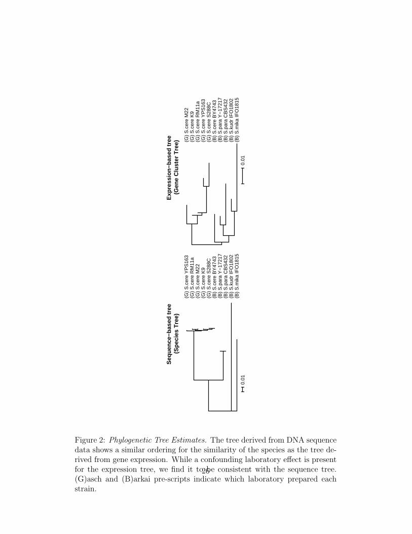
Further downstream analysis utilizes the attributable phylogenetic effect,the predicted random effects (bgk) of the species under study. We interpretthese as the component of the observed signal that can be attributed to theunderlying dependence due to species factors alone, independent of time.For the cluster of 47 genes above, we find the closest sum-absolute-valuenorm tree corresponding to the estimated covariance (Bk) (Corrada Bravoet al., 2008), building a gene expression based tree (Figure 2). The tree es-timate’s first split places 5 of 6 S. cerevisiae strains together, a reasonableresult (strains should be more similar than species), however the differenceis confounded by which lab prepared the assay. Labs are denoted (G) forGasch Lab and (B) for the Barkai lab from Tirosh et al. (2006). For compar-ison, Figure 2 also provides the sequence derived tree using DNA sequencefrom a sample of upstream coding regions of the strains in the study. SinceS. paradoxus CBS432 has not been sequenced, we place it along-side theother paradoxus strain. This estimate represents the species tree since itsamples from homologous sequences. Further, since it uses DNA sequenceinformation, it is not confounded with the laboratory effect. Trees estimatedfrom sequence and expression data play a role in the comparative analysisdescribed in Eng et al. (2008).

[Figure 2 about here.]

12

4 Simulation Studies

4.1 Candidate Models

In order to investigate the advantages of explicitly accounting for differentexperimental factors and their induced correlations, we consider two appli-cations of Mclust models (Fraley and Raftery, 2002) and two fixed effectsmodels. All of the methods are similar in that they model the marginaldistribution of a gene in a particular cluster and they each assume thatUg ∼ Multinomial(πk). The letters preceding the model are the plot abbre-viations.

1. Mclust on data. This clustering method is one step removed fromhierarchical clustering in that it gives parametric form to the clusters,allows the calculation of BIC for determining the number of clusters andadmits a measure of “uncertainty” about cluster membership. Mclust’sstandard application fits the best model from a set of covariance matri-ces parameterized by their eigenvector decomposition. The mean vectorµk is STN × 1, and the cluster specific distributions, for k = 1, . . . , K,are given by:

m1 : Yg | {Ug = k} ∼ N (µk,Σk). (8)

2. Mclust on coefficients. This is a natural, ad hoc procedure for theexploratory analysis (Eng et al., 2007). It is an extension of the per-gene approach: we fit gene-wise ANOVA models and use Mclust onthe estimated coefficients. Since we consider only the estimates, theprocedure represents model based clustering on a transformation ofthe data. The parameter vector βg is (S + T − 1) × 1 and the modelfor cluster k = 1, . . . , K is:

m2 : βg | {Ug = k} ∼ N (bk,Σk). (9)

3. Fixed effects models. We consider two types of fixed effects models.The first is a natural application of clustering of regression models,equivalent to Qin and Self (2006)’s fixed effects CORM model. Thesecond is an analog of the generalized least squares model, we includea more general covariance allowing it to range freely with no specificstructure due to factors. In these cases the vector βk is (S+T −1)×1.

13

Then, we have the following cluster specific models, respectively fork = 1, . . . , K:

fx1 : Yg | {Ug = k} ∼ N (Xβk, σ2kI), (10)

fx2 : Yg | {Ug = k} ∼ N (Xβk,Σk). (11)

4. Linear mixed model. This is the clustering of mixed effects modelsmethod that adds a factor-specific dependence structure to the regres-sion model.

mx : Yg | {Ug = k} ∼ N (Xβk, Vk), (12)

Vk = WAkW′ +MBkM

′ + σ2kISTN .

The list below summarizes the key differences in the candidate models’parameterizations. Each method works on either the raw data or a trans-formation (the exploratory Mclust on coefficients method), and each methodeither does or does not parameterize the mean profile. Both of the Mclustmethods operate directly on the data or parameter estimates and offer avariety of forms for the covariance of each. All of the regression models pa-rameterize the mean allowing the direct comparison of profiles. The fixedeffects regression models enforce either a diagonal structure or a completelygeneral structure (generically say, Σ) while the linear mixed model imposesstructure from the two known factors.

mean covarianceMclust on data µ’s ΣSTN

Mclust on coefficients β’s ΣS+T−1

fixed effects, diagonal Xβ σ2ISTNfixed effects, general Xβ ΣSTN

linear mixed model Xβ WAW ′ +MBM ′ + σ2ISTN

In the following simulations, we assume each method knows the truenumber of clusters to prevent the selection problem from confounding theresults.

[Figure 3 about here.]

14

4.2 Effect of Random Effects Variance

In order to investigate the performance of the candidate models on a compar-ative time course data set, we generate data under the covariance structure ofthe linear mixed model so that fitting the other models allows us to illustratepotential deficiencies by comparison.

Using the Gasch Lab data, we construct a simulation data set as follows.Suppose we fit the gene specific mixed effects model (Equation 1) to eachgene obtaining a mean vector Xβg and residuals (predicted random effects)

ag, bg. We randomly choose K of the βg to be cluster centers and constructcovariances Ak and Bk using a reasonably large random subset of the pre-dicted effects. We then scale Ak and Bk such that the quadratic discriminantfunctions cannot distinguish between clusters, that is we choose c such thatfor every pair of clusters i, j,

Σk = c(WAkW′ +MBkM

′) + σ2kI, (13)

δ(βi, βj) = −1

2log|Σi| −

1

2(βi − βj)′Σ−1

i (βi − βj), (14)

the δ(βi, βj)’s are about the same. In our data generating model, K=5 clus-ters, πk = 1/K, and Yg is a STN × 1 vector for the simulated experiment:

Ug ∼ Multinomial(πk), (15)

Yg | {Ug = k} ∼ N (Xβk, Vk(ρ)), (16)

Vk(ρ) = (ρ2)(c)(WAkW′ +MBkM

′) + σ2kISTN . (17)

Here, we control the size of Σk by varying a constant ρ so that ρ = 0 parame-terizes an easy clustering problem, where all methods should perform withouttoo much error. Likewise, ρ = 1 represents a hard clustering problem, onefor which no clustering method should reasonably find any structure. As therandom effects variance grows, we expect it to disrupt concrete clusteringsignals.

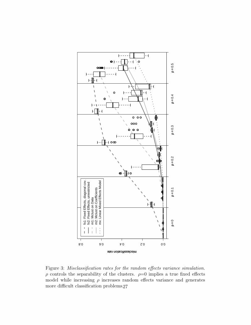
Misclassification rates are calculated by assigning each gene to the clusterwith maximum posterior probability, and are summarized in Figure 3. It issufficient to consider only small ρ since we want to see differences on the partof the curve corresponding to practical error rates. On observing the plot,we can assume that, for ρ > 0.5, clustering is too difficult and the results arenot reliable enough to draw definite conclusions.

15

We note that while Mclust on coefficients and the general covariance fixedeffects model perform similarly to each other, they outperform their respec-tive counterparts. Since they both correctly parameterize the covariance ma-trix (it is not restricted to be diagonal, or on the data scale) and since Mcluston data significantly outperforms the diagonal fixed effects model, it appearsthat ignoring the covariance structure yields a more severe penalty thanmis-parameterizing the mean. Since the differences between the two Mclustmodels and between Mclust on coefficients and the linear mixed model are in-creasingly careful parameterizations of the covariance structure, a principledconsideration of the sources of variation is favorable.

4.3 Effect of Singleton Genes

An exploratory data analysis (Eng et al., 2007) uncovered a multiplicity ofweak signals, a setting where we determined empirically that Mclust failsto find subtle patterns in favor of more general ones. Here, weak meansthat a true cluster may be represented by few genes or even that a singlegene may be its own cluster. Since all the methods produce a measure ofclustering uncertainty, we can, adjust their classification rules by thresholdingthe maximum posterior probabilities of cluster membership. In the previoussimulation each gene is assigned to a cluster. Now, we consider rules suchthat if a gene falls below the threshold level, it is labeled a “singleton,” isassigned to no cluster and is effectively noise in the clustering.

We proceed as in the first simulation setting G = 1000 genes and choosingK = 20 clusters of 50 genes each. We pick an additional 1000 genes represent-ing singleton, i.e., un-clusterable noise genes which, while they show signal,ought not to cluster with one of the 20 test clusters. Let ϕ = 50M

1000= 1− 50K′

1000

be the proportion of the G = 1000 genes that we set to be singleton noise,for K ′ = 20 −M true clusters. So, in every simulation data set there are1000 genes of which 50K ′ are clusterable and the rest are singleton noise.

Here, ϕ represents the strength of the cluster analysis (versus per-geneanalysis) assumption. At ϕ = 0 we ought to favor per-gene analyses, whileat ϕ = 1 we argue that clustering the genes increases the sample size avail-able for better parameter estimation and hypothesis testing in downstreamanalyses. These simulations ought to give us an idea of what an appropriateamount of “clusterability” looks like and how each method performs underthis setting. Note that by design, each cluster stays the same size so thatfor increasing ϕ, the signal present from a single cluster does not degenerate

16

(only the number of clusters decreases).For fixed ϕ, we fit the candidate models for the corresponding K ′ and

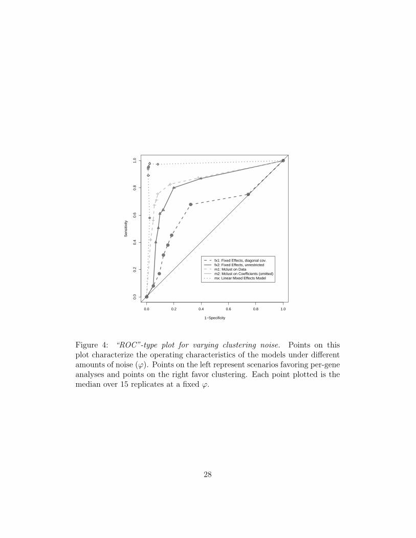
computing the probability of cluster membership for each gene. We pickgenes with low maximum posterior probabilities (less than 0.5) to be single-tons. Thus as a function of ϕ, we classify each gene as either Clusterableor Noise. Since we know their true classification we may compute operatingcharacteristics and produce a sort of Receiver Operating Curve (ROC) plot(Figure 4), characterizing different true data scenarios using ROC intuition.We define sensitivity and specificity as follows,

Sensitivity = P (Call Noise|True Noise), (18)

1− Specificity = P (Call Noise|True Clusterable), (19)

defining 1− Specificity = 0 when K ′ = 0 and Sensitivity = 1 when K ′ = 20.For each ϕ we conduct 15 simulations and plot the median of the estimatedoperating characteristics. Points on the left of the plot (1− Specificity = 0)favor per-gene analyses (many heterogenous signals) while points on the right(1− Specificity = 1) favor clustering analyses.

[Figure 4 about here.]

As we move towards ϕ = 1, where all genes are clusterable, sensitivity im-proves. We can see the added benefit of allowing general covariance structureby comparing the two fixed effects models. The standard fixed effects modelcannot isolate singleton noise when the proportion is very small while thefixed effects with unrestricted covariance performs much better. Mclust ondata holds an advantage over both of these possibly because it has a greaternumber of mean parameters and covariance parameters to work with. Weexpect the mixed effects model to perform adequately since it represents thegenerating model, but good performance at small ϕ is not guaranteed. It isreassuring to see that even for a small proportion of clusterable genes, themodel is still able to pick out singleton signals.

5 Discussion

We have presented a model for analyzing gene expression experiments whosedesigns incorporate species information as another factor in the time course

17

microarray experiment. Taking full advantage of high throughput technol-ogy, biologists can characterize complex gene processes and their conservationacross species with these designs and this model. While model based cluster-ing techniques with unspecified mean structures work adequately in simplegene expression experiments, they fail to capture important differences basedon experimental conditions, when further covariate information is available.We show that ad hoc adaptations of these models using transformed datawork well and that the class of regression based clustering models incorpo-rates the transformation and clustering in a single framework. Further, wedemonstrated that it is necessary to consider models which carefully param-eterize variance components as well. Accounting for the dependence betweentime points and the dependence between species leads to stable estimates,strong noise detection and thereby overall improvement in clustering.

Technically, we find further need for the development of a criterion forchoosing the number of clusters in a mixture model. Recalling that there isno guarantee for BIC’s performance in mixture models (Fraley and Raftery,1998), we find this mixture of regressions a particular case for further study.

Acknowledgements

We thank Audrey Gasch (UW-Madison, Department of Genetics) and DanKvitek (former Gasch Lab member) for sharing their yeast data with usbefore publication and Dan Kvitek for building the sequence tree. Thiswork was supported by NSF grant DMS-0604572 (GW), ONR N0014-06-0095 (GW), a PhRMA Foundation Research Starter Grant (SK) and NIHgrants HG03747-01 (SK) and EY09946 (GW).

Supplementary Materials

The high resolution heat maps (image plots) and the silhouette plots refer-enced in Section 3 are available at the authors’ website http://www.stat.wisc.edu/~keles/CLMM/CLMM-Supplement.zip.

18

References

Bar-Joseph, Z., Gerber, G. K., Gifford, D. K., Jaakkola, T. S., and Simon,I. (2002). A new approach to analyzing gene expression time series data.In Proceedings of RECOMB April 18-21, 2002. Washington, DC USA.

Britten, R. J. and Davidson, E. H. (1969). Gene regulation for higher cells:a theory. Science 165, 349–357.

Chu, S., DeRisi, J., Eisen, M., Mulholland, J., and Bostein, D. (1998). Thetranscriptional program of sporulation in budding yeast. Science 282,699–705.

Consortium, T. R. (2005). Standardizing global gene expression analysisbetween laboratories and across platforms. Nature Methods 2, 351–6.

Corrada Bravo, H., Eng, K. H., Keles, S., Wahba, G., and Wright, S. (2008).Estimating tree-structured covariance matrices with mixed integer pro-gramming. Department of Statistics, University of Wisconsin-MadisonTechnical Report No.1142.

Dempster, A., Laird, N. M., and Rubin, D. B. (1977). Maximum likelihoodfrom incomplete data via the em algorithm. Journal of the Royal StatisticalSociety 39, 1–22.

Eng, K. H., Corrada Bravo, H., Wahba, G., and Keles, S. (2008). A phylo-genetic mixture model for gene expression data. (Submitted.).

Eng, K. H., Kvitek, D., Keles, S., and Gasch, A. (2008). An evolutionaryanalysis of heat shock stress response in saccharomyces cerevisiae. (InPreparation).

Eng, K. H., Kvitek, D., Wahba, G., Gasch, A., and Keles,S. (2007). Exploratory statistical analysis of multi-speciestime course gene expression data. In Proceedings ofthe 56th Session of the International Statistical Institute.http://www.stat.wisc.edu/~keles/Papers/ISI2007_final.pdf.

Fay, J. C., McCullough, H. L., Sniegowski, P. D., and Eisen, M. B. (2004).Population genetic variation in gene expression is associated with pheno-typic variation in saccharomyces cerevisiae. Genome Biology 5, R26.

19

Felsenstein, J. (1973). Maximum-likelihood estimation of evolutionary treesfrom continuous characters. American Journal of Human Genetics 25,471–492.

Fraley, C. and Raftery, A. E. (1998). How many clusters? which clusteringmethod? answers via model-based cluster analysis. The Computer Journal41,.

Fraley, C. and Raftery, A. E. (2002). Model-based clustering, discriminantanalysis, and density estimation. Journal of the American Statistical As-sociation 97, 611–631.

Freckleton, R. P., Harvey, P. H., and Pagel, M. (2002). Phylogenetic anal-ysis and comparative data: a test and review of evidence. The AmericanNaturalist 160, 712–726.

Gasch, A. P., Spellman, P. T., Kao, C. M., Carmel-Harel, O., Eisen, M. B.,Storz, G., Botstein, D., and Brown, P. O. (2000). Genomic expressionprograms in the response of yeast cells to environmental changes. MolecularBiology of the Cell 11, 4241–4257.

Gilad, Y., Oshlack, A., Smyth, G. K., Speed, T. P., and White, K. P. (2006).Expression profiling in primates reveals a rapid evolution of human tran-scription factors. Nature 440, 242–5.

Gu, X. (2004). Statistical framework for phylogenomic analysis of gene familyexpression profiles. Genetics 167, 531–542.

Guo, H., Weiss, R. E., Gu, X., and Suchard, M. (2006). Time squared: re-peated measures on phylogenies. Molecular Biology and Evolution Advanceaccess: November 1, 2006.

Kerr, M. K. and Churchill, G. A. (2001). Statistical design and analysis ofgene expression microarray data. Genetical Research 77, 123–128.

Khaitovich, P., Weiss, G., Lachmann, M., Hellmann, I., Enard, W., Muet-zel, B., Wirkner, U., W., A., and Paabo., S. (2004). A neutral model oftranscriptome evolution. PLoS Biology 2, 682–689.

Kimura, M. (1991). Recent development of the neutral theory viewed fromthe wrightian tradition of theoretical population genetics. Proceedings ofthe National Academy of Sciences 88, 5969–5973.

20

King, M. C. and Wilson, A. C. (1975). Evolution at two levels in humansand chimpanzees. Science 188, 107–116.

Luan, Y. and Li, H. (2003). Clustering of time-course gene expression datausing a mixed-effects model with b-splines. Bioinformatics 19, 474–482.

Ma, P. and Zhong, W. (2008). Penalized Clustering of Large Scale Func-tional Data with Multiple Covariates. Journal of the American StatisticalAssociation 103, 625–636.

McCullagh, P. (2006). Structured covariance matrices in multivariate re-gression models. Technical report, Department of Statistics, University ofChicago.

McCulloch, C. E. and Searle, S. R. (2001). Generalized, Linear and MixedModels. Wiley.

McLachlan, G. J. and Krishnan, T. (1996). The EM algorithm and its ex-tensions. Wiley.

Ng, S. K., McLachlan, G. J., Wang, K., Ben-Tovim Jones, L., and Ng, S. W.(2003). A mixture model with random-effects components for clusteringcorrelated gene-expression profiles. Bioinformatics 22, 1745–1752.

Nuzhdin, S. V., Wayne, M. L., Harmon, K., and McIntyre, L. M. (2004).Common pattern of evolution of gene expression level and protein sequencein drosophila. Molecular Biology and Evolution 21, 1308–1317.

Qin, L. X. and Self, S. G. (2006). The clustering of regression models methodwith applications in gene expression data. Biometrics 62, 526–533.

Rifkin, S. A., Kim, J., and White, K. P. (2003). Evolution of gene expressionin the drosophila melanogaster subgroup. Nature Genetics 33, 138–144.

Schwarz, G. (1978). Estimating the dimension of a model. Annals of Statistics6, 461–464.

Smyth, G. K., Yang, Y. H., and Speed, T. P. (2003). Statistical issues inmicroarray data analysis. Methods in Molecular Biology 224, 111–136.

21

Spellman, P. T., Sherlock, G., Zhang, M. Q., Iyer, V. R., Anders, K., Eisen,M. B., Brown, P. O., Botstein, D., and Futcher, B. (1998). Comprehen-sive identification of cell cycle-regulated genes of the yeast saccharomycescerevisiae by microarray hybridization. Molecular Biology of the Cell 9,3273–3297.

Storey, J. D., Xiao, W., Leek, J. T., Tompkins, R. G., and Davis, R. W.(2005). Significance analysis of time course microarray experiments. Pro-ceedings of the National Academy of Sciences 102, 12837–12842.

Tai, Y. C. and Speed, T. P. (2006). A multivariate empricial bayes statisticfor replicated microarray time course data. Annals of Statistics 34, 2387–2412.

Tirosh, I., Weinberger, A., Carmi, M., and Barkai, N. (2006). A geneticsignature of interspecies variations in gene expression. Nature Genetics38, 830–834.

van der Laan, M. J. and Bryan, J. (2001). Gene expression analysis with theparametric bootstrap. Biostatistics 2, 445–461.

van der Laan, M. J., Dudoit, S., and Keles, S. (2004). Astymptotic optimalityof likelihood-based cross-vaidation. Statistical Applications in Genetics andMolecular Biology 3,.

Whitehead, A. and Crawford, D. L. (2006). Neutral and adaptive variationin gene expression. Proceedings of the National Academy of Sciences 103,5425–5430.

Wray, G. A., Hahn, M. W., Abouheif, E., Balhoff, J. P., Pizer, M., Rock-man, M. V., and Romano, L. A. (2003). The evolution of transcriptionalregulation in eukaryotes. Molecular Biology and Evolution 20, 1377–419.

Yuan, M. and Kendziorski, C. (2006). A unified approach for simultaneousgene clustering and differential expression identification. Biometrics 62,1089–1098.

22

A Appendix

A.1 EM Model Summary

Given that we only observe Yg ∈ Rn×1,

Yg |{Ug = k, agk, bgk} ∼ N(µgk, σ

2kI),

µgk = Xβk +Wagk +Mbgk,

the entire marginal model for Yg is a mixture of normal probability densities:

f(Yg) =K∑k=1

πkf(Yg|Ug = k),

assuming that πk = Pr(Ug = k). The observed data likelihood is therefore,

L(θ, π;Y ) =G∏g=1

K∑k=1

πkL(θk;Yg|Ug = k),

which we maximize with an EM algorithm. Let Z = {U, a, b} denote theunobserved random variables and ugk = 1{Ug = k} be the indicator that Ug =k. If we had observed Z with parameters η, the complete data likelihood,

L(θ, π;Y ) =∏gk

[L(θk;Yg|Ug = k)L(πk;ugk)]ugk ,

factors so that the log likelihood may be written up to additive constants as

l(θ, π, η;Y, Z) =∑gk

ugkl1(πk;Ug = k)

+∑gk

ugkl2(Ak; ag | Ug = k)

+∑gk

ugkl3(Bk; bg | Ug = k)

+∑gk

ugkl4(βk, σ2k;Yg | Ug = k, ag, bg).

While it is standard to assume that Yg is balanced, i.e., that n = STN , itappears to be unnecessary. Barring balance, one ought to choose a designwhere each time point is measured in each species at least once.

23

1. The E-step requires the following components:

V(t)gk = WA

(t)k W

′ +MB(t)k M

′ + σ2(t)k I

ugk =πkP (Yg | Ug = k)∑k′ πk′P (Yg | Ug = k′)

,

agk = A(t)k W

′V−1(t)gk (Yg −Xβ(t)

k ),

bgk = B(t)k M

′V−1(t)gk (Yg −Xβ(t)

k ),

εgk = Yg −Xβ(t)k −Wagk −Mbgk,

aagk = agka′gk + A

(t)gk − A

(t)gkW

′V−1(t)gk WA

(t)gk ,

bbgk = bgkb′gk +B

(t)gk −B

(t)gkM

′V−1(t)gk MB

(t)gk ,

eegk = ε′gk ˆεgk + tr(

(σ2(t)k I)− (σ

2(t)k )V

−1(t)gk (σ

2(t)k )

).

2. The M-step updates the parameter estimates:

π(t+1)k =

1

G

∑g

ugk,

A(t+1)k =

∑g ugkaagk∑g ugk

,

B(t+1)k =

∑g ugkbbgk∑g ugk

,

σ2(t+1)k =

∑g ugk(eegk)

n∑

g ugk,

β(t+1)k =

(∑g

ugkX′X

)−1(∑g

ugkX′(Yg −Wagk −Mbgk)

).

24

Cluster 78 n= 47 Fitted Values (Logratio)

−1012

S. c

ere

S. c

ere

S. c

ere

S. c

ere

S. c

ere

S. c

ere

S. k

udr

S. m

ika

S. p

ara

S. p

ara

BY

4743

S28

8CK

9M

22R

M11

aY

PS

163

IFO

1802

IFO

1815

CB

S43

2Y

−172

17Species

Strain

Figure 1: Trace Plot of an example cluster from mixed effects clusteringmodel fit. Gene specific fitted values are plotted in grey and the averagefitted value is plotted in black. Each trace spans 5 minutes to 120 minutespost heat shock. 25

Seq

uenc

e−ba

sed

tree

(Spe

cies

Tre

e)

(B)

S.m

ika

IFO

1815

(B)

S.k

udr

IFO

1802

(B)

S.p

ara

CB

S43

2 (B

) S

.par

a Y

−17

217

(B)

S.c

ere

BY

4743

(G

) S

.cer

e S

288C

(G

) S

.cer

e K

9

(G

) S

.cer

e M

22

(G

) S

.cer

e R

M11

a

(G)

S.c

ere

YP

S16

3

0.01

Exp

ress

ion−

base

d tr

ee(G

ene

Clu

ster

Tre

e)

(B)

S.m

ika

IFO

1815

(B)

S.k

udr

IFO

1802

(B)

S.p

ara

CB

S43

2 (B

) S

.par

a Y

−17

217

(B)

S.c

ere

BY

4743

(G

) S

.cer

e S

288C

(G

) S

.cer

e Y

PS

163

(G)

S.c

ere

RM

11a

(G

) S

.cer

e K

9

(G

) S

.cer

e M

22

0.01

Figure 2: Phylogenetic Tree Estimates. The tree derived from DNA sequencedata shows a similar ordering for the similarity of the species as the tree de-rived from gene expression. While a confounding laboratory effect is presentfor the expression tree, we find it to be consistent with the sequence tree.(G)asch and (B)arkai pre-scripts indicate which laboratory prepared eachstrain.

26

●●● ●●

●●●●●●

● ● ●

● ●●

● ●● ●● ●

●

● ● ●

● ● ●● ● ●● ● ●

● ● ●

● ●●

●●●

●

●●● ● ●● ●●● ●●● ●

● ● ●●

misclassification rate

0.00.20.40.60.8

ρρ==

0ρρ

==0.

1ρρ

==0.

2ρρ

==0.

3ρρ

==0.

4ρρ

==0.

5

●●● ●●

●●●●●●

● ● ●

● ●●

● ●● ●● ●

●

● ● ●

● ● ●● ● ●● ● ●

● ● ●

● ●●

●●●

●

●●● ● ●● ●●● ●●● ●

● ● ●●

misclassification rate

fx1:

Fix

ed E

ffect

s, d

iago

nal c

ov.

fx2:

Fix

ed E

ffect

s, u

nres

tric

ted

m1:

Mcl

ust o

n D

ata

m2:

Mcl

ust o

n C

oeffi

cien

tsm

x: L

inea

r M

ixed

Effe

cts

Mod

el

Figure 3: Misclassification rates for the random effects variance simulation.ρ controls the separability of the clusters. ρ=0 implies a true fixed effectsmodel while increasing ρ increases random effects variance and generatesmore difficult classification problems.27

0.0 0.2 0.4 0.6 0.8 1.0

0.0

0.2

0.4

0.6

0.8

1.0

1−Specificity

Sen

sitiv

ity

●

●

●

●

●

●

●

●

●●

fx1: Fixed Effects, diagonal cov.fx2: Fixed Effects, unrestrictedm1: Mclust on Datam2: Mclust on Coefficients (omitted)mx: Linear Mixed Effects Model

Figure 4: “ROC”-type plot for varying clustering noise. Points on thisplot characterize the operating characteristics of the models under differentamounts of noise (ϕ). Points on the left represent scenarios favoring per-geneanalyses and points on the right favor clustering. Each point plotted is themedian over 15 replicates at a fixed ϕ.

28

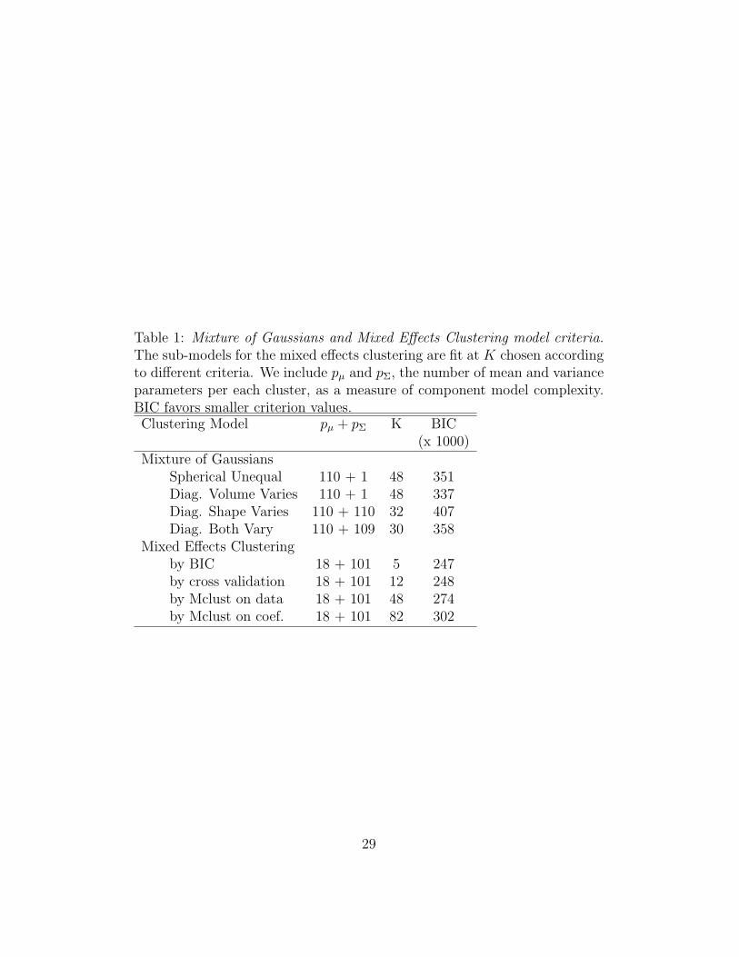
Table 1: Mixture of Gaussians and Mixed Effects Clustering model criteria.The sub-models for the mixed effects clustering are fit at K chosen accordingto different criteria. We include pµ and pΣ, the number of mean and varianceparameters per each cluster, as a measure of component model complexity.BIC favors smaller criterion values.Clustering Model pµ + pΣ K BIC

(x 1000)Mixture of Gaussians

Spherical Unequal 110 + 1 48 351Diag. Volume Varies 110 + 1 48 337Diag. Shape Varies 110 + 110 32 407Diag. Both Vary 110 + 109 30 358

Mixed Effects Clusteringby BIC 18 + 101 5 247by cross validation 18 + 101 12 248by Mclust on data 18 + 101 48 274by Mclust on coef. 18 + 101 82 302

29