A linear model for the structure of turbulence beneath surface water waves Article

Accepted Version

Teixeira, M. A.C. (2011) A linear model for the structure of turbulence beneath surface water waves. Ocean modelling, 36 (1­2). pp. 149­162. ISSN 1463­5003 doi: https://doi.org/10.1016/j.ocemod.2010.10.007 Available at http://centaur.reading.ac.uk/29239/

It is advisable to refer to the publisher’s version if you intend to cite from the work. See Guidance on citing .Published version at: http://dx.doi.org/10.1016/j.ocemod.2010.10.007

To link to this article DOI: http://dx.doi.org/10.1016/j.ocemod.2010.10.007

Publisher: Elsevier Inc.

All outputs in CentAUR are protected by Intellectual Property Rights law, including copyright law. Copyright and IPR is retained by the creators or other copyright holders. Terms and conditions for use of this material are defined in the End User Agreement .

www.reading.ac.uk/centaur

CentAUR

Central Archive at the University of Reading

Reading’s research outputs online

A linear model for the structure of turbulence

beneath surface water waves

M. A. C. Teixeira∗

CGUL, IDL, University of Lisbon, Lisbon, Portugal

Abstract

The structure of turbulence in the ocean surface layer is investigated using

a simplified semi-analytical model based on rapid-distortion theory. In this

model, which is linear with respect to the turbulence, the flow comprises a

mean Eulerian shear current, the Stokes drift of an irrotational surface wave,

which accounts for the irreversible effect of the waves on the turbulence,

and the turbulence itself, whose time evolution is calculated. By analysing

the equations of motion used in the model, which are linearised versions of

the Craik-Leibovich equations containing a ‘vortex force’, it is found that

a flow including mean shear and a Stokes drift is formally equivalent to a

flow including mean shear and rotation. In particular, Craik and Leibovich’s

condition for the linear instability of the first kind of flow is equivalent to

Bradshaw’s condition for the linear instability of the second. However, the

present study goes beyond linear stability analyses by considering flow distur-

bances of finite amplitude, which allows calculating turbulence statistics and

addressing cases where the linear stability is neutral. Results from the model

∗Corresponding author: M. A. C. Teixeira, Centro de Geofısica da Universidade deLisboa, Edifıcio C8, Campo Grande, 1749-016 Lisbon, Portugal

Email addresses: mateixeira@fc.ul.pt (M. A. C. Teixeira)

Preprint submitted to Ocean Modelling October 15, 2010

show that the turbulence displays a structure with a continuous variation of

the anisotropy and elongation, ranging from streaky structures, for distor-

tion by shear only, to streamwise vortices resembling Langmuir circulations,

for distortion by Stokes drift only. The TKE grows faster for distortion by

a shear and a Stokes drift gradient with the same sign (a situation relevant

to wind waves), but the turbulence is more isotropic in that case (which is

linearly unstable to Langmuir circulations).

Key words: Langmuir circulation, Turbulent boundary layer, Wave drift

velocity, Shear flow, Rapid-distortion theory

1. Introduction

Turbulent shear flows beneath surface waves in the upper ocean are char-

acterised by a number of intriguing features that need to be better under-

stood. For example, the turbulence is often dominated by elongated vortices

with their axes of rotation aligned in the streamwise direction, i.e. the di-

rection of the wind stress and of wave propagation (Faller and Auer, 1988).

These vortices have been identified with Langmuir circulations (Leibovich,

1983), prompting McWilliams et al. (1997) to coin the term ‘Langmuir tur-

bulence’. The structure of Langmuir turbulence contrasts with the structure

of turbulence typical of boundary layers near flat boundaries, where the flow

is dominated by ‘streaky structures’ (Kline et al., 1967), which are elongated

fluctuations of the streamwise velocity component. Thais and Magnaudet’s

(1996) laboratory experiments of turbulence beneath surface waves sheared

by the wind have shown that, even when there are no Langmuir circulations

as usually defined, the turbulence is more isotropic than expected near a flat

2

boundary and the TKE level is higher.

Langmuir circulations have been explained by Craik and Leibovich (1976),

Craik (1977) and Leibovich (1980) as being due to an instability associated

with the interaction between the shear current induced by the wind and the

Stokes drift of surface waves, but in these studies turbulence was ignored,

except as a diffusive process. In a series of papers, Craik (1982), Phillips and

Wu (1994) and Phillips et al. (1996) investigated theoretically the instabil-

ity of flows with strong shear near wavy boundaries to streamwise vortices.

These studies have shown that the basic factors affecting the stability of

the flow to perturbations are the shape of the mean velocity profile and the

shape of the pseudo-momentum profile (which replaces the Stokes drift as a

key parameter for strongly sheared flows) (Andrews and McIntyre, 1978).

Craik and Leibovich’s and Phillips’ studies treat the generation of stream-

wise vortices essentially from a linear stability analysis perspective. A theo-

retical understanding of Langmuir circulations at stages subsequent to insta-

bility, when fully developed turbulence exists, requires the use of statistical

methods. A first attempt at tackling this problem was made by Teixeira and

Belcher (2002). Using an idealised linear model based on rapid distortion

theory (RDT), they found that initially isotropic turbulence distorted by a

surface wave becomes anisotropic in a way consistent with the existence of

intense and elongated streamwise vortices. This process is associated with

the transfer of energy from the waves to the turbulence, which leads to a

decay of the waves. This wave decay was evaluated using real ocean data by

Ardhuin and Jenkins (2006) and Kantha et al. (2009). As in Craik and Lei-

bovich’s theory, the Stokes drift of the wave is essential in the process studied

3

by Teixeira and Belcher (2002), but acts by distorting the vorticity of the

turbulence, so the existence of mean shear is not required. Turbulence acts

in this case as the source of the streamwise vortices instead of a dissipative

process that limits their growth. According to Teixeira and Belcher (2010),

the neglect of shear may be acceptable at late stages in the development of

Langmuir circulations, when extensive vertical mixing has taken place, but

that is not always the case.

The turbulent shear flow beneath surface waves comprises three basic

components: turbulence, a mean Eulerian shear current (induced by the

wind stress, by wave breaking, or by viscous boundary layer effects) and

the orbital motion of the waves. These three flow components interact in

a complex way. The turbulence generally extracts energy from the shear

and the wave motion, and the anisotropy of the turbulence is shaped by

the distortions caused by the other components of the flow. The distortion

by shear, which gives rise to the typical turbulence anisotropy in flat-wall

boundary layers, has been studied extensively using RDT (Townsend, 1970;

Gartshore et al., 1983; Lee et al., 1990), but the distortion by the wave

motion is more subtle and less well understood. This study aims to extend

the RDT model of Teixeira and Belcher (2002) to include the distorting effect

of shear, thereby approximating better the dynamics of real boundary layers.

As in Teixeira and Belcher (2002), the Stokes drift of surface waves will be

treated as equivalent to a purely irrotational straining.

As noted by Shrira (1993), when surface waves propagate in a homoge-

neous fluid with a non-uniform velocity profile, there is only one situation

where the wave motion remains irrotational: when the shear rate is con-

4

stant and the shear is aligned with the wavenumber vector. Only in that

case can the Stokes drift gradient be considered as strictly equivalent to an

irrotational straining. Generally, this is not so. The existence of either cur-

vature in the mean velocity profile or an angle between the mean shear and

the wavenumber vector renders the wave motion (and the associated Stokes

drift) rotational. This makes the dynamics of the motion more complicated

and requires the introduction of a generalised Stokes drift with non-zero vor-

ticity (Phillips, 2001). This problem is especially acute in the atmosphere

(Phillips and Wu, 1994). In the ocean, the waves are observed to be approx-

imately irrotational, perhaps due to the relative weakness of shear currents,

and this is taken here as an indication that the adoption of an irrotational

Stokes drift is acceptable. Incidentally, this is also the approach used in nu-

merous large-eddy simulation (LES) studies of the oceanic boundary layer

(McWilliams et al., 1997; Li et al., 2005; Polton and Belcher, 2007; Grant and

Belcher, 2009), when they adopt equations including Craik and Leibovich’s

‘vortex force’, which assumes irrotational wave motion. This provides some

reassurance that the present approach is sound.

In this study, the simplest situation of shear–Stokes drift–turbulence in-

teraction is considered: a flow where the shear of the mean Eulerian current

and the Stokes drift are aligned and where the gradients of both transports

are approximated as (at least locally) constant (cf. Teixeira and Belcher,

2010). As seen above, this approach is self-consistent, and the Stokes drift

gradient can be viewed simply as a vertical velocity gradient which has no

vorticity associated.

This paper is organised as follows. Section 2 discusses the theoretical

5

model used in this study. In Section 3, various statistics of the turbulence

are presented for different relative magnitudes of shear and Stokes drift.

That section contains an analysis of the energy budget of the turbulence

and a physical interpretation of the results. Qualitative and quantitative

comparisons of the results with available data are also carried out. Finally,

Section 4 presents the main conclusions of this study.

2. Turbulence distorted by shear and a Stokes drift

Like all models based on RDT, the present model is linearised with re-

spect to the turbulence (Batchelor and Proudman, 1954). Formally, this

linearisation is approximately valid if the strain rate imposed on the turbu-

lence by the shear flow and the Stokes drift is considerably larger than the

inverse of the eddy turn-over time and if the time since the beginning of the

distortion is smaller than one eddy turn-over time. These conditions have

been extensively discussed elsewhere (Hunt and Carruthers, 1990; Kevlahan

and Hunt, 1997). Even when these conditions are not strictly satisfied, RDT

is useful because it gives the evolution of the turbulence due to external forc-

ings, and previous studies suggest that these forcings are essentially what

determines the equilibrium structure of the turbulence (Townsend, 1970; Lee

et al., 1990; Mann, 1994; Cambon and Scott, 1999).

Although RDT is closely related to linear stability theory, as pointed out

by Speziale et al. (1996) for rotating shear flows, it is more complete in a

number of ways. Firstly, it considers perturbations of a finite amplitude.

Secondly, it does not impose an exponential dependence on the time evolu-

tion of these perturbations (Hunt and Carruthers, 1990). The special cases

6

of turbulence distortion by shear only, treated by Townsend (1976), and by

Stokes drift only, treated by Teixeira and Belcher (2002, 2010), are quite

relevant physically, but they are linearly neutral because the perturbation

energy grows at an algebraic rate. Thirdly, unlike linear stability analysis,

RDT considers a spectrum of perturbations. This is much more appropriate

for describing the structure of real flows, where the turbulence contains a

variety of scales, and Reynolds stresses and dissipation rates are the mea-

sured or diagnosed quantities (see for example Thais and Magnaudet, 1996;

McWilliams et al., 1997, Teixeira and Belcher, 2000).

The momentum equation adopted in this study can be expressed as

∂u

∂t+ U · ∇u + u · ∇U = −1

ρ∇p′ + US × ω, (1)

where u is the turbulent velocity, ω = ∇× u is the turbulent vorticity, U is

the mean Eulerian velocity, US is the Stokes drift velocity, ρ is the density

(assumed to be constant) and

p′ = p + ρUS · u (2)

is a turbulent pressure that includes a correction due to the Stokes drift, as

in equation (2.1) of McWilliams et al. (1997). Note that (1) is a linearised

and inviscid version of the Craik-Leibovich momentum equation (Leibovich,

1983). Gravity does not appear in this equation because it is assumed to

be balanced exactly by the mean pressure in the bulk of the fluid through

hydrostatic equilibrium. The last term on the right is the ‘vortex force’ term

introduced to parameterise the Lagrangian-mean effect of the Stokes drift.

The corrected pressure p′ is also a linearised version of the corresponding

quantity (called π) used by McWilliams et al. (1997). The Craik-Leibovich

7

momentum equation, from which (1) results, can be derived through suitable

averaging of the fundamental equations including the wave motion (Craik

and Leibovich, 1976), or directly from the basic generalised-Lagrangian-mean

equations (Andrews and McIntyre, 1978) assuming that the flow perturba-

tions are irrotational (see also Ardhuin et al., 2008). This approach is not

incompatible with the simulation of turbulent flows, since in the momentum

equation the turbulent velocity may be grouped in with the rotational mean

flow. This is in fact consistent with the RDT assumptions, since the turbu-

lent flow is assumed to be much slower than the wave orbital motions and

hence can be considered itself a mean flow from the viewpoint of averaging

with respect to the wave oscillations.

The mass conservation equation for the turbulence, valid for incompress-

ible flow,

∇ · u = 0, (3)

completes the set from which u and p′ can be determined. An alternative

equation set can be formed with (1) and the equation obtained by taking the

divergence of (1) and using (3):

∇2p′ = ρ∇ · [(U + US)× ω] +∇ · [u× (∇×U)]−∇2(U · u)

, (4)

which gives the corrected pressure.

For simplicity, in the present model both U and US are assumed to de-

pend only on z (the vertical coordinate) and US is assumed to be aligned

in the x (hereafter called the streamwise) direction. U may not be aligned

in the x direction, but only its x component U is assumed to vary with z.

The component of the Eulerian flow along y (hereafter called the spanwise

8

direction), V , is dynamically irrelevant, since it is assumed to be constant,

and can be eliminated through a simple Galilean transformation. The possi-

bility V 6= 0 is contemplated because typically the Eulerian current existing

at the water surface is misaligned with the wind stress due to Ekman layer

effects (Ardhuin et al., 2009). However, the vertical gradient of this current

(which is proportional to the wind stress) is approximately aligned with the

the wavenumber vector of the dominant surface waves, and therefore with

their Stokes drift, at least near the surface. The effect of the Earth’s rotation

on the turbulent motion is approximately negligible, as shown by Grant and

Belcher (2009). All of these aspects are consistent with the assumptions of

the model.

A Lagrangian mean velocity may be defined as

UL(z) = U(z) + US(z). (5)

This is the velocity at which fluid parcels are advected on average. It is also

possible to define a parameter α such that

dU

dz= α

dUL

dz,

dUS

dz= (1− α)

dUL

dz.

(6)

This parameter controls the relative importance of the distortion by shear

and by Stokes drift. When α = 0, the distorting mean flow has no vorticity,

i.e. it is an irrotational Stokes drift, whereas when α = 1, the distorting

mean flow is a pure shear flow. For values of α between 0 and 1, the vertical

gradients the Eulerian shear flow and of the Stokes drift have the same sign.

Outside this interval, the gradients of the Stokes drift and of the shear flow

are of opposite signs (see Fig. 1). The case 0 < α < 1 is applicable, for

9

example, to wind waves, whereas the cases α < 0 or α > 1 may correspond

to waves propagating against the wind. The case α = 0 could apply to

situations of swell, or of waves propagating over a well-mixed surface layer.

As is usual in RDT, the mean transport gradients (associated with the

shear flow and with the Stokes drift) are assumed to be slowly varying, and

the turbulence is assumed to be locally homogeneous. Then, at each point

the turbulent velocity and pressure can be expressed as Fourier integrals,

u(x, t) =

∫∫∫u(k, t)eik·xdk1dk2dk3,

p′(x, t) =

∫∫∫p′(k, t)eik·xdk1dk2dk3,

(7)

where u and p′ are the corresponding Fourier transforms and k(t) = (k1, k2, k3(t))

is the wavenumber vector (cf. Teixeira and Belcher, 2010). The fact that k

depends on time is a consequence of the distortion of the turbulence by the

mean transport gradients.

Introducing the definitions of u and p′ given by (7) into (1) and (4),

equations may be derived for the Fourier transforms of the turbulent velocity

and pressure. The Fourier transform of (4) provides a definition for p′, which

may be used in the Fourier transform of (1) to eliminate the pressure. This

is an important advantage of the spectral formulation used in RDT.

Since the turbulence is random, the primary interest here is in the evo-

lution of the turbulent velocity spectra. Equations for these can be derived

by multiplying the equations giving the evolution of the Fourier transforms

ui by the complex conjugate of each Fourier transform, ensemble averaging

and noting that

u∗i (k, t)uj(k′, t) = Φij(k, t)δ(k− k′), i, j = 1, 2, 3, (8)

10

by definition, where Φij is the three-dimensional wavenumber spectrum of

the turbulent velocity, δ is the Dirac delta, the asterisk denotes complex

conjugate and the overbar denotes ensemble averaging.

From (8) it can be seen that Φij, when real, is symmetric. The equations

for the six independent components of this tensor are:

∂Φ11

∂t= 2(1− α)

k1k3

k2

dUL

dzΦ11 − 2

[α− (1 + α)

k21

k2

]dUL

dzΦ13,

∂Φ33

∂t= 2(1 + α)

k1k3

k2

dUL

dzΦ33 − 2(1− α)

k212

k2

dUL

dzΦ13,

∂Φ22

∂t= 2

k2

k2

dUL

dz[(1 + α)k1Φ23 + (1− α)k3Φ12] ,

∂Φ13

∂t= 2

k1k3

k2

dUL

dzΦ13 −

[α− (1 + α)

k21

k2

]dUL

dzΦ33

−(1− α)k2

12

k2

dUL

dzΦ11,

∂Φ12

∂t= (1− α)

k1k3

k2

dUL

dzΦ12 −

[α− (1 + α)

k21

k2

]dUL

dzΦ23

+k2

k2

dUL

dz[(1 + α)k1Φ13 + (1− α)k3φ11] ,

∂Φ23

∂t= (1 + α)

k1k3

k2

dUL

dzΦ23 − (1− α)

k212

k2

dUL

dzΦ12

+k2

k2

dUL

dz[(1 + α)k1Φ33 + (1− α)k3Φ13] .

(9)

Note that these equations are expressed in terms of dUL/dz and α, showing

that the vertical gradient of the total Lagrangian mean velocity is responsible

for the distortion of the turbulence. A natural dimensionless time suggested

by the equations is

β =dUL

dzt. (10)

One additional equation must be added to (9) to give the evolution of the

wavenumber vector due to the distortion by the mean flow:

k3 = k30 − k1β, (11)

11

where k30 = k3(t = 0) is the initial value of the vertical component of the

wavenumber. Note that also this equation depends on the vertical gradient

of the Lagrangian velocity, through β. The other components (k1 and k2)

are unaffected by the transport gradients and remain unchanged.

This study aims to investigate the structure of the turbulence, and for that

purpose correlations and integral length scales of the turbulent velocity will

be calculated. At any time, the velocity variances or one-point correlations

are given by the expression

uiuj =

∫∫∫Φijdk1dk2dk3, (12)

where i, j = 1, 2, 3, while the integral length scales are given by

Lxij = π

∫∫Φij(k1 = 0)dk2dk3

uiuj

(13)

along the x direction, with analogous definitions for the y direction. The

velocity variances and correlations give information about the turbulence

energy and anisotropy. The integral length scales give information about the

distances over which the turbulence velocities lose their coherence, and can

be used to characterise the turbulence elongation.

In line with previous RDT treatments (Townsend, 1970; Mann, 1994;

Teixeira and Belcher, 2002, 2010), the turbulence is assumed to be initially

isotropic, so that

uiuj(t = 0) = q2δij, (14)

where q is the initial root-mean-square (RMS) velocity and δij is the Kro-

necker delta. If l is defined as the initial longitudinal integral length scale,

then

Lxmii (t = 0) = l if i = m, Lxm

ii (t = 0) = 0.5l if i 6= m, (15)

12

because the longitudinal length scales are twice the transverse length scales

in isotropic turbulence.

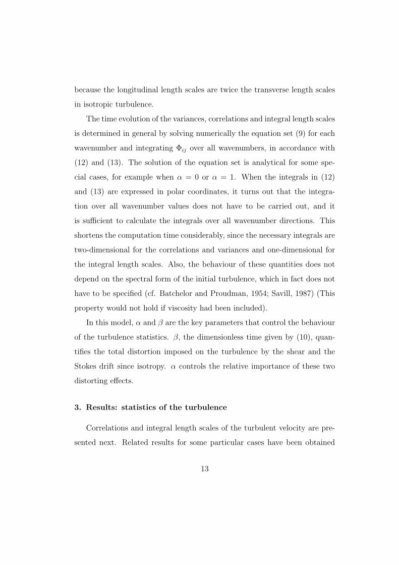
The time evolution of the variances, correlations and integral length scales

is determined in general by solving numerically the equation set (9) for each

wavenumber and integrating Φij over all wavenumbers, in accordance with

(12) and (13). The solution of the equation set is analytical for some spe-

cial cases, for example when α = 0 or α = 1. When the integrals in (12)

and (13) are expressed in polar coordinates, it turns out that the integra-

tion over all wavenumber values does not have to be carried out, and it

is sufficient to calculate the integrals over all wavenumber directions. This

shortens the computation time considerably, since the necessary integrals are

two-dimensional for the correlations and variances and one-dimensional for

the integral length scales. Also, the behaviour of these quantities does not

depend on the spectral form of the initial turbulence, which in fact does not

have to be specified (cf. Batchelor and Proudman, 1954; Savill, 1987) (This

property would not hold if viscosity had been included).

In this model, α and β are the key parameters that control the behaviour

of the turbulence statistics. β, the dimensionless time given by (10), quan-

tifies the total distortion imposed on the turbulence by the shear and the

Stokes drift since isotropy. α controls the relative importance of these two

distorting effects.

3. Results: statistics of the turbulence

Correlations and integral length scales of the turbulent velocity are pre-

sented next. Related results for some particular cases have been obtained

13

by other authors for turbulence in a rotating shear flow (Speziale and Mac-

Giolla Mhuiris, 1989; Cambon et al., 1994; Salhi and Cambon, 1997), which

as will be seen is related to the present flow, but the emphasis was mainly

on the evolution of the TKE. Here the parameter regime will be explored

more systematically and attention will also be focused on measures of the

turbulence anisotropy and turbulence structure (only briefly treated by Salhi

and Cambon, 1997). Moreover, in contrast with these previous studies, the

results will be interpreted having in mind their application to the oceanic

boundary layer.

Figs. 2 to 5 show variances, correlations and integral length scales of

the turbulent velocity as a function of the dimensionless time β, and of

parameter α. A maximum value of β of 10 was chosen, because it is unlikely

that the turbulence will undergo distortions greater than this, the anisotropy

becoming too large and being limited by nonlinear processes (cf. Townsend,

1976; Lee et al., 1990). The limits of α have been chosen as -1 and 2, so

that the distortion by a Stokes drift gradient and a shear having the same

sign (the situation considered by Craik and Leibovich) occupies the central

portion of the graphs (0 < α < 1), but the parameter regime where they have

opposite signs (−1 < α < 0 or 1 < α < 2) is also considered (see Fig. 1).

It must be stressed that the results of Sections 3.1 to 3.4 are rather general,

and do not yet correspond to a particular oceanic depth. A more specific

application will be given in Section 3.7.

3.1. Reynolds stresses

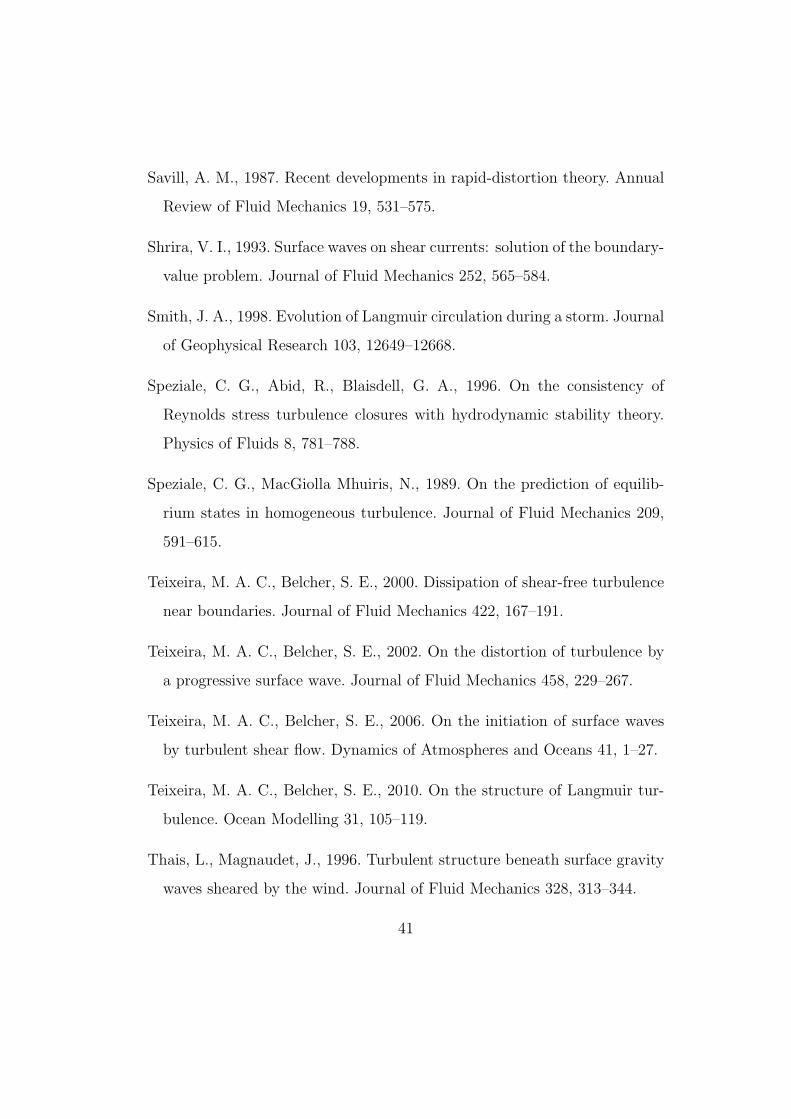
Fig. 2 shows various components of the Reynolds stress tensor normalised

by the initial RMS velocity of the turbulence, q.

14

Figs. 2a-c show the streamwise, spanwise and vertical velocity variances,

respectively u2, v2 and w2. Fig. 2d shows the TKE, which is defined as

K = (1/2)(u2 +v2 +w2), and Fig. 2e shows the shear stress, uw. All velocity

variances depart from a normalised value of one and the shear stress departs

from a value of zero, corresponding to isotropic turbulence.

When interpreting the graphs, it is useful to note that there is a con-

nection between the shear stress and the growth rate of TKE. For a flow

including Stokes drift, the mechanical production term of the TKE equation

is (McWilliams et al., 1997)

−uwdUL

dz. (16)

So the tendency of the TKE is roughly proportional to the shear stress

through straining by the Lagrangian-mean flow: a negative shear stress leads

to TKE growth while a positive shear stress leads to TKE decay.

In Fig. 2 it can be seen that when α = 0 then u2 decreases with β, while

both v2 and w2 increase at a similar rate. This leads, at large β, to a situation

where u2 ¿ (v2 ≈ w2), that is, turbulence dominated by intense vortices

with their axis of rotation aligned in the streamwise direction (Teixeira and

Belcher, 2002). The TKE increases at a moderate (algebraic) rate and uw

takes negative values.

When α = 1, then u2 and v2 both increase with β, while w2 decreases. u2

increases at a faster rate than v2, and this leads to an ordering of the variances

that becomes u2 > v2 > w2 at large β. This corresponds to turbulence

dominated by streaky structures characterised by intense streamwise velocity

fluctuations (as simulated, for example, by Lee et al., 1990). The TKE grows

faster than for α = 0 (but still algebraically), and uw is more negative, as

15

expected.

When 0 < α < 1 (shear and Stokes drift gradient with the same sign),

all the velocity variances grow very fast (approximately exponentially). For

α = 0.5 (where the maximum growth rate roughly occurs), u2 and w2 grow at

a similar rate, which is somewhat larger than the growth rate of v2. However,

the magnitude of the three variance components never differs by a large factor

and for that reason the turbulence is more isotropic than for either α = 0 or

α = 1. Obviously, in this case the TKE grows much faster and uw also takes

much larger negative values than for α = 0 or α = 1.

When α < 0 or α > 1, the Stokes drift gradient and the shear have

opposite signs. All the velocity variances decay as β increases (excepting a

short initial period of transient growth near α = 0 and α = 1), and there is

a hint in Figs. 2a,c that the velocity variances also oscillate. This behaviour

will be explained in Section 3.5. Naturally, the TKE decays in this case, and

uw is now generally small and positive, except for relatively low β and near

α = 0 or α = 1.

The rapid growth of the TKE that occurs when 0 < α < 1 and the TKE

decay when α < 0 or α > 1 (see Fig. 2d) is consistent with the instability

to Langmuir circulations, since this instability arises in neutrally stratified

inviscid flow whenever the shear and the Stokes drift gradient have the same

sign: (dU/dz)(dUS/dz) > 0 (see e.g. Leibovich, 1977). This corroborates

the known result that linear instability is included in the possible modes of

growth of disturbances in RDT (Speziale et al., 1996). However, Langmuir

circulations have usually been regarded as streamwise vortices. The present

results suggest that the only situation where pure streamwise vortices exist

16

is in the absence of shear (for α = 0). Hence the structure of Langmuir

circulations can be more complex than perceived in previous investigations.

An analysis of the turbulence anisotropy and structure will make this point

clearer.

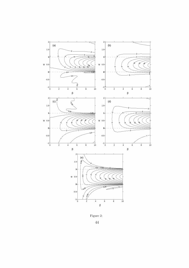
3.2. Tubulence anisotropy

Detailed information about the turbulence anisotropy can be obtained by

calculating ratios of the turbulent velocity variances and correlations. This

is done in Fig. 3.

Figs. 3a-c present ratios of the vertical to the streamwise velocity vari-

ance, w2/u2, of the vertical to the spanwise velocity variance, w2/v2, and of

the spanwise to the streamwise velocity variance, v2/u2, respectively. Given

Figs. 3a,b, the information provided by Fig. 3c is partly redundant (since

v2/u2 can be determined from w2/u2 and w2/v2). Either of these ratios can

be used as a measure to distinguish between shear turbulence (dominated

by streaky structures) and Langmuir turbulence (dominated by streamwise

vortices), since the former is characterised by w2/u2 < 1, w2/v2 < 1 and

v2/u2 < 1 and the latter by w2/u2 > 1, w2/v2 ≈ 1 and v2/u2 > 1.

It can be seen that, as β increases, w2/u2 becomes considerably larger

than 1 for α < 0.5, and smaller than 1 for α > 0.5. The highest and the

lowest values of w2/u2 are attained, respectively, for α = 0 and near α = 1

(slightly above). The region where w2/v2 ≈ 1 extends approximately from

α = 0 to a value of α between 0 and 1. This value increases from ≈ 0.2 at

low β to ≈ 0.8 at high β. Outside this range of α, w2/v2 is always lower

than 1. For high β, there is a region, near α = 0.3, where w2/v2 > 1.

This behaviour is not characteristic of pure streaky structures nor of pure

17

streamwise vortices. It can be seen that the maximum values of v2/u2 occur

at high β for α = 0. The region where v2/u2 is smaller than one ranges from

above α ≈ 0.8 at low β to above α ≈ 0.4 at higher β. v2/u2 has a minimum

for α ≈ 0.8 at high β. For α < 0 or α > 1, w2/u2, w2/v2 and v2/u2 do

not take very high or low values, remaining near one. The best criterion for

distinguishing shear turbulence from Langmuir turbulence is probably that

based on w2/u2, because it is approximately independent of β, as shown by

Fig. 3a.

These graphs clearly illustrate that the unstable perturbations that satisfy

Craik and Leibovich’s instability condition have a complex structure that

varies continuously from α = 0 to α = 1. The turbulence goes from a

state dominated by streamwise vortices (at α = 0) to a state dominated

by streaky structures (at α = 1), with an intermediate type of structure in

between. At α = 0.5 and large β, for example, u2 and w2 are similar in

magnitude, and both somewhat larger than v2, and the turbulence is more

isotropic than in either extreme case. Presumably, both streamwise vortices

and streaky structures exist in this parameter regime. Perhaps these streaky

structures existing alongside the streamwise vortices can be identified with

the surface jets that have been observed at the confluence zones of the vortices

in Langmuir circulations (Leibovich, 1983).

Fig. 3d shows the ratio of minus the shear stress to the TKE, −uw/K.

This ratio, which has been evaluated by Townsend (1976) to be ≈ 0.25

for shear flows, is slightly smaller for α = 0 than for α = 1, and when

0 < α < 1 takes considerably higher values. Additionally, when α = 0 or

α = 1 then −uw/K first increases with β, attains a maximum for some value

18

of this parameter, and finally decreases, while for 0 < α < 1 it increases

monotonically. For α < 0 or α > 1, this ratio is small and negative, due to

the fact that uw is small and positive.

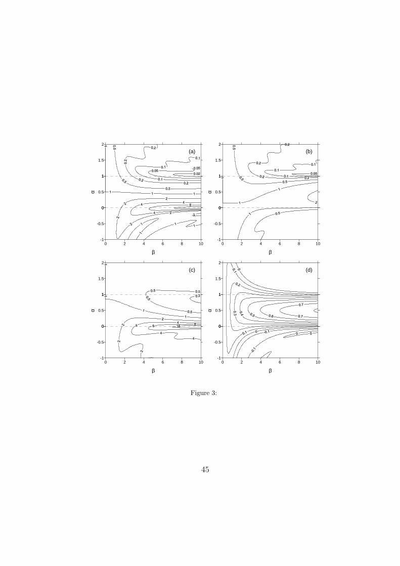
3.3. Integral length scales

Additional information about the structure of the turbulence can be ob-

tained by calculating the integral length scales of the velocity fluctuations.

These are shown in Fig. 4, normalised by the initial longitudinal integral

length scale, l. Since the turbulence is initially isotropic, all longitudinal

length scales depart from a normalised value of 1, while the transverse length

scales depart from a normalised value of 0.5.

Figs. 4a,b show, respectively, the integral length scales along x and along

y of the u velocity fluctuations, Lx11 and Ly

11. It can be seen that, if 0 < α < 1,

then Lx11 increases considerably with β while remaining with a value not very

different from one for α ≤ 0 or α ≥ 1. In contrast, Ly11 decreases as β

increases for 0 < α ≤ 1, but does not change in magnitude very much

otherwise. A somewhat similar behaviour, with some differences, can be

observed for Lx22 and Ly

22 in Figs. 4c,d and for Lx33 and Ly

33 in Figs. 4e,f. The

main differences are that Lx22 increases with β somewhat more slowly than

Lx11 and decreases instead for α = 1, and that Lx

33 does not increase with β

for α = 1. Additionally, Ly33 decreases for α = 0 but not for α = 1. These

subtle differences have important consequences for the distinct regimes of

streamwise elongation of the turbulence structures. This elongation is borne

out more clearly by plotting ratios of the integral length scales along x and

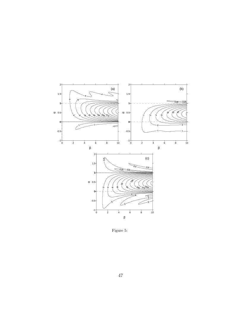
along y, as is done in Fig. 5.

19

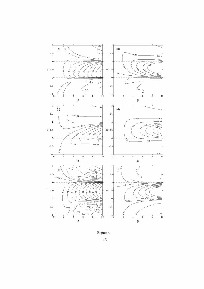
3.4. Streamwise elongation

Figs. 5a-c present graphs of the ratios Lx11/L

y11, Lx

22/Ly22 and Lx

33/Ly33.

These ratios quantify, respectively, the elongation of the u, v and w turbulent

velocity structure in an x− y cross-section.

It can be seen that Lx11/L

y11, Lx

22/Ly22 and Lx

33/Ly33 grow as β increases for

0 < α < 1, but do not grow appreciably for α < 0 or α > 1. However, there

are some subtle differences. For example, Lx11/L

y11 retains exactly its initial

value for α = 0 while it grows for α = 1. This is a manifestation of the

streamwise elongation of the streaky structures that exist in shear flow (cf.

Lee et al., 1990). No such elongation of the u velocity fluctuations exists for

distortion by an irrotational Stokes drift (α = 0). On the other hand, both

Lx22/L

y22 and Lx

33/Ly33 grow for α = 0, while not for α = 1. In particular,

Lx33/L

y33 retains exactly its initial value for α = 1. This is a manifestation of

the elongation of the streamwise vortices existing in turbulence distorted by

a Stokes drift, while no such elongation exists for distortion by shear (α = 1).

Lx11/L

y11, Lx

22/Ly22 and Lx

33/Ly33 all have a maximum growth rate near α = 0.5,

which indicates that the largest elongation of the turbulence structures in

the streamwise direction clearly occurs when both shear and a Stokes drift

gradient with the same sign are present. Such elongation exists, in this

situation, in all components of the velocity fluctuations, which is consistent

with Craik and Leibovich’s idea of seeking unstable disturbances for which

k1 = 0 (Leibovich, 1977).

3.5. Physical interpretation of the results

Following Teixeira and Belcher (2002), the evolution of the turbulent

velocity variances can be interpreted in terms of vorticity dynamics (see also

20

Teixeira and Belcher, 2010). The simplest case is turbulence distorted by

waves (α = 0), where the vertical vorticity of the turbulence is simply tilted

by the Stokes drift of the waves and amplified as streamwise vorticity. This

one-way interaction leads to the amplification of the spanwise (v) and vertical

(w) velocity fluctuations, causing the appearance of streamwise vortices.

In the case of a pure shear flow (α = 1), there are two sources of vortic-

ity: the shear and the turbulence. In a two-way interaction, the shear tilts

the turbulent vorticity in the same way as a Stokes drift, but the turbulent

velocity tilts the mean spanwise vorticity dU/dz into vertical and streamwise

vorticity (Teixeira and Belcher, 2002, Fig. 15). The streamwise vortici-

ties generated through these two processes partly cancel, so the formation

of streamwise vortices is prevented, and streaky structures appear instead,

where the streamwise velocity fluctuations (u) are dominant.

In intermediate cases, when shear and a Stokes drift gradient with the

same sign distort the turbulence, there are still two sources of vorticity, but

the shear constitutes a smaller fraction of the total strain than in the previous

case. So the cancellation of streamwise mean and turbulent vorticity does

not occur, and streamwise vortices, as well as streaky structures, should be

generated. The absence of vorticity cancellation also leads to an instability

characterised by exponential growth of the TKE (as will be shown more

explicitly next). When the shear and the Stokes drift gradient have different

signs, this interpretation based on vorticity dynamics appears not to be as

simple, but it is clear that there must occur a certain deal of cancellation of

the two strains.

The dynamics of the turbulence can be better understood if one analyses

21

the equations giving the evolution of the TKE and of the shear stress. The

TKE equation can be derived by multiplying the momentum equation (1) by

u and ensemble averaging. The result is

∂K

∂t+ UL · ∇K = −uw

dUL

dz− 1

ρ∇ · (pu). (17)

Dissipation is omitted because it is neglected in the rapid-distortion approach

used here. If it is further noted that the turbulence is assumed to be approxi-

mately homogeneous, the turbulent correlations and variances do not depend

appreciably on position, and their spatial gradients are approximately zero.

Therefore, subject to the assumptions of the present model, (17) reduces to

dK

dt= −uw

dUL

dz. (18)

Hence the production of TKE by shear and by straining by the Stokes drift

(both contained in dUL/dz) is the only reason why the TKE evolves in time.

In order to understand this evolution, it is useful to derive an equation for

the shear stress. This can be obtained by multiplying the vertical component

of (1) by u, adding it to the x component of (1) multiplied by w, ensemble

averaging and rearranging. This yields

duw

dt= −w2

dU

dz− u2

dUS

dz− 1

ρ

(w

∂p

∂x+ u

∂p

∂z

). (19)

In its present form, this equation is of little use because the time dependence

of u2 and w2 is unknown. To circumvent this problem, equations may be

derived for the evolution of these two quantities, using again the momentum

equation, (1):

du2

dt= −2uw

dU

dz− 2

ρu

∂p

∂x,

dw2

dt= −2uw

dUS

dz− 2

ρw

∂p

∂z.

(20)

22

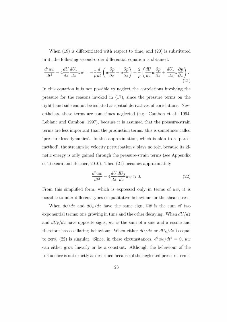
When (19) is differentiated with respect to time, and (20) is substituted

in it, the following second-order differential equation is obtained:

d2uw

dt2− 4

dU

dz

dUS

dzuw = −1

ρ

d

dt

(w

∂p

∂x+ u

∂p

∂z

)+

2

ρ

(dU

dzw

∂p

∂z+

dUS

dzu

∂p

∂x

).

(21)

In this equation it is not possible to neglect the correlations involving the

pressure for the reasons invoked in (17), since the pressure terms on the

right-hand side cannot be isolated as spatial derivatives of correlations. Nev-

ertheless, these terms are sometimes neglected (e.g. Cambon et al., 1994;

Leblanc and Cambon, 1997), because it is assumed that the pressure-strain

terms are less important than the production terms: this is sometimes called

‘pressure-less dynamics’. In this approximation, which is akin to a ‘parcel

method’, the streamwise velocity perturbation v plays no role, because its ki-

netic energy is only gained through the pressure-strain terms (see Appendix

of Teixeira and Belcher, 2010). Then (21) becomes approximately

d2uw

dt2− 4

dU

dz

dUS

dzuw ≈ 0. (22)

From this simplified form, which is expressed only in terms of uw, it is

possible to infer different types of qualitative behaviour for the shear stress.

When dU/dz and dUS/dz have the same sign, uw is the sum of two

exponential terms: one growing in time and the other decaying. When dU/dz

and dUS/dz have opposite signs, uw is the sum of a sine and a cosine and

therefore has oscillating behaviour. When either dU/dz or dUS/dz is equal

to zero, (22) is singular. Since, in these circumstances, d2uw/dt2 = 0, uw

can either grow linearly or be a constant. Although the behaviour of the

turbulence is not exactly as described because of the neglected pressure terms,

23

it is roughly correct, as Fig. 2 corroborates. An approach similar to the

present one was used by Teixeira and Belcher (2010) to analyse the turbulent

vorticity equation (see their Appendix), and their conclusions have many

points in common with those of the present analysis.

It is noteworthy that the condition for exponential growth of the shear

stress, (dU/dz)(dUS/dz) > 0, is exactly that proposed by Leibovich (1977) for

the instability of inviscid neutrally stratified flow to Langmuir circulations.

The difference is that this condition was not derived here for the growth of

an infinitesimal flow disturbance. The growth rate 2[(dU/dz)(dUS/dz)]1/2

is also in accordance with the theory of Leibovich (1977) for inviscid and

unstratified conditions. In the present notation, this growth rate can be

written 2(α(1 − α))1/2dUL/dz. Hence the shear stress should grow by a

factor of 2 in a time interval ln 2/[2(α(1 − α))1/2], expressed in units of

β. For α = 0.5, this time interval has the value ≈ 0.69. It may be checked

in Fig. 2e that this value roughly agrees with the results of the full model,

especially for large β. Nevertheless, neglecting the pressure leads to a slight

overestimate of the growth rate. Through the TKE equation, (18), it follows

that the TKE must also grow approximately exponentially in this case, and

at the same rate as the shear stress. This is indeed supported by Fig. 2d.

By plotting the evolution of the shear stress for α = 0 and α = 1 (not

shown), it may be verified that uw tends to become approximately constant

in the first case, while it tends to grow approximately linearly in the second.

This implies a faster (approximately quadratic) growth of the TKE with β for

α = 1 and an approximately linear growth of the TKE for α = 0. Obviously,

these two cases were outside the scope of the linear stability analyses of Craik

24

and Leibovich.

According to (22), when (dU/dz)(dUS/dz) < 0, the shear stress and the

TKE should undergo oscillations of angular frequency 2[−(dU/dz)(dUS/dz)1/2]

or, in the present notation, 2(α(α − 1))1/2dUL/dz. In dimensionless units,

the period of this oscillation is π/(α(α−1))1/2. These oscillations also reflect

on the evolution of the integral length scales and are most easily visible in

Fig. 4e, displaying Lx33/l. For α = −1 or α = 2, for example, the period

expressed in units of β should be π/√

2 ≈ 2.2. This is roughly in agreement

with the distance that can be observed in that figure between adjacent crests

or troughs of the oscillation, but, again, differences are expectable due to

neglecting the pressure. In this parameter regime, the TKE not only oscil-

lates but also decays, because the shear stress is small and positive. This

presumably happens due to the neglected pressure effects. The consequence

of having negative TKE production is that the dissipation rate of TKE (not

considered here) must be very small in this case.

3.6. Analogy with turbulence in a rotating shear flow

It is worth noting at this point an interesting connection that exists be-

tween the model problem treated in this study and problems addressed by

previous authors. With the aid of the differential equality

US × ω = ∇(US · u) + (∇×US)× u− (US · ∇)u− (u · ∇)US, (23)

the momentum equation (1) can be expressed in the following alternative

form:∂u

∂t+ (UL · ∇)u + (u · ∇)UL + 2Ω× u = −1

ρ∇p, (24)

25

where p is the uncorrected pressure and

Ω = −1

2∇×US. (25)

Equation (24) is a momentum equation with a Coriolis force, where the

angular velocity is defined by (25). Hence the momentum equation including

a vortex force is equivalent to a momentum equation including the effect of

rotation, as long as the Eulerian mean velocity U is replaced by the total

Lagrangian mean velocity UL and the Coriolis force is defined appropriately

in terms of the Stokes drift.

The connection between the effects of streamline curvature and rotation

implied by (25) has been noted before, for example by Bradshaw (1969) or

Craik (1982), but to the author’s knowledge the formal equivalence of the

instability conditions in a flow subject to shear and rotation and in a flow

subject to shear and Stokes drift has not been established.

For the first type of instability, Bradshaw (1969) defined a criterion, later

used and reformulated in clearer terms by Cambon et al. (1994) and Leblanc

and Cambon (1997), which states that a flow with shear S = dU/dz and

rotation Ω is unstable to disturbances if

B =2Ω(2Ω + S)

S2= R(R + 1) < 0, (26)

where R = 2Ω/S. Replacing in (26) the definition of Ω given by (25), re-

placing S by dUL/dz, in accordance with (24), and noting also that, in the

RDT model used here dUL/dz = dU/dz + dUS/dz, the instability condition

(26) transposed to a flow described by (24) becomes

(dUS/dz)(dU/dz)

(dUL/dz)2= α(1− α) > 0, (27)

26

which is Craik and Leibovich’s well-known condition for the instability to

Langmuir circulations in the neutrally stratified, inviscid case (Leibovich,

1977). The second equality is again consistent with the fact that, in the tur-

bulent flow under consideration here, the TKE increases strongly for values

of α between 0 and 1.

These results show that the instability of a rotating shear flow and the

instability to Langmuir circulations are formally the same. As briefly noted

by Craik (1982) and Phillips et al. (1996), the effects of shear and rotation

and the effects of shear and Stokes drift are related because the Stokes drift

gradient rotates the fluid parcels as they are transported differentially. It

is an effect analogous to that of flow with curved streamlines, where the

concave curvature (relative to the part of the fluid being studied) is dominant.

This happens because the fluid spends more time near the concave surfaces

(surface wave crests) than near the convex surfaces (wave troughs), since the

fluid speed relative to the wave shape is lower there. Hence the mechanism

leading to the formation of streamwise vortices near undulating boundaries

is similar to the mechanism responsible for the growth of Taylor-Gortler

vortices. In (25) the ‘vorticity’ is equal to minus the vorticity the Stokes drift

would have if it was an Eulerian flow, because the Stokes drift contributes

to the total strain but is irrotational.

3.7. Comparison with data

As a quick preliminary check on the correctness of the RDT calculations

presented in the previous section, comparisons are carried out with the in-

viscid RDT results of Cambon et al. (1994) and Salhi and Cambon (1997) of

turbulence in a rotating shear flow. It is easily shown that the parameter R

27

used in these calculations, and introduced above in Section 3.6, corresponds

in the present model to α − 1. So in the following results, for a given value

of R used by these previous authors, α = R + 1 will be used in the present

model.

Fig. 6a shows the TKE normalised by its initial value K0 as a function

of β (corresponding to St in Cambon et al. (1994) and Salhi and Cambon

(1997)), for various values of R or α. Fig. 6b shows the same quantity as a

function of α or R for β = 5 (or equivalently St = 5). Finally, in Fig. 6c the

ratio of the integral length scales in the streamwise and spanwise directions is

shown as a function of β (or St) for various values of R or α. With the relation

between α and R defined above, it can be seen that the agreement is almost

perfect, suggesting that the calculations are correct and numerically accurate

(small discrepancies could be attributed to an imperfect data extraction from

the graphs of Cambon et al. (1994) and Salhi and Cambon (1997)).

More geophysically relevant situations will now be considered. Qualita-

tive support for the turbulence structure described in the previous section

is provided, for example, by the laboratory study of Thais and Magnaudet

(1996). These authors report that the turbulence beneath surface waves

sheared by the wind is characterised by much higher TKE levels than turbu-

lence near solid (flat) walls. Their measurements of the wave-induced shear

stress also show that uw is highly enhanced near the surface. These results

are consistent with the behaviour of the present model in the parameter range

0 < α < 1 (which is applicable to wind waves), and is due to the enhance-

ment of TKE production by the shear stress, when the shear and the Stokes

drift gradient have the same sign (see Figs. 2d and 2e).

28

Thais and Magnaudet (1996) also note that the ratio of the horizontal to

the vertical velocity variances is considerably smaller in turbulence beneath

surface waves than in the turbulence near a flat wall. For example, in their

experiments of wind generated waves, the quantity (u2/w2)1/2 averaged along

the vertical direction takes a value of 1.2, which is smaller than the value

quoted as typical of flat-wall boundary layers (1.7). In their experiments

of mechanically generated waves, (u2/w2)1/2 = 0.9, which is even smaller.

According to Fig. 3a, this behaviour is again consistent with flow in the

parameter range 0 < α < 1, since in these conditions w2/u2 is higher than

when α = 1 (pure shear). From the model, it can also be understood why

mechanically generated waves have a higher w2/u2: they are certainly closer

to α = 0, the regime of pure distortion by a Stokes drift, since the shear

current induced by the wind is in that case weaker.

Perhaps surprisingly, the experiments of airflow over sinusoidal hills of

Gong et al. (1996), and the measurements of flow over complex terrain of

Mason and King (1984) and Founda et al. (1997) show essentially similar

features. The turbulence measured by these authors is more isotropic and less

‘one-dimensional’, than in flow over flat terrain, displaying also higher values

of v2/u2 and w2/u2. Again, these features are consistent with distortion

of the turbulence by a shear and a Stokes drift with the same sign (i.e.

0 < α < 1). Indeed, the flow over an undulating surface is subject to

essentially the same type of distortions as flow beneath surface waves (Phillips

et al., 1996), but the situation is considerably more complicated because of

the no-slip boundary condition at the surface and of the fact that the ‘Stokes

drift’ in the airflow is strongly rotational (Phillips, 2001). A detailed analysis

29

of such situations is outside the scope of the present study.

Various authors (D’Asaro, 2001; Noh et al., 2004) have stressed that

the level of vertical TKE is considerably higher in the ocean and in LES of

oceanic flows than near a flat boundary. This was one of the motivations for

the study of Li et al. (2005), who carried out an extensive exploration of the

parameter space using LES of oceanic boundary layers driven by shear, by

Stokes drift and by convection. Perhaps the result of Li et al. (2005) that is

most amenable to a quantitative comparison with the present model is that

shown in their Fig. 5, which plots u2/u2∗, v2/u2

∗ and w2/u2∗ as a function of

the turbulent Langmuir number, defined as Lat = (u∗/US0)1/2, where u∗ is

the friction velocity and US0 is the surface Stokes drift velocity.

Before a comparison can be attempted, it is however necessary to define

a relation between the parameter α of the present model and Lat. Following

Teixeira and Belcher (2010), it may noted that, for a monochromatic surface

wave (such as used by Li et al. (2005) to evaluate the Stokes drift)

dUS

dz= 2(awkw)2σwe−2kw|z|, (28)

where aw, kw, σw are, respectively, the amplitude, the wavenumber and the

angular frequency of the wave and z is the depth. Additionally, assuming

that the shear flow in the water has an approximately logarithmic variation,

dU

dz=

u∗sκ|z| , (29)

where κ is Von Karman’s constant and u∗s is the friction velocity attributable

only to the shear flow (cf. Teixeira and Belcher, 2010). The total friction

velocity may be defined as u2∗ = u2

∗s + u2∗w, where u∗s is a component due

to shear and u∗w is a component due to the waves. This decomposition is

30

justified by the fact, corroborated by Teixeira et al. (2002), that a Stokes drift

in the absence of shear is sufficient to generate a shear stress in turbulence

subjected to distortion by its vertical gradient. These two components of the

friction velocity are parameterised here inspired by the form of (19), as

u2∗s = u2

∗w2(dU/dz)

w2(dU/dz) + u2(dUS/dz)= u2

∗w2α

w2α + u2(1− α),

u2∗w = u2

∗u2(dUS/dz)

w2(dU/dz) + u2(dUS/dz)= u2

∗u2(1− α)

w2α + u2(1− α),

(30)

(where −u2∗ is identified with the shear stress). It is conceived that the shear

stress will behave essentially as its time derivative concerning the partition

of its generation by shear and by the Stokes drift gradient. Equation (30)

has the desirable property that u∗s = 0 when dU/dz = 0 and u∗w = 0 when

dUS/dz = 0. Introducing the first definition of (30) into (29), the ratio of

(28) and (29) becomes

dUS/dz

dU/dz=

1− α

α=

2κkw|z|US0e−2kw|z|

u∗

(1 +

u2

w2

1− α

α

)1/2

, (31)

where the surface Stokes drift velocity is defined as

US0 = (awkw)2cw. (32)

Considering the definition of the turbulent Langmuir number, (31) can also

be expressed as

La2t = 2κkw|z|e−2kw|z| α

1− α

(1 +

u2

w2

1− α

α

)1/2

. (33)

For constant α, this expression has a maximum at kw|z| = 1/2. For a fixed

value of Lat, this corresponds to a minimum of α, here called αmin (cf.

31

Teixeira and Belcher, 2010) and, according to Fig. 3a, also to a minimum of

u2/w2, here called (u2/w2)min. Then it follows that

La2t = κe−1 αmin

1− αmin

[1 +

(u2

w2

)

min

1− αmin

αmin

]1/2

. (34)

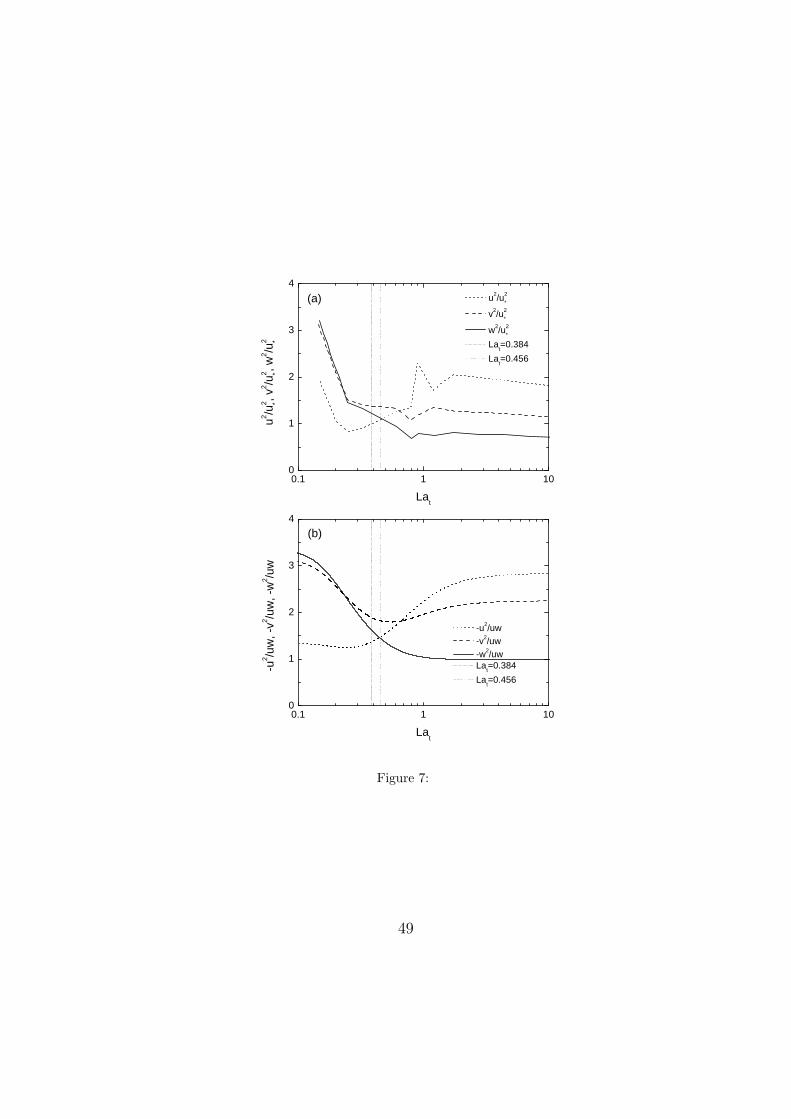
In Fig. 7a, Fig. 5 of Li et al. (2005) is reproduced. Fig. 7b shows

−u2/uw, −v2/uw and −w2/uw calculated with the present model and plot-

ted for β = 2 taking α as αmin defined above, as a function of Lat calculated

from (34). The qualitative agreement of the two figures is remarkable, with a

correct ordering of the velocity variances for shear turbulence and for Lang-

muir turbulence, and the values of Lat where the curves cross each other

predicted with great accuracy. The point where u2 = w2, in particular, can

be determined easily from (34), since from Fig. 3a, this should correspond

roughly to αmin = 1/2 and (u2/w2)min = 1. If these values are used, one ob-

tains a critical Lat (where the transition from shear turbulence to Langmuir

turbulence occurs according to this criterion) given by

(Lat)crit =(√

2e−1κ)1/2

. (35)

Using κ = 0.4, this is evaluated to be (Lat)crit = 0.456 and is plotted in Fig.

7 as the vertical dotted line. The agreement of this line with the point where

w2/u2 = 1 both in Fig. 7b (where α = αmin everywhere and thus where the

best agreement would be expected) and with Fig. 7a (where the conditions

are more complex) is remarkable. The vertical dashed line corresponds to the

same calculation if in (29) the full friction velocity was considered instead

of u∗s. This would amount to neglecting the factor inside square brackets

in (34) and the square-root of 2 in (35), giving instead (Lat)crit = 0.384.

32

Clearly, the larger value of (Lat)crit is more accurate than the smaller one,

emphasising the importance of partitioning the shear stress as in (30).

In other detailed features, the agreement of Figs. 7a and 7b is less satis-

factory. For example, the present model underestimates the increase of u2/u2∗

for low values of Lat and overestimates both u2/u2∗ and v2/u2

∗ for high Lat.

The difference between w2 and either u2 or v2 for high Lat is also too marked

(a well-known deficiency of RDT – see Townsend (1976)). But, given the

fact that the quantities plotted in Fig. 7a are averaged in the vertical, and

that the mean velocity profile varies vertically in a complicated way in the

LES of Li et al. (2005), the agreement is surprisingly good.

It is also noteworthy that no blocking effects of the air-water interface on

the turbulence have been taken into account in the calculations (cf. Teixeira

and Belcher, 2006, 2010). This is not too problematic, because the regions of

the flow where these effects are felt correspond to a negligible fraction of the

depth intervals used by Li et al. (2005) to compute the averages presented

in Fig. 7a. The method for relating Lat to α is, necessarily, one of the most

questionable aspects of the procedure outlined above, and obviously many

alternatives could be devised.

4. Conclusions

The structure of turbulence beneath surface water waves was investigated

theoretically using RDT. In the surface layer of the ocean, the turbulence is

dynamically affected essentially by two external forcings, which distort its

vorticity: the vertical gradient of the mean Eulerian current, and the vertical

gradient of the Stokes drift transport, associated with the surface waves.

33

The evolution of the turbulence energy, anisotropy and elongation due to

these two forcings was studied for initially isotropic turbulence through the

calculation of Reynolds stresses and integral length scales, and their ratios.

The parameter space was explored for situations with distortion by shear

only, by Stokes drift only (relevant to swell), by shear and a Stokes drift

gradient with the same sign (relevant to wind waves), and by shear and a

Stokes drift gradient of opposite signs (relevant to waves propagating against

the wind). The TKE grows algebraically for distortion by shear only or by

Stokes drift only, decays for shear and a Stokes drift gradient of opposite

signs, and grows exponentially for shear and a Stokes drift gradient with

the same sign. This is a manifestation of the linear instability mechanism

investigated by Craik and Leibovich (1976), which is included in the possible

modes of growth of disturbances in RDT. Craik and Leibovich’s linear in-

stability condition for Langmuir circulations in the inviscid and unstratified

limit was found to be formally equivalent to the linear instability condition

for a rotating shear flow, investigated by Bradshaw (1969), if the Eulerian

mean velocity is replaced by the Lagrangian mean velocity (including the

Stokes drift) and if the rotation rate is related to the gradient of the Stokes

drift in an appropriate way.

The anisotropy of the turbulence was found to range from that typical

of streaky structures (where the streamwise velocity fluctuations are domi-

nant and elongated in the streamwise direction) when only shear exists, to

that typical of streamwise vortices (where the spanwise and vertical velocity

fluctuations are dominant and elongated in the same direction) when only

the Stokes drift exists. When the shear and the Stokes drift gradient have

34

the same sign, the turbulence is highly energetic and more isotropic, with

all velocity fluctuations strongly elongated in the streamwise direction. It

apparently contains both streaky structures and streamwise vortices. On the

other hand, when the shear and the Stokes drift gradient have opposite signs,

the turbulence is weak, rather isotropic, and not elongated.

The fact that Langmuir circulations have often been observed, or simu-

lated numerically, with a structure close to that of pure streamwise vortices

suggests that the effect of the Stokes drift becomes dominant as the circu-

lations evolve. This is consistent with observations by Smith (1998), which

show that, in well-developed Langmuir circulations, the friction velocity no

longer enters directly in scaling the motion. This behaviour is probably due

to the suppression of the shear current by the strong vertical mixing asso-

ciated with the large vertical velocity variances that exist when 0 ≤ α < 1.

The experiments of Melville et al. (1998) support this view.

The turbulence structure produced by the present model in the parameter

range 0 < α < 1 is consistent with the structure of turbulence beneath water

waves in the experiments of Thais and Magnaudet (1996), and surprisingly

also with the structure of turbulence in atmospheric flows over undulating

terrain (Mason and King, 1984; Gong et al., 1996). In all of these cases, no

Langmuir circulations as usually defined were reported, but the turbulence

was more isotropic and energetic than in flat-wall boundary layers. The

comparison carried out with the LES data of Li et al. (2005) for u2/u2∗, v2/u2

∗

and w2/u2∗ as a function of Lat showed that the transition of the anisotropy

from shear turbulence to Langmuir turbulence is reproduced qualitatively

well by RDT. The value of Lat at which this transition occurs is also predicted

35

accurately.

All these results highlight the potential usefulness of RDT for develop-

ing physically-based parameterisations of turbulent processes in the oceanic

boundary layer.

Acknowledgements

I acknowledge the financial support of the Portuguese Science Foundation

(FCT) under Project AWARE/PTDC/CTE-ATM/65125/2006.

References

Andrews, D. G., McIntyre, M. E., 1978. An exact theory of nonlinear waves

on a Lagrangian-mean flow. Journal of Fluid Mechanics 89, 609–646.

Ardhuin, F., Jenkins, A. D., 2006. On the interaction of surface waves and

upper ocean turbulence. Journal of Physical Oceanography 36, 551–557.

Ardhuin, F., Marie, L., Rascle, N., Forget, P., Roland, A., 2009. Observation

and estimation of Lagrangian, Stokes, and Eulerian currents induced by

wind and waves at the sea surface. Journal of Physical Oceanography 39,

2820–2838.

Ardhuin, F., Rascle, N., Belibassakis, K. A., 2008. Explicit wave-averaged

primitive equations using a generalized Lagrangian mean. Ocean Modelling

20, 35–60.

Batchelor, G. K., Proudman, I., 1954. The effect of rapid distortion of a

fluid in turbulent motion. Quarterly Journal of Mechanics and Applied

Mathematics 7, 83–103.

36

Belcher, S. E., Harris, J. A., Street, R. L., 1994. Linear dynamics of wind

waves in coupled turbulent air-water flow. Part 1. Theory. Journal of Fluid

Mechanics 271, 119–151.

Bradshaw, P., 1969. The analogy between streamline curvature and buoyancy

in turbulent shear flow. Journal of Fluid Mechanics 36, 177–191.

Cambon, C., Benoit, J.-P., Shao, L., Jacquin, L., 1994. Stability analysis

and large-eddy simulation of rotating turbulence with organized eddies.

Journal of Fluid Mechanics 278, 175–200.

Cambon, C., Scott, J. F., 1999. Linear and nonlinear models of anisotropic

turbulence. Annual Review of Fluid Mechanics 31, 1–53.

Craik, A. D. D., 1977. The generation of Langmuir circulations by an insta-

bility mechanism. Journal of Fluid Mechanics 81, 209–223.

Craik, A. D. D., 1982. The generalized Lagrangian-mean equations and hy-

drodynamic stability. Journal of Fluid Mechanics 125, 27–35.

Craik, A. D. D., Leibovich, S., 1976. A rational model for Langmuir circula-

tions. Journal of Fluid Mechanics 73, 401–426.

D’Asaro, E., 2001. Turbulent vertical kinetic energy in the ocean mixed layer.

Journal of Physical Oceanography 31, 3530-3537.

Faller, A. J., Auer, S. J., 1988. The roles of Langmuir circulations in the

dispersion of surface tracers. Journal of Physical Oceanography 18, 1108–

1123.

37

Founda, D., Tombrou, M., Lalas, D. P., Asimakopoulos, D. N., 1997. Some

measurements of turbulence characteristics over complex terrain. Bound-

ary Layer Meteorology 83, 221–245.

Gartshore, I. S., Durbin, P. A., Hunt, J. C. R., 1983. The production of

turbulent stress in a shear flow by irrotational fluctuations. Journal of

Fluid Mechanics 137, 307–329.

Gong, W., Taylor, P. A., Dornbrack, A., 1996. Turbulent boundary-layer

flow over fixed aerodynamically rough two-dimensional sinusoidal waves.

Journal of Fluid Mechanics 312, 1–37.

Grant, A. L. M., Belcher, S. E., 2009. Characteristics of Langmuir turbulence

in the ocean mixed layer. Journal of Physical Oceanography 39, 1871–1887.

Hunt, J. C. R., 1984. Turbulence structure in thermal convection and shear-

free boundary layers. Journal of Fluid Mechanics 138, 161–184.

Hunt, J. C. R., Carruthers, D. J., 1990. Rapid distortion theory and the

‘problems’ of turbulence. Journal of Fluid Mechanics 212, 497–532.

Kantha, L., Wittmann, P., Sclavo, M., Carniel, S., 2009. A preliminary es-

timate of the Stokes dissipation of wave energy in the global ocean. Geo-

physical Research Letters 36, L02605.

Kevlahan, N. K.-R., Hunt, J. C. R., 1997. Nonlinear interactions in turbu-

lence with strong irrotational straining. Journal of Fluid Mechanics 337,

333–364.

38

Kline, S. J., Reynolds, W. C., Shraub, F. A., Runstadler, P. W., 1967. The

structure of turbulent boundary layers. Journal of Fluid Mechanics 30,

741–773.

Leblanc, S., Cambon, C., 1997. On the three-dimensional instabilities of

plane flows subjected to Coriolis force. Physics of Fluids 9, 1307–1316.

Lee, M. J., Kim, J., Moin, P., 1990. Structure of turbulence at high shear

rate. Journal of Fluid Mechanics 216, 561–583.

Leibovich, S., 1977. Convective instability of stably stratified water in the

ocean. Journal of Fluid Mechanics 82, 561–581.

Leibovich, S., 1980. On wave-current interaction theories of Langmuir circu-

lations. Journal of Fluid Mechanics 99, 715–724.

Leibovich, S., 1983. The form and dynamics of Langmuir circulations. Annual

Review of Fluid Mechanics 15, 391–427.

Li, M., Garrett, C., Skyllingstad, E., 2005. A regime diagram for classifying

turbulent large eddies in the upper ocean. Deep-Sea Research 52, 259–278.

Mann, J., 1994. The spatial structure of neutral atmospheric surface-layer

turbulence. Journal of Fluid Mechanics 273, 141–168.

Mason, P. J., King, J. C., 1984. Atmospheric flow over a succession of nearly

two-dimensional ridges and valleys. Quarterly Journal of the Royal Mete-

orological Society 110, 821–845.

McWilliams, J. C., Sullivan, P. P., Moeng, C.-H., 1997. Langmuir turbulence

in the ocean. Journal of Fluid Mechanics 334, 1–30.

39

Melville, W. K., Shear, R., Veron, F., 1998. Laboratory measurements of

the generation and evolution of Langmuir circulations. Journal of Fluid

Mechanics 364, 31–58.

Noh, Y., Min, H. S., Raasch, S., 2004. Large eddy simulation of the ocean

mixed layer: the effects of wave breaking and Langmuir circulation. Journal

of Physical Oceanography 34, 720–735.

Phillips, W. R. C., 2001. On the pseudomomentum and generalized Stokes

drift in a spectrum of rotational waves. Journal of Fluid Mechanics 430,

209–229.

Phillips, W. R. C., Wu, Z., 1994. On the instability of wave-catalysed longi-

tudinal vortices in strong shear. Journal of Fluid Mechanics 272, 235–254.

Phillips, W. R. C., Wu, Z., Lumley, J. L., 1996. On the formation of longi-

tudinal vortices in a turbulent boundary layer over wavy terrain. Journal

of Fluid Mechanics 326, 321–341.

Polton, J. A., Belcher, S. E., 2007. Langmuir turbulence and deeply pene-

trating jets in an unstratified mixed layer. Journal of Geophysical Research

112, C09020.

Rascle, N., Ardhuin, F., Terray, E. A., 2006. Drift and mixing under the

ocean surface: A coherent one-dimensional description with application to

unstratified conditions. Journal of Geophysical Research 111, C03016.

Salhi, A., Cambon, C., 1997. An analysis of rotating shear flow using linear

theory and DNS and LES results. Journal of Fluid Mechanics 347, 171–195.

40

Savill, A. M., 1987. Recent developments in rapid-distortion theory. Annual

Review of Fluid Mechanics 19, 531–575.

Shrira, V. I., 1993. Surface waves on shear currents: solution of the boundary-

value problem. Journal of Fluid Mechanics 252, 565–584.

Smith, J. A., 1998. Evolution of Langmuir circulation during a storm. Journal

of Geophysical Research 103, 12649–12668.

Speziale, C. G., Abid, R., Blaisdell, G. A., 1996. On the consistency of

Reynolds stress turbulence closures with hydrodynamic stability theory.

Physics of Fluids 8, 781–788.

Speziale, C. G., MacGiolla Mhuiris, N., 1989. On the prediction of equilib-

rium states in homogeneous turbulence. Journal of Fluid Mechanics 209,

591–615.

Teixeira, M. A. C., Belcher, S. E., 2000. Dissipation of shear-free turbulence

near boundaries. Journal of Fluid Mechanics 422, 167–191.

Teixeira, M. A. C., Belcher, S. E., 2002. On the distortion of turbulence by

a progressive surface wave. Journal of Fluid Mechanics 458, 229–267.

Teixeira, M. A. C., Belcher, S. E., 2006. On the initiation of surface waves

by turbulent shear flow. Dynamics of Atmospheres and Oceans 41, 1–27.

Teixeira, M. A. C., Belcher, S. E., 2010. On the structure of Langmuir tur-

bulence. Ocean Modelling 31, 105–119.

Thais, L., Magnaudet, J., 1996. Turbulent structure beneath surface gravity

waves sheared by the wind. Journal of Fluid Mechanics 328, 313–344.

41

Townsend, A. A., 1970. Entrainment and the structure of turbulent flow.

Journal of Fluid Mechanics 41, 13–46.

Townsend, A. A., 1976. The structure of turbulent shear flow. Cambridge

University Press.

42

=2

L

US

U

=−1α α =0 α =1 α

U

Figure 1:

43

0

0.5

1

α

0 2 4 6 8 10

β

-1

-0.5

0

(a)

1

1.5

2

0

0.5

1

α

0 2 4 6 8 10

β

-1

-0.5

0

(b)

1

1.5

2

0

0.5

1

α

0 2 4 6 8 10

β

-1

-0.5

0

(c)

1

1.5

2

0

0.5

1

α

0 2 4 6 8 10

β

-1

-0.5

0

(d)

1

1.5

2

0

0.5

1

α

0 2 4 6 8 10

β

-1

-0.5

0

(e)

1

1.5

2

Figure 2:

44

0

0.5

1

α

0 2 4 6 8 10

β

-1

-0.5

0

(a)

1

1.5

2

0

0.5

1

α

0 2 4 6 8 10

β

-1

-0.5

0

(b)

1

1.5

2

0

0.5

1

α

0 2 4 6 8 10

β

-1

-0.5

0

(c)

1

1.5

2

0

0.5

1

α

0 2 4 6 8 10

β

-1

-0.5

0

(d)

1

1.5

2

Figure 3:

45

0

0.5

1

α

0 2 4 6 8 10

β

-1

-0.5

0

(a)

1

1.5

2

0

0.5

1

α

(b)

1

1.5

2

0 2 4 6 8 10

β

-1

-0.5

0

0

0.5

1

α

0 2 4 6 8 10

β

-1

-0.5

0

(c)

1

1.5

2

0

0.5

1

α

0 2 4 6 8 10

β

-1

-0.5

0

(d)

1

1.5

2

0

0.5

1

α

0 2 4 6 8 10

β

-1

-0.5

0

(e)

1

1.5

2

0

0.5

1

α

0 2 4 6 8 10

β

-1

-0.5

0

(f)

1

1.5

2

Figure 4:

46

0

0.5

1

α

0 2 4 6 8 10

β

-1

-0.5

0

(a)

1

1.5

2

0

0.5

1

α

0 2 4 6 8 10

β

-1

-0.5

0

(b)

1

1.5

2

0

0.5

1

α

0 2 4 6 8 10

β

-1

-0.5

0

(c)

1

1.5

2

Figure 5:

47

0 1 2 3 4 5 60

1

2

3

4

5

6

7

8

R=-1 R=-1/2 R=0 R=1 α=0 α=1/2 α=1 α=2

K/K

0

β

(a)

-1.0 -0.5 0.0 0.5 1.0 1.5 2.00

2

4

6

8

10

K/K

0

α

(b)

-2.0 -1.5 -1.0 -0.5 0.0 0.5 1.0

R

0 1 2 3 4 50

1

2

3

4

5

6

7

8

9

10

R=-3/2 R=-1 R=-1/2 R=0 R=1/2 α=-1/2 α=0 α=1/2 α=1 α=3/2

Lx 11/(

2Ly 11

)

β

(c)

Figure 6:

48

0.1 1 100

1

2

3

4 u2/u2

*

v2/u2

*

w2/u2

*

Lat=0.384

Lat=0.456

u2 /u

2 *, v2 /u

2 *, w2 /u

2 *

Lat

(a)

0.1 1 100

1

2

3

4

-u2/uw -v2/uw -w2/uw La

t=0.384

Lat=0.456

-u2 /u

w, -

v2 /uw

, -w

2 /uw

Lat

(b)

Figure 7:

49

Figure captions

Figure 1: Diagram showing schematic profiles of the vertical gradient of the

total Lagrangian transport, dUL/dz (assumed to be constant), of the vertical

gradient of the Eulerian velocity, dU/dz, and of the vertical gradient of the

Stokes drift transport, dUS/dz, for the range of α considered in the present

study.

Figure 2: Reynolds stresses normalised by the initial RMS velocity, q, as a

function of α and β. (a) streamwise velocity variance, u2/q2, (b) spanwise

velocity variance, v2/q2, (c) vertical velocity variance, w2/q2, (d) turbulent

kinetic energy, K/q2, (e) shear stress, uw/q2.

Figure 3: Ratios of the Reynolds stresses, as a function of α and β. (a)

vertical to streamwise velocity variance, w2/u2, (b) vertical to spanwise ve-

locity variance, w2/v2, (c) spanwise to streamwise velocity variance, v2/u2,

(d) minus the shear stress to TKE, −uw/K.

Figure 4: Integral length scales normalised by the initial longitudinal length

scale, l, as a function of α and β. (a) Lx11/l, (b) Ly

11/l, (c) Lx22/l, (d) Ly

22/l,

(e) Lx33/l, (f) Ly

33/l.

Figure 5: Ratios of the integral length scales in the streamwise (x) and in the

spanwise (y) directions as a function of α and β. (a) Lx11/L

y11, (b) Lx

22/Ly22,

(c) Lx33/L

y33.

Figure 6: Comparison between results from the present model (lines) and

from inviscid RDT calculations of turbulence in a rotating shear flow by

50

Cambon et al. (1994) and Salhi and Cambon (1997) (symbols). (a) Nor-

malised TKE, K/K0, as a function of β. (b) Normalised TKE as a function

of α (or R). (c) Lx11/(2L

y11) as a function of β.

Figure 7: Velocity variances normalised by the friction velocity (u2/u2∗, v2/u2

∗

and w2/u2∗) or by the shear stress (−u2/uw, −v2/uw and −w2/uw) as a

function of Lat. (a) Results from Fig. 5 of Li et al. (2005). (b) Results from

the present model at β = 2 and with Lat estimated from (34). The vertical

lines predict the value of Lat at which w2/u2 = 1.

51