a linearized free-surface method for prediction of unsteady ship
TRANSCRIPT
A Linearized Free-Surface Method for Predictionof Unsteady Ship Maneuvering
by
Marc O. Woolliscroft
A dissertation submitted in partial fulfillmentof the requirements for the degree of
Doctor of Philosophy(Naval Architecture and Marine Engineering)
in The University of Michigan2015
Doctoral Committee:
Assistant Professor Kevin J. Maki, ChairAssistant Professor Matthew D. ColletteAssistant Professor Eric JohnsenProfessor Armin W. Troesch

“Experience: that most brutal of teachers. But you learn, my God do you learn.”
-C. S. Lewis

c© Marc O. Woolliscroft 2015
All Rights Reserved

Dedicated to my family
ii
ACKNOWLEDGEMENTS
Without doubt, this thesis is not solely a display of individual accomplishment. The
presence of several people in my life motivate the production of this work in unique
ways. I thank my advisor, Dr. Kevin Maki, for his continued support and patience
throughout the course of my research. His ability to not only teach but also befriend
I highly commend. I will appreciate his mentorship for my entire career. Dr. Armin
Troesch and Dr. Matthew Collette provide me with invaluable knowledge and expe-
riences through classes and conferences in addition to my doctoral work. Dr. Eric
Johnsen is beneficial in offering a perspective outside the realm of naval architecture
and marine engineering. I am a stronger student and engineering because of my
committee members.
I would like to gratefully acknowledge Kelly Cooper of the U.S. Office of Naval Re-
search and administer of program number N00014-13-1-0759 for providing funding for
my education. Additional acknowledgment goes to the Flux HPC Cluster provided by
the University of Michigan Office of Research and operated by the High Performance
Computing Group at the College of Engineering. Travel funds for participation in
an international workshop are kindly provided by the Rackham Graduate School.
Also, thanks to the team at Engys for offering technical advice and consulting at the
beginning stages of my thesis work.
My academic career is not possible without the support from my family, girlfriend,
and friends who always encouraged me and provided me with refreshing distractions
when a break from work was necessary. I am in debt to the friends that remain in
iii

contact when I am less prone to do so. Most importantly, my parents, James and
Elizabeth, show neverending love and support for me in all my endeavors. To all of
you, please do not underestimate my gratitude.
iv
TABLE OF CONTENTS
DEDICATION . . . . . . . . . . . . . . . . . . . . . . . . . . . . . . . . . . ii
ACKNOWLEDGEMENTS . . . . . . . . . . . . . . . . . . . . . . . . . . iii
LIST OF FIGURES . . . . . . . . . . . . . . . . . . . . . . . . . . . . . . . vii
LIST OF TABLES . . . . . . . . . . . . . . . . . . . . . . . . . . . . . . . . ix
ABSTRACT . . . . . . . . . . . . . . . . . . . . . . . . . . . . . . . . . . . x
CHAPTER
I. Introduction . . . . . . . . . . . . . . . . . . . . . . . . . . . . . . 1
1.1 Definition of Maneuvering . . . . . . . . . . . . . . . . . . . . 41.2 Design for Maneuverability . . . . . . . . . . . . . . . . . . . 5
II. Background . . . . . . . . . . . . . . . . . . . . . . . . . . . . . . . 10
2.1 Maneuvering Prediction Methods . . . . . . . . . . . . . . . . 102.1.1 Experiments . . . . . . . . . . . . . . . . . . . . . . 122.1.2 Numerical Simulations . . . . . . . . . . . . . . . . 152.1.3 Summary . . . . . . . . . . . . . . . . . . . . . . . . 18
III. Free-Surface Boundary Conditions . . . . . . . . . . . . . . . . 20
3.1 The Air-Water Interface . . . . . . . . . . . . . . . . . . . . . 203.2 Nonlinear Free-Surface Boundary Conditions . . . . . . . . . 223.3 Linearized Free-Surface Boundary Conditions . . . . . . . . . 25
IV. Linearized Free-Surface Solver . . . . . . . . . . . . . . . . . . . 33
4.1 ALE Formulation . . . . . . . . . . . . . . . . . . . . . . . . 334.2 Boundary Condition at Free-Surface/Body Juncture . . . . . 35
v
4.3 Numerical Aspects . . . . . . . . . . . . . . . . . . . . . . . . 374.4 KCS Validation . . . . . . . . . . . . . . . . . . . . . . . . . . 39
V. Viscous Air-Water Interface Study . . . . . . . . . . . . . . . . 43
5.1 Canonical Viscous Interface Study . . . . . . . . . . . . . . . 435.1.1 VOF Numerical Method . . . . . . . . . . . . . . . 445.1.2 Description of Canonical Problem . . . . . . . . . . 46
5.2 Results . . . . . . . . . . . . . . . . . . . . . . . . . . . . . . 495.2.1 FrT = 3 – Steady Wave . . . . . . . . . . . . . . . . 515.2.2 FrT = 2 – Unsteady Breaking Wave . . . . . . . . . 625.2.3 FrT = 0.2 – Low Froude Number Regime . . . . . . 71
5.3 Summary of Findings . . . . . . . . . . . . . . . . . . . . . . 77
VI. Maneuvering Tests . . . . . . . . . . . . . . . . . . . . . . . . . . 80
6.1 DTMB 5415 - Bare Hull . . . . . . . . . . . . . . . . . . . . . 816.1.1 Static Drift . . . . . . . . . . . . . . . . . . . . . . . 846.1.2 Pure Sway . . . . . . . . . . . . . . . . . . . . . . . 896.1.3 Pure Yaw . . . . . . . . . . . . . . . . . . . . . . . . 926.1.4 CPU Requirements . . . . . . . . . . . . . . . . . . 956.1.5 Flow Field Data . . . . . . . . . . . . . . . . . . . . 96
6.2 DTMB 5415M - Appended Hull . . . . . . . . . . . . . . . . 103
VII. Conclusions and Future Work . . . . . . . . . . . . . . . . . . . 109
7.1 Summary . . . . . . . . . . . . . . . . . . . . . . . . . . . . . 1097.2 Contributions . . . . . . . . . . . . . . . . . . . . . . . . . . . 1117.3 Future Work . . . . . . . . . . . . . . . . . . . . . . . . . . . 112
APPENDIX . . . . . . . . . . . . . . . . . . . . . . . . . . . . . . . . . . . . 115
BIBLIOGRAPHY . . . . . . . . . . . . . . . . . . . . . . . . . . . . . . . . 126
vi
LIST OF FIGURES
Figure
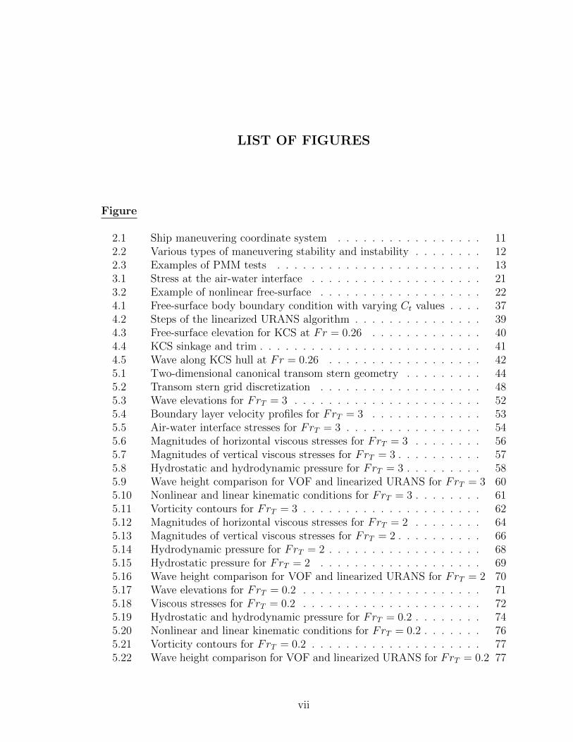
2.1 Ship maneuvering coordinate system . . . . . . . . . . . . . . . . . 112.2 Various types of maneuvering stability and instability . . . . . . . . 122.3 Examples of PMM tests . . . . . . . . . . . . . . . . . . . . . . . . 133.1 Stress at the air-water interface . . . . . . . . . . . . . . . . . . . . 213.2 Example of nonlinear free-surface . . . . . . . . . . . . . . . . . . . 224.1 Free-surface body boundary condition with varying Ct values . . . . 374.2 Steps of the linearized URANS algorithm . . . . . . . . . . . . . . . 394.3 Free-surface elevation for KCS at Fr = 0.26 . . . . . . . . . . . . . 404.4 KCS sinkage and trim . . . . . . . . . . . . . . . . . . . . . . . . . . 414.5 Wave along KCS hull at Fr = 0.26 . . . . . . . . . . . . . . . . . . 425.1 Two-dimensional canonical transom stern geometry . . . . . . . . . 445.2 Transom stern grid discretization . . . . . . . . . . . . . . . . . . . 485.3 Wave elevations for FrT = 3 . . . . . . . . . . . . . . . . . . . . . . 525.4 Boundary layer velocity profiles for FrT = 3 . . . . . . . . . . . . . 535.5 Air-water interface stresses for FrT = 3 . . . . . . . . . . . . . . . . 545.6 Magnitudes of horizontal viscous stresses for FrT = 3 . . . . . . . . 565.7 Magnitudes of vertical viscous stresses for FrT = 3 . . . . . . . . . . 575.8 Hydrostatic and hydrodynamic pressure for FrT = 3 . . . . . . . . . 585.9 Wave height comparison for VOF and linearized URANS for FrT = 3 605.10 Nonlinear and linear kinematic conditions for FrT = 3 . . . . . . . . 615.11 Vorticity contours for FrT = 3 . . . . . . . . . . . . . . . . . . . . . 625.12 Magnitudes of horizontal viscous stresses for FrT = 2 . . . . . . . . 645.13 Magnitudes of vertical viscous stresses for FrT = 2 . . . . . . . . . . 665.14 Hydrodynamic pressure for FrT = 2 . . . . . . . . . . . . . . . . . . 685.15 Hydrostatic pressure for FrT = 2 . . . . . . . . . . . . . . . . . . . 695.16 Wave height comparison for VOF and linearized URANS for FrT = 2 705.17 Wave elevations for FrT = 0.2 . . . . . . . . . . . . . . . . . . . . . 715.18 Viscous stresses for FrT = 0.2 . . . . . . . . . . . . . . . . . . . . . 725.19 Hydrostatic and hydrodynamic pressure for FrT = 0.2 . . . . . . . . 745.20 Nonlinear and linear kinematic conditions for FrT = 0.2 . . . . . . . 765.21 Vorticity contours for FrT = 0.2 . . . . . . . . . . . . . . . . . . . . 775.22 Wave height comparison for VOF and linearized URANS for FrT = 0.2 77
vii

6.1 IIHR DTMB 5415 bare hull model . . . . . . . . . . . . . . . . . . . 826.2 FORCE DTMB 5415 bare hull model . . . . . . . . . . . . . . . . . 826.3 Grid convergence study for linearized URANS static drift . . . . . . 866.4 Force and moment uncertainties for linearized URANS static drift . 876.5 Pressure comparison for linearized URANS and double-body . . . . 886.6 Forces and moments for linearized URANS and double-body . . . . 896.7 Forces and moment for pure sway compared to IIHR data . . . . . . 916.8 Forces and moment for pure sway compared to FORCE data . . . . 926.9 Forces and moment for pure yaw compared to IIHR data . . . . . . 936.10 Forces and moment for pure yaw compared to FORCE data . . . . 956.11 PIV sampling points and locations for pure sway . . . . . . . . . . . 976.12 Axial velocity contour plots . . . . . . . . . . . . . . . . . . . . . . 986.13 Lateral velocity contour plots . . . . . . . . . . . . . . . . . . . . . 996.14 Vertical velocity contour plots . . . . . . . . . . . . . . . . . . . . . 1006.15 Axial vorticity contour plots . . . . . . . . . . . . . . . . . . . . . . 1016.16 Turbulent kinetic energy contour plots . . . . . . . . . . . . . . . . 1026.17 MARIN DTMB 5415M appended hull model . . . . . . . . . . . . . 1036.18 Coarse grid discretization of the DTMB 5415M stern region . . . . . 1046.19 Force and moment for static drift compared to MARIN data . . . . 1066.20 Mean propeller thrust for static drift . . . . . . . . . . . . . . . . . 1076.21 Propeller thrust time series for static drift . . . . . . . . . . . . . . 1076.22 Propeller thrust for two rotations showing thrust impulses . . . . . 108A.1 Magnitudes of horizontal viscous stresses for FrT = 2, Re = 1e5 . . 118A.2 Magnitudes of vertical viscous stresses for FrT = 2, Re = 1e5 . . . . 119A.3 Hydrodynamic pressure for FrT = 2, Re = 1e5 . . . . . . . . . . . . 120A.4 Hydrostatic pressure for FrT = 2, Re = 1e5 . . . . . . . . . . . . . 121A.5 Magnitudes of horizontal viscous stresses for FrT = 2, Re = 1e6 . . 122A.6 Magnitudes of vertical viscous stresses for FrT = 2, Re = 1e6 . . . . 123A.7 Hydrodynamic pressure for FrT = 2, Re = 1e6 . . . . . . . . . . . . 124A.8 Hydrostatic pressure for FrT = 2, Re = 1e6 . . . . . . . . . . . . . 125
viii
LIST OF TABLES
Table
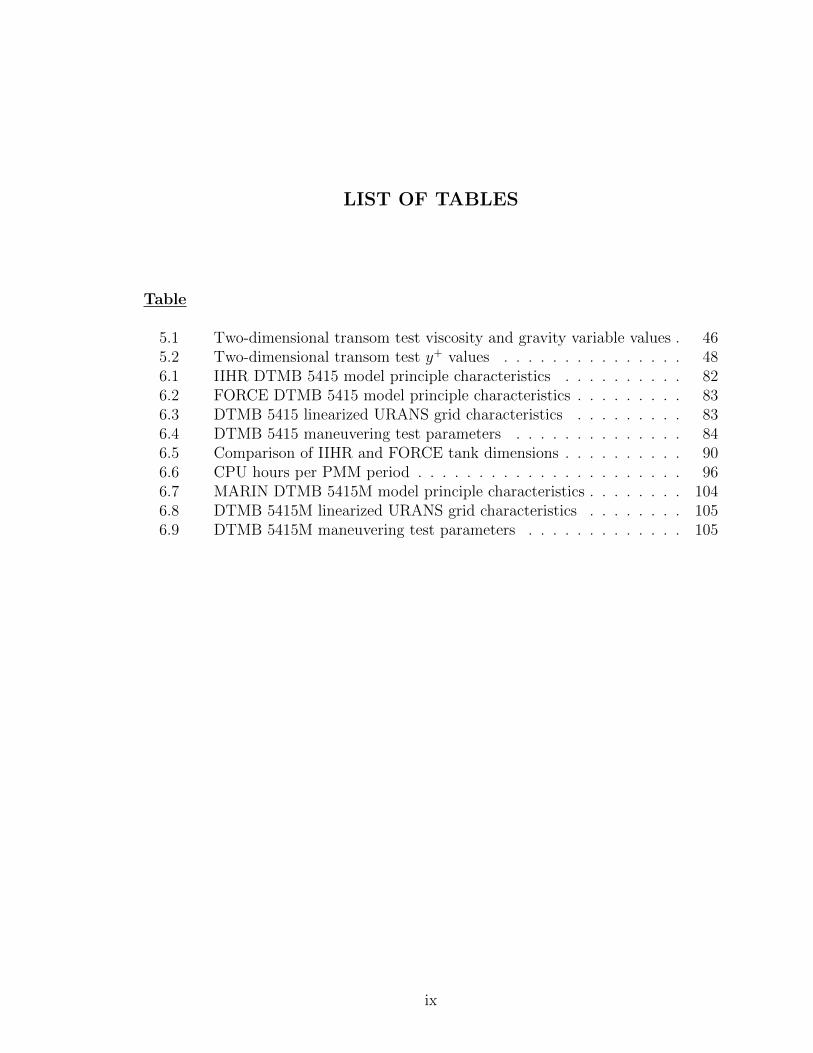
5.1 Two-dimensional transom test viscosity and gravity variable values . 465.2 Two-dimensional transom test y+ values . . . . . . . . . . . . . . . 486.1 IIHR DTMB 5415 model principle characteristics . . . . . . . . . . 826.2 FORCE DTMB 5415 model principle characteristics . . . . . . . . . 836.3 DTMB 5415 linearized URANS grid characteristics . . . . . . . . . 836.4 DTMB 5415 maneuvering test parameters . . . . . . . . . . . . . . 846.5 Comparison of IIHR and FORCE tank dimensions . . . . . . . . . . 906.6 CPU hours per PMM period . . . . . . . . . . . . . . . . . . . . . . 966.7 MARIN DTMB 5415M model principle characteristics . . . . . . . . 1046.8 DTMB 5415M linearized URANS grid characteristics . . . . . . . . 1056.9 DTMB 5415M maneuvering test parameters . . . . . . . . . . . . . 105
ix

ABSTRACT
A Linearized Free-Surface Method for Prediction of Unsteady Ship Maneuvering
by
Marc O. Woolliscroft
Chair: Kevin J. Maki
Maneuvering prediction tools are valuable resources for naval and commercial ship
designers. They estimate the ability of a ship to maintain or alter course. This en-
ables designers to characterize the maneuvering performance of multiple conceptual
hull forms and select an optimal design. A novel maneuvering prediction method is
presented in this thesis. It is an unsteady Reynolds-averaged Navier-Stokes (URANS)
approach that includes wave effects with linear free-surface boundary conditions.
Therefore, it is a single-phase approach to solving multiphase problems. The so-
lution of the URANS equations captures the viscous effects that are highly important
in maneuvering due to the complex fluid interactions between the hull, propellers,
and rudders. The linearized free-surface approximation accounts for first-order wave
effects while reducing the necessary extents of the computational domain and the level
of grid refinement required by nonlinear computational fluid dynamics (CFD) solvers.
These simplifications lead to a substantial improvement in computational efficiency
with respect to nonlinear methods, while retaining accuracy and empowering naval
architects to obtain results earlier in the design cycle.
x
CHAPTER I
Introduction
Naval architects find balanced solutions between the main drivers in ship design.
Speed, weight, space, and cost are routinely of the utmost concern. Primarily gov-
erned by the need to displace enough water in relation to the ship mass in order to
float, the study of ship design uncovers a great deal of connectedness between these
core drivers. Rarely is there an improvement in one area without adversely effecting
another area to some degree. For example, new composite materials pose a great
opportunity for savings in weight while maintaining high strength properties. There-
fore, they can be ideal for high-speed applications. However, they are more expensive
than traditional materials and require different methods of fabrication. In another
case, it may be suggested that a smaller ship is generally less expensive to construct,
but this obviously limits the amount of cargo that may be transported and is in
contradiction with fundamental goals of commercial shipping companies. Also, naval
warships can be made with thick steel plating to survive damage incurred in battles,
yet this increases the weight of the ship which decreases the speed or increases fuel
consumption. This may be overcome with a higher capacity powering system, but
this in turn may require additional space and again increase weight. Clearly, ship de-
sign is a challenging problem. The inter-dependency of the engineering areas within
the overall design causes a change in one area to propagate and require consideration
1
for subsequent changes in several other areas. It is the duty of naval architects to
understand these connections and satisfy the requirements issued by ship owners for
new vessel designs.
Maneuvering plays a large role within the highly-connected areas of ship design.
Interactions between water, appendages, and control surfaces are not trivial. The
boundary layer present on a hull as it moves through water accounts for a large
viscous drag force. In addition, viscous separation can be generated from chines
or sonar domes during maneuvering. Violent and chaotic flow features exist such
as propeller cavitation and turbulence from appendages. Such widely varied flow
features can be present near the transom where the most important appendages for
maneuvering - rudders, propellers, skegs, et cetera - are located. Designing these
control surfaces requires consideration of the effects they have on course-keeping, fuel
efficiency, signatures, and so on. Making the proper design decisions is important
because the maneuverability of a vessel has direct effects on safety and performance.
For instance, a dynamically unstable ship needs proper skegs and rudders for frequent
course-checking. However, large skegs and frequent use of the rudders has a negative
impact on fuel consumption. On the other hand, a vessel which is too stable can not
turn within a reasonable distance. The ability to operate in specific ports throughout
the world requires various levels of maneuverability. Similarly, certain operations such
as ship-to-ship replenishment and canal navigation necessitate a high level of vessel
control. And furthermore, emergency situations need to be considered, and it must
be demonstrated that a ship can adequately change direction and stop to help avoid
catastrophic events.
However, these requirements create conflicting goals. Simple desires such as a
low hull resistance and the ability to stop quickly do not necessarily go hand-in-hand.
This leads to a design space containing conceptual hull forms, each of which satisfy the
design requirements to various degrees. The goal of a naval architect is to evaluate the
2
trade offs within the design space and deliver an optimal solution. Nevertheless, real-
world constraints such as schedules and budgets often result in a partial exploration
of novel hull forms. These design ideas resonate with those of set-based design, as
opposed to point-based design, discussed in Singer et al. (2009). Typically, historical
hull forms are used as a starting point. On one hand, it may be argued that an
existing hull can fully satisfy the requirements of a new design, but this approach
lacks a motivated effort to evolve the designs of the largest transportation vehicles in
the world. It simply does not push designs toward an optimized form. But, this is
not to suggest that high fidelity technologies are not available.
Surely, computational fluid dynamics (CFD) and structural finite-element meth-
ods (FEM) exist and are in use from time-to-time for design analysis. Even the
highly-important problem of arrangements on warships is the focus of early-stage
optimization efforts (Parsons et al., 2008; Gillespie, 2012). However, these tools can
be difficult to use requiring specially-skilled and well-trained designers. At times,
expensive licensing fees are associated with the use of high fidelity design software.
In addition, structural and fluid dynamics simulations can be very time-consuming.
These are all factors which limit the wide-spread use of such advanced tools. Still, on
rare occasions, a more original design may be pursued using high fidelity hydrody-
namic methods, but determining the maneuvering characteristics with these methods
is a difficult task.
Currently, maneuvering prediction capabilities consist of geometrically scaled model
tests and a variety of numerical methods. Model tests can provide a plethora of data,
helpful for studying ship motions as well as fluid dynamics, but they require expensive
facilities, models, and instruments, as well as methods to account for scaling effects
(Cope, 2012; Ueno et al., 2014). Numerical methods vary from inviscid potential
flow codes to multiphase CFD. Historically, the velocity potential framework pro-
vides solutions to several ship-motions problems, ranging from stability assessment
3
to the overtaking of one ship by another (Sclavounos and Thomas, 2007; Newman and
Tuck, 1974). But potential flow codes inherently lack the ability to capture viscous
separation, which is especially significant near the hull appendages that influence
maneuverability. Viscosity can not be ignored in complex, fully-inclusive simula-
tions involving rotating propellers moving a hull through a real fluid. On the other
hand, CFD and model tests can be used to obtain viscous predictions on hulls with
appendages (Broglia et al., 2013). However, these are costly and time-consuming.
Most designers do not have the computational resources necessary for unsteady CFD
simulations. Systems-based methods use equation-of-motion coefficients that have
been obtained from physical experiments or CFD to predict maneuvering capabili-
ties. These coefficients become less accurate with large motions or with changes in
hull geometry.
The main drawbacks of the existing technologies make them limited for hull form
optimization in early stages of design. Therefore, it is an important endeavor to
provide efficient and accurate tools that allow for a broad exploration of the design
space and the ability to develop more optimized designs within realistic time and
monetary constraints. A maneuvering prediction tool is presented in this thesis to
achieve this goal, but first it is necessary to define the important aspects of the ship
maneuvering problem.
1.1 Definition of Maneuvering
Maneuvering may be defined as ship motions caused by the interaction between water
and all surfaces of a vessel with which it is in contact. It is important to note just
how many surfaces this may include; the hull, bilge keels, rudders, stabilizer fins,
propellers, skegs, exposed struts and shafts, bulbous bows, gondolas, and all other
underwater appendages that interact with the water. Indeed, many of these surfaces
have been developed for the exact purpose of dictating maneuvering characteristics.
4
Termed control surfaces, these may be passive, as with skegs, or active, as with
rudders. Typical maneuvers include turning, stopping, and docking.
Maneuvering consists of low frequency ship motions usually requiringO (10− 100)
seconds and O (1− 10) ship lengths, L, to perform. Other scales to consider include
oncoming waves occurring with frequencies corresponding to O (10) seconds and pro-
peller rotations every O (1) second with blade-passings occurring more frequently.
Scales of O (0.01) seconds and smaller are needed to describe turbulence. Overall,
waves and other environmental factors affect maneuvering, but motions associated
with maneuvering occur at lower frequencies than oncoming waves, making it very
different than the study of seakeeping.
1.2 Design for Maneuverability
Upon receiving owner requirements for a novel ship design, maneuverists within a
design team have several options available to begin analyzing hull forms. Unlike
airplanes or automobiles, ships are unique because full-scale prototypes are infeasible
due to the enormous cost and time associated with constructing entire ships. This
leads one to consider a more reasonable approach; one in which a hull is scaled
to a smaller size. Geometrically scaled models let designers use towing tanks and
maneuvering basins to characterize hull forms in a physical setting. Here, they can
prescribe trajectories, many of which are not even possible at full scale, in order
to obtain very specific information about the hydrodynamic forces present during
maneuvering.
A high-fidelity alternative to model testing is fully nonlinear, multiphase CFD. In
this digital setting, designers are not limited by testing facilities or machining tools,
so meshes for multiple hulls may be tested simultaneously. Obviously, this is instead
limited by the computing resources available to the designers. A patent benefit of
numerical simulations is the possibility to perform analyses at a full scale Reynolds
5
number. These are not yet common, but obtaining solutions to full scale problems
while avoiding full scale construction holds great potential value.
Clearly, both physical experiments and nonlinear CFD simulations are important
tools for the study of ship maneuvering. They have been developed and improved
upon for decades, and they will remain widely-used in the future. However, the use
of these approaches comes with difficulties that can not be denied; difficulties that
hinder the idea of designing for maneuverability.
The Maritime Research Institute Netherlands (MARIN) reports constructing 150
models during the 2009 calender year using a CNC milling device which can be op-
erated 24 hours a day (de Boer, 2009). The year prior, Strock and Brown (2008)
use the U.S. Navy Advanced Ship and Submarine Evaluation Tool (ASSET) to gen-
erate 8,841 conceptual designs of a ballistic missile defense cruiser. ASSET is a
multi-platform design tool offering modules such as hull form, structures, resistance,
propulsion, machinery, weight, and spaces; but not maneuvering. Of the 8,841 de-
signs, 156 are “non-dominated,” or unique designs which should be explored further
and compared to determine strengths and weaknesses. Also in 2008, a nonlinear CFD
simulation of a bare hull 5415 model takes approximately 320 CPU hours to simulate
a 7.5 second maneuver (Miller, 2008). If the same computation is applied to the 156
non-dominated designs, nearly 50,000 CPU hours are required, and this ignores time
required for meshing, data transfer, post-processing, et cetera.
Undoubtedly, there is space for improvement. Tools such as ASSET make it pos-
sible to generate thousands of designs and truly explore a design space for optimized
solutions. However, state-of-the-art research centers such as MARIN and nonlinear
CFD simulations can not be used extensively at this stage. ASSET does provide
resistance estimation, but it is from the Holtrop-Mennen regression-based method
(Holtrop and Mennen, 1978, 1982). Certainly, the novel designs being generated may
differ greatly from the data used to construct the regression. Therefore, an oppor-
6

tunity exists for the development of efficient physics-based maneuvering prediction
methods that can be used in early stages of design.
The ability of a vessel to adequately stop, change direction, and maintain course is
key to performance and safety. Navigating through the entrances of ports may require
a specific path to avoid obstructions and other vessels. In a more extreme situation,
a drastic change in direction and speed may be necessary to prevent a catastrophic
collision. Ship size and operating requirements help dictate desired maneuvering char-
acteristics. Therefore, qualifications of ideal maneuverability differ between vessels
with different purposes. For example, a small patrol boat may actually be designed
to have low stability characteristics that allow for increased agility. In addition to
intended purpose, environmental factors such as water depth, channels, waves, and
currents influence maneuverability (Lincoln et al., 1989). The combination of these
factors and conflicting operational requirements make designing vessels for maneu-
verability a truly complex problem.
In addition to owner requirements, regulatory bodies drive the design for partic-
ular maneuvering qualities. Due to the need for a certain level of low frequency ship
motion control, the International Maritime Organization (IMO) has developed ma-
neuvering requirements for vessels over 100 meters in length. Requirements consist
of turning circle, zig-zag, and crashback (stopping) tests which are intended to mea-
sure course-keeping, course-changing, and stopping abilities (IMO, 2002). The vessel
length and speed are often used as criteria to determine if these have been completed
satisfactorily. For instance, the diameter of a turning circle must be less than five
ship lengths.
Furthermore, the American Bureau of Shipping (ABS) classification society, re-
quires that vessels demonstrate the ability to successfully perform these IMO ma-
neuvers during sea trials (ABS, 2006). The standards allow owners to conduct the
maneuvers in a condition other than full load only if predictive maneuvering analysis
7

has been performed at the design stage and deemed satisfactory. If trials are under-
gone in a condition other than full load, the results must agree with those obtained
with predictions. It is then assumed that the full load condition will agree with the
full load condition from the design stage. If predictions are not available, the sea
trials must be performed at the full load condition (Belenky and Falzarano, 2006).
Generally, this is not achievable due to the volume and expense of cargo that needs
to be on board, so maneuvering prediction during the design stage is almost always
necessary. Regardless, attempting to fulfill IMO maneuvering requirements only dur-
ing the full scale sea trials comes with great risk as this can lead to unsatisfactory
results causing costly hull form modifications, especially for novel designs that lack
historical data.
The linearized URANS method provides the ability for physics-based maneuvering
predictions in earlier design stages than nonlinear CFD or model tests. It relies on
first principles of free-surface boundary conditions as a basis for this novel approach.
The free-surface boundary conditions are considered in the classical linearized form,
but developed under the RANS variables for a viscous, turbulent fluid. Other state-
of-the-art technologies such as semi-automatic mesh generation, turbulence modeling,
and sliding mesh interfaces are coupled with this idea for an efficient and accurate
design solution to maneuvering prediction.
The development of the linearized URANS method herein primarily concerns ship
maneuvering problems from an inertial, Earth-fixed frame of reference. Forces and
moments are of the highest importance, but flow field information is also discussed.
In Chapter II, current state-of-the-art solutions to maneuvering problems are dis-
cussed. A theoretical presentation of the fully nonlinear free-surface boundary con-
ditions appears in Chapter III. Also in this chapter, analysis is presented of the
linear conditions for a viscous, turbulent flow. Next, Chapter IV introduces the spe-
cific numerical aspects of the linearized URANS method. This is a new formulation
8

to the ship maneuvering problem, where linear free-surface boundary conditions are
solved with a RANS approach in an Arbitrary Lagrangian-Eulerian manner. This is
followed by a two-dimensional transom stern study found in Chapter V. An investiga-
tion of the magnitude of viscous and nonlinear terms at the air-water interface offers
justification for the linearization performed on the free-surface boundary conditions.
This numerical study is beneficial because previous studies of turbulent free-surface
flows do not correspond to the large Reynolds-number regime that characterizes ship
flows. In addition, a free-surface piercing body is not always the focus for these pre-
vious investigations. Chapter V also compares results computed using the linearized
free-surface conditions to those obtained with the fully nonlinear CFD solver. This
canonical study is challenging for linear free-surfaces approaches, but the linearized
URANS method performs well. The use of the linearized URANS method is ex-
panded to a variety of maneuvering tests on two versions of the David Taylor Model
Basin (DTMB) 5415 destroyer hull in Chapter VI. One version is fitted with only
bilge keels, while the other is fully appended and operates with rotating propellers.
The demonstration of this novel method on a real bare hull ship model is shown
to be accurate, and the computational cost is significantly less than for nonlinear
CFD. Lastly, this work is summarized in Chapter VII with a discussion of additional
research possibilities.
9

CHAPTER II
Background
The main focus of this thesis is to present a novel approach to numerically predict the
maneuverability of bodies near or in contact with a free-surface. The unique qualities
of the work reside in the judicious linearization with conventional RANS variables to
deliver accurate and fast-running simulations. First, it is necessary to address the
common prediction techniques currently used in design.
2.1 Maneuvering Prediction Methods
Since there is a great need for maneuvering prediction capabilities in ship design,
it is important to address the common techniques currently available. In the most
basic form, maneuvering prediction requires the study of equations of motion in the
horizontal plane. Referring to the coordinate system shown in Figure 2.1, the surge
force X, the sway force Y , and the yaw moment moment N , can be expressed as a
function of the velocities and accelerations of the ship in this horizontal plane (Lincoln
et al., 1989). There exists an Earth-fixed coordinate system described with x and y,
which is initially aligned with the ship-fixed coordinate system, having origin, O. The
ship has a velocity of U with a bow-aligned component u and a lateral component
v. The angle between the velocity and the bow-aligned axis is the drift angle, β, and
the angle between the original, bow-aligned x-axis and some new bow-aligned axis is
10

the heading angle, ψ. The rate with which the ship rotates in the horizontal plane
is the yaw rate, r. Lastly, the deflected position of the rudder can be described with
the rudder angle, δ.
x
N, r
X, u
y
Y, vψ
U
O : midship and waterline
δ
β
z
yO
O
Figure 2.1: Ship maneuvering coordinate system
X ≈ Fx
(u1, v1, u1, v1, ψ1, ψ1
)+ (u− u1)Xu + (v − v1)Xv + · · ·+
(ψ − ψ1
)Xψ
Y ≈ Fy
(u1, v1, u1, v1, ψ1, ψ1
)+ (u− u1)Yu + (v − v1)Yv + · · ·+
(ψ − ψ1
)Yψ
N ≈ Fψ
(u1, v1, u1, v1, ψ1, ψ1
)+ (u− u1)Nu + (v − v1)Nv + · · ·+
(ψ − ψ1
)Nψ
(2.1)
Shown in Equation 2.1 are Taylor series expansions which are used to approximate
the ship forces. This is a traditional approach to analyze maneuvering. In this case,
a linear approximation is shown, but nonlinear approximations can be made with
higher-order and cross-coupled terms including the rudders. These equations include
velocity (u, v, ψ) and acceleration (u, v, ψ) terms and initial conditions, denoted with
numerical subscripts. Also included are terms referred to as either force and moment
derivatives, hydrodynamic derivatives, or maneuvering coefficients. These are shown
with Xu, Yu, Nψ, et cetera, and they indicate changes in the forces or moment due to
a velocity or acceleration imposed on the hull. For example, Yu represents the change
in sway force due to a surge velocity. These derivatives depend on the geometry of
11
a hull, and can be zero with symmetry. A hull which is symmetric about centerline
does not induce lateral motions due to surge, so Yu = Yu = Nu = Nu = 0.
Solutions to these expansions can provide designers with details about the sta-
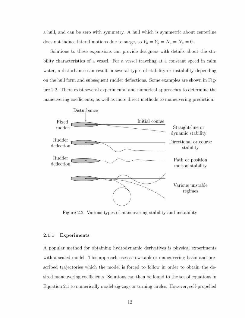
bility characteristics of a vessel. For a vessel traveling at a constant speed in calm
water, a disturbance can result in several types of stability or instability depending
on the hull form and subsequent rudder deflections. Some examples are shown in Fig-
ure 2.2. There exist several experimental and numerical approaches to determine the
maneuvering coefficients, as well as more direct methods to maneuvering prediction.
Initial course
Straight-line ordynamic stability
Path or positionmotion stability
Directional or coursestability
Disturbance
Fixedrudder
Rudderdeflection
Various unstableregimes
Rudderdeflection
Figure 2.2: Various types of maneuvering stability and instability
2.1.1 Experiments
A popular method for obtaining hydrodynamic derivatives is physical experiments
with a scaled model. This approach uses a tow-tank or maneuvering basin and pre-
scribed trajectories which the model is forced to follow in order to obtain the de-
sired maneuvering coefficients. Solutions can then be found to the set of equations in
Equation 2.1 to numerically model zig-zags or turning circles. However, self-propelled
12
model tests can also be performed which allow for direct prediction of the turning
circles and zig-zag maneuvers that are performed at full scale.
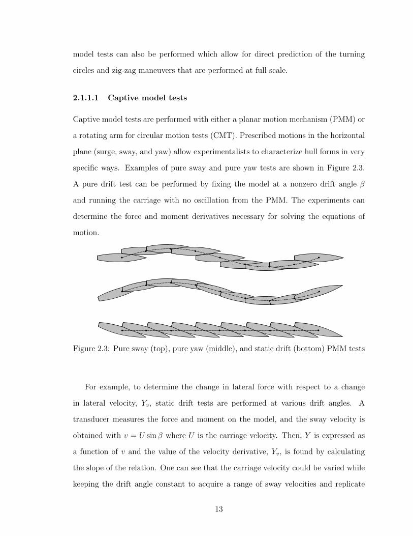
2.1.1.1 Captive model tests
Captive model tests are performed with either a planar motion mechanism (PMM) or
a rotating arm for circular motion tests (CMT). Prescribed motions in the horizontal
plane (surge, sway, and yaw) allow experimentalists to characterize hull forms in very
specific ways. Examples of pure sway and pure yaw tests are shown in Figure 2.3.
A pure drift test can be performed by fixing the model at a nonzero drift angle β
and running the carriage with no oscillation from the PMM. The experiments can
determine the force and moment derivatives necessary for solving the equations of
motion.
Figure 2.3: Pure sway (top), pure yaw (middle), and static drift (bottom) PMM tests
For example, to determine the change in lateral force with respect to a change
in lateral velocity, Yv, static drift tests are performed at various drift angles. A
transducer measures the force and moment on the model, and the sway velocity is
obtained with v = U sin β where U is the carriage velocity. Then, Y is expressed as
a function of v and the value of the velocity derivative, Yv, is found by calculating
the slope of the relation. One can see that the carriage velocity could be varied while
keeping the drift angle constant to acquire a range of sway velocities and replicate
13
the same experiment. However, Reynolds scaling can not be achieved due to the
unattainable speeds at which the carriage is required to move. Therefore, boundary
layers are not correctly scaled between the model and ship. This difference in viscous
effects is especially important near the transom when considering the forces on the
rudder – the most influential control surface in maneuvering.
The CMT method can also be used to find the derivatives for the equations of
motion. It works by moving the model in a circle about a vertical axis fixed in a
basin. The radius of rotation, drift angle, and yaw motion can be varied to obtain
the necessary derivatives. The PMM and rotating arm methods can also be per-
formed with rudders at various deflection angles and propellers operating at the ship
propulsion point. Therefore, both are suitable in providing information that can be
used to quantify nonlinear and cross coupling effects. Cross coupling is the effect that
force derivatives have on each other.
2.1.1.2 Free model tests
Compared to captive model tests, free model tests are a more direct approach at
predicting full scale maneuvering capabilities. Turning circles, zig-zags, and reverse
spirals can be performed using a remotely operated, self-propelled model. Several
criteria must be met for these tests to scale accurately. The propeller slip ratio of the
model and full scales should be equal. To satisfy this requirement, an air propeller
can be used to provide a portion of the thrust (Ueno et al., 2014). Also, the motor
powering the model propeller should be equipped with a thrust and torque transducer
to simulate the full scale engine characteristics that change during various maneuvers
(Pivano, 2008). This is sometimes ignored, resulting in model tests that predict less
speed loss than full scale tests. The inability to satisfy Reynolds scaling produces
inconsistencies between model and full scale boundary layer thicknesses. Propellers
have even been seen operating in a laminar regime (Cope, 2012). Turbulence inducing
14

measures can be implemented, but this scaling issue significantly restricts free model
tests from accurately predicting stopping maneuvers (ITTC, 2002). Overall, the
viscous force inaccuracies are even greater in free model tests than captive tests
because of the interactions between the rudder, propeller, and hull. In addition to
these difficulties, free model tests require large maneuvering basins to insure that
data are not affected by the tank boundaries and simply that there is ample space
in which to perform a full maneuver with a large model. Some facilities do not have
this capability. Thus, they are forced to perform partial maneuvers and extrapolate
data.
2.1.1.3 Systems based methods
Nonlinear maneuvering simulations in the time-domain can be performed with sys-
tems based methods. These mathematical models use force and moment derivatives
to solve the equations of motion. The derivatives can be obtained using empirical
data (Furukawa et al., 2008), model tests (Kim and Kim, 2008), or CFD (Simonsen
et al., 2012). The use of empirical data introduces uncertainty with the design of
original hull forms. Model tests and CFD are time-consuming, so while a maneu-
vering simulation may be fast with a systems based method, the data necessary to
solve the equations of motion are not easily gathered quickly. In addition, a lack of
consistency between models can be seen, showing a significant amount of sensitivity
due to different model inputs.
2.1.2 Numerical Simulations
Several state-of-the-art numerical approaches currently exist for examining the flow
around vessels undergoing steady or unsteady maneuvers. Ranging from inviscid
potential flow tools to fully nonlinear CFD, these methods vary widely in the resources
required and data attainable.
15
2.1.2.1 Inviscid methods
Potential flow methods for maneuvering prediction may be efficient due to the boundary-
integral nature of the formulation, opposed to solving equations in a field. And this
efficiency may appeal to designers. However, these approaches are also inviscid in
nature. Therefore, viscous separation is not resolved. Free surface elevations at large
drift angles and fluid forces on rudders are areas where the inviscid assumption sig-
nificantly affects predictions. For example, aft of the transom, rudders are positioned
in an area of highly rotational flow. The irrotational qualities stemming from the in-
viscid assumption make for poor predictions of the forces on rudders (Soding, 1999).
These forces are very important for maneuvering. Viscous approximations can be
made using empirical data or corrections from supplemental CFD simulations. Re-
sults from Kring et al. (2011) show good prediction of maneuvering forces on a surface
effect ship in waves using a potential flow method and viscous correction from CFD.
However, empirical data are limited to similar hull forms and may not be applicable to
novel designs. The use of CFD corrections can lead to questions of whether potential
methods possess enough fidelity for a wide range maneuvering prediction despite the
possibility of fully nonlinear, time-domain solutions (Tanizawa and Naito, 1998). The
overwhelming drawback lies in viscosity being neglected and challenges encountered
in trying to overcome this shortcoming.
2.1.2.2 Viscous methods
Common viscous methods solve for flow information on boundaries as well as within
fluid domains by seeking solutions to the URANS equations. Large-eddy simulation
(LES) is another viscous approach, but the URANS method is the main concern for
this nonlinear CFD discussion. The multiphase volume-of-fluid (VOF) method solves
the URANS equations in two fluids - air and water. Sufficient accuracy and numerical
stability depend on the adequacy of the grid refinement required to capture the air-
16
water interface. The computational cells (control volumes) need to be small in order
to resolve breaking waves, far-field waves, et cetera. Small time steps stem from these
highly resolved grids which are necessary even far from the hull. Work of Maki and
Wilson (2008) shows forces from a steady drift test using a VOF method that are very
comparable to experiments. Several free-running simulations on a variety of hulls are
shown in Shen et al. (2014).
A level-set approach can be used in a single phase or multiphase manner for
maneuvering prediction. Here, a signed distance function (level-set) is solved to de-
termine the location of the interface. Steep waves can be handled with this approach.
Simulations of captive model tests have been performed with a single phase level-set
to obtain maneuvering coefficients (Araki et al., 2014). In addition, free model turn-
ing circle and zig-zag tests have been simulated at model and full scale (Carrica et al.,
2012; Broglia et al., 2013).
Alternatives to surface capturing methods are surface tracking methods. These
use grid deformation to estimate an evolving free surface. Relatively simple forward-
speed resistance problems have been possible for some time (Kim, 2002). Surface
tracking has also been used for a numerical study on a constant turn maneuver (Burg
and Marcum, 2003). Small time-steps and numerical stability become issues since the
extent of grid deformations must be regulated. Surface tracking methods have issues
in the simulation of breaking waves due to the overturning of the wave and domain.
Finally, zero Froude number (double body) approximations enforce a flat free
surface. Therefore, the significant presence of the viscous effects is captured while
neglecting waves. Depending on the Froude number, this reduction in accuracy may
be accepted due to the increase in efficiency compared to multiphase approaches.
For example, maneuvering in ports or ship-to-ship operations are cases where this
method can yield accurate results. Turnock et al. (2008) suggests that double-body
simulations can be roughly 1,000% faster than a VOF approach. Low Froude number
17
simulations have been shown to compare well with experimental results of static drift
tests (Wang et al., 2008) and of pure sway tests (Turnock et al., 2008). Toxopeus
(2009) shows good agreement of bare hull forces to experiments when using double
approximations with Froude numbers less than Fr = 0.2. In addition, Broglia et al.
(2008) and Hochbaum et al. (2008) have performed pure yaw simulations with a flat
free surface.
Overall, nonlinear CFD can produce impressively accurate solutions of maneuver-
ing simulations. The VOF and level-set methods are two high-fidelity, well-studied
tools that should be utilized when the expense required for them is acceptable. The
capability of modeling the viscous effects in addition to a nonlinear free surface, pos-
sibly with breaking waves, is established as state-of-the-art. But these methods do
not greatly impact design because of expense, difficulty, and time.
2.1.3 Summary
Model tests require large facilities and the construction of accurately scaled models.
For low frequency PMM tests, even long tanks may allow for only two or three periods
of motion. The inability to satisfy Reynolds scaling severely affects the accuracy of
rudder-induced motions, especially with free model tests because the interactions
between hull, propeller, and rudder are not easily scaled. Furthermore, the need to
produce physical models is expensive and time-consuming which limits the amount
of changes one can make on a hull form. The cost of materials for a single 4.9 meter
model with propellers and rudders can be approximately 70,000 USD (Cope, 2012)
This is not conducive to hull form iterations required at early stages of design. The
limitations model tests and systems based methods pose for early phase design have
motivated the development of numerical methods.
Numerical methods possess their own set of limitations. Double-body formu-
lations give little information on the shape of the free surface and force an incor-
18
rect no-penetration condition on velocity. In turn, this adversely affects the solution
to the pressure in the flow which becomes problematic at Froude numbers greater
than Fr = 0.1. The use of surface tracking requires grid deformation which is time-
consuming and difficult to perform accurately, especially when breaking waves are
present. Likewise, the main drawback for each of the fully nonlinear methods is com-
putational expense. Even with recent advancements in parallel computing, the grid
refinement and computational requirements are burdening in nature. Currently, the
time and computational resources needed for these approaches make their use imprac-
tical in early stages of design. The need to include water and air portions within a
domain and the high grid resolution required, even far from the body, greatly increases
the number of cells.
The linearized URANS method aims to improve the maneuvering prediction capa-
bilities - from forward speed resistance tests to the simulation of free running model
tests - available to designers. The development of the technology embodies fast-
running simulations and simplified physics to more completely explore design spaces
for optimized solutions to modern naval architecture needs.
19

CHAPTER III
Free-Surface Boundary Conditions
The linearized URANS method is a single-phase approach to solving multiphase prob-
lems. Efficiency is sought through the use of a linearized free-surface approximation.
This is opposed to solving for an air-water interface or a nonlinear free-surface and re-
quires an investigation of the kinematic and dynamic boundary conditions associated
with a free-surface as well as an appropriate procedure for linearization. A discussion
of such matters is presented in this section.
3.1 The Air-Water Interface
In a physical setting, floating bodies pierce an air-water interface at which stresses
between the the two fluids are in balance. Therefore, the jump in stress is zero,[[σ · n
]]= 0. For more detail, see Rood (1995), van Brummelen (2002), and Yeh
(1995). An all-inclusive description of these stresses contains effects from surface ten-
sion. However, this cohesive molecular property is ignored in the present investigation
of ship flows. Bubbles, droplets, and other features that depend on surface tension
are not considered significant for maneuvering prediction compared to inertial and
viscous forces. As such, the stress (and force) from the water must be in balance with
20
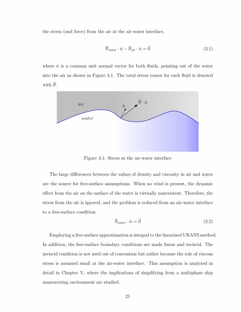
the stress (and force) from the air at the air-water interface,
σwater · n− σair · n = ~0 (3.1)
where n is a common unit normal vector for both fluids, pointing out of the water
into the air as shown in Figure 3.1. The total stress tensor for each fluid is denoted
with σ.
σ · nnair
water
Figure 3.1: Stress at the air-water interface
The large differences between the values of density and viscosity in air and water
are the source for free-surface assumptions. When no wind is present, the dynamic
effect from the air on the surface of the water is virtually nonexistent. Therefore, the
stress from the air is ignored, and the problem is reduced from an air-water interface
to a free-surface condition:
σwater · n = ~0 (3.2)
Employing a free-surface approximation is integral to the linearized URANS method.
In addition, the free-surface boundary conditions are made linear and inviscid. The
inviscid condition is not used out of convention but rather because the role of viscous
stress is assumed small at the air-water interface. This assumption is analyzed in
detail in Chapter V, where the implications of simplifying from a multiphase ship
maneuvering environment are studied.
21

3.2 Nonlinear Free-Surface Boundary Conditions
z, w
x, u
η (x, y, t) y, vn
Figure 3.2: Example of nonlinear free-surface
To develop linear kinematic and dynamic free-surface boundary conditions to com-
plement the viscous URANS equations, one must first consider the fully nonlinear
forms. Referring to Figure 3.2, the origin is located at the calm-water plane. Space
is represented in a three-dimensional, Cartesian manner with x, y, and z. The fluid
velocity vector, ~U = ui + vj + wk, contains components which act along the three
spatial axes. The free-surface elevation is η and is a function of x, y, and time, t.
Lastly, the unit vector, n, which is normal to free-surface everywhere and at all times,
points out of the water. The kinematic boundary condition requires that a particle on
the free-surface remains on the free-surface. This is shown with the relative velocity
between the fluid and the free-surface itself:
~U · n− ~Ufs · n = 0 (3.3)
~Ufs is the velocity of the free-surface. To express the condition in terms of the free-
surface elevation, the location of the free-surface may be defined with a function:
F (x, y, z, t) = z − η(x, y, t) = 0 (3.4)
The value of the function in 3.4 is always zero on the surface. As such, the total
22

derivative of the function is also zero on the surface:
DF
Dt=∂F
∂t+ ~U · ∇F = 0 (3.5)
Evaluating the total derivative of the free-surface function in terms of η results in:
−ηt + u (−ηx) + v (−ηy) + w = 0 (3.6)
By rearranging, the fully nonlinear kinematic free-surface boundary condition is ob-
tained:
w = ηt + uηx + vηy (3.7)
The dynamic free-surface boundary condition can be derived by invoking a zero
total stress condition. Since this is a free-surface, only the stresses in the water are
of concern, and the fluid subscript is dropped (σ = σwater). Deeming surface tension
insignificant for ship waves, the total stress tensor is composed of an isotropic term
and a viscous term:
σ = −PI + τ (3.8)
Here, P is the total pressure, I is the diagonal identity matrix, and the viscous stress
tensor is τ . The total pressure is composed of a hydrodynamic and a hydrostatic
part:
P = p+ ρ~g · ~x (3.9)
The gravitational acceleration vector is ~g, and the position vector is ~x. In conjunction
with the coordinate system currently in use, the hydrostatic pressure can be described
23

as follows:
~g = −gk (3.10)
ρ~g · ~x = −ρgz (3.11)
At the water surface, z = η. The incompressible viscous stress tensor is:
τ = µ
(∇~U +
(∇~U
)T)(3.12)
The dynamic viscosity is represented by µ. Expanding the viscous stress tensor gives:
τ = µ
(ux + ux
) (uy + vx
) (uz + wx
)(vx + uy
) (vy + vy
) (vz + wy
)(wx + uz
) (wy + vz
) (wz + wz
) (3.13)
Seeking a zero total stress boundary condition implies:
σ · n = ~0 (3.14)
The unit normal vector can be written as:
n = qi+ rj + sk (3.15)
In expanded form, the total stress vector appears as:
σ · n =
−(p− ρgz
)q + µ
(2uxq +
(uy + vx
)r +
(uz + wx
)s)
−(p− ρgz
)r + µ
((vx + uy
)q + 2vyr +
(vz + wy
)s)
−(p− ρgz
)s + µ
((wx + uz
)q +
(wy + vz
)r + 2wzs
) (3.16)
The function F = (x, y, z, t) from Equation 3.4 is used to express the normal vector
24

in terms of the free-surface elevation:
n =∇F| ∇F |
=−ηxi− ηy j + k√
η2x + η2
y + 1(3.17)
Using the normal vector from Equation 3.17 and performing the operation to ob-
tain the total stress vector, σ · n, results in the fully nonlinear, dynamic free-surface
boundary conditions in the x, y, and z-directions, respectively:
(p− ρgη) ηx − 2µuxηx − µ (uy + vx) ηy + µ (uz + wx) = 0
(p− ρgη) ηy − µ (vx + uy) ηx − 2µvyηy + µ (vz + wy) = 0
− (p− ρgη)− µ (wx + uz) ηx − µ (wy + vz) ηy + 2µwz = 0
(3.18)
This set of dynamic boundary conditions is nonlinear and coupled by the unknowns
of u, v, w, p, and η. They are to be satisfied on the z = η surface.
Lastly, the body boundary condition for the fully nonlinear problem states that
the velocity of the fluid is equal to the velocity of the body.
~U = ~Ubody (3.19)
The boundary conditions for the fully nonlinear ship maneuvering problem have
been presented. A free-surface assumption is made initially, and the implications of
this are shown in Chapter V with a viscous-interface study.
3.3 Linearized Free-Surface Boundary Conditions
With the goal of linearization, the free-surface boundary conditions need to be ex-
pressed in a form which is able to be satisfied on the z = 0 plane. This problem is
studied extensively within a velocity potential framework. Ship waves generated in
calm water described with the velocity potential variable by Kelvin (1887) lay the
25
foundation for decades of additional work. Continuous functions describe ship waves
for large domains as discussed in Noblesse et al. (2013, 2011). These show robust-
ness and efficiency of applying a linearized free-surface approximation. Additional
work extends to ship motions in the presence of incident waves (Beck and Loken,
1989; Salvesen et al., 1970) as well as waves described in an inertial reference frame
(Noblesse and Yang, 2007). Comparisons of a linear approximation as apposed to
a nonlinear free-surface are also considered with velocity potential (Havelock, 1937,
1940). This inviscid approach is shown to provide solutions to very complex problems
such as dredging in a shallow water channel in Beck et al. (1975). Overall, the lin-
earized free-surface boundary conditions alone are not new. However, exploring the
suitability of a linearized free-surface in conjunction with a viscous, turbulent fluid is
a unique endeavor; one that is important for the viscous, unsteady problem of ship
maneuvering.
For this work, it is assumed that the waves associated with ship maneuvering
are predominantly of small height and small slope. Thus, a first-order wave approx-
imation will suffice while ignoring nonlinear and breaking waves. To display this
mathematically, the free-surface conditions must first be made dimensionless to eval-
uate the relative values of each term. Quantitatively, the small slope assumption
implies that | ηx |, | ηy |� 1. What follows is a process for linearization which one
may pursue stemming from this assumption, as well as further inviscid assumptions
within the dynamic condition resulting in wave effects that are solvable on the z = 0
plane.
Beginning again with the fully nonlinear kinematic free-surface boundary condi-
tion shown in Equation 3.7, one can consider a fluid moving past a floating body.
From the perspective of a body-fixed observer, the horizontal components of the fluid
26
velocity vector can be decomposed into a mean and perturbing component:
u = U + u∗
v = V + v∗
w = W + w∗
(3.20)
The mean components are represented with U , V , and W , while the perturbation
velocities are denoted with u∗, v∗, and w∗. For a forward speed ship resistance test,
the mean velocity may simply be the mean surge velocity with respect to time, but
a mean velocity is more difficult to define for a transient maneuver. Using decom-
posed velocities from Equation 3.20 in the fully nonlinear kinematic condition from
Equation 3.7 results in the following modified nonlinear kinematic condition:
W + w∗ = ηt + (U + u∗) ηx + (V + v∗) ηy (3.21)
In order to determine the relative magnitude of each term in Equation 3.21, each
quantity is represented non-dimensionally with U , L, and T . U is some suitable
velocity scale, possibly the ship speed; L is the ship length or possibly a wave length;
27
and T is a time scale, perhaps a wave period. Each quantity is made dimensionless:
W =W
Uw∗ =
w∗
Ut =
t
T
U =U
U= 1 u∗ =
u∗
Uη =
η
L
V =V
Uv∗ =
v∗
Ux =
x
L
ηx =L
Lηx = ηx ηy = ηy y =
y
L
ηt =T
Lηt
(3.22)
Assuming perturbation velocities, wave slopes, and wave heights are on the order of
some small value, O (ε), an order-or-magnitude analysis is performed. Substituting
the values from Equation 3.22 into the fully nonlinear condition of Equation 3.21 and
dividing by U gives the dimensionless equation:
W +w∗ =L
UTηt +U ηx +u∗ηx +V ηy +v∗ηy
O (ε) = O (ε) +O (ε) +O (ε2) +O (ε) +O (ε2)(3.23)
Only horizontal motions are performed with the linearized URANS method. As such,
there is no mean vertical velocity, W = 0. Furthermore, higher order terms, O (ε2),
are very small and neglected resulting in the linear kinematic free-surface boundary
condition, shown dimensionally:
w = ηt + Uηx + V ηy (3.24)
The magnitude of the mean velocities depends on the frame of reference in which
the maneuvering problem is described. For a forward speed resistance problem rep-
28

resented in a ship-fixed reference frame, U = Uship and V = Vship = 0. Thus, the
kinematic free-surface boundary condition in this ship-fixed description is reduced to
a linearized form:
w = ηt + Uηx (3.25)
In an earth-fixed frame of reference, calm water has a zero mean velocity, U = V = 0.
Only perturbation velocities exist as the hull disturbs the calm water. Again, these
are deemed small, and the linear kinematic free-surface boundary condition in an
Earth-fixed frame of reference is obtained. It is known as the zero-speed kinematic
condition:
w = ηt (3.26)
A slightly different approach needs to be taken for the dynamic free-surface bound-
ary conditions in Equation 3.18. The wave slope and wave height are considered small,
but less can be said about the velocity gradients on the surface of the water. As a
starting point, one can again select velocity and length scales with which to charac-
terize the problem. Commonly with ship flows, the ship speed and ship length are
chosen for these scales. As such, the non-dimensional Reynolds and Froude numbers
are used, respectively,
Re =UL
ν=ULρ
µ(3.27)
Fr =U√gL
(3.28)
where U is the speed of the ship, L is the length of the ship, ν is the kinematic
viscosity, ρ is the water density, and g is the magnitude of gravity. In addition to
the use of Reynolds and Froude numbers for viscous and gravitational terms, each
29

remaining term in Equation 3.18 can be represented non-dimensionally:
p =p
12ρU2
η =η
L
∇~U ij =∇~Uij
U/L
The ship speed and length are suitable quantities for non-dimensionalizing the gravity
waves which govern the hull forces. After all, the fundamental wavelength, λ, of ship
generated waves in deep water is defined using these quantities:
λ
L=
2πU2
gL(3.29)
However, these scales are not representative of the boundary layer flow near the hull.
To some extent, this boundary layer interacts with the water surface, so caution must
be used when using the ship length, L, as the length scale for dimensionless analysis
with this viscous problem. Applying this non-dimensional analysis to the nonlinear
dynamic conditions, and dividing by 12ρU2, offers insight into the possible significance
of each term with following the dimensionless equations:
(p− 2Fr−2η) ηx − 4Re−1uxηx − 2Re−1 (uy + vx) ηy + 2Re−1 (uz + wx) = 0
(p− 2Fr−2η) ηy − 2Re−1 (vx + uy) ηx − 4Re−1vyηy + 2Re−1 (vz + wy) = 0
− (p− 2Fr−2η)− 2Re−1 (wx + uz) ηx − 2Re−1 (wy + vz) ηy + 4Re−1wz = 0
(3.30)
Again, the boundary layer presents ambiguity in determining the relative magnitudes
of each quantity in Equation 3.30 because the velocity gradients may be large, and
the length and velocity scales differ significantly from those used to describe the ship
generated waves. If one assumes small velocity gradients in addition to the small wave
slopes, the products of the two are negligible or O (ε2). This assumption produces
30
dynamic conditions which are linear:
2Re−1 (uz + wx) = 0
2Re−1 (vz + wy) = 0
− (p− 2Fr−2η) + 4Re−1wz = 0
(3.31)
Furthermore, Reynolds numbers are generally large for ship flows, resulting in
small viscous terms in Equation 3.31. Neglecting all viscous terms in the dynamic
condition results in a single, zero total pressure condition.
p− 2Fr−2η = 0 (3.32)
However, the assumption of large Reynolds number raises questions. Indeed, typical
Reynolds numbers are at least O (105) for model scale. But these scales may not be
an appropriate description for maneuvering flows. Certainly, the turbulent flow in
the wake region aft of the transom contains length and velocity scales that are much
shorter and slower than outside of the wake. Therefore, smaller lengths scales may
be a more suitable representation of the flow in this region.
A variety of work has been conducted using different forms of the dynamic bound-
ary conditions. Studies by Shen et al. (1999, 2000, 2002) implement the viscous lin-
earized boundary conditions (Equation 3.31) for investigating the flow in the wake
of a towed ship model. The model Reynolds and Froude numbers are O (103) and
O (10−2), respectively, and the beam is only four centimeters (Shen et al., 2002). It
is found that the x and y components of the dynamic condition are very small at the
water surface, but also that the wakes of real ships contain significantly more tur-
bulence. Work by Rosemurgy et al. (2012) shows good results for free-surface flows
using the inviscid, zero total pressure condition (Equation 3.32). Reynolds numbers
for this work are O (105), but submerged bodies are studied in a steady manner. In
31

addition, Hong and Walker (2000) investigate free-surface flows with submerged jets.
The jet diameter Reynolds number is O (104), and the Froude number is O (101).
Viscosity is deemed negligible due to the high Reynolds number, but the absence of
no-slip boundary conditions also influences this assumption.
The various problems, approaches, and conclusions in previous work prompts the
need for a unique set of studies to determine the effect of viscosity and vorticity at the
air-water interface of maneuvering flows. The goal of the present work is to extend the
investigation of free-surface flows to large Reynolds and Froude numbers. In order to
perform a thorough investigation, the entire fully nonlinear dynamic conditions from
Equation 3.30 are studied. No a priori assumptions are made about the wave slopes,
the velocity gradients, or eddy viscosity. This allows for a quantitative examination
of the importance of each term in the zero total stress condition. The geometry
used for this problem is that of a two-dimensional ship transom and is presented in
Chapter V.
32
CHAPTER IV
Linearized Free-Surface Solver
4.1 ALE Formulation
The equations that govern the free-surface elevation are linearized, i.e. first-order
kinematic and dynamic boundary conditions that are solved on the z = 0 plane.
w =∂η
∂t(4.1)
p− ρgη = 0 (4.2)
Due to the linearization, the computational domain where the momentum equations
are solved does not extend above the z = 0 calm-water plane. Body exact ship
motions are limited to surge, sway, and yaw. These horizontal-plane motions are
performed in an inertial, Earth-fixed reference frame that necessitates an arbitrary
Lagrangian-Eulerian (ALE) formulation of the governing equations. Equations are
solved for each computational cell that has volume V and is bounded by the surface
S with outward normal n. So (t) is the portion of the boundary of a computational
cell that is adjacent to the z = 0 plane, and l (t) is the contour of this area. The
development of the ALE form of the kinematic free-surface boundary condition begins
33

with the Leibniz integral rule applied over a surface to the right-hand side of Eq. 4.1,
∂
∂t
∫So(t)
η dS =
∫So(t)
∂η
∂tdS +
∫l(t)
η∂~xmesh (t)
∂t· n dl (4.3)
where,
∂~xmesh (t)
∂t= ~Umesh = umeshi+ vmeshj + 0k (4.4)
Equation 4.3 can be modified to appear as:
∫So(t)
∂η
∂tdS =
∂
∂t
∫So(t)
η dS −∫l(t)
η~Umesh · n dl (4.5)
With this, one can see that the mesh motion gives rise to a convective term in the
ALE formulation of the kinematic free-surface boundary condition. And the form of
the condition solved is:
∂
∂t
∫So(t)
η dS −∫l(t)
η~Umesh · n dl =
∫So(t)
w dS (4.6)
Similarly, the ALE form of the momentum and continuity equations is solved,
∂
∂t
∫V
ρ~U dV +
∫S
ρ~U ~Urel · n dS = −∫S
p · n dS +
∫S
µeff
(∇~U +∇~UT
)· n dS (4.7)
∫S
~Urel · n dS = 0 (4.8)
where,
~Urel = ~U − ~Umesh (4.9)
and the effective viscosity is the sum of the molecular and turbulent viscosities,
µeff = µ + µt.
34

4.2 Boundary Condition at Free-Surface/Body Juncture
In physical settings and nonlinear simulations of ship maneuvering, the height of the
water level varies along the hull. If using a VOF method, a macroscopic boundary
condition for the phase indicator variable, α, on the hull is a Neumann condition
where the gradient of α is zero in the direction of the normal vector on the body:
∇α · n = 0 (4.10)
The zero-gradient condition allows bow waves to force water above the calm waterline
and ventilated transom sterns to lower the surface to the depth of the transom. These
phenomena raise challenges for the linearized free-surface method, especially near the
transom. Since the free-surface elevation is calculated on a rigid z = 0 plane, the
domain level around the hull never actually changes. Therefore, a unique boundary
condition is required for the free-surface elevation on the body. Transom sterns that
become ventilated during an unsteady simulation pose the greatest risk for divergence
with the linearized URANS method. A zero-gradient condition is suitable on the
majority of the hull, but a Dirichlet condition is useful in the transom region. A
Dirichlet condition specifies the value of the free-surface elevation. As such, users may
set the free-surface elevation to the depth of a ventilated transom. The capability to
impose both Neumann and Dirichlet conditions on the hull is possible with the use
of a Robin or mixed condition, in discretized form:
η = Vf (ηbc) + (1− Vf ) ηp (4.11)
Vf is the volume-fraction that dictates the blending of a fixed-value and zero-
gradient in the condition. The volume-fraction can take values from 0 ≤ Vf ≤ 1. A
value of Vf = 1 makes the free-surface elevation on the body equal to a user-specified
35

fixed-value, ηbc. A value of Vf = 0 activates a zero-gradient (Neumann) condition
which makes the free-surface elevation equal to the value at the center of the cell
adjacent to the boundary, ηp. The value of Vf is computed with Equation 4.12:
Vf = Cm
[max
(0,
1
1− Ct
(−nf ·
~Uship
| ~Uship |− Ct
))](4.12)
Here, Uship is the velocity of the body, and nf is the outward pointing normal of the
body. The transition coefficient, Ct, is a user-specified value ranging from 0 ≤ Ct < 1
that helps determine the location where the boundary condition will transition from
Neumann to Dirichlet. If the angle between the velocity vector of the body and the
outward-pointing normal of the body is less than arccos (Ct), Vf will be set to zero,
and the boundary condition will be fully zero-gradient (Neumann). However, if the
angle between the velocity and outward-pointing normal is greater than arccos (Ct),
the condition is partially fixed-value and zero-gradient. When the flow is aligned
with the normal, Vf = 1, the condition becomes fully fixed-value (Dirichlet). Cm is a
multiplication coefficient a user can change to further modify the boundary condition.
This approach for the boundary condition for η at the free-surface/body juncture is
very useful. A user can calculate the transom-based Froude number to determine if
a transom stern is ventilated. Then the geometry of the hull can be considered along
with the type of maneuvering test to set an angle with Ct at which the free-surface
elevation will be fixed at a certain value (perhaps the depth of the transom).
As an example, a hull with an elliptic water-plane cross-section is considered. It
translates purely in the (+x)-direction with some velocity, ushipi. Figure 4.1 shows
the region on the hull where the boundary condition is mixed for several values of
Ct. For this example, the free-surface elevation forward of midship is always governed
by the Neumann, zero-gradient condition, where Vf = 0. Depending on the value of
Ct, the condition becomes mixed at some point aft of midship. All instances of the
36

condition become Dirichlet-type at the stern where the outward pointing normal is
aligned with the ship velocity.
0
0.25
0.5
0.75
1
-0.5 -0.25 0 0.25 0.5
Vf
Cm
x
Lpp
Ct = 0.01Ct = 0.1Ct = 0.2Ct = 0.3
Figure 4.1: Free-surface body boundary condition with varying Ct values
4.3 Numerical Aspects
The linearized URANS method is a custom finite volume CFD algorithm based within
the OpenFOAM C++ library. It consists of solutions to the URANS equations and
a linear free-surface condition. At the free-surface, values for the wave elevation, η,
are solved at cell centers and interpolated onto cell faces.
Results discussed in this paper are obtained on structured and unstructured grids.
A PISO-like algorithm is used to solve for pressure and velocity. Time discretization
is performed with a first-order Euler implicit scheme. A second-order linear upwind
scheme is used for convective terms. The Spalart-Allmaras turbulence model is used
with an adaptive wall function based on the Spalding universal law of the wall.
To simulate motions in the horizontal plane, the entire computational domain
moves with rigid-body motion. The ship motion is described in an inertial, Earth-fixed
reference frame. This approach allows for a natural description of the acceleration
of the body from rest and avoids issues related to an impulsive start. Furthermore,
it closely resembles the actual motions in a physical setting (which in this validation
37

is a towing tank). While the entire grid undergoes rigid body motion, propellers
and rudders rotate relative to the body with a sliding-mesh approach. A cylinder
enclosing a propeller or rudder rotates independently from the remainder of the mesh.
Figure 4.2 describes the steps of the algorithm with the unique features outlined in
red. The solution of the momentum equations provides the vertical velocity which
is used in the kinematic boundary condition. In a typical segregated manner, the
pressure equation is then solved and used to correct the velocities at cell centers.
Upon updating the boundary conditions over the computational domain, the pressure
condition on the free-surface uses the wave elevation from the kinematic condition
to apply the hydrostatic pressure. Steady problems can be modeled by using time
steps to dictate the number of iterations with no inner correctors, outer correctors,
or time-derivatives. For unsteady problems, time steps can dynamically adjust to a
user-defined Courant number restriction. For stability, inner correctors can be used
to solve the momentum equations multiple times within a single time step. Lastly,
under-relaxation may be employed in combination with outer correctors for time-
accurate solutions employing large time steps.
38

Start
End
Inner
corr
ecto
rs
Outer correctors
Time steps
Set boundaryconditions
Solvemomentumequations
Computeflux on cell
faces
Solve forη
Correct~U
Correct fluxon cell faces
Solvepressureequation
Updateboundaryconditions
Applyp = ρgη on
f-s
Solve for∆t
Figure 4.2: Steps of the linearized URANS algorithm
4.4 KCS Validation
As an initial validation of the linearized free-surface boundary conditions, the KRISO
container ship (KCS) hull is studied at forward speed over a range of Froude num-
bers. Although the ultimate goal is maneuvering prediction, requiring the accurate
solutions to forces and moments, this relatively simple study provides an opportunity
to view the wave height along the hull as well as predictions of sinkage and trim.
Vertical motions are not performed with the linearized RANS method, but the heave
and pitch can be calculated with an approach consistent with linear theory using
39
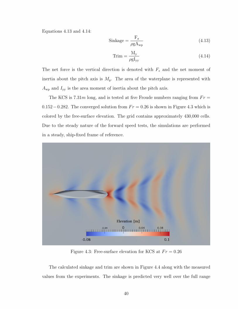
Equations 4.13 and 4.14:
Sinkage =Fz
ρgAwp
(4.13)
Trim =My
ρgIyy
(4.14)
The net force is the vertical direction is denoted with Fz and the net moment of
inertia about the pitch axis is My. The area of the waterplane is represented with
Awp and Iyy is the area moment of inertia about the pitch axis.
The KCS is 7.31m long, and is tested at five Froude numbers ranging from Fr =
0.152−0.282. The converged solution from Fr = 0.26 is shown in Figure 4.3 which is
colored by the free-surface elevation. The grid contains approximately 430,000 cells.
Due to the steady nature of the forward speed tests, the simulations are performed
in a steady, ship-fixed frame of reference.
Figure 4.3: Free-surface elevation for KCS at Fr = 0.26
The calculated sinkage and trim are shown in Figure 4.4 along with the measured
values from the experiments. The sinkage is predicted very well over the full range
40

of Froude numbers with the linearized RANS method. The largest discrepancy com-
pared to the experimental data is approximately one millimeter occurring at the high
and low Froude number limits. The trim angles agree well at the low Froude num-
bers, but show increasing differences at higher Froude numbers. However, the largest
difference between the simulations and experiments is still roughly 0.1 degrees.
0.000
0.005
0.010
0.015
0.020
Sin
kage
[m]
Lin. RANSExperimental
-0.3
-0.2
-0.1
0.0
0 0.05 0.1 0.15 0.2 0.25 0.3 0.35
Tri
m[◦
]
Fr [−]
Figure 4.4: Sinkage (top) and trim (bottom) of KCS at various Froude numbers.Values are measured for the experiments and computed for the simulations
The wave elevation along the hull is presented in Figure 4.5 for Froude number
Fr = 0.26. The linearized data agrees well along the majority of the hull. However,
there is a noticeable under-prediction near the bow and an over-prediction at the
stern. For this study, a zero normal-gradient condition is used for the free-surface
boundary condition at the free-surface/body juncture. In Section 4.2, a custom body
boundary condition is presented which aids in mitigating the discrepancies that are
possible to produce with a zero normal-gradient condition.
41

-0.010
-0.005
0.000
0.005
0.010
0.015
0 0.25 0.5 0.75 1
η Lp
p
[−]
x
Lpp
[−]
Lin. RANSExperimental
Figure 4.5: Wave along KCS hull at Fr = 0.26
42

CHAPTER V
Viscous Air-Water Interface Study
5.1 Canonical Viscous Interface Study
In order to quantify the relative importance of each term in the fully nonlinear dy-
namic free-surface boundary condition, a canonical study is performed with a two-
dimensional transom stern geometry. An interface capturing approach is employed
by using a fully nonlinear VOF method. This allows one to quantify the effects of
reducing problems from an air-water interface to a free-surface, as well as the effects
of linearization and the neglect of viscous terms. A diagram of the two-dimensional
ship transom is shown in Figure 5.1.
The two-dimensional transom study is a challenging problem for the linear method.
The entire domain is filled with water below the z = 0 calm-water plane. However,
wave elevations oscillate some small value, η, about the flat free-surface. So, the
linear approximation possesses an interesting feature - the conservation of mass and
momentum is satisfied for a single phase in each computational cell, but the pressure
within these cells can correspond to being filled with either water or air. For example,
in the case of a ventilated transom stern, a trough of the wave is located at the bottom
of the transom. The linearized method has computational cells above this trough,
but the dynamic pressure within them corresponds to the hydrostatic pressure at the
base.
43
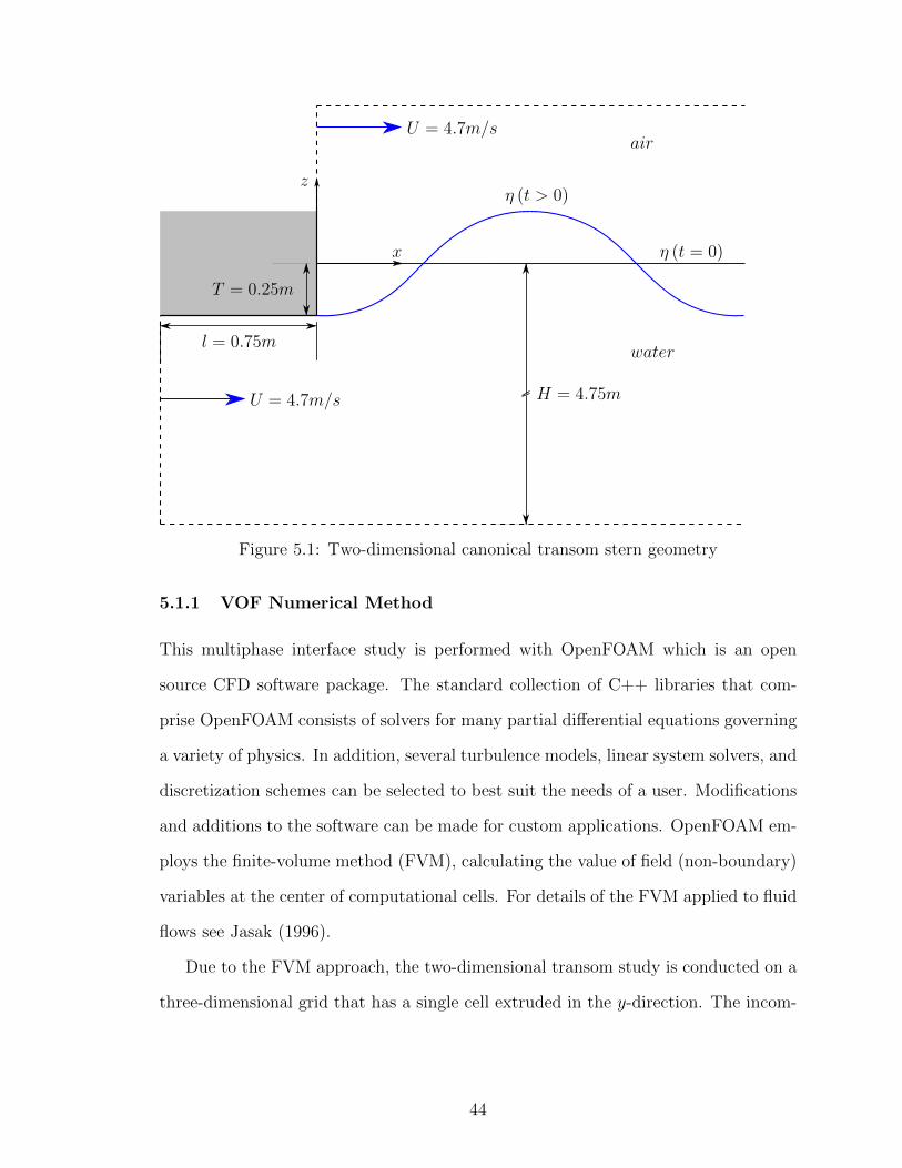
η (t > 0)
η (t = 0)
z
x
U = 4.7m/s
l = 0.75m
H = 4.75m
T = 0.25m
U = 4.7m/sair
water
Figure 5.1: Two-dimensional canonical transom stern geometry
5.1.1 VOF Numerical Method
This multiphase interface study is performed with OpenFOAM which is an open
source CFD software package. The standard collection of C++ libraries that com-
prise OpenFOAM consists of solvers for many partial differential equations governing
a variety of physics. In addition, several turbulence models, linear system solvers, and
discretization schemes can be selected to best suit the needs of a user. Modifications
and additions to the software can be made for custom applications. OpenFOAM em-
ploys the finite-volume method (FVM), calculating the value of field (non-boundary)
variables at the center of computational cells. For details of the FVM applied to fluid
flows see Jasak (1996).
Due to the FVM approach, the two-dimensional transom study is conducted on a
three-dimensional grid that has a single cell extruded in the y-direction. The incom-
44

pressible URANS equations are solved in both air and water:
∂ρ~U
∂t+∇ · ρ~U ~U = −∇p+∇ ·
[(µ+ µτ )
(∇~U +∇~UT
)](5.1)
∇ · ~U = 0 (5.2)
The dynamic eddy viscosity is represented with µτ and arises due to modeling the
fluctuating components after Reynolds-averaging. The solution to µτ is obtained
using the one-equation Spalart-Allmaras turbulence model (Spalart and Allmaras,
1992). The pressure-velocity coupling is handled in a segregated manner where these
variables are decoupled and solved implicitly. For a thorough description of this
approach see Barton (1998) and Issa (1986).
The air-water interface is captured using a VOF method. This technique is
well suited for large deformations between fluids with significant differences in den-
sity (Hirt and Nichols, 1981; Lafaurie et al., 1994). Two fluids are treated as one
continuous fluid composed of two regions with different properties of density and
viscosity:
ρ (~x, t) = ρwaterα (~x, t) + ρair (1− α (~x, t)) (5.3)
µ (~x, t) = µwaterα (~x, t) + µair (1− α (~x, t)) (5.4)
The locations of the air and water regions are determined by the value of the phase-
indicator variable, α, which varies from zero to one throughout the domain. Cells
occupied by water have a value of α = 1, and cells occupied by air have a value
of α = 0. The interface is not sharp but rather smeared across multiple cells. Those
cells at the interface have values of 0 < α < 1. The solution to the phase-indicator
variable is governed by an advection equation,
∂α
∂t+∇ ·
(α~U)
+∇ ·(α (1− α) ~UrCα
)= 0 (5.5)
45

where ~Ur is a compression velocity which acts normal to and towards the interface. It
helps regulate the smearing of the interface, and it is only active where 0 < α < 1. The
coefficient Cα allows a relative magnitude of the compression velocity to be applied.
For this study, the value of Cα is constant, Cα = 1
Time discretization is performed with a first-order implicit Euler scheme. Inte-
gration over faces is done with a second-order midpoint rule. Lastly, the divergence
operator is discretized with a second-order upwind-biased scheme for velocity and a
van Leer limited scheme for the phase indicator variable. The equation for the phase
indicator variable is solved in an explicit manner. The linear systems of equations
are solved with a generalized geometric-algebraic multi-grid (GAMG) solver.
5.1.2 Description of Canonical Problem
The purpose of these studies is to determine the dominant terms that govern the
pressure at the water surface of an air-water interface. In particular, the effects of
viscosity and velocity gradients are of interest in order to reach a clear conclusion of
which terms to include when choosing a pressure boundary condition for the linearized
URANS method. Due to the unsteady nature of maneuvering, a variety of flow is
produced. Breaking waves, non-breaking waves, large areas of recirculation, and rel-
atively calm water can all be witnessed. To account the for range of phenomena, nine
combinations of Reynolds numbers and transom-based Froude numbers are tested as
shown in Table 5.1. The transom-based Froude number is defined in Equation 5.6.
For each simulation, the initial values of the kinematic eddy viscosity, ντ , on the inlet
are equal to the molecular kinematic viscosities shown in Table 5.1.
Table 5.1: Two-dimensional transom test viscosity and gravity variable values
Re ν [m2/s] FrT g [m/s2]1e4 3.52e− 4 3 9.811e5 3.52e− 5 2 22.11e6 3.52e− 6 0.2 2207
46
FrT =U√gT
(5.6)
The work of Maki (2006) studies transom stern hydrodynamics and discusses the
highly unsteady nature of the flow at particular Froude numbers. This is useful
for choosing the transom-based Froude numbers for the numerical experiments at
hand. A Froude number of FrT = 3 produces a steady wave, FrT = 2 produces
an unsteady breaking wave, and FrT = 0.2 produces a recirculation region with a
nearly flat air-water interface. Therefore, these Froude numbers display flows which
commonly occur near ship hulls during maneuvering.
The main reason behind changing the values of gravity and viscosity is to use the
same grid for each test. Since velocity, U , is a shared variable between the Reynolds
and Froude numbers, changing it requires new grids with subsequent changes of
length, l, and draft, T . The current approach avoids this issue. However, chang-
ing the value of viscosity while not changing the grid spacing adjacent to the no-slip
boundary condition presents issues with the dimensionless wall distance, y+:
y+ ≡√
τwρν2
(5.7)
τw = µ
(∂u
∂z
)wall
(5.8)
The wall shear stress is denoted with τw and defined in Equation 5.8 using the coor-
dinate system for these experiments. With low-Reynolds number turbulence models,
the dimensionless wall distance is required to be y+ < 1. To overcome this restric-
tion, an adaptive wall function is used to account for the average y+ values for these
experiments which are within the range 0.1 < y+mean < 50. Table 5.2 shows the mean
and maximum y+ values for each simulation.
47

Table 5.2: Two-dimensional transom test y+ values
FrT = 3 FrT = 2 FrT = 0.2Re y+
mean y+max y+
mean y+max y+
mean y+max
1e4 1.49 2.46 1.87 4.16 0.71 2.311e5 5.41 8.38 5.13 9.28 3.29 7.491e6 30.13 97.39 33.27 105.42 18.21 41.48
The grid for the study is fully structured and consists of approximately 2.9M
entirely orthogonal cells. The resolution of the grid in the interface region is of great
importance due to the smearing of the interface over multiple cells with the VOF
method. To minimize the distance over which the smearing occurs, the back face
of the transom is discretized with 598 cells, each with a height of roughly 0.83mm.
Gradual stretching is employed from the bottom and back faces of the transom. A
qualitative representation of the grid appears in Figure 5.2.
z
x
∆x ∗ 89
∆z ∗ 46
Figure 5.2: Transom grid characteristics. Cell dimensions adjacent to the transomare scaled for visualization. The stretching away from the transom is not to scale andis only meant for a qualitative description.
48

5.2 Results
The results from the two-dimensional transom stern study are divided into three sec-
tions corresponding to the three Froude numbers tested. The goal of the experiments
is the same for all cases – to measure the suitability of the linearized free-surface
conditions for maneuvering prediction. As a starting point, it must be shown that
indeed an interface condition is satisfied. Therefore, the total stress of each fluid at
the air-water interface is a concern for this investigation:
σwater,air · n =[− (p− ρwater,airgη) I + τ
]· n
=
[− (p− ρwater,airgη) I + µeffwater,air
(∇~U +
(∇~U
)T)]· n
(5.9)
For each Froude number, the terms which make up the total stress tensor will be
considered in slightly different ways to best describe the important flow characteristics
at hand. The beginning of each section contains a brief description of the way in which
the terms will be evaluated. First, the cases with FrT = 3 are presented. This Froude
number produces a steady wave, so two-dimensional plots are used to convey results
which show the air-water interface condition and the small role of viscosity in the
free-surface condition. Next, the cases with FrT = 2 are presented. With these, an
unsteady breaking wave is generated, so iso-surfaces are used to show the small values
of viscous stress and the balance between hydrostatic and hydrodynamic pressure at
different moments in time. Lastly, cases where FrT = 0.2 are the low Froude number
regime, and two-dimensional plots are again used to analyze this steady set of data.
Within each Froude number, the tests appear in order of increasing Reynolds
number (Re = 1e4, 1e5, and 1e6). Turbulence modeling is performed with the
Spalart-Allmaras turbulence model, so viscous terms are shown using the effective
viscosity µeff = µ + µt. The study is two-dimensional, thus only the variables cor-
responding to the x and z-directions are reported. Also, all pressure and stress
49
quantities are presented in non-dimensional form, normalized by1
2ρwaterU
2, unless
otherwise noted. This is simply used as a stress scale that corresponds to the stagna-
tion pressure at the calm-water elevation, or the largest possible dynamic pressure in
the flow under the irrotational assumption. A tilde is used above terms to symbolize
dimensionless quantities. The downstream distance is non-dimensionalized by the
fundamental wave length, λ, which is calculated for each Froude number:
λ = 2πFr2TT (5.10)
The cases of FrT = 3 and FrT = 0.2 include a study of the kinematic condition
by plotting the nonlinear and linear forms, respectively:
w = uηx (5.11)
w = Uηx (5.12)
The vertical velocity at the surface of the water is w. The horizontal velocity from
the solution is u, and the linear constant velocity from the inlet is U = 4.7m/s. When
presented, these quantities from the kinematic condition are normalized by U .
Lastly, each section concludes with a comparison of the canonical study computed
with the linearized URANS method, and the suitability of transferring the boundary
conditions from the z = η to the z = 0 plane is discussed. The geometry and
magnitudes of gravity of the linear simulations are equivalent to those of the nonlinear
simulations. However, the mesh does not extend beyond the z = 0 plane, and it
contains only 7,909 computational cells.
50
5.2.1 FrT = 3 – Steady Wave
This section presents the results from the highest Froude number tested, FrT =
3. The wave length corresponding to this flow is λ ≈ 14.1m. As such, the water
depth corresponds to an intermediate-depth condition, but the boundary condition
employed on the bottom of the domain is not impenetrable. Instead, it is a zero
normal-gradient condition, ∂~U∂n
. Therefore, bottom effects are not as significant as
with a physical boundary at this depth. The stress balance interface condition is
shown to be satisfied, and the linearized free-surface condition is shown to be a
reasonable assumption for this flow. Due to the steady nature of the non-breaking
wave, the common normal vector is expressed in terms of the wave elevation:
n =−ηxi+ k√η2x + 1
(5.13)
First, the wave profiles are shown. Next, the stress in each fluid is considered to
ensure that the interface condition is satisfied:
σwater · n− σair · n = ~0 (5.14)
From here on, the air is no longer studied, but the suitability of the free-surface
approximation is investigated by considering stress terms from the water only:
σ · n =
(p− Fr−2η) ηx − 2Re−1uxηx +Re−1 (uz + wx)
− (p− Fr−2η) − Re−1 (wx + uz) ηx + 2Re−1wz
(5.15)
The horizontal and vertical components of the stress vector are discussed individu-
ally. The viscous terms from the rate-of-strain tensor are presented. For brevity, a
conservative approach is taken where the magnitude of each term is calculated, and
these are summed giving insight into the total effect that the viscous terms have on
51

the water surface:
| −2µeffuxηx | + | µeff (uz + wx) |0.5ρwaterU2
(5.16)
| −µeff (wx + uz) ηx | + | 2µeffwz |0.5ρwaterU2
(5.17)
Lastly, the hydrodynamic and hydrostatic pressure are compared. Only the terms
from the vertical component of the stress vector, p and ρgη, are plotted as these are
representative of the terms from the horizontal component, pηx and ρgηηx, which are
simply scaled by the wave slope.
-1.2
-0.8
-0.4
0.0
0.4
0.8
1.2
0 0.5 1 1.5 2
η T[−
]
x
λ[−]
Re=1e4Re=1e5Re=1e6
Figure 5.3: Wave elevations
The wave height for all the tested Reynolds numbers is shown in Figure 5.3. This
is a steady wave that develops and remains for the duration of the simulation. One
can see that the transom, with a depth of T = 0.25m, is fully ventilated under these
conditions. The difference in Reynolds number results in no significant variation in
the wave height.
The boundary layer profiles corresponding to each Reynolds number are presented
in Figure 5.4. These are sampled one transom depth, T , forward from the transom
edge. As expected, an increase in Reynolds number shows a thinning of the boundary
layer thickness.
To investigate the accuracy with which the interface condition is satisfied, the
52
-1.4
-1.2
-1.0
0 0.5 1
z T[−
]
u
U[−]
Re=1e4Re=1e5Re=1e6
Figure 5.4: Boundary layer velocity profiles
modulus of the total stress vector dotted with the common unit normal, | σ · n |,
is calculated for air and water. These magnitudes are plotted in Figure 5.5. To
differentiate the two fluids, a contour of α = 0.99 is used for water and α = 0.01 for
air. As such, the finite region that contains the interface is largely ignored. These
phase-indicator variable restrictions are chosen as a conservative approach to identify
stresses which very nearly correspond to either air or water rather than the unphysical
slurry which is the interface calculated with the VOF method. It is because of this
conservative approach that the stress in the water is not in balance with the stress in
the air. Using a less rigorous approach, such as α = 0.55 and α = 0.45, produces a
balance, but not from fluid that is strictly air or water. Still, referring to Figure 5.5,
the magnitude of stress in the air is very small, being well below 1% of the of the
chosen stress scale,1
2ρwaterU
2. The stress in the water is greater, but still less than
1% of the irrotational stagnation pressure.
Overall, the stress exhibited at the interface from each fluid is small, motivating
the idea that a free-surface is a suitable approximation for this problem. Since water is
the main fluid of concern, the small dynamic effects from the air are deemed negligible
and the free-surface condition, σwater · n = ~0, governs the stress at the water surface.
It is this condition that will now be studied to determine the dominant terms within
53

-0.050
-0.025
0.000
0.025
0.050air
water
-0.050
-0.025
0.000
0.025
0.050
|σ·n|
[−]
-0.050
-0.025
0.000
0.025
0.050
0 0.5 1 1.5 2x
λ[−]
Figure 5.5: Stresses at air-water interface for Re=1e4 (top), Re=1e5 (middle), andRe=1e6 (bottom)
the total stress tensor, σwater.
This study has successfully demonstrated that the dynamic effects from the air
may be neglected, allowing for a free-surface approximation. As such, phase subscripts
are removed, and all quantities refer to the water. The expansion of the total stress
tensor dotted with the unit normal vector shows the quantities which govern the
54
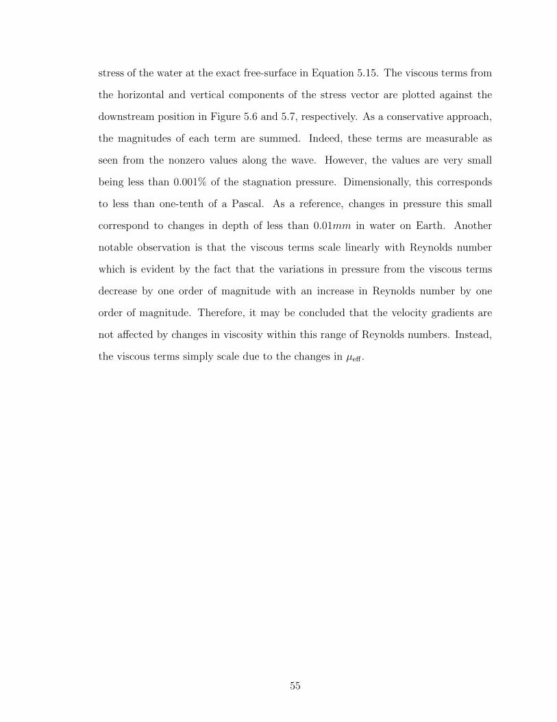
stress of the water at the exact free-surface in Equation 5.15. The viscous terms from
the horizontal and vertical components of the stress vector are plotted against the
downstream position in Figure 5.6 and 5.7, respectively. As a conservative approach,
the magnitudes of each term are summed. Indeed, these terms are measurable as
seen from the nonzero values along the wave. However, the values are very small
being less than 0.001% of the stagnation pressure. Dimensionally, this corresponds
to less than one-tenth of a Pascal. As a reference, changes in pressure this small
correspond to changes in depth of less than 0.01mm in water on Earth. Another
notable observation is that the viscous terms scale linearly with Reynolds number
which is evident by the fact that the variations in pressure from the viscous terms
decrease by one order of magnitude with an increase in Reynolds number by one
order of magnitude. Therefore, it may be concluded that the velocity gradients are
not affected by changes in viscosity within this range of Reynolds numbers. Instead,
the viscous terms simply scale due to the changes in µeff .
55
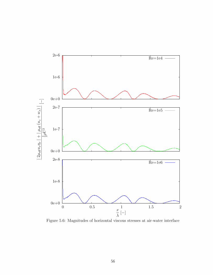
0e+0
1e-6
2e-6Re=1e4
0e+0
1e-7
2e-7
|2µ
effuxη x|+|µ
eff(u
z+wx)|
1 2ρU
2[−
]
Re=1e5
0e+0
1e-8
2e-8
0 0.5 1 1.5 2x
λ[−]
Re=1e6
Figure 5.6: Magnitudes of horizontal viscous stresses at air-water interface
56
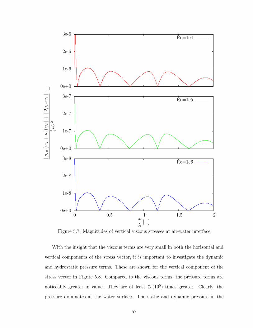
0e+0
1e-6
2e-6
3e-6Re=1e4
0e+0
1e-7
2e-7
3e-7
|µeff
(wx
+uz)η x|+|2µ
effwz|
1 2ρU
2[−
]
Re=1e5
0e+0
1e-8
2e-8
3e-8
0 0.5 1 1.5 2x
λ[−]
Re=1e6
Figure 5.7: Magnitudes of vertical viscous stresses at air-water interface
With the insight that the viscous terms are very small in both the horizontal and
vertical components of the stress vector, it is important to investigate the dynamic
and hydrostatic pressure terms. These are shown for the vertical component of the
stress vector in Figure 5.8. Compared to the viscous terms, the pressure terms are
noticeably greater in value. They are at least O (105) times greater. Clearly, the
pressure dominates at the water surface. The static and dynamic pressure in the
57

horizontal component of the stress vector are at most 10% of the vertical component,
occurring where the wave slope is greatest, ηx ≈ 0.1. It is also important to note that
the dynamic pressure is nearly identical to the hydrostatic pressure. Not only does
-0.4
-0.2
0.0
0.2
0.4hydrodynamic
hydrostatic
-0.4
-0.2
0.0
0.2
0.4
p1 2ρU
2,ρgη
1 2ρU
2[−
]
-0.4
-0.2
0.0
0.2
0.4
0 0.5 1 1.5 2x
λ[−]
Figure 5.8: Hydrodynamic and hydrostatic pressure at water surface for Re=1e4(top), Re=1e5 (middle), and Re=1e6 (bottom)
this coincide with the small viscous values previously discussed, but it also shows
the validity of employing an inviscid, zero total pressure condition in the vertical
58
direction. Indeed, this is the boundary condition solved with the linearized URANS
method:
p = ρgη (5.18)
Satisfying a pressure boundary condition on an exact free-surface requires the pressure
from both the horizontal and vertical component of the stress vector. However, the
linearized URANS method does not account for the horizontal component because
the wave elevations are approximated on a flat free-surface with a normal vector
continuously aligned with the z-axis. This approximation is valid for small wave
heights that do not deviate far from the z = 0 calm-water surface. Figure 5.9,
demonstrates this by comparing the wave elevations obtained with the VOF method
as well as those obtained by replicating the experiment with the linearized URANS
method. Only the results from the Reynolds number Re = 1e4 are compared. In
addition, at the transom the linearized URANS method uses the free-surface elevation
and pressure which coincide with the fully ventilated scenario, η = −0.25m and
p = −2452.5Pa. Due to the fixed-value pressure condition, a zero normal-gradient
condition is imposed on velocity. However, the bottom, or keel, maintains a no-slip
boundary condition. It is only the back face of the transom that requires special
consideration with the linear method. Although the two methods do not compute
wave elevations which are entirely agreeable, the results are qualitatively similar.
Those computed on z = 0 show slightly lower values at both wave crests and troughs
compared to the nonlinear results. There is also a difference in wave length, however
the linear simulations show a length which is closer to the estimated value, 2πFr2TT ≈
14.1m.
The comparison of nonlinear and linear kinematic free-surface boundary condi-
tions appears in Figure 5.10. Each curve represents data from the VOF solution only
and is normalized by U . The linear condition is computed with the constant inlet
velocity, U = 4.7m/s, whereas the nonlinear condition uses the actual horizontal
59

-1.4
-0.7
0.0
0.7
1.4
0 0.5 1 1.5 2
η T[−
]
x
λ[−]
VOFLin. URANS
Figure 5.9: Wave elevations using VOF and linerized URANS for FrT = 3 andRe = 1e4
component of velocity, u, from the solution. Lastly, w is the actual vertical compo-
nent of velocity. There is a slight difference between both conditions and the vertical
velocity along the majority of the wave. This difference decreases downstream, and
on the whole all three velocities are quite similar. Most importantly, the difference
between the linear and nonlinear conditions is very small, demonstrating that the
linear kinematic condition used with the linearized URANS method is suitable, in a
body-fixed reference frame:
w = Uηx (5.19)
It is interesting that the linear kinematic condition agrees well with the vertical
velocity at the water surface. One may not expect this to be the case when a surface-
piercing body in uniform flow possesses a boundary layer. And, in the case of a
ventilated transom stern, the boundary layer is shed at the surface of the water. So,
vorticity may be prominent at the wave surface. An explanation can be found in
Figure 5.11, which is colored by the absolute value of the vorticity in the y-direction
normalized byU
l. The lowest Reynolds number is considered, Re = 1e4, which
corresponds to the greatest viscous stresses for the range of Reynolds numbers studied.
60
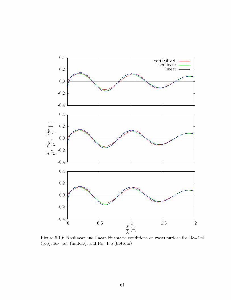
-0.4
-0.2
0.0
0.2
0.4vertical vel.
nonlinearlinear
-0.4
-0.2
0.0
0.2
0.4
w U,uη x U,Uη x U
[−]
-0.4
-0.2
0.0
0.2
0.4
0 0.5 1 1.5 2x
λ[−]
Figure 5.10: Nonlinear and linear kinematic conditions at water surface for Re=1e4(top), Re=1e5 (middle), and Re=1e6 (bottom)
61
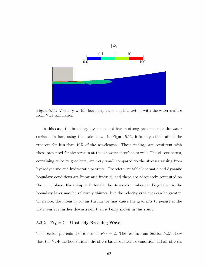
0.1 1 10
| ωy |
0.01 100
Figure 5.11: Vorticity within boundary layer and interaction with the water surfacefrom VOF simulation
In this case, the boundary layer does not have a strong presence near the water
surface. In fact, using the scale shown in Figure 5.11, it is only visible aft of the
transom for less than 10% of the wavelength. These findings are consistent with
those presented for the stresses at the air-water interface as well. The viscous terms,
containing velocity gradients, are very small compared to the stresses arising from
hydrodynamic and hydrostatic pressure. Therefore, suitable kinematic and dynamic
boundary conditions are linear and inviscid, and these are adequately computed on
the z = 0 plane. For a ship at full-scale, the Reynolds number can be greater, so the
boundary layer may be relatively thinner, but the velocity gradients can be greater.
Therefore, the intensity of this turbulence may cause the gradients to persist at the
water surface further downstream than is being shown in this study.
5.2.2 FrT = 2 – Unsteady Breaking Wave
This section presents the results for FrT = 2. The results from Section 5.2.1 show
that the VOF method satisfies the stress balance interface condition and air stresses
62
are negligible, so only the free-surface assumption is evaluated in this section. The
fundamental wavelength for this flow is λ ≈ 6.3m. As with the steady wave case, this
corresponds to an intermediate water depth, but the boundary condition used at the
bottom does not enforce a no-penetration condition. At this Froude number, an un-
steady breaking wave occurs aft of the transom. As such, a number of considerations
must be made to appropriately convey important flow features. First, the wave slope
varies from 0 → ∞, so the expression of the normal vector uses a standard global
description:
n = qi+ sk (5.20)
This results in an alternative description of the total stress vector:
σ · n =
(p− Fr−2η) q − 2Re−1uxq +Re−1 (uz + wx) s
− (p− Fr−2η) s − Re−1 (wx + uz) q + 2Re−1wzs
(5.21)
The magnitudes of the viscous terms are again summed within each component
of Equation 5.21 for a conservative approach to investigate the viscous effects at the
free-surface. Then, the hydrodynamic and hydrostatic pressures are presented, pnz
and ρgηnz, from the vertical component of the stress vector. The simulations are
two-dimensional, but a slight rotation is performed about the x−axis to improve
visualization of the iso-surfaces. For a three-dimensional investigation of interface
stresses under breaking wave conditions see Filip (2013).
63
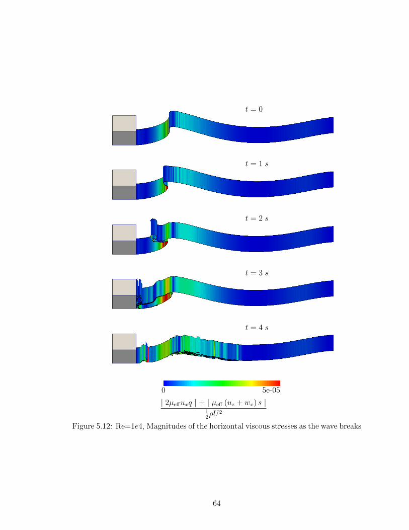
t = 0
t = 1 s
t = 2 s
t = 3 s
0 5e-05
t = 4 s
| 2µeffuxq | + | µeff (uz + wx) s |12ρU2
Figure 5.12: Re=1e4, Magnitudes of the horizontal viscous stresses as the wave breaks
64
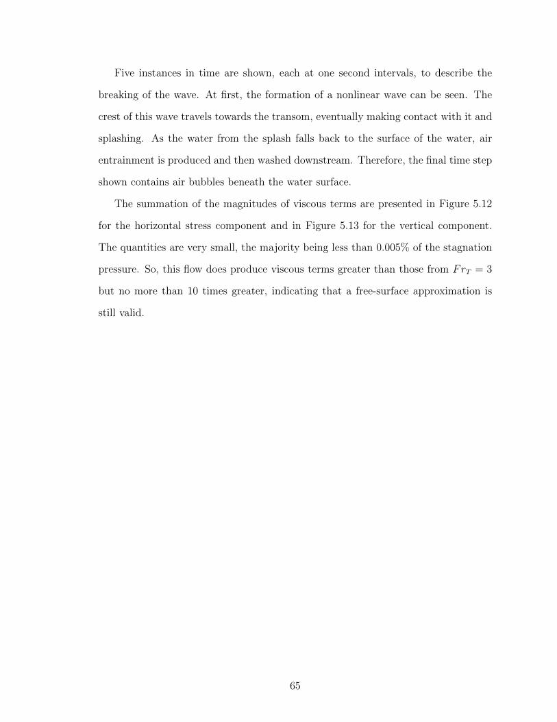
Five instances in time are shown, each at one second intervals, to describe the
breaking of the wave. At first, the formation of a nonlinear wave can be seen. The
crest of this wave travels towards the transom, eventually making contact with it and
splashing. As the water from the splash falls back to the surface of the water, air
entrainment is produced and then washed downstream. Therefore, the final time step
shown contains air bubbles beneath the water surface.
The summation of the magnitudes of viscous terms are presented in Figure 5.12
for the horizontal stress component and in Figure 5.13 for the vertical component.
The quantities are very small, the majority being less than 0.005% of the stagnation
pressure. So, this flow does produce viscous terms greater than those from FrT = 3
but no more than 10 times greater, indicating that a free-surface approximation is
still valid.
65
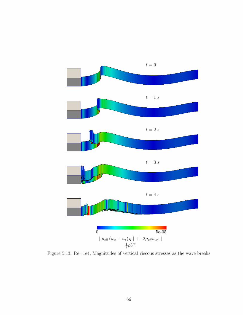
t = 0
t = 1 s
t = 2 s
t = 3 s
0 5e-05
t = 4 s
| µeff (wx + uz) q | + | 2µeffwzs |12ρU2
Figure 5.13: Re=1e4, Magnitudes of vertical viscous stresses as the wave breaks
66
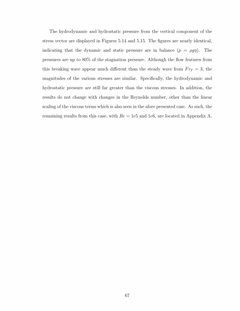
The hydrodynamic and hydrostatic pressure from the vertical component of the
stress vector are displayed in Figures 5.14 and 5.15. The figures are nearly identical,
indicating that the dynamic and static pressure are in balance (p = ρgη). The
pressures are up to 80% of the stagnation pressure. Although the flow features from
this breaking wave appear much different than the steady wave from FrT = 3, the
magnitudes of the various stresses are similar. Specifically, the hydrodynamic and
hydrostatic pressure are still far greater than the viscous stresses. In addition, the
results do not change with changes in the Reynolds number, other than the linear
scaling of the viscous terms which is also seen in the afore presented case. As such, the
remaining results from this case, with Re = 1e5 and 1e6, are located in Appendix A.
67
t = 0
t = 1 s
t = 2 s
t = 3 s
0
-0.5 0.8
t = 4 s
ps12ρU2
Figure 5.14: Re=1e4, Hydrodynamic pressure as the wave breaks
68

t = 0
t = 1 s
t = 2 s
t = 3 s
0
-0.5 0.8
t = 4 s
ρgηs12ρU2
Figure 5.15: Re=1e4, Hydrostatic pressure as the wave breaks
The viscous stresses are small, but the use of a linearized free-surface boundary
condition still raises questions as to whether this case can be approximated on the
z = 0 plane. In order to determine this possibility, the linearized URANS method
is used to replicate the experiment. The free-surface elevation and pressure are set
to the bottom of the transom, η = −0.25m and p = −5517.5Pa. This is the same
69
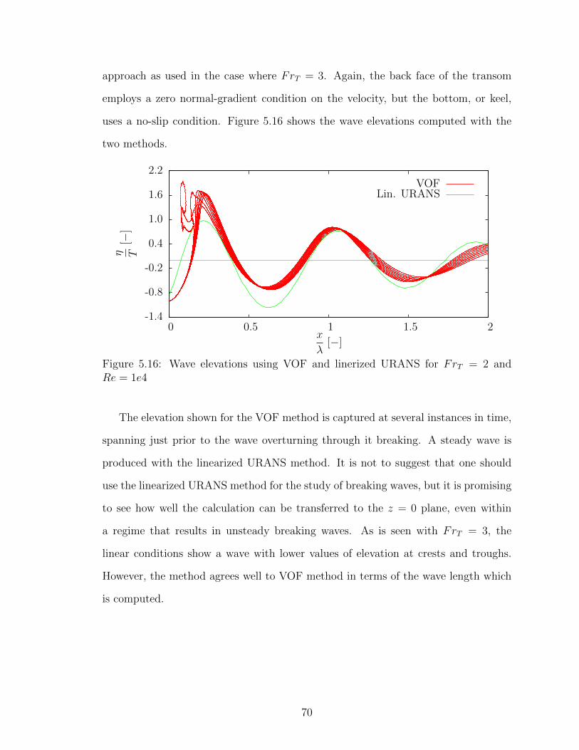
approach as used in the case where FrT = 3. Again, the back face of the transom
employs a zero normal-gradient condition on the velocity, but the bottom, or keel,
uses a no-slip condition. Figure 5.16 shows the wave elevations computed with the
two methods.
-1.4
-0.8
-0.2
0.4
1.0
1.6
2.2
0 0.5 1 1.5 2
η T[−
]
x
λ[−]
VOFLin. URANS
Figure 5.16: Wave elevations using VOF and linerized URANS for FrT = 2 andRe = 1e4
The elevation shown for the VOF method is captured at several instances in time,
spanning just prior to the wave overturning through it breaking. A steady wave is
produced with the linearized URANS method. It is not to suggest that one should
use the linearized URANS method for the study of breaking waves, but it is promising
to see how well the calculation can be transferred to the z = 0 plane, even within
a regime that results in unsteady breaking waves. As is seen with FrT = 3, the
linear conditions show a wave with lower values of elevation at crests and troughs.
However, the method agrees well to VOF method in terms of the wave length which
is computed.
70

5.2.3 FrT = 0.2 – Low Froude Number Regime
This section contains the results for the set of data where FrT = 0.2. A fundamental
wavelength of λ ≈ 0.063m is associated with this regime. The normal unit vector, n,
is expressed in terms of the water surface elevation, η. Figure 5.17 shows the water
surface elevations. Changes in Reynolds number do not significantly change the water
surface elevation.
-0.2
-0.1
0.0
0.1
0.2
0 2 4 6 8 10
η T[−
]
x
λ[−]
Re=1e4Re=1e5Re=1e6
Figure 5.17: Wave elevations
For this discussion, the viscous terms are shown individually for both the horizon-
tal and vertical components of the stress vector in Figure 5.18. The terms are very
small. The static nature of this case presents difficulties with the smearing of the
interface. Near the back face of the transom, the fluid does not adequately convect
downstream to produce a crisp interface. Instead, a large interface exists, spanning
several cells, and contains a slurry of fluid which is much denser than air. As such,
using a rigorous phase-indicator variable cutoff of α = 0.99 results in a water surface
elevation which is too low. Therefore, a more suitable value of α = 0.5 is used for the
data presented at this low Froude number regime.
71
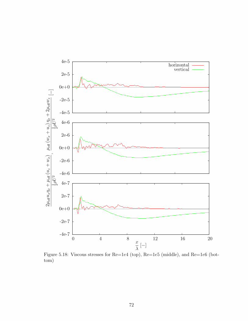
-4e-5
-2e-5
0e+0
2e-5
4e-5horizontal
vertical
-4e-6
-2e-6
0e+0
2e-6
4e-6
2µeffuxη x
+µ
eff(u
z+wx)
1 2ρU
2,µ
eff(w
x+uz)η x
+2µ
effwz
1 2ρU
2[−
]
-4e-7
-2e-7
0e+0
2e-7
4e-7
0 4 8 12 16 20x
λ[−]
Figure 5.18: Viscous stresses for Re=1e4 (top), Re=1e5 (middle), and Re=1e6 (bot-tom)
72
Figure 5.19 presents the hydrodynamic and hydrostatic pressures from the verti-
cal component of the stress vector. Since this case is largely governed by hydrostatic
pressure, the stress scale used for non-dimensionalization is ρgT . Indeed, air-water
interface is disturbed little, which is reflected by the small static and dynamic pres-
sures at the water surface. Also, the dynamic and static pressures are in balance.
They are at most roughly 1% different in relation to the stress scale, ρgT . The nearly
flat interface causes pressures from the horizontal component of the stress vector to
be even smaller, and, therefore, they are not plotted.
73

-0.10
-0.05
0.00
0.05
0.10hydrodynamic
hydrostatic
-0.10
-0.05
0.00
0.05
0.10
p
ρgT,ρgη
ρgT
[−]
-0.10
-0.05
0.00
0.05
0.10
0 4 8 12 16 20x
λ[−]
Figure 5.19: Hydrodynamic and hydrostatic pressure from vertical component ofstress at water surface for Re=1e4 (top), Re=1e5 (middle), and Re=1e6 (bottom)
74
The comparison of the linear and nonlinear kinematic conditions can be seen in
Figure 5.20. The nonlinear condition agrees slightly better with the vertical veloc-
ity from the solution close to the transom than the linear condition. Downstream,
both methods perform similarly. Any differences between the linear, nonlinear, and
actual values are small, being at most roughly 2% different in relation to the inlet
velocity, U . Figure 5.21 displays the absolute value of vorticity in the y-direction.
The recirculation region just aft of the transom corresponds to the region where the
linear kinematic condition shows the largest difference. Here, the fluid velocity is
less than the free-stream velocity, so the linear kinematic condition, using U , dis-
agrees with the nonlinear condition. Still, employing the linearized condition results
in a very agreeable solution to the free-surface elevation as depicted in Figure 5.22,
which compares the VOF solution to the linearized URANS solution. At this Froude
number, the linearized URANS simulation uses the same boundary conditions as the
fully nonlinear approach. The back face of the transom uses a zero normal-gradient
for the pressure and free-surface elevation. The velocity satisfies a no-slip boundary
condition everywhere on the transom.
75
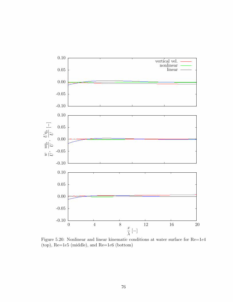
-0.10
-0.05
0.00
0.05
0.10vertical vel.
nonlinearlinear
-0.10
-0.05
0.00
0.05
0.10
w U,uη x U,Uη x U
[−]
-0.10
-0.05
0.00
0.05
0.10
0 4 8 12 16 20x
λ[−]
Figure 5.20: Nonlinear and linear kinematic conditions at water surface for Re=1e4(top), Re=1e5 (middle), and Re=1e6 (bottom)
76

0.1 1 10
| ωy |
0.01 100
Figure 5.21: Vorticity within boundary layer and interaction with the water surface
-0.10
-0.05
0.00
0.05
0.10
0 2 4 6 8 10
η T[−
]
x
λ[−]
VOFLin. URANS
Figure 5.22: Wave elevations using VOF and linerized URANS for FrT = 0.2 andRe = 1e4
5.3 Summary of Findings
The two-dimensional viscous interface study allows for several important conclusions.
First, the stress-balance of the air-water interface condition is satisfied using the
VOF method. Any differences in stress from the air and water are very small and
can be attributed to the rigor with which the phase-indicator variable thresholds are
77

implemented. In an attempt to measure values which are very nearly in air and water,
α = 0.01 and α = 0.99 are chosen. This produces a finite gap between the two fluids
where the interface resides. In addition, the magnitude of the stress in each fluid at the
interface is shown to be very small, suggesting that only consideration of the stresses
in the water through the free-surface approximation is an appropriate assumption.
From here, this free-surface condition is evaluated with nine combinations of Froude
and Reynolds numbers.
The ventilated transom produced with FrT = 3 results in a steady, non-breaking
wave. A conservative approach is taken to determine the effect of the viscous terms
in the free-surface condition by summing the magnitude of each term. It is shown
that this summation is still very small and the viscous terms can be neglected. The
hydrodynamic and hydrostatic pressure terms dominate in the horizontal and verti-
cal components of the stress vector equation. Within these, the vertical terms are
approximately ten times larger than the horizontal terms. Therefore, a zero total
pressure condition in the vertical direction is suitable for the dynamic free-surface
boundary condition. The kinematic condition is also studied with results showing
little difference between a linear and a nonlinear approach, both of which agree well
with the vertical velocity at the surface along the entire wave.
An unsteady breaking wave is produced at FrT = 2. This wave causes the venti-
lation of the transom to oscillate from fully to partially ventilated as the wave breaks
and splashes against the back face of the transom. Iso-surfaces are used to convey
important features of the data. The conservative summation of magnitudes is again
taken when visualizing the viscous terms in the horizontal and vertical components
of the stress vector. The effects of viscosity are larger in magnitude than the steady
wave case, but they are still very small. It is clear that the hydrodynamic and hydro-
static pressures dominate the zero total stress condition, and they are very nearly in
balance. A reasonable solution to this unsteady flow, transferred to the z = 0 plane,
78
is shown.
The final case addresses the Froude number FrT = 0.2 in which essentially no
wave is generated. The viscous terms in the horizontal and vertical components of
the stress vector are once again very small, being on the order of those from the
case where FrT = 2. The values of the slope of the water surface, ηx, are very near
zero everywhere. Therefore, the hydrodynamic and hydrostatic pressure from the
horizontal component of the stress vector are practically zero. In addition, the static
nature of the flow produces dynamic and static pressures in the vertical component of
the stress vector which are very small. These are normalized by a static stress scale,
ρgT . Studying the kinematic condition shows the linear approach produces a small
difference in the prediction of vertical velocity within the recirculation region just aft
of the transom. The nonlinear condition agrees well with the vertical velocity in this
region. Still, the linearized URANS method produces results which are very similar
to those obtained with the fully nonlinear VOF method.
79
CHAPTER VI
Maneuvering Tests
This section presents results using the linearized URANS method on two variations of
the David Taylor Model Basin (DTMB) 5415 destroyer hull form. The first variation
is the DTMB 5415, which is unappended with the exception of bilge keels. In the lit-
erature, this is referred to as the bare hull. The second variation is the DTMB 5415M,
which is fully appended with bilge keels, stabilizer fins, five-bladed inward-rotating
propellers, spade rudders, exposed propeller shafts, and A-frame shaft brackets. This
is accordingly referred to as the appended hull.
Results are mainly focused on forces and moments in the horizontal plane. These
ship-fixed forces are an axial surge force, X, a lateral sway force, Y , and a yaw
moment about midship, N . The propeller thrust force, T , acts along the propeller
shaft axis-of-rotation. Each force and moment is presented in a dimensionless manner,
as shown in Equation 6.1.
X ′, Y ′, T ′ =X, Y, T
0.5ρU2cAo
N ′ =N
0.5ρU2cAoLpp
(6.1)
The carriage speed is denoted with Uc. The length between perpendiculars is Lpp,
and the lateral underwater area, Ao, is LppT where T is the draft.
80

Unstructured grids are used for both hulls with the native semi-automatic mesh
generator in OpenFOAM, snappyHexMesh, which allows for a hexahedron dominant
mesh as well as boundary layer prisms on hull surfaces. The hands-off nature of snap-
pyHexMesh coincides with the goal of design efficiency for this linearized method. The
Spalart-Allmaras turbulence model is used with an adaptive wall function. Simula-
tions are performed in an inertial, Earth-fixed reference frame. The linearization
restricts body-exact ship motions to those in the horizontal-plane (surge, sway, and
yaw). The rotation of propellers is performed with a sliding mesh communication,
or arbitrary mesh interface (AMI) in OpenFOAM. Details of this technology can be
found in Farrell and Maddison (2011), and an application is shown in McNaughton
et al. (2014).
6.1 DTMB 5415 - Bare Hull
Prescribed PMM tests are conducted with the DTMB 5415 bare hull. These consist
of static drift, pure sway, and pure yaw tests and are compared with experimental
data from the Iowa Institute of Hydraulic Research (IIHR) (Longo et al., 2006) and
from FORCE Technology in Denmark (Agdrup, 2004). The IIHR model is fixed at
the dynamic sinkage and trim, whereas the FORCE Technology model is free to sink
and trim. The hull used in the IIHR physical experiments is displayed in Figure 6.1,
and the model characteristics are shown in Table 6.1.
81

Figure 6.1: DTMB 5415 bare hull model from IIHR experiments. Top photographshows the keel and both bilge keels
Table 6.1: IIHR DTMB 5415 model principle characteristics
Item Symbol Value UnitScale factor λ 46.588 –Length Lpp 3.048 mWaterline length Lwl 3.052 mBeam Bwl 0.410 mDraft T 0.136 mMass m 83.35 kgLateral area Ao 0.415 m2
Only the pure sway and pure yaw maneuvers are compared to experimental data
from FORCE Technology in Denmark. The hull used in these experiments is shown
in Figure 6.2, and the model characteristics appear in Table 6.2.
Figure 6.2: FORCE DTMB 5415 bare hull model
82
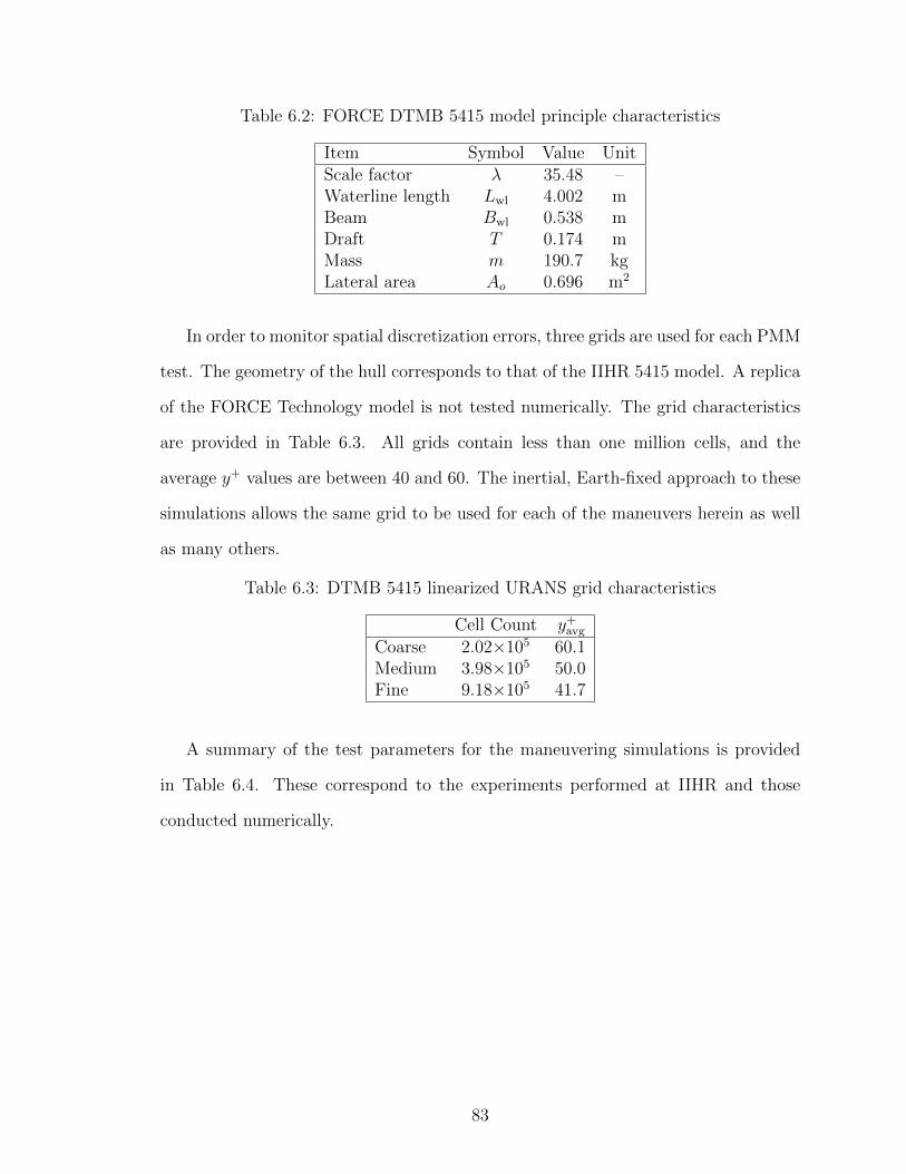
Table 6.2: FORCE DTMB 5415 model principle characteristics
Item Symbol Value UnitScale factor λ 35.48 –Waterline length Lwl 4.002 mBeam Bwl 0.538 mDraft T 0.174 mMass m 190.7 kgLateral area Ao 0.696 m2
In order to monitor spatial discretization errors, three grids are used for each PMM
test. The geometry of the hull corresponds to that of the IIHR 5415 model. A replica
of the FORCE Technology model is not tested numerically. The grid characteristics
are provided in Table 6.3. All grids contain less than one million cells, and the
average y+ values are between 40 and 60. The inertial, Earth-fixed approach to these
simulations allows the same grid to be used for each of the maneuvers herein as well
as many others.
Table 6.3: DTMB 5415 linearized URANS grid characteristics
Cell Count y+avg
Coarse 2.02×10⁵ 60.1Medium 3.98×10⁵ 50.0Fine 9.18×10⁵ 41.7
A summary of the test parameters for the maneuvering simulations is provided
in Table 6.4. These correspond to the experiments performed at IIHR and those
conducted numerically.
83

Table 6.4: DTMB 5415 maneuvering test parameters
Item Symbol Value UnitCarriage speed Uc 1.531 m/sFroude num. Fr 0.280Reynolds num. Re 4.464×10⁶
Gravity g 9.81 m/s2
Water density ρ 1000 kg/m3
Water viscosity ν 1.00×10⁻⁶ m2/s
Static driftDrift angle β 10 deg
Pure swaySway amplitude η0 0.317 mSway frequency Npmm 8.021 min−1
Pure yawSway amplitude η0 0.327 mYaw amplitude ψ0 10.2 degYaw frequency Npmm 8.021 min−1
6.1.1 Static Drift
The static drift simulations are compared to experimental data from IIHR. Mesh
motion is governed by Equation 6.2 for the static drift test, where β = 10◦:
β = − tan−1(vu
)Uc =
√u2 + v2
(6.2)
The steady nature of the static drift test presents an opportunity to perform a
grid convergence study with the linearized URANS approach because determination
of the time-averaged values is straight-forward compared to the unsteady forces of the
dynamic cases. First, the ASME uncertainty procedure is used to find an observed
order of accuracy, p (ASME, 2008). However, the ASME procedure is based on
Richardson extrapolation, where the observed order of accuracy should be no greater
than p = 2. Since unrealistic super-convergence (p > 2) is observed in this static drift
84
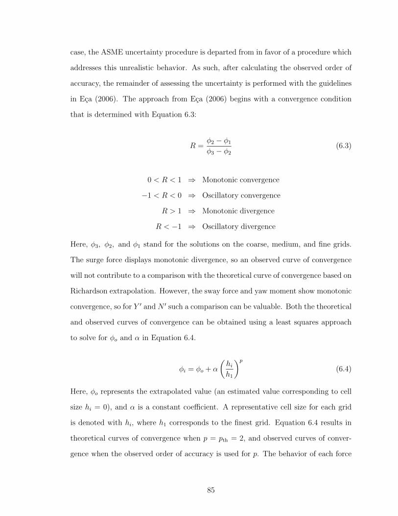
case, the ASME uncertainty procedure is departed from in favor of a procedure which
addresses this unrealistic behavior. As such, after calculating the observed order of
accuracy, the remainder of assessing the uncertainty is performed with the guidelines
in Eca (2006). The approach from Eca (2006) begins with a convergence condition
that is determined with Equation 6.3:
R =φ2 − φ1
φ3 − φ2
(6.3)
0 < R < 1 ⇒ Monotonic convergence
−1 < R < 0 ⇒ Oscillatory convergence
R > 1 ⇒ Monotonic divergence
R < −1 ⇒ Oscillatory divergence
Here, φ3, φ2, and φ1 stand for the solutions on the coarse, medium, and fine grids.
The surge force displays monotonic divergence, so an observed curve of convergence
will not contribute to a comparison with the theoretical curve of convergence based on
Richardson extrapolation. However, the sway force and yaw moment show monotonic
convergence, so for Y ′ and N ′ such a comparison can be valuable. Both the theoretical
and observed curves of convergence can be obtained using a least squares approach
to solve for φo and α in Equation 6.4.
φi = φo + α
(hih1
)p(6.4)
Here, φo represents the extrapolated value (an estimated value corresponding to cell
size hi = 0), and α is a constant coefficient. A representative cell size for each grid
is denoted with hi, where h1 corresponds to the finest grid. Equation 6.4 results in
theoretical curves of convergence when p = pth = 2, and observed curves of conver-
gence when the observed order of accuracy is used for p. The behavior of each force
85
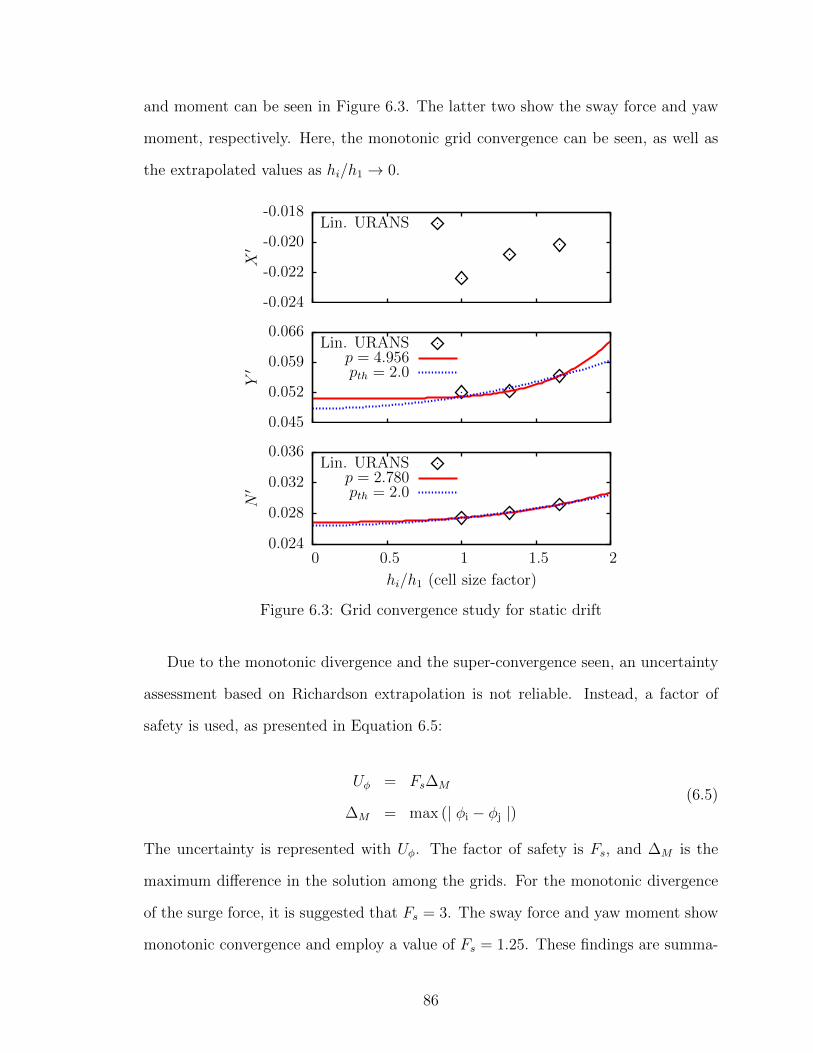
and moment can be seen in Figure 6.3. The latter two show the sway force and yaw
moment, respectively. Here, the monotonic grid convergence can be seen, as well as
the extrapolated values as hi/h1 → 0.
-0.024
-0.022
-0.020
-0.018
X′
Lin. URANS
0.045
0.052
0.059
0.066
Y′
Lin. URANSp = 4.956pth = 2.0
0.024
0.028
0.032
0.036
0 0.5 1 1.5 2
N′
hi/h1 (cell size factor)
Lin. URANSp = 2.780pth = 2.0
Figure 6.3: Grid convergence study for static drift
Due to the monotonic divergence and the super-convergence seen, an uncertainty
assessment based on Richardson extrapolation is not reliable. Instead, a factor of
safety is used, as presented in Equation 6.5:
Uφ = Fs∆M
∆M = max (| φi − φj |)(6.5)
The uncertainty is represented with Uφ. The factor of safety is Fs, and ∆M is the
maximum difference in the solution among the grids. For the monotonic divergence
of the surge force, it is suggested that Fs = 3. The sway force and yaw moment show
monotonic convergence and employ a value of Fs = 1.25. These findings are summa-
86
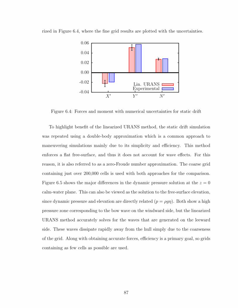
rized in Figure 6.4, where the fine grid results are plotted with the uncertainties.
-0.04
-0.02
0.00
0.02
0.04
0.06
X ′ Y ′ N ′
Lin. URANSExperimental
Figure 6.4: Forces and moment with numerical uncertainties for static drift
To highlight benefit of the linearized URANS method, the static drift simulation
was repeated using a double-body approximation which is a common approach to
maneuvering simulations mainly due to its simplicity and efficiency. This method
enforces a flat free-surface, and thus it does not account for wave effects. For this
reason, it is also referred to as a zero-Froude number approximation. The coarse grid
containing just over 200,000 cells is used with both approaches for the comparison.
Figure 6.5 shows the major differences in the dynamic pressure solution at the z = 0
calm-water plane. This can also be viewed as the solution to the free-surface elevation,
since dynamic pressure and elevation are directly related (p = ρgη). Both show a high
pressure zone corresponding to the bow wave on the windward side, but the linearized
URANS method accurately solves for the waves that are generated on the leeward
side. These waves dissipate rapidly away from the hull simply due to the coarseness
of the grid. Along with obtaining accurate forces, efficiency is a primary goal, so grids
containing as few cells as possible are used.
87

Figure 6.5: Coarse grid pressure comparison of linearized URANS (top) and double-body (bottom) for static drift β = 10◦
To give a more quantitative comparison, the forces obtained using both techniques
are shown in Figure 6.6. Both methods perform well in predicting the surge force
obtained with the physical experiments. However, the zero Froude approach shows a
difference of over 20% for both the sway force and yaw moment. On the other hand,
the linearized URANS method still compares well to the experiments being less than
5% different in all categories.
88

-0.04
-0.02
0.00
0.02
0.04
0.06
X ′ Y ′ N ′
Lin. URANSExperimentalDouble-body
Figure 6.6: Static drift for linearized URANS and Double-body
The computational expense of each method is also important. The linearized
URANS method requires 10% more computing time than the double-body simu-
lation. Specifically, 9.29 hours vs. 8.43 hours on 12 processors for 60 seconds of
simulated time. For a slightly greater expense, the improved accuracy of accounting
for first-order wave effects is significant and still possible to obtain with workstation
computing.
6.1.2 Pure Sway
Results for the pure sway test are compared to both IIHR and FORCE Technology
experiments. The mesh motion for the pure sway test is shown in Equation 6.6:
ηsway = −η0 sin
(2πNPMM
60t
)(6.6)
The numerical carriage velocity is a constant Uc = 1.531m/s, and the corresponding
sway motion period is 7.48s. In addition to the experimental data from the two
testing facilities, results from a fully nonliner method are provided from Miller (2008).
These are obtained with CFDShip-Iowa which uses a level-set method to solve for
the location of the water surface. One set of CFDShip-Iowa results correspond to
simulations performed with a domain that is consistent with the dimensions of the
89
tank at IIHR. The second set corresponds to the FORCE Technology tank dimensions.
As such, results are grouped by testing facility and the corresponding CFDShip-Iowa
data. The linearized URANS results are the same within these two groups. The fully-
nonlinear grids employ just over 4.5 million cells. Table 6.5 shows the dimensions of
the two tanks.
Table 6.5: Comparison of IIHR and FORCE tank dimensions
Length Width Depth [m]IIHR 100 3 3FORCE 240 12 5.5
Forces and moments compared to IIHR data over one PMM period are displayed
in Figure 6.7. The surge force from the linearized URANS results does not possess the
amount of variation that the experimental signal does, but the time-averaged values
of each are quite similar. The time-averaged values are in slightly worse agreement for
the CFDShip-Iowa results. The linear predictions of sway force show a noticeable shift
with respect to the experimental data, but they are otherwise in good agreement. The
CFDShip-Iowa prediction is in excellent agreement with the experiments. This may
indicate that the physical tank boundaries affect the forces and need to be modeled
numerically as in the CFDShip-Iowa results. Indeed, the tank is only 3m wide, so the
sway amplitude of η0 = 0.317m causes the model to traverse over 20% of the tank
width. Lastly, all methods display good agreement of the predicted yaw moment.
Forces and moments compared to FORCE Technology data over one PMM period
are displayed in Figure 6.8. The time-averaged values of the linearized URANS surge
force are in decent agreement with experimental data. Fully-nonlinear data shows
great agreement, even with prediction of the variation in amplitude of the surge
force. The linear predictions of sway force again show a noticeable phase shift with
respect to the experimental data, but they are otherwise in close agreement, and
the CFDShip-Iowa prediction is very close to the experiments. Each method shows
90
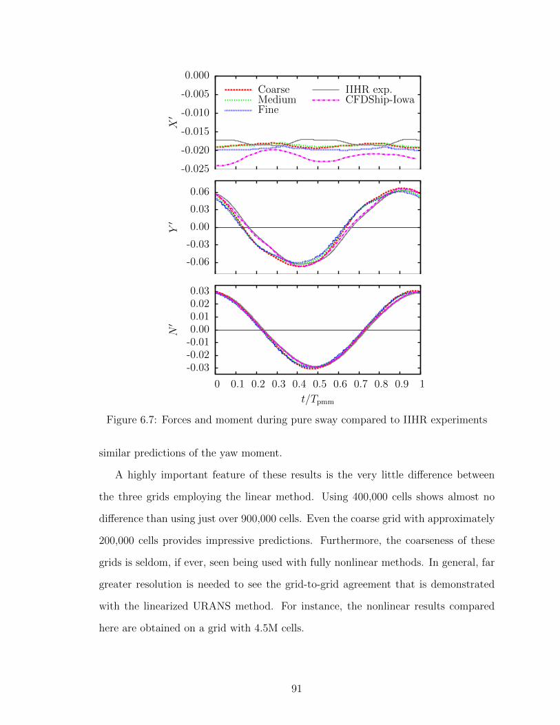
-0.025
-0.020
-0.015
-0.010
-0.005
0.000
X′
CoarseMediumFine
IIHR exp.CFDShip-Iowa
-0.06
-0.03
0.00
0.03
0.06
Y′
-0.03-0.02-0.010.000.010.020.03
0 0.1 0.2 0.3 0.4 0.5 0.6 0.7 0.8 0.9 1
N′
t/Tpmm
Figure 6.7: Forces and moment during pure sway compared to IIHR experiments
similar predictions of the yaw moment.
A highly important feature of these results is the very little difference between
the three grids employing the linear method. Using 400,000 cells shows almost no
difference than using just over 900,000 cells. Even the coarse grid with approximately
200,000 cells provides impressive predictions. Furthermore, the coarseness of these
grids is seldom, if ever, seen being used with fully nonlinear methods. In general, far
greater resolution is needed to see the grid-to-grid agreement that is demonstrated
with the linearized URANS method. For instance, the nonlinear results compared
here are obtained on a grid with 4.5M cells.
91

-0.025
-0.020
-0.015
-0.010
-0.005
0.000
X′
CoarseMediumFine
FORCE exp.CFDShip-Iowa
-0.06
-0.03
0.00
0.03
0.06
Y′
-0.03-0.02-0.010.000.010.020.03
0 0.1 0.2 0.3 0.4 0.5 0.6 0.7 0.8 0.9 1
N′
t/Tpmm
Figure 6.8: Forces and moment during pure sway compared to FORCE Technologyexperiments
6.1.3 Pure Yaw
The motion governing the pure yaw maneuver appears in Equation 6.7:
ψyaw = −ψ0 cos
(2πNPMM
60t
)ηsway = −η0 sin
(2πNPMM
60t
) (6.7)
For this test, the sway amplitude is η0 = 0.327m, and the maximum heading angle
is ψ0 = 10.2◦. As with the pure sway tests, results from both IIHR and FORCE
are shown along with CFDShip-Iowa data corresponding the the two tank dimen-
92
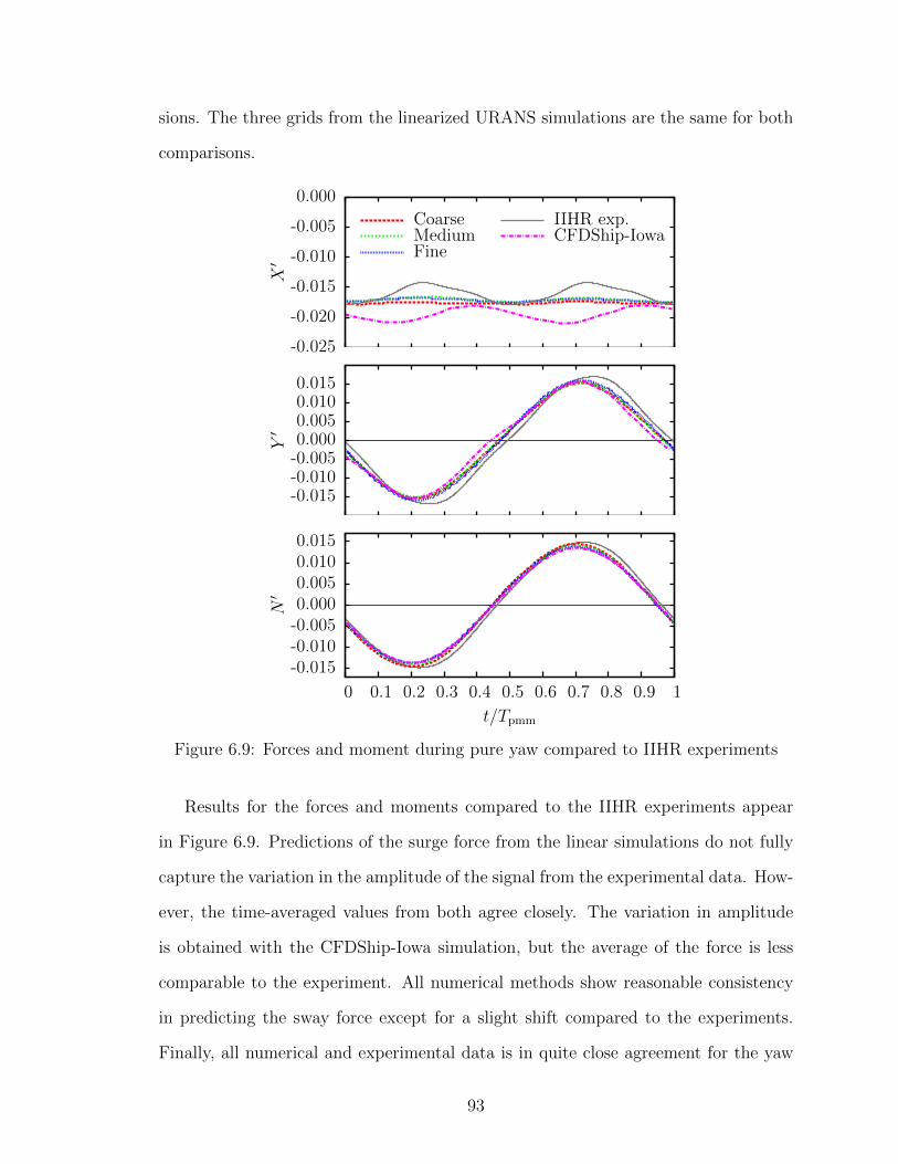
sions. The three grids from the linearized URANS simulations are the same for both
comparisons.
-0.025
-0.020
-0.015
-0.010
-0.005
0.000
X′
CoarseMediumFine
IIHR exp.CFDShip-Iowa
-0.015-0.010-0.0050.0000.0050.0100.015
Y′
-0.015-0.010-0.0050.0000.0050.0100.015
0 0.1 0.2 0.3 0.4 0.5 0.6 0.7 0.8 0.9 1
N′
t/Tpmm
Figure 6.9: Forces and moment during pure yaw compared to IIHR experiments
Results for the forces and moments compared to the IIHR experiments appear
in Figure 6.9. Predictions of the surge force from the linear simulations do not fully
capture the variation in the amplitude of the signal from the experimental data. How-
ever, the time-averaged values from both agree closely. The variation in amplitude
is obtained with the CFDShip-Iowa simulation, but the average of the force is less
comparable to the experiment. All numerical methods show reasonable consistency
in predicting the sway force except for a slight shift compared to the experiments.
Finally, all numerical and experimental data is in quite close agreement for the yaw
93
moment.
Results corresponding to FORCE Technology experiments are displayed in Fig-
ure 6.10. Far less variation is seen in the amplitude of the surge force compared to
the IIHR tank in Figure 6.9. The CFDShip-Iowa simulations show the closest predic-
tions to the experiments, but the linearized URANS data are also closely predictive.
A noticeable difference in the experimental sway force can been seen, as it shows a
larger amplitude than each numerical method. This may be because the model is
free to heave and pitch in the experiments. The linear simulations show the closest
agreement to this experimental force. Lastly, each method agrees well in predicting
the yaw moment.
94
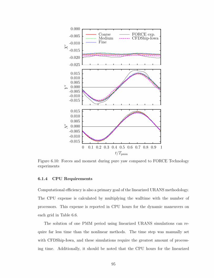
-0.025
-0.020
-0.015
-0.010
-0.005
0.000
X′
CoarseMediumFine
FORCE exp.CFDShip-Iowa
-0.015-0.010-0.0050.0000.0050.0100.015
Y′
-0.015-0.010-0.0050.0000.0050.0100.015
0 0.1 0.2 0.3 0.4 0.5 0.6 0.7 0.8 0.9 1
N′
t/Tpmm
Figure 6.10: Forces and moment during pure yaw compared to FORCE Technologyexperiments
6.1.4 CPU Requirements
Computational efficiency is also a primary goal of the linearized URANS methodology.
The CPU expense is calculated by multiplying the walltime with the number of
processors. This expense is reported in CPU hours for the dynamic maneuvers on
each grid in Table 6.6.
The solution of one PMM period using linearized URANS simulations can re-
quire far less time than the nonlinear methods. The time step was manually set
with CFDShip-Iowa, and these simulations require the greatest amount of process-
ing time. Additionally, it should be noted that the CPU hours for the linearized
95

Table 6.6: CPU hours per PMM period
Pure sway Pure yawCoarse 11.5 10.4Medium 56.3 35.8Fine 221.9 196.0CFDShip-Iowa 322 322
URANS maneuvers correspond to conservative simulations with no under-relaxation
and maximum allowable Courant numbers of just Cmax = 2. VOF simulations re-
ported in Vukcevic et al. (2014) using the IIHR model require roughly 72 CPU hours
per PMM period. This is less computationally expensive than the fine grid, but the
VOF simulations use a maximum Courant number of Cmax = 50. A similar setting
would greatly increase the speed of the linearized URANS simulations.
The low computational expense required by the linearized URANS method makes
it suitable for use on a multi-core workstation. Computing clusters are often inacces-
sible to designers. The ability to use machines already present in the workplace shows
promise that RANS-based maneuvering simulations can be brought into engineering
practice more immediately.
6.1.5 Flow Field Data
In this section, the linearized free-surface approach is used in conjunction with large
eddy simulation (LES) and a grid of approximately four million cells for the pure
sway maneuver. The turbulence model implemented is a dynamic one-equation
eddy-viscosity model. The purpose of this investigation is to determine the effect
of linearization on the flow around the hull. Results are compared to particle image
velocimetry (PIV) data from IIHR. Five categories of data are presented, all in a
ship-fixed reference frame. These are shown at four phases throughout one PMM
period, as seen in Figure 6.11. The sampling location is the same for each moment
in time and is located at x/Lpp = 0.935 from the bow. Quantities of a bow-aligned
96

axial velocity, a lateral velocity, a vertical velocity, an axial vorticity, and a turbulent
kinetic energy are examined. All values have been non-dimensionalized using the
carriage speed, U = 1.531m/s and the model length, Lpp = 3.048m.
0◦
t/TPMM = 0
45◦
t/TPMM = 0.125
90◦
t/TPMM = 0.25135◦
t/TPMM = 0.375
Figure 6.11: PIV sampling points and locations for pure sway
The effects of the linearization are most prevalent in Figure 6.12 which shows the
axial velocity. The linearization neglects the perturbation velocity which is not small
everywhere in the domain. In fact, it is equal to the ship velocity on the surface
of the hull. This results in the large difference between the experimental and LES
results. The PIV data also capture the vortex that the sonar dome generates. The
first instance of this feature is seen directly below the keel in the first contour plot of
Figure 6.12. For the most part, this vortex is not captured with the linearized LES
method. It is likely that a finer grid is necessary to more accurately resolve the flow
field data. More agreeable predictions are seen with the lateral velocity presented
in Figure 6.13. The perturbation velocity in sway is not as large as in surge, so the
effects of using a linear free-surface condition are not as noticeable. Again, the vortex
from the sonar dome is not as apparent as in the PIV data. These general conclusions
apply to the vertical velocity as well, shown in Figure 6.14. Qualitatively, the axial
vorticity in Figure 6.15 is similar to the PIV data. However, the vorticity from the
PIV shows distinct circular structures, whereas the linearized LES data are more
elongated. Again, a probable cause for this is insufficient grid resolution. Lastly, the
turbulent kinetic energy is displayed in Figure 6.16. Compared to the PIV figures,
the numerical data are rather poor, especially in the last two phases in time. This
may be due to an unresolved grid or an issue with the turbulence model.
97
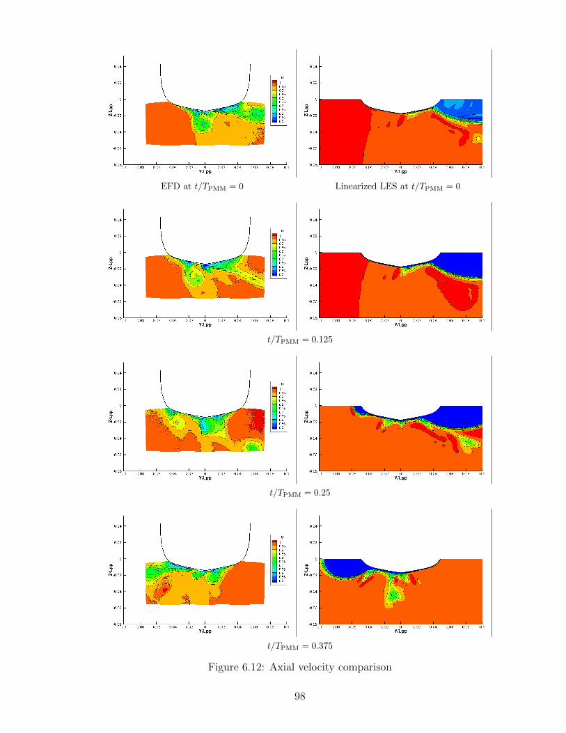
EFD at t/TPMM = 0 Linearized LES at t/TPMM = 0
t/TPMM = 0.125
t/TPMM = 0.25
t/TPMM = 0.375
Figure 6.12: Axial velocity comparison
98

EFD at t/TPMM = 0 Linearized LES at t/TPMM = 0
t/TPMM = 0.125
t/TPMM = 0.25
t/TPMM = 0.375
Figure 6.13: Lateral velocity comparison
99

EFD at t/TPMM = 0 Linearized LES at t/TPMM = 0
t/TPMM = 0.125
t/TPMM = 0.25
t/TPMM = 0.375
Figure 6.14: Vertical velocity comparison
100
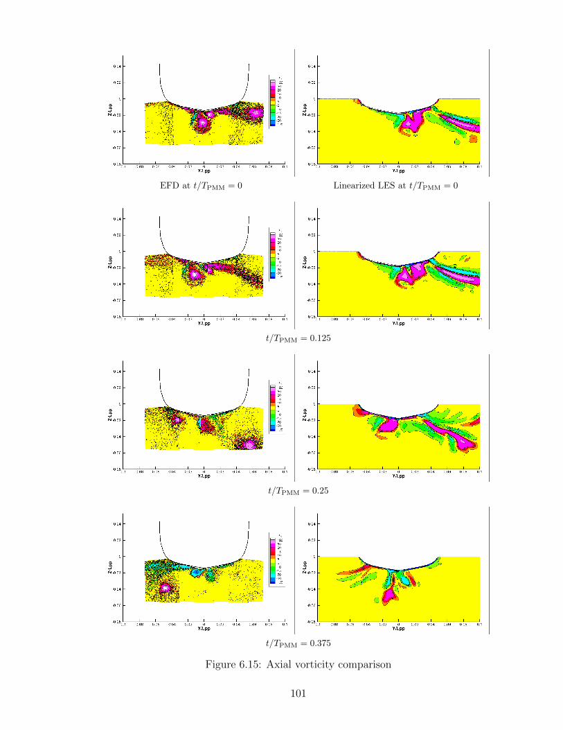
EFD at t/TPMM = 0 Linearized LES at t/TPMM = 0
t/TPMM = 0.125
t/TPMM = 0.25
t/TPMM = 0.375
Figure 6.15: Axial vorticity comparison
101

EFD at t/TPMM = 0 Linearized LES at t/TPMM = 0
t/TPMM = 0.125
t/TPMM = 0.25
t/TPMM = 0.375
Figure 6.16: Turbulent kinetic energy comparison
102
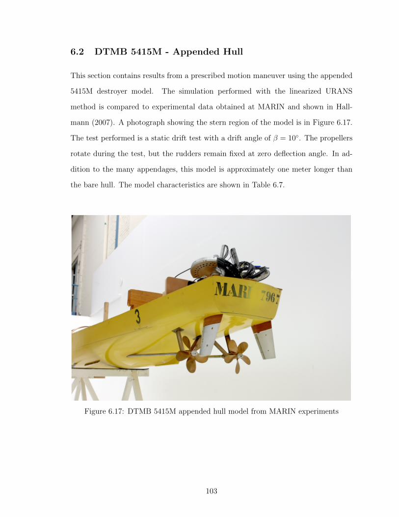
6.2 DTMB 5415M - Appended Hull
This section contains results from a prescribed motion maneuver using the appended
5415M destroyer model. The simulation performed with the linearized URANS
method is compared to experimental data obtained at MARIN and shown in Hall-
mann (2007). A photograph showing the stern region of the model is in Figure 6.17.
The test performed is a static drift test with a drift angle of β = 10◦. The propellers
rotate during the test, but the rudders remain fixed at zero deflection angle. In ad-
dition to the many appendages, this model is approximately one meter longer than
the bare hull. The model characteristics are shown in Table 6.7.
Figure 6.17: DTMB 5415M appended hull model from MARIN experiments
103
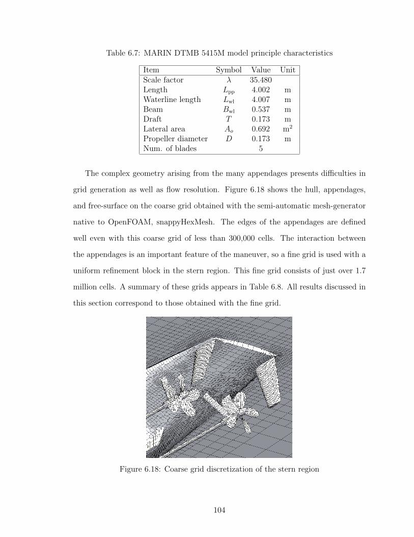
Table 6.7: MARIN DTMB 5415M model principle characteristics
Item Symbol Value UnitScale factor λ 35.480Length Lpp 4.002 mWaterline length Lwl 4.007 mBeam Bwl 0.537 mDraft T 0.173 mLateral area Ao 0.692 m2
Propeller diameter D 0.173 mNum. of blades 5
The complex geometry arising from the many appendages presents difficulties in
grid generation as well as flow resolution. Figure 6.18 shows the hull, appendages,
and free-surface on the coarse grid obtained with the semi-automatic mesh-generator
native to OpenFOAM, snappyHexMesh. The edges of the appendages are defined
well even with this coarse grid of less than 300,000 cells. The interaction between
the appendages is an important feature of the maneuver, so a fine grid is used with a
uniform refinement block in the stern region. This fine grid consists of just over 1.7
million cells. A summary of these grids appears in Table 6.8. All results discussed in
this section correspond to those obtained with the fine grid.
Figure 6.18: Coarse grid discretization of the stern region
104
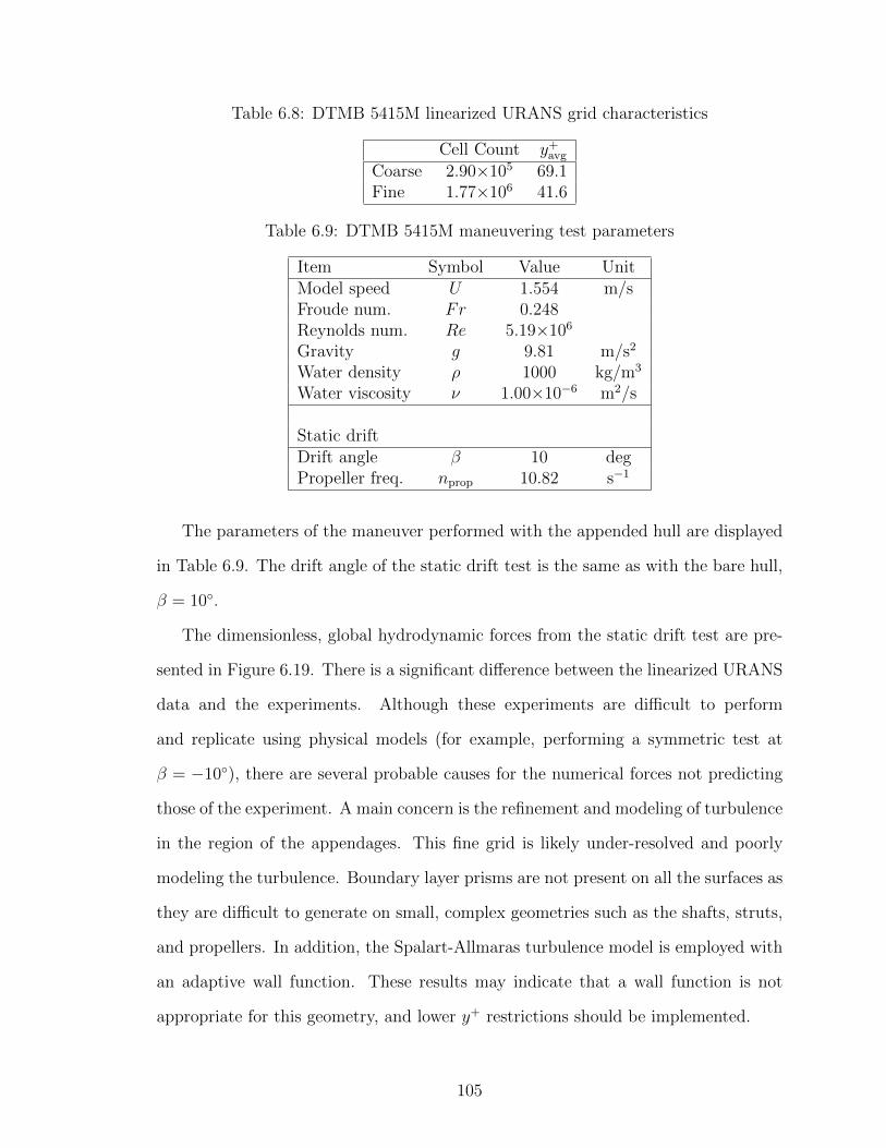
Table 6.8: DTMB 5415M linearized URANS grid characteristics
Cell Count y+avg
Coarse 2.90×10⁵ 69.1Fine 1.77×10⁶ 41.6
Table 6.9: DTMB 5415M maneuvering test parameters
Item Symbol Value UnitModel speed U 1.554 m/sFroude num. Fr 0.248Reynolds num. Re 5.19×10⁶
Gravity g 9.81 m/s2
Water density ρ 1000 kg/m3
Water viscosity ν 1.00×10⁻⁶ m2/s
Static driftDrift angle β 10 degPropeller freq. nprop 10.82 s−1
The parameters of the maneuver performed with the appended hull are displayed
in Table 6.9. The drift angle of the static drift test is the same as with the bare hull,
β = 10◦.
The dimensionless, global hydrodynamic forces from the static drift test are pre-
sented in Figure 6.19. There is a significant difference between the linearized URANS
data and the experiments. Although these experiments are difficult to perform
and replicate using physical models (for example, performing a symmetric test at
β = −10◦), there are several probable causes for the numerical forces not predicting
those of the experiment. A main concern is the refinement and modeling of turbulence
in the region of the appendages. This fine grid is likely under-resolved and poorly
modeling the turbulence. Boundary layer prisms are not present on all the surfaces as
they are difficult to generate on small, complex geometries such as the shafts, struts,
and propellers. In addition, the Spalart-Allmaras turbulence model is employed with
an adaptive wall function. These results may indicate that a wall function is not
appropriate for this geometry, and lower y+ restrictions should be implemented.
105
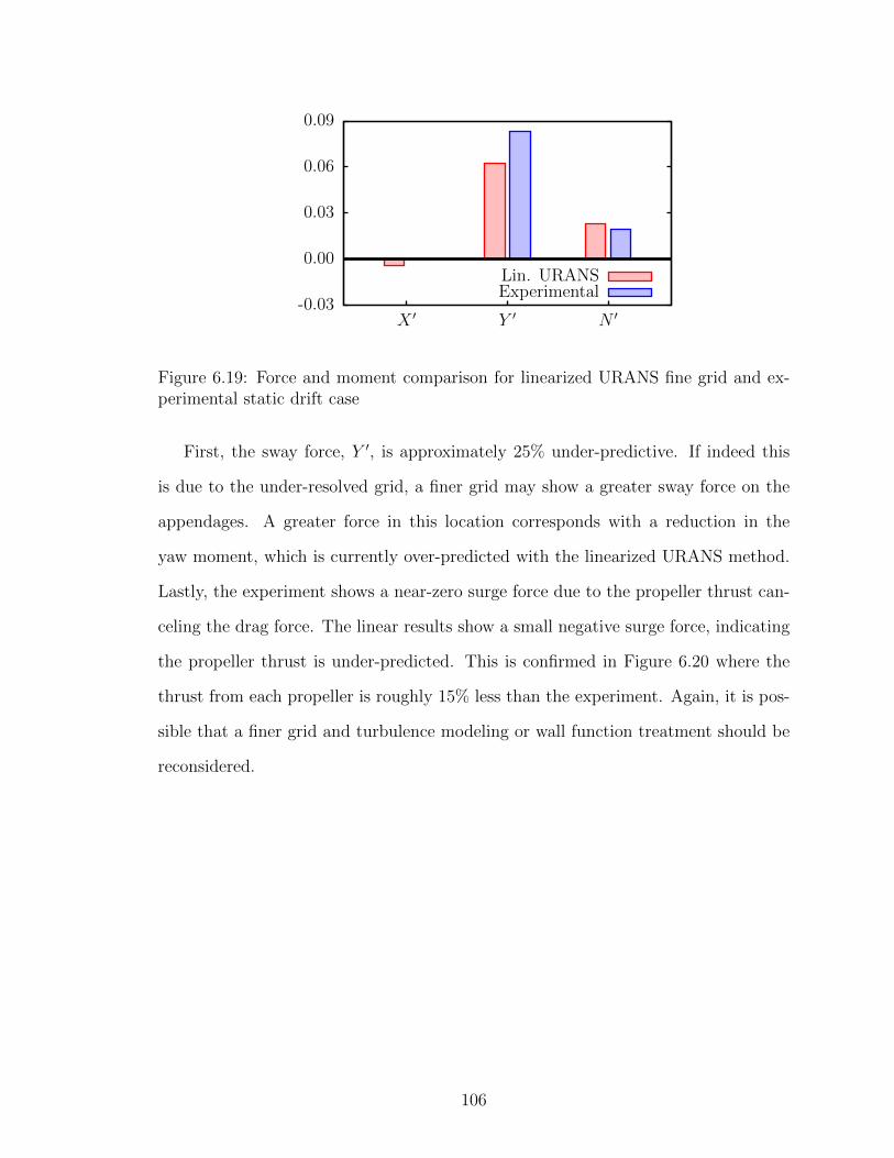
-0.03
0.00
0.03
0.06
0.09
X ′ Y ′ N ′
Lin. URANSExperimental
Figure 6.19: Force and moment comparison for linearized URANS fine grid and ex-perimental static drift case
First, the sway force, Y ′, is approximately 25% under-predictive. If indeed this
is due to the under-resolved grid, a finer grid may show a greater sway force on the
appendages. A greater force in this location corresponds with a reduction in the
yaw moment, which is currently over-predicted with the linearized URANS method.
Lastly, the experiment shows a near-zero surge force due to the propeller thrust can-
celing the drag force. The linear results show a small negative surge force, indicating
the propeller thrust is under-predicted. This is confirmed in Figure 6.20 where the
thrust from each propeller is roughly 15% less than the experiment. Again, it is pos-
sible that a finer grid and turbulence modeling or wall function treatment should be
reconsidered.
106

0.000
0.003
0.006
0.009
0.012
0.015
port stbd
T′
Lin. URANSExperimental
Figure 6.20: Propeller thrust from the fine grid during static drift compared to ex-perimental value
Adding the difference in numerical and experimental thrust force to the surge
force does result in a near-zero surge force, X ′ = 0.005. Nevertheless, the time series
from the port-side propeller in Figure 6.21 shows a steady state is achieved with a
time-averaged thrust, but there is a variation in force about this mean.
0.000
0.006
0.012
0.018
0.024
0 5 10 15 20 25 30 35 40
T′
t [s]
Lin. URANS
Figure 6.21: Propeller thrust during static drift over time
Closer inspection of the variation within the propeller thrust is displayed in Fig-
ure 6.22. Here, the impulses in the signal are seen to coincide with blade-passings.
The propellers have five blades, so five impulses per revolution are produced. The
angle of the A-frame bracket supporting the propeller shaft is such that blades simul-
taneously pass behind each leg of the bracket.
107

0.008
0.009
0.010
0.011
0.012
0.013
0.014
0 0.5 1 1.5 2
T′
Num. propeller rotations
Lin. URANS
Figure 6.22: Propeller thrust during static drift showing impulses due to blade-passings
Overall, the difficulties with modeling an actual propeller and obtaining an accu-
rate thrust suggest that alternatives such as a body force model may be a worthwhile
pursuit with the linearized URANS method.
108

CHAPTER VII
Conclusions and Future Work
7.1 Summary
A linearized free-surface URANS method is shown to be a promising approach
to accurately predicting ship maneuvering. The simplification of satisfying a first-
order wave condition gives rise to computational savings compared to fully nonlinear
methods, as there is far less of a need to resolve grids near the surface of the water.
Grid convergence is more readily achieved using many fewer cells than required with
fully nonlinear methods. The single-phase approach accounts for the viscous effects
which are of great importance in maneuvering, especially the interactions between the
hull, propellers, and rudders. Ship hulls with moving rudders and rotating propellers
may be simulated with fully rigid meshes in an inertial, Earth-fixed frame of reference.
A viscous air-water interface study has been performed in a two-dimensional man-
ner with a transom stern geometry. Typical flows produced in ship maneuvering are
replicated by varying the acceleration due to gravity, g, and the molecular viscosity, µ.
The range of transom-based Froude numbers tested (FrT = 3, FrT = 2, FrT = 0.3)
result in a steady wave, an unsteady breaking wave, and a nearly flat air-water inter-
face. A range of Reynolds numbers are also tested (Re = 1e4, Re = 1e5, Re = 1e6),
but this has far less of an effect on the flow. Viscous terms are shown to simply scale
linearly with the changes in molecular viscosity, µ. The findings from this study jus-
109

tify the use of linearized dynamic and kinematic free-surface boundary conditions in
conjunction with the RANS variables for ship maneuvering prediction. The suitabil-
ity of a linearized free-surface is further shown with a replication of the study using
the linearized URANS method. The wave elevations at each Froude number compare
well to those obtained with a fully nonlinear VOF method.
An initial test of the linearized URANS method in a ship-fixed reference frame
is applied to a KCS hull model performing forward speed tests at a range of Froude
numbers. The wave profile along the hull is compared against experiments, and the
agreement is quite good. Slight differences at the transom may be improved with the
use of the custom boundary condition for the free-surface elevation, imposed at the
free-surface/body juncture, which these simulations do not employ. In addition, the
sinkage and trim are calculated and shown to compare very well with the experimental
data.
A David Taylor Model Basin 5415 destroyer hull is extensive tested with a variety
of prescribed motion maneuvers. A bare hull version of the model, fitted only with
bilge keels, undergoes static drift, pure sway, and pure yaw maneuvers. For the static
drift simulations, the linearized URANS method is shown to require only a slight
increase in computational expense of 10% compared to a double-body approximation.
However, the linearized approach agrees with experimental data within 5% for the
surge force, sway force, and yaw moment. The double-body approximation differs
by over 20% for the sway force and yaw moment. The linearized URANS method
continues to agree closely with experimental predictions for the pure sway and pure
yaw maneuvers. Nonlinear simulations show little improvement in force predictions,
and at times less accurate results are displayed. The computational expense required
for the forces compared is up to 30 times less for the linearized URANS method than
a fully nonlinear level-set approach.
The appended version of the DTMB 5415 hull is analyzed with a static drift
110

maneuvering test. The five-bladed propellers operate at the design speed rotation
rate for each simulation. Results are not closely agreeable to the experimental data.
It is possible that greater resolution is required near the transom which contains many
appendages with complex geometries.
The results discussed in this thesis are an initial application and validation of the
technology, but they have shown the linearized URANS method to be a viable option
for ship designers compared to model tests and fully nonlinear CFD. Time and cost
savings allow for an increased number of hull forms to be evaluated, which in turn
provides a more complete exploration of a design space. Novel hull forms may be
better suited for their needs due to a more optimized geometry. There exists much
room for improvement with the linearized URANS method, but this only provides an
opportunity for naval architects to improve the designs of the largest moving objects
in the world.
7.2 Contributions
• It is demonstrated that the VOF method satisfies the air-water interface condi-
tion, with the stresses from the air and the water being small at the interface.
The small values of stress from the air demonstrate the suitability of the free-
surface assumption for ship maneuvering prediction. The terms within the total
stress vector of the water are evaluated to determine which terms to include in a
pressure boundary condition. For each case, it is shown that the viscous terms
are extremely small and may be neglected. Furthermore, the hydrodynamic and
hydrostatic pressures are shown to dominate. Therefore, assigning an inviscid,
zero total pressure condition at the z = 0 calm-water plane is justified for the
linearized URANS method.
• The linearized kinematic condition is shown to differ little from the nonlin-
111

ear condition and the actual condition from the solution of the transom stern
studies. This truly quantitative investigation has further justified the use of a
linearized kinematic condition for maneuvering simulations beyond the classical
linearization procedures.
• A URANS maneuvering prediction toolkit employing a linearized free-surface
has been developed. It is a single-phase finite-volume method built within the
OpenFOAM environment. Several unique features are implemented in a custom
fashion. A new pressure boundary condition coupled with a free-surface cell-
extrusion solves the linearized dynamic and kinematic free-surface boundary
conditions, respectively. These are solved in an inertial, Earth-fixed reference
frame. Multiple new mesh motion functions exist allowing for pure sway, pure
yaw, and free running model tests. Hulls with rotating propellers and moving
rudders are also possible, and gradual motion development over time is used
extensively in the new motion functions to aid in reducing problems associated
with impulsive starts.
7.3 Future Work
All results generated with the linearized URANS method presented in this thesis are
calculated with a maximum Courant number of just Cmax = 2. Stability issues arise
with Courant numbers greater than two. Although the exact cause is not known, it is
believed that this is from the implementation of the kinematic free-surface boundary
condition and is a problem which can be overcome. Fully nonlinear methods can
employ Courant numbers of Cmax = 50 for ship maneuvering problems. Therefore,
investigating the cause of this instability with the linearized URANS method presents
an opportunity to increase the computational efficiency of the method, possibly by
an order of magnitude.
112

An additional source of instability is found within the quality of grids which may
be used with the linearized URANS method. Grids which are seemingly suitable
for computations in terms of non-orthogonality, skewness, resolution, et cetera, can
result in diverging values of the free-surface elevation. This may be directly related
to the issues previously described with increasing the maximum allowable Courant
number. It may be possible that a unique investigation is required in order to deter-
mine the discretization requirements for applying the kinematic free-surface boundary
condition.
The custom boundary condition used at the intersection of the body and the
free-surface allows users to select an angle where the condition on the free-surface
elevation transitions from a zero normal-gradient condition to a mixed condition.
The angle is the difference between the body velocity and the body normal vector.
The boundary condition should be further developed to include a another angle at
which the condition becomes fixed-value. Currently, the condition only becomes fixed-
value when the vectors are aligned. Additional development could include a feature
which dynamically changes the boundary condition based on the magnitude of the
body velocity. In other words, a dynamically changing fixed-value. This may be
useful near the transom stern of an accelerating hull, where the free-surface elevation
is initially at the calm waterline but gradually decreases as the vessel increases speed.
The linearized URANS method is studied extensively with prescribed motion ma-
neuvers resembling those performed with PMMs. Rotating arm simulations are also
of concern to designers due to the rotary maneuvering coefficients that may be ob-
tained, and this is an area where the linearized URANS method could be further
tested. In addition, free-running model tests are possible, and these self-propelled
simulations are valuable for a number of reasons. They may provide knowledge of
propeller meshing requirements for accurate thrust prediction which is important for
achieving design speed in a self-propelled model test. Also, zig-zag and turning cir-
113

cle tests could indicate whether neglecting roll, heave, and pitch is still a suitable
approximation.
Results from LES simulations are provided in this thesis, but subsequent studies
may provide valuable insight about the extent to which the linearized free-surface
changes the fluid flow for ship maneuvering. The method may be suitable for studies
such as propeller inflow simulations while remaining less computationally burdensome
than fully nonlinear LES.
Lastly, waves could be added to the linearized URANS tool to provide predictions
for maneuvering in regular and irregular waves. The ability to perform these simula-
tions in an efficient manner is extremely important to designers. A goal to motivate
future work is to develop the capability to accurately and robustly perform full-scale,
self-propelled maneuvers in an irregular seaway.
114
APPENDIX
115
APPENDIX A
Viscous Interface Study – Unsteady Breaking
Wave
This appendix contains iso-surfaces from the unsteady breaking wave case in the
two-dimensional transom stern canonical study. The transom-based Froude number
is FrT = 2. Results are shown for Reynolds numbers of Re = 1e5 and Re = 1e6.
A discussion of the results corresponding to Re = 1e4 appears in Chapter V. Four
iso-surfaces are associated with each Reynolds number. First, two figures are used to
display the dimensionless viscous stresses from the total stress vector. One is from the
horizontal component of the of the vector and the other from the vertical component,
in this form respectively:
| 2µeffuxq | + | µeff (uz + wx) s |12ρU2
(A.1)
| µeff (wx + uz) q | + | 2µeffwzs |12ρU2
(A.2)
The main conclusion from the investigation of the viscous stresses is that they are
very small at the surface of the water. Additionally, the viscous terms scale linearly
with changes in Reynolds number within the studied range (Re = 1e5 − 1e6). The
116
small magnitude of these terms suggests that they may be neglected when seeking
appropriate boundary conditions for a free-surface approximation. Next, two figures
are used to display the dimensionless hydrodynamic and hydrostatic pressures from
the vertical component of the stress vector:
ps12ρU2
(A.3)
ρgηs12ρU2
(A.4)
The most important observation from the hydrostatic and hydrodynamic pressure
is that they are much greater than the viscous stresses at the surface of the water.
They are the most influential terms when considering a suitable pressure boundary
condition to apply with a free-surface approximation. Also, the iso-surface from the
static pressure and dynamic pressure are nearly identical, indicating that they are in
balance. Thus, collecting the dominant terms from the total stress vector results in
a single, inviscid total pressure condition in the vertical direction:
p− ρgη = 0 (A.5)
This is the boundary condition used for the dynamic pressure at the free-surface of
the linearized URANS method.
117

t = 0
t = 1 s
t = 2 s
t = 3 s
0 5e-06
t = 4 s
| 2µeffuxq | + | µeff (uz + wx) s |12ρU2
Figure A.1: Re=1e5, Magnitudes of the horizontal viscous stresses as the wave breaks
118
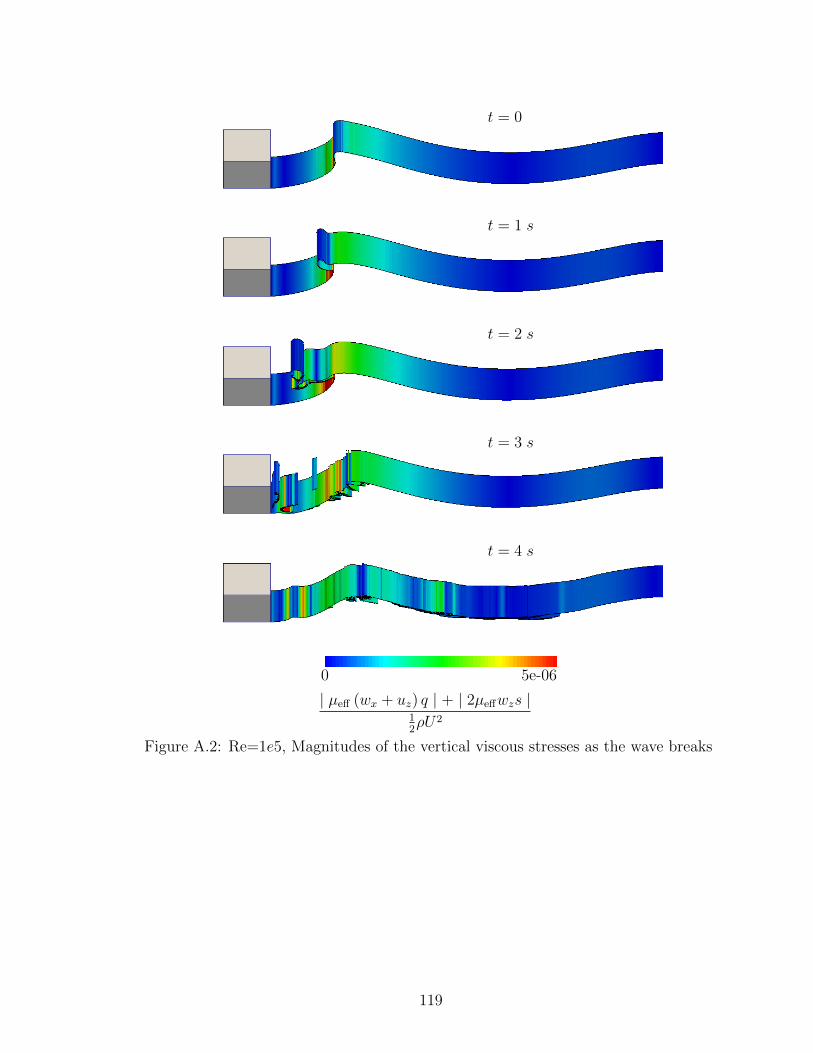
t = 0
t = 1 s
t = 2 s
t = 3 s
0 5e-06
t = 4 s
| µeff (wx + uz) q | + | 2µeffwzs |12ρU2
Figure A.2: Re=1e5, Magnitudes of the vertical viscous stresses as the wave breaks
119
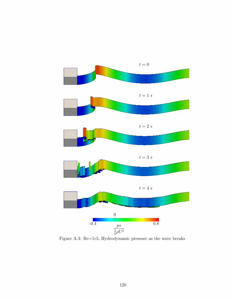
t = 0
t = 1 s
t = 2 s
t = 3 s
0
-0.4 0.8
t = 4 s
ps12ρU2
Figure A.3: Re=1e5, Hydrodynamic pressure as the wave breaks
120
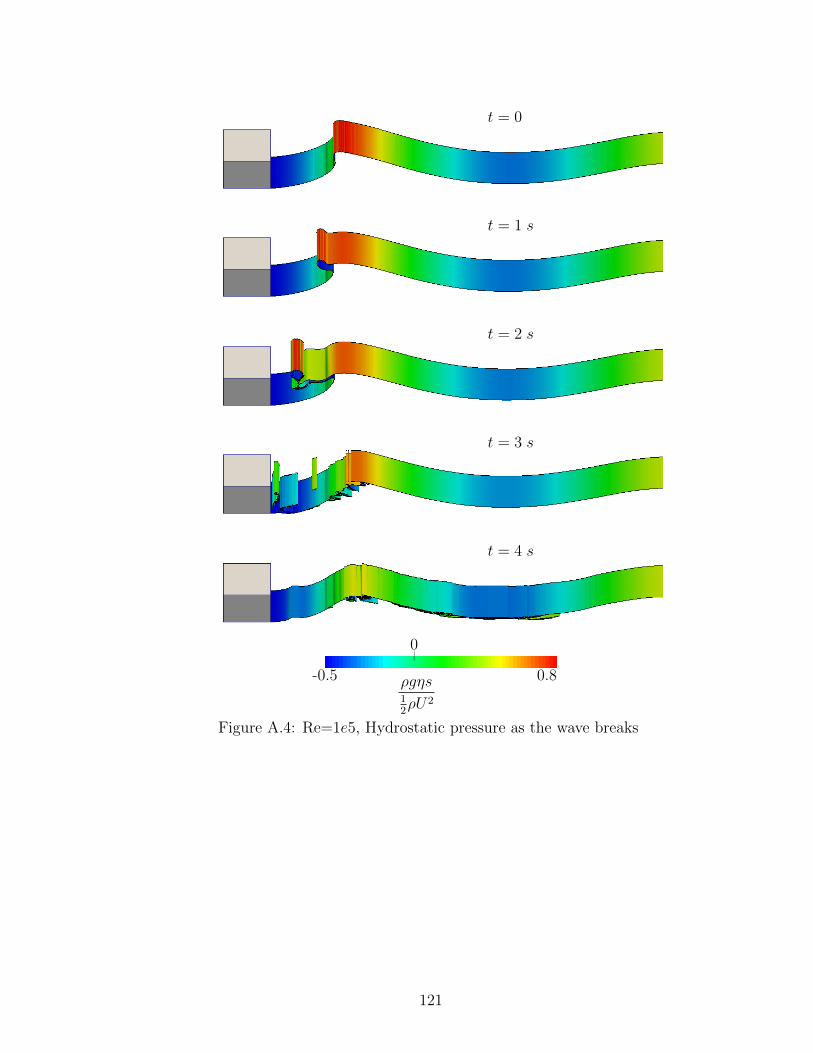
t = 0
t = 1 s
t = 2 s
t = 3 s
0
-0.5 0.8
t = 4 s
ρgηs12ρU2
Figure A.4: Re=1e5, Hydrostatic pressure as the wave breaks
121

t = 0
t = 1 s
t = 2 s
t = 3 s
0 5e-07
t = 4 s
| 2µeffuxq | + | µeff (uz + wx) s |12ρU2
Figure A.5: Re=1e6, Magnitudes of horizontal viscous stresses as the wave breaks
122

t = 0
t = 1 s
t = 2 s
t = 3 s
0 5e-07
t = 4 s
| µeff (wx + uz) q | + | 2µeffwzs |12ρU2
Figure A.6: Re=1e6, Magnitudes of vertical viscous stresses as the wave breaks
123
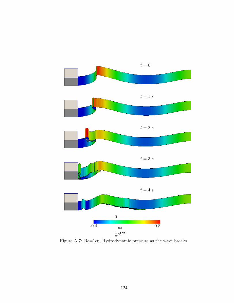
t = 0
t = 1 s
t = 2 s
t = 3 s
0
-0.4 0.8
t = 4 s
ps12ρU2
Figure A.7: Re=1e6, Hydrodynamic pressure as the wave breaks
124
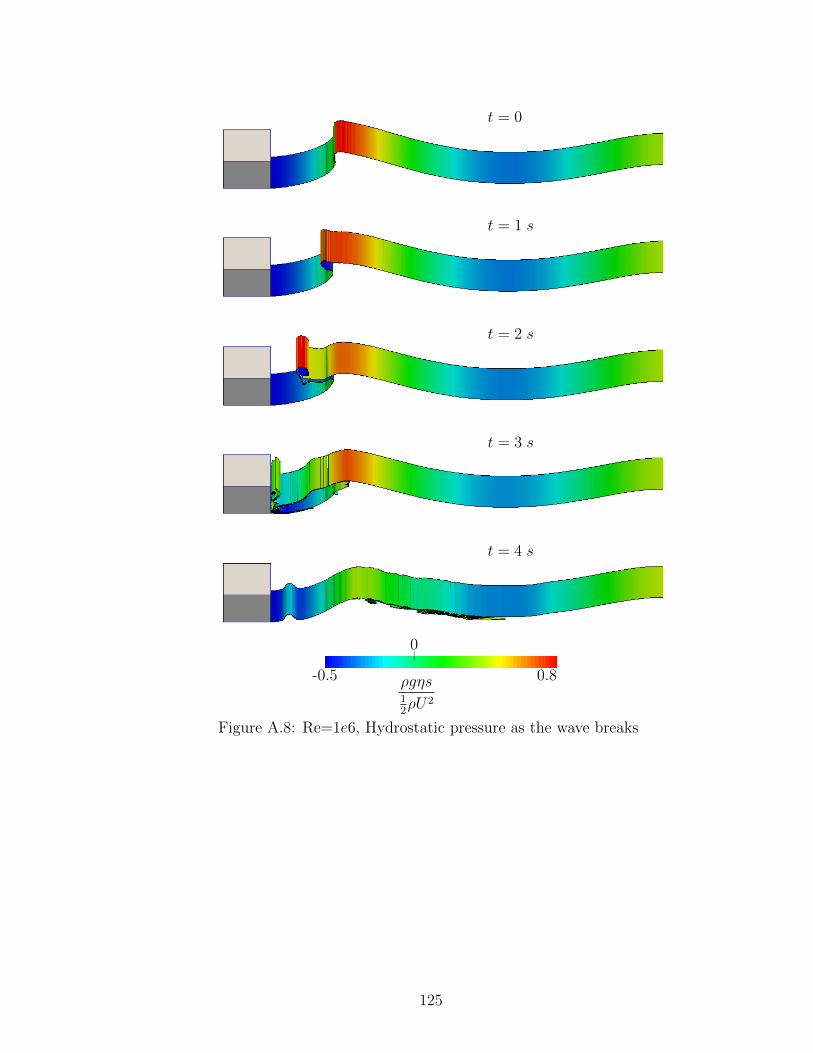
t = 0
t = 1 s
t = 2 s
t = 3 s
0
-0.5 0.8
t = 4 s
ρgηs12ρU2
Figure A.8: Re=1e6, Hydrostatic pressure as the wave breaks
125

BIBLIOGRAPHY
126

BIBLIOGRAPHY
ABS. Guide for vessel maneuverability, March 2006.
Agdrup, K. Model test report. Technical report, FORCE Technology, Denmark, 2004.
Araki, M., Ohashi, K., and Hirata, N. KVLCC2 simulations with overset grid method.In Otzen and Simonsen (2014).
ASME. Procedure for estimation and reporting of uncertainty due to discretizationin CFD applications, 2008.
Barton, I. E. Comparison of SIMPLE- and PISO-type algorithms for transient flows.International Journal For Numerical Methods In Fluids, 26:459–483, 1998.
Beck, R. F. and Loken, A. E. Three-dimensional effects in ship relative-motion prob-lems. Journal of Ship Research, 33:261–268, 1989.
Beck, R. F., Newman, J. N., and Tuck, E. D. Hydrodynamic forces on ships indredged channels. Journal of Ship Research, 19, 1975.
Belenky, V. and Falzarano, J. Rating-based maneuverability standards. Technicalreport, American Bureau of Shipping, 2006.
Broglia, R., Muscari, R., and Mascio, A. D. Numerical simulations of the pure swayand pure yaw motion of the kvlcc-1 and 2 tankers. In Stern and Agdrup (2008).
Broglia, R., Dubbioso, G., Durante, D., and Di Mascio, A. Simulation of turning circleby CFD: Analysis of different propeller models and their effect on manoeuvringprediction. Applied Ocean Research, 39:1–10, 2013.
Burg, C. O. E. and Marcum, D. L. Moving towards high-fidelity RANS calcula-tions of maneuvering surface vessels using unstructured grids. In 8th InternationalConference on Numerical Ship Hydrodynamics, 2003.
Carrica, P. M., Ismail, F., Hyman, M., Bhushan, S., and Stern, F. Turn and zigzagmaneuvers of a surface combatant using a URANS approach with dynamic oversetgrids. Journal of Marine Science and Technology, 18(2):166–181, 2012.
Cope, D. M. Design of a free-running 1/30th Froude scaled model destroyer for in-situ hydrodynamic flow visualization. Master’s thesis, Massachusetts Institute ofTechnology, 2012.
127
de Boer, J. Model making to the tune of 150 a year. Technical report, MARIN, 2009.
Eca, L. Discretization uncertainty estimation based on a least squares version of thegrid convergence index. October 2006.
Farrell, P. and Maddison, J. Conservative interpolation between volume meshes bylocal Galerkin projection. Computational Methods in Applied Mechanics and En-gineering, 200:89–100, 2011.
Filip, G. P. High-Resolution Numerical Simulation of Turbulent Interfacial MarineFlows. PhD thesis, University of Michigan, 2013.
Furukawa, Y., Nakiri, Y., Kijima, K., and Ibaragi, H. The prediction of the manoeu-vrability of KVLCC1 and KVLCC2. In Stern and Agdrup (2008).
Gillespie, J. W. A Network Science Approach to Understanding and Generating ShipArrangements in Early-Stage Design. PhD thesis, University of Michigan, 2012.
Hallmann, R. Applicability rotating arm: validation and extension of the rotating armfunctionality in the seakeeping and manoeuvring basin. Technical report, MARIN,2007.
Havelock, T. H. The resistance of a ship among waves. In Proceedings of the RoyalSociety of London, volume 161 of Series A, Mathematical and Physical Sciences,pages 299–308. The Royal Society, August 1937.
Havelock, T. H. The pressure of water waves upon a fixed obstacle. In Proceedings ofthe Royal Society of London, volume 175 of Series A, Mathematical and PhysicalSciences, pages 409–421. The Royal Society, July 1940.
Hirt, C. W. and Nichols, B. D. Volume of fluid (VOF) method for the dynamics offree boundaries. Journal of Computational Physics, 39:201–225, 1981.
Hochbaum, A. C., Vogt, M., and Gatchell, S. Manoeuvering prediction for two tankersbased on RANS simulations. In Stern and Agdrup (2008).
Holtrop, J. and Mennen, G. G. J. A statistical power prediction method. InternationalShipbuilding Progress, 25:253–256, 1978.
Holtrop, J. and Mennen, G. G. J. An approximate power prediction method. Inter-national Shipbuilding Progress, 29:166–170, 1982.
Hong, W. and Walker, D. T. Reynolds-averaged equations for free-surface flows withapplication to high-Froude-number jet spreading. J. Fluid Mech., 417:183–209,2000.
IMO. Explanatory notes to the standards for ship manoeuvrability, 2002.
Issa, R. J. Solutions of the implicitly discretised fluid flow equations by operator-splitting. Journal of Computational Physics, 1986.
128

ITTC. Recommended procedures - testing and extrapolation methods: Manoeuvra-bility: Free-sailing model test procedure, 2002.
Jasak, H. Error Analysis and Estimation for the Finite Volume Method with Appli-cations to Fluid Flows. PhD thesis, Imperial College, University of London, 1996.
Kelvin, B. On ship waves. In Institution of Mechanical Engineers. Institution ofMechanical Engineers, 1887.
Kim, K. Simulation of surface ship dynamics using unsteady RANS codes. Technicalreport, Office of Naval Research, 2002.
Kim, S. Y. and Kim, Y. G. Prediction of maneuvering performance for KVLCC1 andKVLCC2 based on PMM data. In Stern and Agdrup (2008).
Kring, D. C., Parish, M. K., Milewski, W. M., and Connell, B. S. H. Simulation ofmaneuvering in waves for a high-speed surface effect ship. In 11th InternationalConference on Fast Sea Transportation. Navatek, Ltd, September 2011.
Lafaurie, B., Nardone, C., Scardovelli, R., Zaleski, S., and Zanetti, G. Modelingmerging and fragmentation in multiphase flows with SURFER. Journal of Com-putational Physics, 113:134–147, 1994.
Lincoln, C. C., Eda, H., and Landsburg, A. C. Principles of Naval Architecture:Volume III - Motions in Waves and Controllability. The Society of Naval Architectsand Marine Engineers, 1989.
Longo, J., Yoon, H.-S., Toda, Y., and Stern, F. Phase-averaged 3DPIV/wave eleva-tions and force/moment measurements for surface compatant in PMM maneuvers.In Proc. 26th ONR Symposium on Naval Hydrodynamics, Rome, Italy, 2006.
Maki, K. J. Transom Stern Hydrodynamics. PhD thesis, University of Michigan,2006.
Maki, K. J. and Wilson, W. M. Steady drift force calculation on the naval destroyerhull 5415. In Stern and Agdrup (2008).
McNaughton, J., Afgan, I., Apsley, D. D., Rolfo, S., Stallard, T., and Stansby, P. K. Asimple sliding-mesh interface procedure and its application to the CFD suimulationof a tidal-stream turbine. International Journal For Numerical Methods In Fluids,74:250–269, 2014.
Miller, R. W. PMM calculations for the bare and appended DTMB 5415 using theRANS solver CFDSHIP-IOWA. In Stern and Agdrup (2008).
Newman, J. N. and Tuck, E. O. Hydrodynamic interaction between two ships. InProceedings of the 10th Symposium on Naval Hydrodynamics, pages 35–70, 1974.
Noblesse, F. and Yang, C. Elementary water waves. Journal of Engineering Mathe-matics, 59:277–299, 2007.
129

Noblesse, F., Delhommeau, G., Huang, F., and Yang, C. Practical mathematicalrepresentation of the flow due toa distribution of sources on a steadily advancingship hull. Journal of Engineering Mathematics, 71:367–392, 2011.
Noblesse, F., Huang, F., and Yang, C. The Neumann-Kelvin theory of ship waves.Journal of Engineering Mathematics, 79:1–20, 2013.
Otzen, J. F. and Simonsen, C. D., editors. Proceedings SIMMAN 2014 Workshop,Copenhagen, Denmark, December 2014.
Parsons, M. G., Chung, H., Nick, E., Daniels, A., Liu, S., and Patel, J. Intelligent shiparrangements: A new approach to general arrangement. Naval Engineers Journal,120:51–65, 2008.
Pivano, L. Thrust Estimation and Control of Marine Propellers in Four-QuadrantOperations. PhD thesis, Norwegian University of Science and Technology, April2008.
Rood, E. P. Fluid Vortices, volume 30. Springer Netherlands, 1995.
Rosemurgy, W. J., Edmund, D. O., Maki, K. J., and Beck, R. F. A velocity de-compostion approach for steady free-surface flow. In 29th Symposium on NavalHydrodynamics. The National Academies Press, August 2012.
Salvesen, N., Tuck, E. D., and Faltinson, O. Ship motions and sea loads. In TheSociecty of Naval Architects and Marine Engineers, 1970.
Sclavounos, P. D. and Thomas, B. S. Optimal control theory applied to ship ma-neuvering in restricted waters. Journal of Engineering Mathematics, 58:301–315,2007.
Shen, L., Zhang, X., Yue, D. K. P., and Triantafyllou, G. S. The surface layer forfree-surface turbulent flows. J. Fluid Mech., 386:167–212, 1999.
Shen, L., Triantafyllou, G. S., and Yue, D. K. P. Turbulent diffusion near a freesurface. J. Fluid Mech., 407:145–166, 2000.
Shen, L., Zhang, C., and Yue, D. K. P. Free-surface turbulent wake behind towedship models: experimental measurements, stability, analyses and direct numericalsimulations. J. Fluid Mech., 469:89–120, 2002.
Shen, Z., Wan, D., and Carrica, P. M. RANS simulations of free maneuvers withmoving rudders and propellers using overset grids in OpenFOAM. In Otzen andSimonsen (2014).
Simonsen, C. D., Otzen, J. F., Klimt, C., Larsen, N. L., and Stern, F. Maneuveringpredictions in the early design phase using CFD generated PMM data. In 29thSymposium on Naval Hydrodynamics, August 2012.
130
Singer, D. J., Doerry, N., and Buckley, M. E. What is set-based design? NavalEngineers Journal, 121:31–43, 2009.
Soding, H. Limits of potential theory in rudder flow predictions. In 22nd Sym-posium on Naval Hydrodynamics. The National Academies Press, 1999. ISBN9780309065375.
Spalart, P. R. and Allmaras, S. R. A one-equation turbulence model for aerodynamicflows. In AIAA Meeting 92-0439, January 1992.
Stern, F. and Agdrup, K., editors. Proceedings SIMMAN 2008 Workshop, Copen-hagen, Denmark, 2008.
Strock, J. and Brown, A. Methods for naval ship concept and propulsion technologyexploration in a CGX case study. Naval Engineers Journal, 120:95–122, 2008.
Tanizawa, K. and Naito, S. An application of fully nonlinear numerical wave tankto the study on chaotic roll motions. In Chung, J. S., Matsui, T., Naito, S., andSayed, M., editors, Proceedings of the Eighth (1998) International Offshore andPolar Engineering Conference, volume 3, pages 280–287. International Society ofOffshore and Polar Engineers, May 1998.
Toxopeus, S. L. Deriving mathematical manoeuvring models for bare ship hulls usingviscous flow calculations. Journal of Marine Science and Technology, 14:30–38,2009.
Turnock, S. R., Phillips, A. B., and Furlong, M. URANS simulations of static driftand dynamic manouveres of the KVLCC2 tanker. In Stern and Agdrup (2008).
Ueno, M., Tsukada, Y., and Kitagawa, Y. Rudder effectiveness correction for scalemodel ship testing. Ocean Engineering, 92:267 – 284, 2014.
van Brummelen, H. Numerical Methods for Steady Viscous Free-Surface Flows. PhDthesis, University of Amsterdam, 2002.
Vukcevic, V., Ostman, A., and Jasak, H. Rapid simulations of pure sway motionusing FVM in OpenFOAM. In Otzen and Simonsen (2014).
Wang, H., Tian, X., Zou, Z., and B., W. Experimental and numerical researches onthe viscous hydrodynamic forces acting on a KVLCC2 model in oblique motion. InStern and Agdrup (2008).
Yeh, H. Advances in Coastal and Ocean Engineering. World Scientific Publishing,1995.
131