a little aspect of real analysis, topology and probability
TRANSCRIPT

Governors State UniversityOPUS Open Portal to University Scholarship
All Student Theses Student Theses
Summer 2016
A Little Aspect of Real Analysis, Topology andProbabilityAsmaa A. AbdulhameedGovernors State University
Follow this and additional works at: http://opus.govst.edu/theses
Part of the Mathematics Commons
For more information about the academic degree, extended learning, and certificate programs of Governors State University, go tohttp://www.govst.edu/Academics/Degree_Programs_and_Certifications/
Visit the Governors State Mathematics DepartmentThis Thesis is brought to you for free and open access by the Student Theses at OPUS Open Portal to University Scholarship. It has been accepted forinclusion in All Student Theses by an authorized administrator of OPUS Open Portal to University Scholarship. For more information, please [email protected].
Recommended CitationAbdulhameed, Asmaa A., "A Little Aspect of Real Analysis, Topology and Probability" (2016). All Student Theses. Paper 81.

A LITTLE ASPECT OF REAL ANALYSIS, TOPOLOGY AND
PROBABILITY
By
Asmaa A. Abdulhameed
B.A., Trinity Christian College, 2012
Thesis
Submitted in partial fulfillment of the requirements
For the Degree of Master of Science, With a Major in Mathematics
Governors State University University Park, IL 60484
2016

2
Table of Contents ABSTRACT .................................................................................................................................... 5
INTRODUCTION .......................................................................................................................... 6
PART ONE : MERTIC, NORMED VECTOR SPACE AND TOPOLOGICAL SPACES ........... 7
1. Metric Space (Distance Function) 𝑋𝑋,𝑑𝑑 ....................................................................................... 7
2. Norms and Normed Vector Spaces (V,‖ ∙‖) ............................................................................... 8
2.1 Different Kinds of Norms ......................................................................................................... 9
2.2 Ball in ℓ𝑝𝑝 ................................................................................................................................. 10
2.3 𝐿𝐿𝑝𝑝 Space (Function Spaces) .................................................................................................... 10
2.4 Distance Between Functions, 𝐿𝐿𝑝𝑝-distance ............................................................................. 11
3. Topological space ..................................................................................................................... 12
3.1 Continuous Function in Metric and Topology ........................................................................ 13
3.2 Limit Point .............................................................................................................................. 15
PART TWO : OUTLINES OF MEASURE AND PROBABILITY SPACES............................. 16
1. Measure and Measure Space ..................................................................................................... 16
1.1 Construction of Sigma Algebra 𝜎𝜎(𝒜𝒜) .................................................................................... 17
1.2 The Inverse Function is Measurable Function ........................................................................ 18
2. Probability Space ...................................................................................................................... 20
2.1 Sample Space Ω ...................................................................................................................... 21
2.2 The 𝜎𝜎-field and Class of Events ℱ .......................................................................................... 21
2.3 Sequences of Events in Probability......................................................................................... 22
2.4 Continuity Theorems of Probability ....................................................................................... 23
3. General Idea of Borel Set .......................................................................................................... 23
3.1 Complicated Borel Sets (Cantor set)....................................................................................... 25
3.2 Borel 𝜎𝜎-algebra in Topology ................................................................................................ 26
3.3 Borel Set of Probability Space ................................................................................................ 27
4. Measurable Space in Probability ............................................................................................. 27
5. Random Variable (R.V) ............................................................................................................ 28
5.1 Measurable Function is a Random Variable ........................................................................... 29
PART THREE: MEASURE AND PROBABILITY THEORY AND DISTRIBUTION FUNCTION .................................................................................................................................. 31
1. Lebesgue’s Idea of Integral (subdivide the range) .................................................................... 31
2. Additive Set Function and Countable Additivity...................................................................... 33
3. Construction of Measure on ℝ, ℝ2 and ℝ3............................................................................... 34

3
4. Hyper Rectangles and Hyperplanes {𝐻𝐻𝐻𝐻} .................................................................................. 35
5. Lebesgue Measures on ℝ and ℝ𝑛𝑛 ............................................................................................. 37
6. Basic Definitions and Properties ............................................................................................... 39
6.1 Measure Extension from Ring To 𝜎𝜎-ring................................................................................ 40
7. The Outer Measure ................................................................................................................... 40
7.1 Premeasure .............................................................................................................................. 43
7.2 Extending the Measure by Carathedory’s Theorem ............................................................... 43
8. Lebesgue, Uniform Measure on [0,1] and Borel Line .............................................................. 45
9. The Advantage of Measurable Function ................................................................................... 46
10. Induced Measure ..................................................................................................................... 47
11. Probability Space and the Distribution Function .................................................................... 49
12. Lebesgue-Stieltjes Measure .................................................................................................... 51
12.1 Lebesgue-Stieltjes Measure as a Model for Distributions .................................................... 52
13. Properties of the Distribution Function................................................................................... 52
14. Relate the Measure 𝜇𝜇 to the Distribution Function, 𝐹𝐹 ............................................................ 54
15. Distribution Function onℝ𝑛𝑛 .................................................................................................... 54
CONCLUSION IN GENERAL .................................................................................................... 59
REFERENCES ............................................................................................................................. 60

4
List of Figures
Figure 1 Metric spaces and topology space ....................................................................................7 Figure 2 Diagram of triangle equality in metric space ....................................................................7 Figure 3 Ball inℝ2 with the ℓ1, ℓ2, ℓ∞ norms .....................................................................................10 Figure 4 The convergence of the sequence ................................................................................... 14 Figure 5 Measure on a set, S ..........................................................................................................16 Figure 6 Constructing sigma algebra ..................................................................................................18 Figure 7 mapping 𝑓𝑓:𝑋𝑋 ⟶ 𝑌𝑌 ..........................................................................................................19 Figure 8 𝑓𝑓 is measurable function because of 𝑓𝑓−1 exist ...............................................................19 Figure 9 A probability measure mapping the probability space ....................................................20 Figure 10 Borel set .........................................................................................................................26 Figure 11 Borel sets, 𝐸𝐸 is a collection of subsets of Ω .................................................................26 Figure 12 Two measurable spaces .................................................................................................28 Figure 13 The transformation of some sample points ..................................................................29 Figure 14. Example about Lebesgue integral ................................................................................32 Figure 15 two dimensional rectangle of half open intervals (𝑎𝑎1,𝑏𝑏1] × (𝑎𝑎2,𝑏𝑏2] .........................36 Figure 16 Lebesgue outer measure ................................................................................................41 Figure 17 Set ℳ ⊆ ℝ, left half open intervals covering ℳ .........................................................42 Figure 18 ℙ𝑓𝑓 is a probability measure on (ℝ,ℬ) ..........................................................................49 Figure 19 Cartesian product of 𝜇𝜇�(𝑎𝑎1,𝑏𝑏1] × (𝑎𝑎2,𝑏𝑏2]) ..................................................................56 Figure 20 Non Example .................................................................................................................56 Figure 21 Solution for Non Example .............................................................................................57
List of Tables
Table 1 interpretation of measure theory and probability theory concepts .............................................6 Table 2 Different Kind of vector norms are summarized ................................................................9 Table 3. Terminology of measure theory .......................................................................................18 Table 4. Terminology of set theory and probability theory ...........................................................21 Table 5 The relationship between premeasure, outer measure and measure ................................43 Table.6 Terminology for both measure space and the equivalent probability space ....................49

5
ABSTRACT
The body of the paper is divided into three parts:
Part one: include definitions and examples of the metric, norm and topology along with some
important terms such as metrics ℓ1, ℓ2, ℓ∞ and vector norm |𝑥𝑥|𝑝𝑝 which also known as the 𝐿𝐿𝑝𝑝
space. In case of the topology space this concept adjusted to be a unit ball that is distance one
from a point unit circle.
Part two: demonstrate the measure and probability which is one of the main topics in this work.
This section serves as an introduction for the remaining part. It explains the construction of the
𝜎𝜎-algebra and the Borel set, and the usefulness of the Borel set in the probability theory.
Part Three: to understand the measure, one has to understand finitely additive measure and
countable additivity of subsets, besides knowing the definition of ring, 𝜎𝜎-ring and their measure
extension. One also has to differentiate between the terms premeasure, outer measure and
measure from their domains and additivity conditions, which is clarified in the form of table.
The advantage of measurable function and the induced measure is explained, as both share to
define the probability as a measure, the probability that has values in the Borel set. As a
summary of this section, a Borel 𝜎𝜎-algebra shows a special role in real-life probability because
numerical data, real numbers, is gathered whenever a random experiment is performed.
In this work a simple technique that is supported by pictorial presentation mostly is used, and for
easiness most proofs are replaced by examples. I have freely borrowed a lot of material from
various sources, and collected them in the manner that makes this thesis equipped with a little
aspect of the real analysis, topology and probability theory.

6
INTRODUCTION
Probability space has its own vocabulary, which is inherited from probability theory. In modern
real analysis instead of the word set, the word space used, the word space is used to title a set that
has been endowed with a special structure. We therefore begin by presenting a brief list of real
analysis, probability and topological space dialect.
Analysts' Term Probabilists' Term Topological Term
Normed Measure space (𝑋𝑋,ℳ, 𝜇𝜇) Probability space (𝛺𝛺,ℱ,ℙ) or
called field of probability
Topological Space (𝑋𝑋,𝒯𝒯)
𝜎𝜎-algebras 𝜎𝜎(𝒜𝒜) and Borel set
𝒜𝒜: subset
𝜎𝜎-field 𝜎𝜎(𝐸𝐸) and Borel set
𝐸𝐸: Event
𝜎𝜎(𝒯𝒯) and Borel 𝜎𝜎-algebras
The Borel subsets of ℝ𝑛𝑛 is
the σ-algebra generated by
the open sets of ℝ𝑛𝑛 (with a
compact metric space)
Measurable function 𝑓𝑓
Measurable function (Random
variable)
Measurable space
Points in space Outcome, 𝜔𝜔 Points in space
Convergence in measure Convergence in probability Convergence in 𝜀𝜀-ball
the induced Measure 𝜇𝜇𝐹𝐹 (Lebesgue-
Stieltjes measure)
the induced Measure 𝜇𝜇𝐹𝐹
(Distribution)
Support Measure Theory (Lebesgue-Stieltjes measure)
Continuous function is measurable Measure induced by continuous random variable
Continuous function is
measurable
Table 1 Interpretation of measure theory and probability theory concepts (adopted from: Gerald B.
Folland, 1999).

7
PART ONE : MERTIC, NORMED VECTOR SPACE AND TOPOLOGICAL SPACES
Figure 1 Metric space topological space, but not all topological spaces can be metric
1. Metric Space (Distance Function) (𝑿𝑿,𝒅𝒅)
A metric space as a pair (𝑋𝑋,𝑑𝑑), where 𝑋𝑋 is a set and 𝑑𝑑 is a function that assign a real number
𝑑𝑑(𝑥𝑥,𝑦𝑦) to every pair 𝑥𝑥,𝑦𝑦 ∈ 𝑋𝑋 written as; 𝑑𝑑:𝑋𝑋 × 𝑋𝑋 ⟶ ℝ, and the Cartesian product 𝑋𝑋 × 𝑋𝑋 =
{ (𝑥𝑥, 𝑦𝑦)| 𝑥𝑥 ∈ 𝑋𝑋 𝑎𝑎𝑎𝑎𝑑𝑑 𝑦𝑦 ∈ 𝑋𝑋 }.
The distance function is 𝑑𝑑(𝑥𝑥,𝑦𝑦) and 𝑑𝑑 map the 𝑥𝑥 and 𝑦𝑦 to positive real number [0,∞) such that:
1. 𝑑𝑑(𝑥𝑥,𝑦𝑦) ≥ 0 for all 𝑥𝑥,𝑦𝑦 ∈ 𝑋𝑋 and 𝑑𝑑(𝑥𝑥,𝑦𝑦) = 0 if and only if 𝑥𝑥 = 𝑦𝑦,
2. 𝑑𝑑(𝑥𝑥,𝑦𝑦) = 𝑑𝑑(𝑦𝑦, 𝑥𝑥) for all 𝑥𝑥,𝑦𝑦 ∈ 𝑋𝑋;
3. 𝑑𝑑(𝑥𝑥, 𝑧𝑧) ≤ 𝑑𝑑(𝑥𝑥,𝑦𝑦) + 𝑑𝑑(𝑦𝑦, 𝑧𝑧) for all 𝑥𝑥,𝑦𝑦, 𝑧𝑧 ∈ 𝑋𝑋.
Condition (3) is called the triangle inequality because (when applied to ℝ2 with the usual metric)
it says that the sum of two sides of the triangle is at least as big as the third side(𝑎𝑎 + 𝑏𝑏 ≥ 𝑐𝑐).
Figure 2 Diagram of triangle equality in metric space (source: Ji�̆�𝑟i Lebl, 2011)

8
The plane ℝ2 with usual metric 𝑑𝑑1 is obtained from the measure of the horizontal and vertical
distance, and add the two together. 𝑑𝑑1�(𝑥𝑥1,𝑦𝑦1), (𝑥𝑥2,𝑦𝑦2)� = |𝑥𝑥1 − 𝑥𝑥2| + |𝑦𝑦1 − 𝑦𝑦2|.
The metric 𝑑𝑑2 obtained from Pythagoras’s theorem (called the Euclidean metric). For 𝑎𝑎 = 2, it
is defined by 𝑑𝑑2(𝑥𝑥, 𝑦𝑦) = �((𝑥𝑥1 − 𝑦𝑦1)2 + (𝑥𝑥2 − 𝑦𝑦2)2), where 𝑥𝑥 = (𝑥𝑥1, 𝑥𝑥2), 𝑦𝑦 = (𝑦𝑦1,𝑦𝑦2). For
𝑎𝑎 > 2, 𝑑𝑑2(𝑥𝑥,𝑦𝑦) = �((𝑥𝑥1 − 𝑦𝑦1)2 + (𝑥𝑥2 − 𝑦𝑦2)2 + ⋯ (𝑥𝑥𝑛𝑛 − 𝑦𝑦𝑛𝑛)2), where 𝑥𝑥 = (𝑥𝑥1, 𝑥𝑥2, … , 𝑥𝑥𝑛𝑛),𝑦𝑦 =
(𝑦𝑦1,𝑦𝑦2, … ,𝑦𝑦2).
The plane ℝ2 with the supremum metric 𝑑𝑑∞. 𝑑𝑑∞�(𝑥𝑥1,𝑦𝑦1), (𝑥𝑥2, 𝑦𝑦2)� = 𝑚𝑚𝑎𝑎𝑥𝑥 {|𝑥𝑥1 − 𝑥𝑥2|, |𝑦𝑦1 −
𝑦𝑦2|}. We can represent it as 𝑑𝑑∞:ℝ2 × ℝ2 → ℝ.
Note. Some reference use the notation ℓ1, ℓ2, ℓ∞ instead of d1 , d2 and d∞.
2. Norms and Normed Vector Spaces (V, ‖∙‖)
The norm is best thought of as a length, defined for functions in space, where it must satisfy
some properties. In linear algebra, we define a vector �⃗�𝑥 as an ordered tuple of numbers �⃗�𝑥 =
(𝑥𝑥1, 𝑥𝑥2, … , 𝑥𝑥𝑛𝑛). If 𝑋𝑋 is a vector space over ℝ, a norm is a function ‖∙‖:𝑋𝑋 → [0,∞) having the
following properties:
N1 ‖𝑥𝑥‖ > 0 when 𝑥𝑥 ≠ 0 and ‖𝑥𝑥‖ = 0 if and only if 𝑥𝑥 = 0.
N2 ‖𝛼𝛼𝑥𝑥‖= | 𝛼𝛼 | ・‖𝑥𝑥‖ for all 𝑥𝑥 ∈ 𝑋𝑋 and 𝛼𝛼 ∈ℝ, 𝛼𝛼 a scalar.
N3 ‖𝑥𝑥 + 𝑦𝑦‖ ≤‖𝑥𝑥‖ + ‖𝑦𝑦‖ for all 𝑥𝑥, 𝑦𝑦 ∈ 𝑋𝑋.
Note. A general vector norm |𝑥𝑥|, sometimes written with a double bar ‖𝑥𝑥‖ as above, is a
nonnegative norm.
The distance between two numbers 𝑥𝑥1 and 𝑥𝑥2 in ℝ is the absolute value of their difference is
𝑑𝑑(𝑥𝑥1, 𝑥𝑥2) = | 𝑥𝑥2 − 𝑥𝑥1 |, in other words, a normed vector space is automatically a metric space.

9
But a metric space may have no algebraic (vector) structure (i.e., it may not be a vector space) so
the concept of a metric space is a generalization of the concept of a normed vector space.
The triangle inequality can be shown as absolute value: (Satish Shirali and Harkrishan L.
Vasudeva, 2011):
| 𝑥𝑥1 | = � 𝑥𝑥1 𝑥𝑥1 ≥ 0−𝑥𝑥1 𝑥𝑥1 < 0
|𝑥𝑥1 | = �𝑥𝑥12
| − 𝑥𝑥1 | = | 𝑥𝑥1 |
|𝑥𝑥1 + 𝑥𝑥2| ≤ |𝑥𝑥1| + |𝑥𝑥2|
or alternatively |𝑥𝑥1 − 𝑥𝑥2| ≥ |𝑥𝑥1| − |𝑥𝑥2|
| 𝑥𝑥2 − 𝑥𝑥1 | ≤ | 𝑥𝑥1 | + | 𝑥𝑥2 |
2.1 Different Kinds of Norms
Types of vector norms are summarized in the following table, together with the value of the
norm for example vector 𝑣𝑣 = (1,2,3) :
Distance Norm Symbol Value Approx.
𝑑𝑑1 𝐿𝐿1 − 𝑎𝑎𝑛𝑛𝑟𝑟𝑚𝑚 |𝑥𝑥|1 1+2+3=6 6.000
𝑑𝑑2 𝐿𝐿2 − 𝑎𝑎𝑛𝑛𝑟𝑟𝑚𝑚 |𝑥𝑥|2 (12 + 22 + 32)1/2 = √14 3.742
𝑑𝑑3 𝐿𝐿3 − 𝑎𝑎𝑛𝑛𝑟𝑟𝑚𝑚 |𝑥𝑥|3 (13 + 23 + 33)1/3 = 62/3 3.302
𝑑𝑑4 𝐿𝐿4 − 𝑎𝑎𝑛𝑛𝑟𝑟𝑚𝑚 |𝑥𝑥|4 (14 + 24 + 34)1/4 = 21/4.�7 3.146
𝑑𝑑∞ 𝐿𝐿∞ − 𝑎𝑎𝑛𝑛𝑟𝑟𝑚𝑚 |𝑥𝑥|∞ 3 3.000
Table 2. Different kind of norms, (adopted from: Eric Weisstein, 2015).

10
2.2 Ball in 𝓵𝓵𝒑𝒑
Let 𝑋𝑋 = ℝ𝑛𝑛, the distance function between 𝑥𝑥 and 𝑦𝑦
𝑑𝑑𝑝𝑝(𝑥𝑥,𝑦𝑦) = ��|𝑥𝑥𝑖𝑖 − 𝑦𝑦𝑖𝑖|𝑛𝑛
𝑖𝑖=1
�𝑝𝑝
where 𝑥𝑥 = (𝑥𝑥1, 𝑥𝑥2, 𝑥𝑥3, … , 𝑥𝑥𝑛𝑛) , 𝑦𝑦 = (𝑦𝑦1,𝑦𝑦2, 𝑦𝑦3, … , 𝑥𝑥𝑛𝑛) and the sequence 𝑥𝑥 − 𝑦𝑦 = (𝑥𝑥1 − 𝑦𝑦1, 𝑥𝑥2 −
𝑦𝑦2, 𝑥𝑥3 − 𝑦𝑦3, … , 𝑥𝑥𝑛𝑛 − 𝑦𝑦𝑛𝑛) are in ℝ𝑛𝑛 with 0 < 𝑝𝑝 < 1, is the metric space �ℝ𝑛𝑛,𝑑𝑑𝑝𝑝� denoted by ℓ𝑛𝑛𝑝𝑝.
The ℓ𝑛𝑛𝑝𝑝 norm is a locally convex topological vector space. All the points lying at a given distance
from a fixed point that is {𝑝𝑝 ∈ ℝ2|𝑑𝑑(0,𝑝𝑝) < 1} in ℓ𝑛𝑛𝑝𝑝 norm are convex.
Figure 3 Ball in ℝ2 with the ℓ1, ℓ2, ℓ∞ norms. The unit ball (and so all balls) in ℓ𝑝𝑝 norm are convex.
2.3 𝑳𝑳𝒑𝒑 Space (Function Spaces)
Definition. Let (𝑋𝑋,ℳ, 𝜇𝜇) be a three tuple space, the set 𝐿𝐿𝜇𝜇𝑝𝑝(𝑋𝑋) consists of equivalence classes of
a functions 𝑓𝑓: 𝑋𝑋 → ℝ, where 𝐿𝐿𝑝𝑝norm of 𝑓𝑓 ∈ 𝐿𝐿𝜇𝜇𝑝𝑝(𝑋𝑋) is given by:
𝐿𝐿𝜇𝜇𝑝𝑝(𝑋𝑋) = �𝑓𝑓:� |𝑓𝑓|𝑝𝑝𝑑𝑑𝜇𝜇 < ∞
𝑜𝑜
𝑋𝑋�
A function 𝑓𝑓: 𝑋𝑋 → ℝ is measurable depends on the measure 𝜇𝜇 with integral is taken over a set 𝑋𝑋
and 1 ≤ 𝑝𝑝 < ∞. The set 𝐿𝐿𝜇𝜇𝑝𝑝(𝑋𝑋) = 𝐿𝐿𝑝𝑝(𝑋𝑋,𝑑𝑑𝜇𝜇) is a vector space with a norm.

11
Let 𝑋𝑋 be the closed unit interval, so that the continuous functions on [0,1] define the norm of 𝑋𝑋
to be.
|𝑓𝑓|𝑝𝑝 = ��|𝑓𝑓|𝑝𝑝𝑏𝑏
𝑋𝑋
𝑑𝑑𝑥𝑥�
1/𝑝𝑝
= ‖𝑓𝑓‖ = � |𝑓𝑓(𝑥𝑥)|𝑑𝑑𝑥𝑥1
0
2.4 Distance Between Functions, 𝑳𝑳𝒑𝒑-distance
If 𝑓𝑓,𝑔𝑔 ∈ 𝐿𝐿𝑝𝑝, the 𝐿𝐿𝑝𝑝-distance between function space elements 𝑓𝑓 and 𝑔𝑔 is essentially the area
between them, ‖𝑓𝑓 − 𝑔𝑔‖𝑝𝑝 = (∫|𝑓𝑓 − 𝑔𝑔|𝑝𝑝)1/𝑝𝑝. (adopted from: William Johnston, 2015).
The set of all continuous functions on [𝑎𝑎, 𝑏𝑏] can also be equipped with metric. For example, let 𝑋𝑋
the collection of all continuous function from 𝑎𝑎 to 𝑏𝑏, 𝑓𝑓: [𝑎𝑎, 𝑏𝑏] → ℝ. In the space of all
continuous functions on [𝑎𝑎, 𝑏𝑏], the distance between 𝑓𝑓 and 𝑔𝑔 is defined to be;
𝑑𝑑(𝑓𝑓,𝑔𝑔) = � |𝑓𝑓(𝑥𝑥) − 𝑔𝑔(𝑥𝑥)|𝑏𝑏
𝑎𝑎
There are different ways to represent the distance between two functions in 𝑋𝑋 such as:
𝑑𝑑1(𝑓𝑓,𝑔𝑔) = 𝑠𝑠𝑠𝑠𝑝𝑝𝑎𝑎≤𝑥𝑥≤𝑏𝑏|𝑓𝑓(𝑥𝑥) − 𝑔𝑔(𝑥𝑥)|
Distance between two function, 𝐿𝐿𝑝𝑝-distance.

12
3. Topological space
A Topology on a set 𝑋𝑋 is a set of subsets, called open subset, including 𝑋𝑋 and the empty set, such
that any union of open sets is open, and any finite intersection of open sets is open.
In other words, A collection of subsets 𝒯𝒯 of 𝑋𝑋 is called a topology on 𝑋𝑋, if:
1. 𝑋𝑋 ∈ 𝒯𝒯,∅ ∈ 𝒯𝒯,
2. 𝐴𝐴 ∈ 𝒯𝒯 and 𝐵𝐵 ∈ 𝒯𝒯, then their intersection ∈ 𝒯𝒯,
3. The union of sets in any sub-collection of 𝒯𝒯 is an element of 𝒯𝒯 (i.e 𝑆𝑆 ⊂ 𝒯𝒯 is any
collection of sets in 𝒯𝒯 then ⋃ 𝐴𝐴𝐴𝐴∈𝑆𝑆 ∈ 𝒯𝒯 ).
In a topological space, every open set open in 𝒯𝒯 can be written as the union of countable
open sets.
Example. The ordered pair (𝑋𝑋,𝒯𝒯) is a topological space, with 𝑋𝑋 = {1,2} and 𝒯𝒯 = {∅,
{1},{2},{1,2}}.
A topological space 𝑋𝑋 is called path connected if every two points in 𝑋𝑋 are connected by a path,
that is, for all 𝑥𝑥, 𝑦𝑦 ∈ 𝑋𝑋 there is a continuous function 𝑓𝑓: [0,1] → 𝑋𝑋 such that 𝑓𝑓(0) = 𝑥𝑥,
and 𝑓𝑓(1) = 𝑦𝑦. (John B. Etnyre, 2014).

13
If 𝑝𝑝 is an element of a metric space (𝑋𝑋,𝑑𝑑), given 𝑥𝑥 ∈ 𝑋𝑋 and 𝜀𝜀 > 0, the collection of points 𝑥𝑥 in 𝑋𝑋
within distance 𝜀𝜀 from 𝑝𝑝 is the 𝜀𝜀-ball, define as 𝐵𝐵𝜀𝜀(𝑥𝑥) = {𝑥𝑥 ∈ 𝑋𝑋|𝑑𝑑(𝑥𝑥,𝑝𝑝) < 𝜀𝜀} or 𝐵𝐵𝜀𝜀(𝑥𝑥) =
{𝑥𝑥 ∈ 𝑋𝑋||𝑝𝑝 − 𝑥𝑥| < 𝜀𝜀}.
Open Ball, 𝜀𝜀-ball
The open balls of metric space form a basis for a topological space, called the topology induced
by the metric 𝑑𝑑.
A collection of subsets {𝑈𝑈𝑎𝑎}𝑎𝑎∈𝐽𝐽 of 𝑋𝑋 is a cover of 𝑋𝑋 if 𝑋𝑋 = ⋃ 𝑈𝑈𝑎𝑎𝑎𝑎∈𝐽𝐽 (here 𝐽𝐽 is an indexing set,
so for example if 𝐽𝐽 = {1,2, …𝑎𝑎} then {𝑈𝑈𝑎𝑎}𝑎𝑎∈𝐽𝐽 = {𝑈𝑈1,𝑈𝑈2, …𝑈𝑈𝑛𝑛}). (John B. Etnyre, 2014),
A topology space 𝑋𝑋 is compact if every cover of 𝑋𝑋 by open sets has a finite subcover, in other
words if {𝑈𝑈𝑎𝑎}𝑎𝑎∈𝐽𝐽 is a collection of open sets in 𝑋𝑋 that cover 𝑋𝑋 then there is a subset 𝐼𝐼 ⊂ 𝐽𝐽 such
that 𝐼𝐼 is finite and 𝑋𝑋 = ⋃ 𝑈𝑈𝑎𝑎𝑎𝑎∈𝐼𝐼 , which means that every open cover has a finite refinement.
3.1 Continuous Function in Metric and Topology
An element 𝑥𝑥 of a topological space is said to be the limit of a sequence 𝑥𝑥𝑛𝑛 of other points when,
for any given integer N, there is a neighborhood of 𝑥𝑥 which contains every 𝑥𝑥𝑛𝑛 for 𝑎𝑎 ≥ 𝑁𝑁. A
sequence is said to be convergent if it has a limit. More clearly we say that the function 𝑓𝑓:ℝ𝑛𝑛 →
ℝ𝑚𝑚 is continuous at the point 𝑥𝑥1 ∈ ℝ𝑛𝑛 if ∀𝜀𝜀 > 0, ∃ 𝛿𝛿 > 0 such that, ‖𝑥𝑥 − 𝑥𝑥1‖ < 𝛿𝛿 ⟹ |𝑓𝑓(𝑥𝑥) −
𝑓𝑓(𝑥𝑥1)| < 𝜀𝜀.

14
Figure 4 The convergence of the sequence (source Ben Garside, 2014)
To generalize to metric space we replace the difference vector norms ‖𝑥𝑥 − 𝑥𝑥1‖ with distance
metric 𝑑𝑑(𝑥𝑥, 𝑥𝑥1) with letting 𝑓𝑓(𝑥𝑥1) to be an arbitrarily small open ball around 𝑓𝑓(𝑥𝑥) and by
keeping 𝑥𝑥1 to be a sufficiently small open ball around 𝑥𝑥.(adopted from: Sadeep Jayasumana,
2012).
Definition: The (𝑋𝑋,𝑑𝑑𝑋𝑋) and �𝑋𝑋1,𝑑𝑑𝑋𝑋1� are arbitrary metric spaces. A function 𝑓𝑓:𝑋𝑋 → 𝑋𝑋1 is
continuous at a point 𝑥𝑥 ∈ 𝑋𝑋 if, for any 𝜀𝜀 > 0, there is an 𝛿𝛿 > 0 such that for each 𝑥𝑥1 ∈ 𝑋𝑋1:
𝑑𝑑𝑋𝑋(𝑥𝑥, 𝑥𝑥1) < 𝛿𝛿 implies 𝑑𝑑𝑋𝑋1�𝑓𝑓(𝑥𝑥),𝑓𝑓(𝑥𝑥1)� < 𝜀𝜀.
In other words, 𝑓𝑓 is continuous at 𝑥𝑥 if, for any 𝜀𝜀 > 0, there exist a 𝛿𝛿 > 0 such that
𝑓𝑓(𝐵𝐵𝑋𝑋(𝑥𝑥|𝛿𝛿)) ⊂ 𝐵𝐵𝑋𝑋1(𝑓𝑓(𝑥𝑥)|𝜀𝜀)
If 𝑓𝑓 is continuous at every point of 𝑋𝑋, we simply say that 𝑓𝑓 in continuous on 𝑋𝑋.
The planes 𝑋𝑋 = ℝ2 and 𝑋𝑋1 = ℝ2 (adopted from: Jianfei Shen,2012),
Using topological terms we define: a function 𝑓𝑓: (𝑋𝑋1,𝒯𝒯1) → (𝑋𝑋2,𝒯𝒯2) between two topological
spaces is said to be continuous if whenever 𝑈𝑈 ∈ 𝒯𝒯2, then 𝑓𝑓−1(𝑈𝑈) ∈ 𝒯𝒯1 is the preimage of 𝒯𝒯2.
More easily, we say that a function between two topological spaces is continuous if preimages of

15
open sets are open, that is for any open neighborhood 𝑈𝑈 of 𝑓𝑓(𝑥𝑥1), there exists an open
neighborhood 𝑉𝑉 of 𝑥𝑥1 such that 𝑓𝑓(𝑉𝑉) ⊂ 𝑈𝑈, as in the following theorem.
Theorem. given 𝑓𝑓:𝑋𝑋1 → 𝑋𝑋2, the following are equivalent : (Jianfei Shen,2012)
o 𝑓𝑓 is continuous on 𝑋𝑋1 by the 𝜀𝜀- 𝛿𝛿 definition
o For every 𝑥𝑥1 ∈ 𝑋𝑋1 , if 𝑥𝑥𝑛𝑛 → 𝑥𝑥1 in 𝑋𝑋, then 𝑓𝑓(𝑥𝑥𝑛𝑛) → 𝑓𝑓(𝑥𝑥1) in 𝑋𝑋2
o If 𝑈𝑈 is closed in 𝑋𝑋2, then 𝑓𝑓−1(𝑈𝑈) is closed in 𝑋𝑋1
o If 𝑈𝑈 is open in 𝑋𝑋2, then 𝑓𝑓−1(𝑈𝑈) is open in 𝑋𝑋1
3.2 Limit Point
A point 𝑥𝑥 of a topological space is said to be a limit point of a subset 𝐼𝐼 if every neighborhood of
𝑥𝑥 intersects 𝐼𝐼 in some point other than 𝑥𝑥.
That is, in a metric space (𝑋𝑋,𝑑𝑑), if 𝐼𝐼 = {𝑥𝑥1, 𝑥𝑥2 … 𝑥𝑥𝑛𝑛 …}, and ∀𝜀𝜀 > 0, 𝑥𝑥𝑖𝑖 ∈ 𝐵𝐵𝜀𝜀(𝑥𝑥) for some 𝑥𝑥𝑖𝑖 ∈ 𝐼𝐼
then 𝑥𝑥 is a limit point of 𝐼𝐼.

16
PART TWO : OUTLINES OF MEASURE AND PROBABILITY SPACES
1. Measure and Measure Space
A measure on a set 𝑋𝑋, is a systematic way to assign a number to each suitable subset of that set,
intuitively interpreted as its size. In this sense, it generalizes the concepts of length, area, and
volume.
Figure 5 Measure on a set, S (source: Rauli Susmel, 2015)
The measure of 𝒜𝒜 denoted as 𝜇𝜇(𝒜𝒜) is a measure 𝜇𝜇 on set 𝑋𝑋 associates to the subset 𝒜𝒜 of 𝑋𝑋.
Measurable set is set that have a well-defined measure, (𝑋𝑋,ℳ) called a measurable space and
the members of ℳ are the measurable sets.
A measure space (𝑋𝑋,ℳ, 𝜇𝜇) consisting of a set X, class of subsets 𝒜𝒜 𝑛𝑛𝑓𝑓 𝑋𝑋 represented by 𝜎𝜎(𝒜𝒜)
which is equal to ℳ, and 𝜇𝜇 attaching a nonnegative number to each set 𝒜𝒜 in ℳ. The measure 𝜇𝜇
is required to have properties that facilitate calculations involving limits along sequences.

17
1.1 Construction of Sigma Algebra 𝝈𝝈(𝓐𝓐)
Construction of sigma algebra for a set 𝑋𝑋 is done by identifying a subsets 𝒜𝒜′𝑠𝑠 of the elements we
wish to measure, and then defining the associating sigma algebra by generating the sigma
algebra on 𝒜𝒜, 𝜎𝜎(𝒜𝒜).
There are three requirements in generating 𝜎𝜎(𝒜𝒜) = ℳ:
1. The set 𝑋𝑋 is an element in ℳ ,
2. The complement of any element in ℳ will also be in ℳ,
3. For any two elements in ℳ their union also in ℳ.
For example, let set 𝑋𝑋 = {A,B,C,D,E,F,G,H}, and let subset of 𝑋𝑋 be 𝒜𝒜1 = {𝐵𝐵,𝐶𝐶,𝐷𝐷} and
𝒜𝒜2 = {𝐹𝐹,𝐺𝐺,𝐻𝐻}. Then the algebra ℳ that generated by 𝒜𝒜 denoted by 𝜎𝜎({𝒜𝒜1,𝒜𝒜2}) or
simply by 𝜎𝜎(𝒜𝒜).

18
Figure 6 Constructing sigma algebra, (adopted from: Viji Diane Kannan, 2015).
In other words, measurable set contain the subset 𝒜𝒜1 and 𝒜𝒜2, make a class of measurable sets
ℳ is;
𝜎𝜎(𝒜𝒜) =
{(𝐴𝐴,𝐵𝐵,𝐶𝐶,𝐷𝐷,𝐸𝐸,𝐹𝐹,𝐺𝐺,𝐻𝐻), (𝐵𝐵,𝐶𝐶,𝐷𝐷), (𝐴𝐴,𝐸𝐸,𝐹𝐹,𝐺𝐺,𝐻𝐻), (𝐹𝐹,𝐺𝐺,𝐻𝐻), (𝐴𝐴,𝐵𝐵,𝐶𝐶,𝐷𝐷,𝐸𝐸), (𝐵𝐵,𝐶𝐶,𝐷𝐷,𝐹𝐹,𝐺𝐺,𝐻𝐻), (𝐴𝐴,𝐸𝐸), (∅)}
Typical notation Measure Terminology
X Collection of objects - Set
𝐴𝐴,𝐵𝐵,𝐶𝐶, … a member of X
𝒜𝒜1,𝒜𝒜2, …𝒜𝒜𝑛𝑛 subset of X
𝜎𝜎-algebra of 𝒜𝒜 measurable sets ℳ or Borel sets ℳ
Table 3. Terminology of measure theory
1.2 The Inverse Function is Measurable Function
A function between measurable spaces is said to be measurable if the preimage of each
measurable set is measurable, and this is equivalent of the inverse and measurable function with
the continuous function is shown also between topological spaces.

19
Suppose 𝑓𝑓:𝑋𝑋 ⟶ 𝑌𝑌 and let 𝑎𝑎 ⊆ 𝑋𝑋, and 𝐴𝐴 ⊆ 𝑌𝑌. The image “a” and the inverse image of “A” are:
𝑓𝑓(𝑎𝑎) = {𝑦𝑦|𝑦𝑦 = 𝑓𝑓(𝑥𝑥) for some 𝑥𝑥 ∈ 𝑎𝑎}
𝑓𝑓−1 (𝐴𝐴) = {𝑥𝑥|𝑓𝑓(𝑥𝑥) ∈ 𝐴𝐴}
Figure 7 mapping 𝑓𝑓:𝑋𝑋 ⟶ 𝑌𝑌 (adopted from: Viji Diane Kannan, 2015)
Definition. Let (𝑋𝑋,ℳ) and (𝑌𝑌, 𝒩𝒩) be two measurable spaces. The function 𝑓𝑓:𝑋𝑋 ⟶ 𝑌𝑌 is said to
be (ℳ,𝒩𝒩) measurable if 𝑓𝑓−1(𝒩𝒩) ⊆ℳ. Say that 𝑓𝑓: (𝑋𝑋,ℳ) ⟶ (𝑌𝑌,𝒩𝒩) is measurable if
𝑓𝑓:𝑋𝑋 ⟶ 𝑌𝑌 is an (ℳ,𝒩𝒩) measurable function.
Figure 8 𝑓𝑓 is a measurable function because 𝑓𝑓−1 exist, (source: Viji Diane Kannan, 2015).
If (𝑎𝑎𝑖𝑖)𝑖𝑖∈𝐼𝐼 is a collection of subsets of 𝑋𝑋 and (𝐴𝐴𝑖𝑖)𝑖𝑖∈𝐼𝐼 is a collection of subsets of 𝑌𝑌 then
𝑓𝑓 ��𝑎𝑎𝑖𝑖𝑖𝑖∈𝐼𝐼
� = �𝑓𝑓(𝑎𝑎𝑖𝑖)𝑖𝑖∈𝐼𝐼
𝑓𝑓−1 ��𝐴𝐴𝑖𝑖𝑖𝑖∈𝐼𝐼
� = �𝑓𝑓−1(𝐴𝐴𝑖𝑖)𝑖𝑖∈𝐼𝐼

20
2. Probability Space
Probability is mapping in a measurement system where the domain of Ω is a field of outcomes
and the domain of ℱ is the unit interval [0,1] (see figure 9). The measurement triple is (Ω, ℱ, ℙ)
called the probability field or space. A probability space is needed for each experiment or
collection of experiments that we wish to describe mathematically.
The ingredients of a probability space are:
- Ω is a set (sometimes called a sample space in elementary probability). Elements 𝜔𝜔 of
𝛺𝛺 are sometimes called outcomes. When Ω is a finite set, we have the probability
(𝜔𝜔) = 1|Ω| , where |Ω| is the number of points Ω.
- ℱ is a 𝜎𝜎-algebra (or 𝜎𝜎 -field, we will use these terms synonymously) of subsets of 𝛺𝛺.
- ℙ, probability measure, is a function from ℱ to [0,1] with total probability ℙ(𝛺𝛺) = 1 and
such that if 𝐸𝐸1,𝐸𝐸2, … ∈ ℱ are pairwise disjoint events, meaning that 𝐸𝐸𝑖𝑖 ∩ 𝐸𝐸𝑗𝑗 = ∅
whenever 𝐻𝐻 ≠ 𝑗𝑗, then
ℙ ��𝐸𝐸𝑗𝑗
∞
𝑗𝑗=1
� = �ℙ�𝐸𝐸𝑗𝑗�∞
𝑗𝑗=1
Figure 9 A probability measure mapping the probability space for 3 events to the unit interval
(source: Probability measure, Wikipedia, cited 2014).

21
Typical notation Set Terminology Probability jargon
Ω Collection of objects Sample Space
𝜔𝜔 a member of Ω Outcome
E subset of Ω Event (that some outcome in E occurs)
ℱ 𝜎𝜎-algebra of 𝐸𝐸 Measurable sets or Borel sets
ℙ Probability Measure
Table 4. Terminology of set theory and probability theory (adopted from: Manuel Cabral Morais,
2009-2010)
2.1 Sample Space 𝛀𝛀
The set of all possible outcomes is called the sample space, If we flip a coin a single time and are
interested just in which side turns up heads or tails, then we can take the sample space to be,
symbolically, the set {H, T}. Ω represents the sample space and 𝜔𝜔 represent some generic
outcome; hence, Ω = {H, T} for this experiment, and we would write 𝜔𝜔 = H to indicate that the
coin came up heads.(T W Epps, 2013).
2.2 The 𝝈𝝈-field and Class of Events 𝓕𝓕
The field of events is the collection of events or the subset of Ω whose occurrence is of interest to
us and about which we have the information. 𝜎𝜎-field is a nonempty class of subsets of Ω closed
under the formation of complements and countable unions.(RJS, 2012).
Here are some examples:
Event,𝐸𝐸1 = { the outcome of the die is even } = {2,4,6}
Event,𝐸𝐸2 = { exactly two tosses come out tails} = {(0,1,1),(1,0,1),(1,1,0)}
Event,𝐸𝐸3 = { the second toss comes out tails and the fifth heads}
={𝜔𝜔 = (𝑥𝑥𝑖𝑖)𝑖𝑖=1∞ }∈ {0,1}ℕ| 𝑥𝑥2 = 1 𝑎𝑎𝑎𝑎𝑑𝑑 𝑥𝑥5 = 0}

22
In discrete sample space the class ℱ of events contains all subsets of the sample space, in
complicated sample spaces the case is different, since in general theory ℱ is a 𝜎𝜎-field in sample
space. ℱ follow the following axioms:
- Ω ∈ ℱ and ∅ ∈ ℱ (the sample space Ω and the empty set ∅ are events)
- if E ∈ ℱ then 𝐸𝐸𝑐𝑐 ∈ ℱ. (𝐸𝐸𝑐𝑐) is the complement of E, this is the set of points of Ω that do
not belong to E,
- if 𝐸𝐸1,𝐸𝐸2,𝐸𝐸3 … ∈ ℱ then also ⋃ 𝐸𝐸𝑖𝑖∞𝑖𝑖=1 ∈ ℱ , in other words the union of sequence of
events is also an event.(Benedek Valkó, 2015)
2.3 Sequences of Events in Probability
We deal here with sequences of events and various types of limits of such sequences. The limits
are also events. We start with two simple definitions (Kyle Siegrist, 2015).
Suppose that (𝐸𝐸1,𝐸𝐸2, … ) is a sequence of events.
1. The sequence is increasing {𝐸𝐸𝑛𝑛} ↑ if 𝐸𝐸𝑛𝑛 ⊆ 𝐸𝐸𝑛𝑛+1 for every 𝑎𝑎 ∈ ℕ+, and we can define the
limit, lim𝑛𝑛→∞ 𝐸𝐸𝑛𝑛 = ⋃ 𝐸𝐸𝑛𝑛∞𝑛𝑛=1 .
2. The sequence is decreasing {𝐸𝐸𝑛𝑛} ↓ if 𝐸𝐸𝑛𝑛+1 ⊆ 𝐸𝐸𝑛𝑛 for every 𝑎𝑎 ∈ ℕ+, and we can define
the limit, lim𝑛𝑛→∞ 𝐸𝐸𝑛𝑛 = ⋂ 𝐸𝐸𝑛𝑛∞𝑛𝑛=1 .
A sequence of decreasing events and their intersection A sequence of increasing events and their union
(source: Kyle Siegrist,2015).

23
2.4 Continuity Theorems of Probability
A function is continuous if it preserves limits. Thus, the following results are the continuity
theorems of probability, suppose that (𝐸𝐸1,𝐸𝐸2, … ) is a sequence of events:
- Continuity theorem for increasing events: If the sequence is increasing then
lim𝑛𝑛→∞ ℙ(𝐸𝐸𝑛𝑛) = ℙ(lim𝑛𝑛→∞ 𝐸𝐸𝑛𝑛) = ℙ (⋃ 𝐸𝐸𝑛𝑛)∞𝑛𝑛=1 and,
- Continuity theorem for decreasing events: If the sequence is decreasing then
lim𝑛𝑛→∞ ℙ(𝐸𝐸𝑛𝑛) = ℙ(lim𝑛𝑛→∞ 𝐸𝐸𝑛𝑛) = ℙ (⋂ 𝐸𝐸𝑛𝑛∞𝑛𝑛=1 )
3. General Idea of Borel Set
A Borel Set in a topological space is a set which can be formed from open sets through
operations of countable union, countable intersection and complement. The set of Borel sets
which are intersections of countable collections of open sets is called 𝐺𝐺𝛿𝛿 and the set of countable
unions of closed sets is called 𝐹𝐹𝜎𝜎. We can consider set of type 𝐹𝐹𝜎𝜎𝛿𝛿, which are the intersections of
countable collections of sets each which is an 𝐹𝐹𝜎𝜎. Similarly we construct classes 𝐺𝐺𝛿𝛿𝜎𝜎, 𝐹𝐹𝜎𝜎𝛿𝛿𝜎𝜎, etc.
(H.L. Royden,1988).
Then we can take countable unions and countable intersection of those new sets, and get
more new sets, all of which will be Borel, too. This process will never stop. (Dr. Nikolai
Chernov, 2012-1014)

24
Note. 𝐹𝐹𝜎𝜎 : 𝐹𝐹 refer to closed sets and the subscript 𝜎𝜎 is addition. 𝐺𝐺𝛿𝛿: 𝐺𝐺 refer to open sets and the
subscript is 𝛿𝛿 intersection.
The following properties of Borel sets are clear.
1. If 𝒜𝒜1,𝒜𝒜2,𝒜𝒜3,𝒜𝒜4,𝒜𝒜5, … ⊂ ℬ are open, then ⋂ 𝒜𝒜𝑖𝑖∞𝑖𝑖=1 is a Borel set;
2. All closed sets are Borel.
In the above graph ℬ is contained in a finite collection of 𝒜𝒜𝑖𝑖 .(adopted Tai-Danae Bradley, 2015)
If 𝑎𝑎 is a real number, {𝑎𝑎} can be written as the countable intersection {𝑎𝑎} = ⋂ [𝑎𝑎,𝑎𝑎 + 1𝑛𝑛�∞
𝑛𝑛=1 , so
it’s a Borel set. Further monotonicity tells us that 𝜇𝜇({𝑎𝑎}) = lim𝑛𝑛⟶∞ 𝜇𝜇 �[𝑎𝑎,𝑎𝑎 + 1𝑛𝑛�� =
lim𝑛𝑛⟶∞1𝑛𝑛
= 0 and so the singleton {a} has measure zero.
Example. 𝜎𝜎-algberas are closed under countable union, it follows that the interval (𝑎𝑎, 𝑏𝑏) ∈ ℬ,
where (𝑎𝑎, 𝑏𝑏) ∈ ℝ.
(𝑎𝑎, 𝑏𝑏) = ��𝑎𝑎 +1𝑎𝑎
, 𝑏𝑏 −1𝑎𝑎�
∞
𝑛𝑛=1
The Borel 𝜎𝜎-algebra on ℝ called ℬ(ℝ) is generated by any of the following collection of
intervals
{(−∞,𝑏𝑏): 𝑏𝑏 ∈ ℝ}, {(−∞,𝑏𝑏]:𝑏𝑏 ∈ ℝ}, {(𝑎𝑎,∞):𝑎𝑎 ∈ ℝ}, {[𝑎𝑎,∞):𝑎𝑎 ∈ ℝ}
Proposition1: Let 𝑋𝑋 = ℝ and let us consider the following collections

25
𝒜𝒜1 = {(𝑎𝑎, 𝑏𝑏):𝑎𝑎 ≤ 𝑏𝑏} , 𝒜𝒜2 = {(𝑎𝑎, 𝑏𝑏]:𝑎𝑎 ≤ 𝑏𝑏}, 𝒜𝒜3 = {[𝑎𝑎, 𝑏𝑏):𝑎𝑎 ≤ 𝑏𝑏}, 𝒜𝒜4 = {[𝑎𝑎, 𝑏𝑏]:𝑎𝑎 ≤ 𝑏𝑏}
Then ℬ(ℝ) = 𝜎𝜎(𝒜𝒜1) = {(𝑎𝑎, 𝑏𝑏):𝑎𝑎 ≤ 𝑏𝑏} and ℬ(ℝ) = 𝜎𝜎(𝒜𝒜2) = {(𝑎𝑎, 𝑏𝑏]:𝑎𝑎 ≤ 𝑏𝑏} and so on.
Proposition2: Let 𝑎𝑎 ∈ ℕ and 𝑋𝑋 = ℝ𝑛𝑛 and consider 𝒜𝒜 = {(𝑎𝑎1,𝑏𝑏1] × (𝑎𝑎2,𝑏𝑏2] × … (𝑎𝑎𝑛𝑛,𝑏𝑏𝑛𝑛]:𝑎𝑎𝑖𝑖 ≤
𝑏𝑏𝑖𝑖, 𝐻𝐻 = 1, … ,𝑎𝑎} then ℬ(ℝ𝑛𝑛) = 𝜎𝜎(𝒜𝒜).
The Borel sets of ℝ𝑛𝑛 is defined by replacing intervals with rectangles as
[𝑥𝑥 = (𝑥𝑥1, … 𝑥𝑥𝑛𝑛): 𝑎𝑎𝑖𝑖 ≤ 𝑥𝑥𝑖𝑖 ≤ 𝑏𝑏𝑖𝑖, 𝐻𝐻 = 1, … 𝑘𝑘]
and sometimes called hyperrectangles in the definition of 𝜎𝜎(𝒜𝒜). (RJS 2012).
3.1 Complicated Borel Sets (Cantor set)
Definition. If we take the interval [0,1] as a Borel set, and we remove the open interval �13
, 23�,
then we have �0, 13�⋃ �2
3, 1� and continue this way by removing middle third and taking the
intersection of countably many Borel sets, we end with a Borel set that called Cantor set (H. L.
Royden and P.M. Fitzpatrick, 2010)
To construct the Cantor set of the interval Ω = [0,1], the subset we remove is the disjoint union
𝐸𝐸1 = �13
,23�
𝐸𝐸2 = �19
,29���
79
,89�
𝐸𝐸3 = �1
27,
227���
727
,8
27���
1927
,2027���
2527
,2627�
𝐸𝐸4 = �1
81,
281���
781
,8
81���
1981
,2081���
2581
,2681���
5581
,5681���
6181
,6281���
7381
,7481���
7981
,8081�
⋮
lim𝑛𝑛→∞
𝜇𝜇 ��𝐸𝐸𝑛𝑛
𝑛𝑛
𝑖𝑖=1
� =13
= �19
+19� + �
127
+1
27+
127
+1
27�… =
13
+29
+4
27… = �
2𝑛𝑛−1
3𝑛𝑛= 1
∞
𝑛𝑛=1
The total length removed is geometric progression

26
�2𝑛𝑛−1
3𝑛𝑛= 1
∞
𝑛𝑛=1
𝑛𝑛𝑟𝑟 �2𝑛𝑛
3𝑛𝑛+1=
13
+29
+4
27… =
13�
1
1 − 23� = 1
∞
𝑛𝑛=0
The subset we remove from [0, 1] which is of measure 1, is the disjoint union ⋃ 𝐸𝐸𝑛𝑛∞1 .
Figure 10 Borel set (adopted from H. L. Royden and P.M. Fitzpatrick,2010)
Figure 11 Borel sets, 𝐸𝐸 is a collection of subsets of Ω . The minimal field containing 𝐸𝐸, denoted
ℱ(𝐸𝐸) , is the smallest field containing 𝐸𝐸. (source Albert Tarantola, 2007).
3.2 Borel 𝝈𝝈-algebra in Topology
Defintion: Let (𝑋𝑋,𝒯𝒯) be a topological space. The 𝜎𝜎-algebra ℬ(𝑋𝑋) = ℬ(𝑋𝑋,𝒯𝒯) = 𝜎𝜎(𝒯𝒯)
that is generated by the open sets is called the Borel 𝜎𝜎-algebra on 𝑋𝑋. The element 𝒜𝒜 ∈ ℬ(𝑋𝑋,𝒯𝒯)
are called Borel measurable sets. (Paolo Dai Pra, cited 2016).
Borel Function. Let 𝑋𝑋1,𝒯𝒯1 and 𝑋𝑋2,𝒯𝒯2 be two topological spaces, a function 𝑓𝑓:𝑋𝑋1 → 𝑋𝑋2 is said
to be Borel function iff for any open set 𝑈𝑈 ⊂ 𝒯𝒯 its preimage 𝑓𝑓−1(𝑈𝑈) ⊂ 𝑋𝑋 is a Borel set.
Borel Measure. If 𝜇𝜇 measure is defined on Borel 𝜎𝜎-algebra of all open sets in ℝ𝑛𝑛, then 𝜇𝜇 is
called Borel measure.

27
3.3 Borel Set of Probability Space
Consider the following probability space ([0,1],ℬ([0,1]),𝜇𝜇 ), the sample space is the real
interval [0,1]. A measure is a function ℙ:ℱ → [0,1] which assigns a nonnegative extended real
number ℙ(𝐸𝐸) to every subset 𝐸𝐸 in ℱ, which means we extended the probability measure ℙ from
𝐸𝐸 to the entire 𝜎𝜎-field ℱ, that is 𝜎𝜎(𝐸𝐸) = ℬ
ℱ consist of the empty set and all sets that are finite unions of intervals of the form (a,b]. In more
detail, if a set 𝐸𝐸 ∈ ℱ is nonempty, it is of the form
𝐸𝐸 = (𝑎𝑎1, 𝑏𝑏1] ∪ …∪ (𝑎𝑎𝑛𝑛, 𝑏𝑏𝑛𝑛],
𝑤𝑤ℎ𝑒𝑒𝑟𝑟𝑒𝑒 0 ≤ 𝑎𝑎1 < 𝑏𝑏1 ≤ 𝑎𝑎2 < 𝑏𝑏2 ≤ ⋯ ≤ 𝑎𝑎𝑛𝑛 < 𝑏𝑏𝑛𝑛 ≤ 1,𝑎𝑎 ∈ ℕ
Then
ℙ ��|𝑎𝑎𝑖𝑖, 𝑏𝑏𝑖𝑖|𝑛𝑛
𝑖𝑖=1
�
Example. Consider the Borel 𝜎𝜎-algebra on [0,1], denoted by ℬ [0,1]. This is the minimal 𝜎𝜎-
algebra generated by the elementary event {[0,𝑏𝑏), 0 ≤ 𝑏𝑏 ≤ 1}. This collection contain things
like:
�12
,23� , �0,
12���
23
, 1� , �23
, 1� , ��12� , �
23��
4. Measurable Space in Probability
Given two measurable spaces (Ω1,ℱ1) and (Ω2,ℱ2), a mapping or a transformation from ℙ:𝛺𝛺1 →
𝛺𝛺2 i.e. a function 𝜔𝜔2 = ℙ(𝜔𝜔1) that assigns for each point 𝜔𝜔1 ∈ 𝛺𝛺1 a point 𝜔𝜔2 = ℙ(𝜔𝜔1) ∈ 𝛺𝛺2 is
said to be measurable if for every measurable set 𝐸𝐸 ∈ ℱ2 , there is an inverse image
ℙ−1(𝐸𝐸) = {𝜔𝜔1:ℙ(𝜔𝜔1) ∈ 𝐸𝐸} ∈ ℱ1.

28
The function 𝑓𝑓:Ω → ℝ defined on (Ω,ℱ,ℝ) is called ℱ-measurable if
𝑓𝑓−1(𝐸𝐸) = {𝜔𝜔: 𝑓𝑓(𝜔𝜔1) ∈ 𝐸𝐸} ∈ ℱ for all 𝐸𝐸 ∈ ℬ(ℝ). i.e., the inverse 𝑓𝑓−1 maps all of the Borel sets
𝐸𝐸 ⊂ ℝ to ℱ. The function in this context is a random variable.
Figure 12 Two measurable spaces
5. Random Variable (R.V)
Definition. A random variable is numerical function of the outcome of random experiment, can
be represented as 𝑅𝑅: 𝜔𝜔 → R(𝜔𝜔).
Knowing that the random variables by definition are measurable functions and can be limited to
a subset of measurable functions through the measurable mapping [𝑅𝑅:𝜔𝜔 → R(𝜔𝜔)] ∈ ℱ.
The random variable is a simple random variable if it has finite range (assumes only finitely
many values) and if [𝑅𝑅:𝜔𝜔 → R(𝜔𝜔) = ℝ] ∈ ℱ for each 𝑅𝑅. (adopted from Patrick Billingsley,
1995).

29
The function or the transformation R, has the sample space (domain) of the random experiment
and the range is the real number line, where 𝜔𝜔1,𝜔𝜔2,𝜔𝜔3 subset Ω and the function R assigns a
real number R(𝜔𝜔1), R(𝜔𝜔2) and R(𝜔𝜔3).
Figure 13 The transformation of some sample points 𝜔𝜔1,𝜔𝜔2,𝜔𝜔3 and real line segment [𝑎𝑎1,𝑎𝑎2] of
event 𝐸𝐸 on the real number line. (adopted from:Prateek Omer, 2013).
If the Outcomes are grouped into sets of outcomes called event, then 𝐸𝐸 is a 𝜎𝜎-algebra on Ω
generated by R.
5.1 Measurable Function is a Random Variable
Let R be a function from a measurable space to the Borel line, R is measurable if the inverse
image of every measurable space set in the Borel line is a measurable set in the measurable
space.
Random Variable (Measurable Function)
≡ R−1that map(set in the Borel line) into the measurable space ℱ
≡ R−1(𝐸𝐸):ℬ → ℱ

30
In the probability the measurable functions are random variables. They are functions whose
variable represent outcomes 𝜔𝜔 of an experiment that can happen to be random.(Sunny Auyang,
1995)
Measurable functions. (source: Florian Herzong 2013).

31
PART THREE: MEASURE , PROBABILITY THEORY AND DISTRIBUTION FUNCTION
1. Lebesgue’s Idea of Integral (subdivide the range)
Lebesgue began with what he stated a problem of integration, which is considered the modern
method of integration that has a relation with interval, the basic measure idea.
Lebesgue’s idea is to assign to each bounded function 𝑓𝑓 defined on a bounded interval 𝕀𝕀 = [𝑎𝑎, 𝑏𝑏]
a number, called it integral and denoted by ∫ 𝑓𝑓(𝑥𝑥)𝑑𝑑𝑥𝑥 = ∫ 𝑓𝑓 = ∫ 𝑓𝑓𝑜𝑜𝕀𝕀𝑏𝑏𝑎𝑎
𝑏𝑏𝑎𝑎 .(Charles Swartz. 1994)
Example. (adopted from Bruckner & Thomson, 2008). Suppose that we have coins: 5 dimes 2
nickels and 4 pennies, where a dime is worth 10 cents, a nickel is worth 5 cents, a penny is worth
1 cent.
First: we take an amount have computation (1) as:
10+10+10+10+10+5+5+1+1+1+1=64
The sum of the partition between the interval [0,11] gives the area by Riemann integration as:
∫ 𝑓𝑓(𝑥𝑥)𝑑𝑑𝑥𝑥 = 64 110
Second: we take an amount have computation (2) as:
5(10)+2(5)+4(1)=64

32
Figure 14. Example about Lebesgue integral, (source: Bruckner & Thomson, 2008)
Looking to the computation (2) (the Lebesgue idea); let |𝕝𝕝| be the length of interval , if 𝒜𝒜 is a
finite union of pairwise-disjoint intervals, 𝒜𝒜 = |𝕀𝕀1| ∪ … |𝕀𝕀𝑛𝑛|, and the measure of 𝒜𝒜 is 𝜇𝜇(𝒜𝒜) =
|𝕀𝕀1| + ⋯+ |𝕀𝕀𝑛𝑛|.
Going back to the last example; let 𝒜𝒜1 = {𝑥𝑥: 𝑓𝑓(𝑥𝑥) = 1}, 𝒜𝒜5 = {𝑥𝑥: 𝑓𝑓(𝑥𝑥) = 5}, and 𝒜𝒜10 =
{𝑥𝑥: 𝑓𝑓(𝑥𝑥) = 10}, then 𝜇𝜇(𝒜𝒜1) = 4, 𝜇𝜇(𝒜𝒜5) = 2 and 𝜇𝜇(𝒜𝒜10) = 5
The sum (1)𝜇𝜇(𝒜𝒜1) + (5)𝜇𝜇(𝒜𝒜5) + (10)𝜇𝜇(𝒜𝒜10), given the number 1,5, and 10, is the value of
the function 𝑓𝑓 and 𝜇𝜇(𝒜𝒜𝑖𝑖) is how often the value 𝐻𝐻 is taken on.
Assume that the function 𝑓𝑓(𝑥𝑥) has range:
𝑚𝑚 ≤ 𝑓𝑓(𝑥𝑥) < 𝑀𝑀 𝑓𝑓𝑛𝑛𝑟𝑟 𝑎𝑎𝑎𝑎𝑎𝑎 𝑥𝑥 ∈ [𝑎𝑎, 𝑏𝑏].
Instead of partition the interval [𝑎𝑎, 𝑏𝑏] we partition [𝑚𝑚, 𝑀𝑀] and have
𝑚𝑚 = 𝑦𝑦0 < 𝑦𝑦1 < ⋯ < 𝑦𝑦𝑛𝑛 = 𝑀𝑀.
For 𝐻𝐻 = 1, 2, … ,𝑎𝑎,
𝒜𝒜𝑖𝑖 = {𝑥𝑥:𝑦𝑦𝑖𝑖−1 ≤ 𝑓𝑓(𝑥𝑥) < 𝑦𝑦𝑖𝑖}, thus the partition of the range induces a partition of the
interval[𝑎𝑎, 𝑏𝑏]:
[𝑎𝑎, 𝑏𝑏] = 𝒜𝒜1 ∪𝒜𝒜2 ∪ …∪𝒜𝒜𝑛𝑛
33
Where the sets {𝒜𝒜𝑖𝑖} are clearly pairwise disjoint, and we can form the sums ∑𝑦𝑦𝑖𝑖 𝜇𝜇(𝒜𝒜𝑖𝑖) above
and ∑𝑦𝑦𝑖𝑖−1 𝜇𝜇(𝒜𝒜𝑖𝑖) below. These two sums approximate the integration, the approximation of the
integration reaches a limit as the norm of the partition reaches zero (squeeze theorem). The idea
of partitioning the range is a Lebesgue’s contribution.
2. Additive Set Function and Countable Additivity
Set function
A set function 𝜇𝜇:ℳ → [0,∞], is a function whose domain is a class of sets ℳ. An extended
real value set function is a measure 𝜇𝜇 if its domain is a semi ring.
Usually the input of the set function is a set and the output is a number. Often the input is a set of
real numbers, a set of points in Euclidean space, or a set of points in some measure space.
The Lebesgue measure is a set function that assigns a non-negative real number to each set of
real numbers. Let 𝜇𝜇 be a set function, we have the following:
1. 𝜇𝜇 is increasing if, for all 𝐴𝐴,𝐵𝐵 ∈ 𝒜𝒜 with 𝐴𝐴 ⊆ 𝐵𝐵,
𝜇𝜇(𝐴𝐴) ≤ 𝜇𝜇(𝐵𝐵)
2. 𝜇𝜇 is additive if, for all disjoint sets 𝐴𝐴,𝐵𝐵 ∈ 𝒜𝒜 with 𝐴𝐴 ∪ 𝐵𝐵 ∈ 𝒜𝒜,
𝜇𝜇(𝐴𝐴 ∪ 𝐵𝐵) = 𝜇𝜇(𝐴𝐴) + 𝜇𝜇(𝐵𝐵)
3. 𝜇𝜇 is (𝝈𝝈- additive) countable additive if, 𝐴𝐴 ∈ 𝒜𝒜 and 𝐴𝐴 = ⋃ 𝐴𝐴𝑛𝑛𝑁𝑁𝑛𝑛=1 where 𝐴𝐴1, …𝐴𝐴𝑛𝑛 ∈ 𝒜𝒜
are pairwise disjoint sets (sequence of disjoint sets), then 𝜇𝜇(⋃ 𝐴𝐴𝑛𝑛𝑁𝑁𝑛𝑛=1 ) = ∑ 𝜇𝜇(𝐴𝐴𝑛𝑛)𝑁𝑁
𝑛𝑛=1 .
4. 𝜇𝜇 is countable subadditive if, for all sequences (𝐴𝐴𝑛𝑛:𝑎𝑎 ∈ ℕ) in 𝒜𝒜 then 𝜇𝜇(⋃ 𝐴𝐴𝑛𝑛𝑛𝑛 ) ≤
∑ 𝜇𝜇(𝐴𝐴𝑛𝑛)𝑛𝑛 . (J.R.Norris, cited 2016).

34
Example. The length is a 𝜎𝜎-additive measure on the family of all bounded intervals inℝ.
|𝕀𝕀| = �|𝕀𝕀𝑘𝑘|∞
𝑘𝑘=1
Example. Probability is an additive function. If the event 𝐸𝐸 is a disjoint union of a finite
sequence of event 𝐸𝐸1, … ,𝐸𝐸𝑛𝑛, then
ℙ(𝐸𝐸) = �ℙ(𝐸𝐸𝑘𝑘)∞
𝑘𝑘=1
3. Construction of Measure on ℝ, ℝ𝟐𝟐 and ℝ𝟑𝟑
Definition. An interval 𝕀𝕀 ⊂ ℝ. Its length is |𝕀𝕀| = 𝑏𝑏 − 𝑎𝑎
The useful property of the length is additivity. If 𝕀𝕀 is a disjoint union of a finite family {𝕀𝕀𝑛𝑛}𝑘𝑘=1𝑛𝑛
of intervals, then |𝕀𝕀| = ∑ |𝕀𝕀𝑛𝑛|𝑛𝑛𝑘𝑘=1 . If there are no gap between 𝕀𝕀𝑘𝑘 then, each intervals 𝕀𝕀𝑘𝑘 has
necessarily the end points 𝑎𝑎0,𝑎𝑎𝑁𝑁, we conclude that |𝕀𝕀| = 𝑎𝑎𝑁𝑁 − 𝑎𝑎0 = ∑ (𝑎𝑎𝑖𝑖+1 − 𝑎𝑎𝑖𝑖)𝑁𝑁−1𝑖𝑖=0 =
∑ |𝕀𝕀𝑛𝑛|𝑛𝑛𝑘𝑘=1
Definition. A rectangle 𝐴𝐴 ⊂ ℝ2 is a set of the form 𝐴𝐴 = 𝕀𝕀1 × 𝕀𝕀2 = {(𝑥𝑥,𝑦𝑦) ∈ ℝ2: 𝑥𝑥 ∈ 𝕀𝕀1,𝑦𝑦 ∈ 𝕀𝕀2}
where 𝕀𝕀1, 𝕀𝕀2 are intervals. The area of a rectangle is Area(𝐴𝐴) = |𝕀𝕀1| × |𝕀𝕀2|. (Alexander Grigoran,
2007).
We claim that the area is also additive: if the rectangle is a disjoint union of a finite family of
rectangles, that is 𝐴𝐴 = ⋃ 𝐴𝐴𝑘𝑘𝑘𝑘 , then 𝑎𝑎𝑟𝑟𝑒𝑒𝑎𝑎(𝐴𝐴) = ∑ area(𝐴𝐴𝑘𝑘)𝑛𝑛𝑘𝑘=1 .
Consider a particular case, when the rectangles 𝐴𝐴1, …𝐴𝐴𝑘𝑘 form a regular tiling of 𝐴𝐴, that is
𝐴𝐴 = 𝕀𝕀1 × 𝕀𝕀2 when 𝕀𝕀1 = ⋃ 𝕀𝕀1𝑖𝑖 and 𝕀𝕀2 = ⋃ 𝕀𝕀2𝑗𝑗 and assume that all rectangles 𝐴𝐴𝑘𝑘 have the form

35
𝕀𝕀1𝑖𝑖 × 𝕀𝕀2𝑗𝑗 . Then 𝐴𝐴𝑟𝑟𝑒𝑒𝑎𝑎(𝐴𝐴) = ∑ �𝕀𝕀1𝑖𝑖�𝑖𝑖 ∑ �𝕀𝕀2𝑗𝑗�𝑗𝑗 = ∑ �𝕀𝕀1𝑖𝑖�𝑖𝑖𝑗𝑗 �𝕀𝕀2𝑗𝑗� = ∑ 𝐴𝐴𝑟𝑟𝑒𝑒𝑎𝑎(𝐴𝐴𝑘𝑘)𝑘𝑘 . (Alexander
Grigoran, 2007).
Definition. Volume of domain in ℝ3. The construction is similar to the area.
Consider all boxes in ℝ3, that is, the domain of the form 𝐴𝐴 = 𝕀𝕀1 × 𝕀𝕀2 × 𝕀𝕀3 where 𝕀𝕀1, 𝕀𝕀2, 𝕀𝕀3 are
intervals in ℝ, and set
𝑣𝑣𝑛𝑛𝑎𝑎(𝐴𝐴) = |𝕀𝕀1|. |𝕀𝕀2|. |𝕀𝕀3|
Then the volume is also an additive function.
(source: Dr. Nikolai Chernov,1994)
4. Hyper Rectangles and Hyperplanes {𝑯𝑯𝒊𝒊}
An interval of the form [𝑎𝑎, 𝑏𝑏] ⊂ ℝ3 has length 𝑏𝑏 − 𝑎𝑎. This is consistent with the fact that a point
has length zero, because the point {𝑎𝑎} can be written as [𝑎𝑎,𝑎𝑎]. The additivity of length implies
that the intervals of the form [𝑎𝑎, 𝑏𝑏], (𝑎𝑎, 𝑏𝑏) 𝑎𝑎𝑎𝑎𝑑𝑑 [𝑎𝑎, 𝑏𝑏) all have the same length 𝑏𝑏 − 𝑎𝑎.
(Christopher Genovese, 2006).
To see why, notice that the interval [𝑎𝑎, 𝑏𝑏] can be written as a union pairwise disjoint intervals in
three ways:
[𝑎𝑎, 𝑏𝑏] = [𝑎𝑎,𝑎𝑎]⋃(𝑎𝑎, 𝑏𝑏) ∪ [𝑏𝑏, 𝑏𝑏] = [𝑎𝑎,𝑎𝑎] ∪ (𝑎𝑎, 𝑏𝑏] = [𝑎𝑎, 𝑏𝑏) ∪ [𝑏𝑏, 𝑏𝑏]

36
Additivity tells us that for any such disjoint partition of [𝑎𝑎, 𝑏𝑏], the sum of the lengths of the
pieces must be 𝑏𝑏 − 𝑎𝑎.
Since the boundaries [𝑎𝑎,𝑎𝑎] and [𝑏𝑏, 𝑏𝑏] have length 0 (they are zero dimensional sets), all four
types of intervals have the same length. This still holds if 𝑎𝑎 or 𝑏𝑏 are infinite; (𝑎𝑎,∞), (−∞,𝑏𝑏), and
(−∞,∞) all have length ∞.
Similarly, the area of rectangle [𝑎𝑎1,𝑏𝑏1] × [𝑎𝑎2, 𝑏𝑏2] is (𝑏𝑏1 − 𝑎𝑎1)(𝑏𝑏2 − 𝑎𝑎2) and the volume of a
rectangular box [𝑎𝑎1,𝑏𝑏1] × [𝑎𝑎2, 𝑏𝑏2] × [𝑎𝑎3, 𝑏𝑏3] is (𝑏𝑏1 − 𝑎𝑎1)(𝑏𝑏2 − 𝑎𝑎2)(𝑏𝑏3 − 𝑎𝑎3). These hold for
rectangles and rectangular box with any part of the boundary missing because the boundary is a
lower dimensional set. (Christopher Genovese, 2006).
Figure 15 Two dimensional rectangle of half open intervals (𝑎𝑎1,𝑏𝑏1] × (𝑎𝑎2,𝑏𝑏2], and 1 dimension
(𝑎𝑎1,𝑏𝑏1] ∩ (𝑎𝑎2, 𝑏𝑏2] = (𝑎𝑎1,𝑏𝑏2]
In Euclidean spaces ℝ𝑛𝑛, the set of the points (𝑥𝑥1, 𝑥𝑥2, … , 𝑥𝑥𝑛𝑛) of ℝ𝑛𝑛 that fulfill a linear equation
𝑎𝑎1𝑥𝑥1 + 𝑎𝑎2𝑥𝑥2 + ⋯+ 𝑎𝑎𝑛𝑛𝑥𝑥𝑛𝑛 = 𝑏𝑏 , where 𝑏𝑏,𝑎𝑎1,𝑎𝑎2, … ,𝑎𝑎𝑛𝑛 are real numbers and, of these the
coeffiecents 𝑎𝑎1,𝑎𝑎2, … ,𝑎𝑎𝑛𝑛 do not all vanish together is called hyperplane 𝑎𝑎1𝑥𝑥1 + 𝑎𝑎2𝑥𝑥2 + ⋯+
𝑎𝑎𝑛𝑛𝑥𝑥𝑛𝑛 = 𝑏𝑏.
The space ℝ is a straight line and the space ℝ2 in a plane. Accordingly, the sets in ℝ will often
be called linear, and those in ℝ2 plane sets. In ℝ hyperplanes coincide with points, in ℝ2 and ℝ3

37
they are straight lines and planes respectively. If 𝑏𝑏1 − 𝑎𝑎1 = 𝑏𝑏2 − 𝑏𝑏2 = ⋯ = 𝑏𝑏𝑛𝑛 − 𝑎𝑎𝑛𝑛 > 0, the
interval [𝑎𝑎1, 𝑏𝑏1;𝑎𝑎2, 𝑏𝑏2; … ;𝑎𝑎𝑛𝑛, 𝑏𝑏𝑛𝑛] is termed cube (square in ℝ2). (Stanisław Saks, cited 2016 )
5. Lebesgue Measures on ℝ and ℝ𝒏𝒏
Theorem. There exists a unique Borel measure 𝜇𝜇 on ℝ such that, for all 𝑎𝑎, 𝑏𝑏 ∈ ℝ with 𝑎𝑎 < 𝑏𝑏, we
have 𝜇𝜇�(𝑎𝑎, 𝑏𝑏]� = 𝑏𝑏 − 𝑎𝑎. The measure 𝜇𝜇 is called Lebesgue measure on ℝ.
For Lebesgue measure on ℝ𝑛𝑛, we define the Cartesian product of two closed intervals [𝑎𝑎, 𝑏𝑏]
and [𝑐𝑐,𝑑𝑑] in ℝ as the rectangle in ℝ2 bounded by the lines 𝑥𝑥 = 𝑎𝑎, 𝑥𝑥 = 𝑏𝑏,𝑦𝑦 = 𝑐𝑐 and 𝑦𝑦 = 𝑑𝑑.
(adopted from: Prof. Quibb,2013)
Its volume is the product of the lengths of the respective intervals; in this case, it is (𝑏𝑏 − 𝑎𝑎)(𝑑𝑑 −
𝑐𝑐), in equation form, with the Cartesian product, 𝜇𝜇([𝑎𝑎, 𝑏𝑏] × [𝑐𝑐,𝑑𝑑]) = (𝑏𝑏 − 𝑎𝑎)(𝑑𝑑 − 𝑐𝑐).
This approach is extended to three dimensions by considering the Cartesian product of three
closed intervals, which takes the form of a rectangular prism, the volume of this set being the
length times the width times the height. (Prof. Quibb,2013).
Then Lebesgue measure in ℝ𝑛𝑛 is defined as
𝜇𝜇�(𝑎𝑎, 𝑏𝑏]� = (𝑏𝑏1 − 𝑎𝑎1). (𝑏𝑏2 − 𝑎𝑎2) … (𝑏𝑏𝑛𝑛 − 𝑎𝑎𝑛𝑛),
Which is the product of the sides

38
𝜇𝜇�(𝑎𝑎, 𝑏𝑏]� = �𝜇𝜇�(𝑎𝑎𝑘𝑘,𝑏𝑏𝑘𝑘]�𝑛𝑛
𝑘𝑘=1
,
Lebesgue measure in ℝ𝑛𝑛 can also be written as
𝜇𝜇(|𝕀𝕀|) = �(𝑏𝑏𝑖𝑖 − 𝑎𝑎𝑖𝑖)𝑛𝑛
𝑖𝑖=1
Where 𝕀𝕀 = [𝑎𝑎1,𝑏𝑏1) × … × [𝑎𝑎𝑛𝑛,𝑏𝑏𝑛𝑛).
Example. (Prof. Quibb,2013)
Let the single square 𝐽𝐽11 in 2-dimensions [0,1] × [0,1] contain set 𝐴𝐴, having side length 1, the
volume is 1.
(The interval, is an uncountable set, but it can be shown by a succession of approximations by
squares in ℝ2 that this set has Lebesgue Measure 0)
𝜇𝜇(𝐽𝐽1) = 𝜇𝜇 ��𝐽𝐽1𝑖𝑖1
𝑖𝑖=1
� = 1
The next case is two squares 𝐽𝐽21 and 𝐽𝐽22, each side length 12, the total volume �1
2�2
+ �12�2
= 12
𝜇𝜇(𝐽𝐽2) = 𝜇𝜇 ��𝐽𝐽2𝑖𝑖2
𝑖𝑖=1
� =12

39
6. Basic Definitions and Properties
a) An algebra
Theorem. A class of sets 𝐸𝐸 ⊂ 𝒫𝒫(𝛺𝛺) is an algebra if and only if the following three properties
hold:
i. Ω ∈ 𝐸𝐸
ii. 𝐸𝐸 is closed under complements.
iii. 𝐸𝐸 is closed under intersections.
b) A ring 𝕽𝕽
A nonempty collection of sets ℜ is a ring if
i. Empty set ∅ ∈ ℜ,
ii. if 𝐴𝐴,𝐵𝐵 ∈ ℜ ⇒ 𝐴𝐴 ∪ 𝐵𝐵, and 𝐴𝐴\𝐵𝐵 ∈ ℜ,
iii. it follows 𝐴𝐴 ∩ 𝐵𝐵 ∈ ℜ because 𝐴𝐴 ∩ 𝐵𝐵 = 𝐵𝐵\(𝐵𝐵\𝐴𝐴) is also in ℜ.
The ring is closed under the formation of symmetric difference and intersection.
c) A semiring 𝕾𝕾
A semiring is a non empty class 𝔖𝔖 of sets such that
i. If 𝐴𝐴 ∈ 𝔖𝔖 and 𝐵𝐵 ∈ 𝔖𝔖, then 𝐴𝐴 ∩ 𝐵𝐵 ∈ 𝔖𝔖 and
ii. If 𝐴𝐴,𝐵𝐵 ∈ 𝔖𝔖 ⇒ 𝐴𝐴\𝐵𝐵 ∈ 𝔖𝔖
For set 𝑋𝑋 = ℝ the set of 𝔖𝔖 = {(𝑎𝑎, 𝑏𝑏]: ∞ < 𝑎𝑎 ≤ 𝑏𝑏 < ∞}
d) 𝝈𝝈-ring (sigma ring)
The 𝜎𝜎-ring is a nonempty class 𝑆𝑆 of sets such that,
i. If 𝐴𝐴,𝐵𝐵 ∈ 𝑆𝑆 then 𝐴𝐴 − 𝐵𝐵 ∈ 𝑆𝑆.
ii. If 𝒜𝒜𝑖𝑖 ∈ 𝑆𝑆, 𝐻𝐻 = 1,2, … , then ⋃ 𝒜𝒜𝑖𝑖 ∈ 𝑆𝑆∞𝑖𝑖 . (Ross, Stamatis and Vladas, 2014)

40
Remarks:
Symmetric difference of two sets 𝐴𝐴 and 𝐵𝐵 is denoted by 𝐴𝐴∆𝐵𝐵 and defined by
𝐴𝐴∆𝐵𝐵 = (𝐴𝐴 − 𝐵𝐵) ∪ (𝐵𝐵 − 𝐴𝐴) = (𝐴𝐴 ∩ 𝐵𝐵𝑐𝑐) ∪ (𝐴𝐴𝑐𝑐 ∩ 𝐵𝐵)
Symmetric set difference. (source: Steve Cheng ,2008)
6.1 Measure Extension from Ring To 𝝈𝝈-ring
The construction procedure of obtaining the 𝜎𝜎-ring ∑(ℜ)from ring ℜ is as follows: denote by
ℜ𝜎𝜎 the family of all countable unions of elements from ℜ. Clearly, ℜ ⊂ ℜ𝜎𝜎 ⊂ ∑(ℜ). Then
denote by ℜ𝛿𝛿𝜎𝜎 the family of all countable intersections from ℜ𝜎𝜎 so that
ℜ ⊂ ℜ𝜎𝜎 ⊂ ℜ𝛿𝛿𝜎𝜎 ⊂�(ℜ)
Define similarly ℜ𝜎𝜎𝛿𝛿𝜎𝜎, ℜ𝜎𝜎𝛿𝛿𝜎𝜎𝛿𝛿 , etc. we obtain an increasing sequence of families of sets all being
subfamilies of ∑(ℜ). In order to exhaust ∑(ℜ) by this procedure, one has to apply it
uncountable many times. (adopted from: Alexander Grigoryan, 2007)
7. The Outer Measure
Definition. Given a measure space (𝑋𝑋,ℳ, 𝜇𝜇) for any set 𝒜𝒜 subset of 𝑋𝑋, the outer measure 𝜇𝜇∗ is a
𝜎𝜎-subadditive function on 𝒫𝒫(𝑋𝑋).
The purpose of constructing an outer measure on all subsets of X is to pick out a class of subsets
(to be called measurable) in such a way as to satisfy the countable additivity property.

41
a) The idea
To extend the length function into bigger subsets of power set of the real line and that what we
call the outer measure, represented as a function 𝜇𝜇∗ ∶ 𝒫𝒫(𝑋𝑋) → [0,∞], which basically describe
the size.
b) The Technique
We know that 𝜇𝜇: |𝒜𝒜𝑖𝑖| → [0,∞] describes the size of the interval of a subset of real numbers.
Therefore we take a set of real numbers and call it ℳ and cover the set ℳ with intervals of
subset 𝒜𝒜 (we could make two intervals, of 𝒜𝒜) and find an arbitrary set containing at most
countably infinite numbers of intervals such that ℳ is contained within the union of the
intervals, ℳ ⊆ ⋃ 𝒜𝒜𝑖𝑖∞𝑖𝑖=1 , see the figure below.
Figure 16 Lebesgue outer measure. (adopted from: Ben Garside cited, 2015)
As the term outer measure is defined on the finite (infinite) sequence of the intervals, we can
compute the sum ∑ 𝜇𝜇(𝒜𝒜𝑖𝑖)∞𝑖𝑖=1 , in our case is 𝜇𝜇(𝒜𝒜1) + 𝜇𝜇(𝒜𝒜2), that have the length. The 𝜇𝜇 map
these intervals to the extended real number by this we get the size of set ℳ that is less than or
equal the sum:
𝜇𝜇∗(ℳ) ≤ �𝜇𝜇(𝒜𝒜𝑖𝑖)∞
𝑖𝑖=1

42
The 𝜇𝜇∗ is an outer measure and this is why we should examine the biggest set ℳ of the union of
the subsets 𝒜𝒜 on the real number line
𝜇𝜇∗(ℳ) = inf ��𝜇𝜇(ℳ𝑖𝑖)| ∀ coverings 𝒜𝒜𝑖𝑖 ∈ 𝒜𝒜 such that ℳ ⊆�𝒜𝒜𝑖𝑖
∞
𝑖𝑖=1
∞
𝑖𝑖=1
�
But the sum of the lengths of the intervals is larger than the measure of ℳ. Therefore, the outer
measure of ℳ should be smallest (infimum) of the set of all such lengths of the intervals that
cover ℳ. (adopted from Paul Loya, 2013)
Thus, to justify that, we say that any set on real numbers is bounded below, and the set always
has an infimum and hence, we can work this out with for all ℳ as a set, subset in the real line.
Figure 17 Set ℳ ⊆ ℝ, left half open intervals covering ℳ.
In ℝ2, the cover of ℳ consists of rectangles. For example, a disk in ℝ2 and the cover
represented by the union of the rectangles gives the lower approximation to 𝜇𝜇∗(ℳ) which is
better than the upper approximation.
(source: Paul Loya, 2013)

43
7.1 Premeasure
Definition. Let ℳ ⊂ 𝒫𝒫(𝑋𝑋) be a Boolean algebra, a premeasure on ℳ is a function 𝜇𝜇:ℳ →
[0, +∞] on a Boolean algebra ℳ that can be extended to a measure 𝜇𝜇:ℬ → [0, +∞] on a 𝜎𝜎-
algebra ℬ ⊂ ℳ and satisfying:
- 𝜇𝜇(∅) = 0, if �𝒜𝒜𝑗𝑗�𝑗𝑗=1∞
is a sequence of disjoint sets in ℳ, and
- If ⋃ 𝒜𝒜𝑗𝑗∞1 ∈ ℳ, then 𝜇𝜇�⋃ 𝒜𝒜𝑗𝑗
∞𝑗𝑗=1 � = ∑ 𝜇𝜇�𝒜𝒜𝑗𝑗�∞
𝑗𝑗=1 .
Therefore the collection ℳ ⊂ 𝒫𝒫(𝑋𝑋) of finite unions of half open intervals is Boolean algebra,
and if 𝒜𝒜 ⊂ℳ is a disjoint union, 𝒜𝒜 = ⋃ (𝑎𝑎𝑗𝑗,∞𝑗𝑗=1 𝑏𝑏𝑗𝑗] then the function 𝜇𝜇(𝒜𝒜) = ∑ 𝑏𝑏𝑗𝑗 − 𝑎𝑎𝑗𝑗𝑛𝑛
𝑗𝑗=1 is a
premeasure on ℳ. Premeasure has a right additive property.
Finiteness and 𝜎𝜎-finiteness are defined same for premeasure in the same way as for measures.
Domain Additivity condition
Premeasure Boolean algebra ℳ countably additive, when possible
Outer measure all of 𝒫𝒫(𝑋𝑋) Monotone countably subadditive
Measure 𝜎𝜎-algebra containing 𝒜𝒜 countably additive
Table 5 The relationship between premeasure, outer measure and measure.(source: U.F.,
MAA6616 Course Notes Fall 2012).
7.2 Extending the Measure by Carathedory’s Theorem
Definition. On the measure space (𝑋𝑋,ℳ, 𝜇𝜇), let 𝒜𝒜 be a subsets of a sets X, and let ℳ = 𝜎𝜎(𝒜𝒜).
Suppose that 𝜇𝜇 is a mapping from 𝒜𝒜 to [0,∞] that satisfies a countable additivity on 𝒜𝒜.
Then, 𝜇𝜇 can be extended uniquely to a measure on (X,ℳ). That is, there exists a unique measure
𝜇𝜇∗ on (X,ℳ) such that 𝜇𝜇∗(𝕀𝕀) = 𝜇𝜇(𝕀𝕀) for all 𝕀𝕀 ∈ 𝒜𝒜 .(adopted from.MIT - 2008)

44
a) The Idea
Taking (𝑋𝑋,ℳ, 𝜇𝜇), first we start with defined a set function 𝜇𝜇 on a small paving ℳ, then we use 𝜇𝜇
to define a set function on all subset of 𝑋𝑋. Finally, we apply Carathedory’s theorem in order to
obtain measure. (J. Hoffman-Jorgensen,1994).
b) The Technique
Let 𝑋𝑋 be a set, and let 𝜇𝜇∗ be an extended real valued function defined on 𝒫𝒫(𝑋𝑋) such that;
1. 𝜇𝜇∗(Ø) = 0
2. If 𝒜𝒜,ℳ ∈ 𝒫𝒫(𝑋𝑋), 𝒜𝒜 ⊂ℳ, then 𝜇𝜇∗(𝒜𝒜) ≤ 𝜇𝜇∗(ℳ), this property called monotonicity.
3. 𝜇𝜇∗ is countably subadditive, i.e whenever ℳ ∈ 𝒫𝒫(𝑋𝑋) and (𝒜𝒜𝑛𝑛)𝑛𝑛=1∞ is a sequence in
𝒫𝒫(𝑋𝑋) with ℳ ⊂ ⋃ 𝒜𝒜𝑛𝑛∞𝑛𝑛=1 , it follows that 𝜇𝜇∗(ℳ) ≤ ∑ 𝜇𝜇∗(𝒜𝒜𝑛𝑛)∞
𝑛𝑛=1 .
Remarks. 𝜇𝜇∗ is automatically subadditive in the sense that ℳ,𝒜𝒜1, … ,𝒜𝒜𝑛𝑛 ∈ 𝒫𝒫(𝑋𝑋) such that
ℳ ⊂ 𝒜𝒜1,⋃…⋃𝒜𝒜𝑛𝑛, it follow that 𝜇𝜇∗(ℳ) ≤ 𝜇𝜇∗(𝒜𝒜1) + ⋯+ 𝜇𝜇∗(𝒜𝒜𝑛𝑛).
c) Carathedory’s approach
Proposition. Let 𝑋𝑋 be a nonempty set, and let 𝔖𝔖 be a semiring on 𝑋𝑋, and let 𝜇𝜇:𝔖𝔖 → [0,∞] be a
measure on 𝔖𝔖. Consider the collection:
𝒫𝒫𝜎𝜎𝔖𝔖(𝑋𝑋) = �ℳ ⊂ 𝑋𝑋: there exist (𝒜𝒜𝑛𝑛)𝑛𝑛=1∞ ⊂ 𝔖𝔖, with ℳ ⊂�𝒜𝒜𝑛𝑛
∞
𝑛𝑛=1
�.
Define the map 𝜇𝜇:𝒫𝒫𝜎𝜎𝔖𝔖(𝑋𝑋) → [0,∞] by
𝜇𝜇(ℳ) = 𝐻𝐻𝑎𝑎𝑓𝑓 ��𝜇𝜇(𝒜𝒜𝑛𝑛): (𝒜𝒜𝑛𝑛)𝑛𝑛=1∞ ⊂ 𝔖𝔖,ℳ ⊂�𝒜𝒜𝑛𝑛
∞
𝑛𝑛=1
∞
𝑛𝑛=1
� ,∀ℳ ∈ 𝒫𝒫𝜎𝜎𝔖𝔖(𝑋𝑋)
Then the map 𝜇𝜇∗:𝒫𝒫(𝑋𝑋) → [0,∞], defined by 𝜇𝜇∗(ℳ) = �𝜇𝜇(ℳ) 𝐻𝐻𝑓𝑓 ℳ ∈ 𝒫𝒫𝜎𝜎𝔖𝔖(𝑋𝑋)∞ 𝐻𝐻𝑓𝑓 ℳ ∉ 𝒫𝒫𝜎𝜎𝔖𝔖(𝑋𝑋)
is an outer measure on 𝑋𝑋. (adopted from. Gabriel Nagy, 2011).

45
Caratheodory’s definition is equivalent to Lebesgue’s definition, but the advantage of
Caratheodory’s definition is that it works for unbounded sets too. (Paul Loya, 2013).
Remark. the set 𝑀𝑀 is said to be bounded if 𝑀𝑀 ⊂ 𝐵𝐵(𝑥𝑥, 𝑟𝑟) for some 𝑥𝑥 ∈ 𝑋𝑋 and 𝑟𝑟 > 0. This means
if there an open ball with radius 𝑟𝑟 then the entire set 𝑀𝑀 in contain within the open ball.
8. Lebesgue, Uniform Measure on [𝟎𝟎,𝟏𝟏] and Borel Line
Real intervals are the simplest sets whose measures or lengths are easy to define. A Borel line is
a measurable set on the real line ℝ, therefore a Borel line is a measurable space (ℝ,ℬ). The idea
of measure can be extended to more complicated sets of real numbers, leading to the Borel
measure and eventually to the Lebesgue measure.
In order to discuss the Lebesgue measure in the probability space (Ω,ℱ,ℙ) we can replace the
probability measure ℙ with the measure 𝜇𝜇, such hat the measure space is (Ω,ℱ, 𝜇𝜇). The
Lebesgue measure that signed to any subset [0,1] is known as the uniform measure over the
interval of length one and uniquely extend it to the Borel sets of [0,1], hence by applying the
extension theorem we can conclude that there exist a probability measure ℙ, called Lebesgue or
uniform measure defined on entire Borel 𝜎𝜎 algebra. The 𝜇𝜇 here as a set function is not the same
as a calculus function, because its domain consists of sets [0,1] instead of elements, where 𝜔𝜔𝑖𝑖 are
members of event,𝐸𝐸 that generate 𝜎𝜎-field= 𝜎𝜎(𝐸𝐸) = ℱ.
The real line with Borel 𝜎𝜎-algebra plays a special role in real-life probability because numerical
data, real numbers, are recorded whenever a random experiment is performed. The number
assigned to outcome of an experiment is the random variable.
Example. (Michael Kozdron, 2008). Suppose that ℙ is the uniform probability measure on
�[0,1], 2[0,1]�. This means that if 𝑎𝑎 < 𝑏𝑏 and, 𝕡𝕡{[𝑎𝑎, 𝑏𝑏]} = 𝕡𝕡{(𝑎𝑎, 𝑏𝑏)} = 𝑏𝑏 − 𝑎𝑎. The probability that

46
falls in the interval �0, 14� is 1
4, the probability that falls in the interval �1
3, 12� is 1
6 and the
probability that falls in either the interval �0, 14� or �1
3, 12� is:
𝕡𝕡 ��|𝑎𝑎𝑖𝑖, 𝑏𝑏𝑖𝑖|𝑛𝑛
𝑖𝑖=1
= �𝕡𝕡{|𝑎𝑎𝑖𝑖, 𝑏𝑏𝑖𝑖|} = �(𝑏𝑏𝑖𝑖 − 𝑎𝑎𝑖𝑖)∞
𝑖𝑖=1
∞
𝑖𝑖=1
�
ℙ ��0, 14�⋃ �1
3, 12�� = ℙ ��0, 1
4�� + 𝕡𝕡 ��1
3, 12�� = 1
4+ 1
6= 5
12.
9. The Advantage of Measurable Function
As we have shown before every continuous function is measurable. That is, continuous functions
𝑓𝑓:ℝ → ℝ are measurable. The interval (−∞,𝑎𝑎) is an open set in the range, and so 𝑓𝑓−1�(−∞,𝑎𝑎)�
is an open set in the domain, and every open set is measurable so this gives us that 𝑓𝑓 is
measurable. For example, let 𝑓𝑓(𝑥𝑥) be a real function defined on space 𝑋𝑋. This functoion is called
measurable if and only if, for every real number 𝛼𝛼, the set: (Frank Porter cited 2016)
𝑋𝑋𝛼𝛼 = {𝑥𝑥|𝑓𝑓(𝑥𝑥) < 𝛼𝛼,𝑤𝑤ℎ𝑒𝑒𝑟𝑟𝑒𝑒 𝑥𝑥 ∈ 𝑋𝑋}
(source. Frank Porter cited 2016)
Measurable functions ensure the compatibility of the concepts of magnitudes and qualities. The
measurable functions are important because we can use their inverse to project the measurable
nature of the Borel line into an arbitrary set and turn it into a measurable space.

47
10. Induced Measure
Recall that R(𝜔𝜔) is a function and the random variable R:Ω → ℝ.
I. With (𝛺𝛺,ℱ, 𝜇𝜇) as a probability space, consider the following:
The 𝜎𝜎-algebra (of event) on Ω generate by R, denoted by 𝜎𝜎(𝑅𝑅) = 𝜎𝜎(𝐸𝐸1,𝐸𝐸2, … ) = ℱ is:
𝜎𝜎(𝑅𝑅) = {𝑅𝑅−1(𝐸𝐸): 𝐸𝐸 Borel in ℝ}
The event that 𝑅𝑅 takes values in the set 𝐸𝐸 is
{𝑅𝑅 ∈ 𝐸𝐸} = {𝜔𝜔 ∈ 𝛺𝛺|𝑅𝑅(𝜔𝜔) ∈ 𝐸𝐸} = 𝑅𝑅−1(𝐸𝐸)
Thus
𝜎𝜎(𝑅𝑅) = �{𝑅𝑅 ∈ 𝐸𝐸} Borel in ℝ�
Where 𝑅𝑅−1(𝐸𝐸) is a measurable function and 𝜎𝜎(𝑅𝑅) is the smallest 𝜎𝜎-algebra on Ω that
makes 𝑅𝑅 measurable.
𝜇𝜇(𝑅𝑅 ∈ 𝐸𝐸) = 𝜇𝜇(𝑅𝑅−1(𝐸𝐸))
is the probability that the values of 𝑅𝑅 are in the set 𝐸𝐸 and measurable 𝑅𝑅 is a random
variable.
II. With (𝛺𝛺,ℱ,ℙ) as a measure space with total measure one, consider the following:
For all Borel sets 𝐸𝐸 ⊆ ℝ, we define the probability ℙ(𝐸𝐸) of 𝐸𝐸 by
ℙ𝑓𝑓(𝐸𝐸) ≡ ℙ(𝑅𝑅 ∈ 𝐸𝐸) = ℙ(𝑅𝑅−1(𝐸𝐸))
Here, we introduced 𝑓𝑓 as a function that take 𝑅𝑅 from the measurable space to ℝ and the
ℙ𝑓𝑓 is a probability measure induced on ℝ, hence ℙ𝑓𝑓 is the distribution of 𝑅𝑅.
This means that the domain where 𝑅𝑅 is define not important as value and specific nature
of Ω space not important as the probability of the value 𝜔𝜔 ∈ Ω. Thus if 𝑅𝑅 is a random
variable, then 𝑅𝑅 induces a probability measure ℙ on ℝ defined by taking the primage for
every Borel set of E.

48
ℙ𝑓𝑓(𝐸𝐸) = ℙ{𝜔𝜔 ∈ Ω:𝑅𝑅(𝜔𝜔) ∈ 𝐸𝐸} = ℙ{𝑅𝑅 ∈ 𝐸𝐸} = ℙ{𝑅𝑅−1(𝐸𝐸)}
Where the probability measure ℙ𝑓𝑓 is called the distribution of 𝑅𝑅 or 𝜎𝜎(𝑅𝑅) as in (I):
𝑅𝑅 = {ℙ(𝑅𝑅 ∈ 𝐸𝐸),𝐸𝐸 Borel in ℝ }
and this distribution lists the probabilities of each Borel (output) set.
Briefly, the random variable transforms the probability spaces: (Michael Kozdron,2008).
(𝛺𝛺,ℱ,ℙ)𝑓𝑓→ �ℝ,ℬ,ℙ𝑓𝑓�
and if we know the probability ℙ of the value of every 𝑅𝑅, then we know the distribution.
(Roman Vershynin, 2008).
Example. let 𝑓𝑓 be a function that take 𝑅𝑅 from the measurable space to the Borel line, 𝑓𝑓:𝑅𝑅 → ℝ.
Let 𝑓𝑓−1 be the inverse of the measurable function that map the event, 𝐸𝐸 from the Borel line into
an arbitrary set Ω. The probability that this event occurs given by
ℙ{𝑓𝑓 ∈ ℬ} = ℙ(𝑓𝑓−1(ℬ)) = the probability that the value of 𝑓𝑓 are in the set ℬ
If 𝐸𝐸1,𝐸𝐸2, … are pairwise disjoint Borel sets, then
ℙ𝑓𝑓 ��𝐸𝐸𝑛𝑛
∞
𝑛𝑛=1
� = ℙ��𝑓𝑓−1(𝐸𝐸𝑛𝑛
∞
𝑛𝑛=1
)� = �ℙ∞
𝑛𝑛=1
(𝑓𝑓−1(𝐸𝐸𝑛𝑛)) = �ℙ𝑓𝑓(𝐸𝐸𝑛𝑛)∞
𝑛𝑛=1
The measure ℙ𝑓𝑓:ℬ → [0,1] has the probabilistic behavior of the data that the function represents.
(adopted from.Paul Loya, 2013).
49
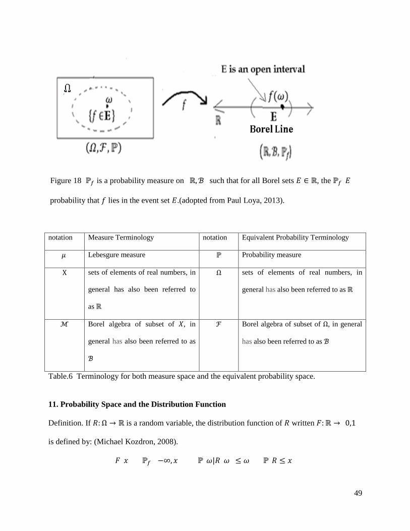
Figure 18 ℙ𝑓𝑓 is a probability measure on (ℝ,ℬ) such that for all Borel sets 𝐸𝐸 ∈ ℝ, the ℙ𝑓𝑓(𝐸𝐸) =
probability that 𝑓𝑓 lies in the event set 𝐸𝐸.(adopted from Paul Loya, 2013).
notation Measure Terminology notation Equivalent Probability Terminology
𝜇𝜇 Lebesgure measure ℙ Probability measure
X sets of elements of real numbers, in
general has also been referred to
as ℝ
Ω sets of elements of real numbers, in
general has also been referred to as ℝ
ℳ Borel algebra of subset of 𝑋𝑋, in
general has also been referred to as
ℬ
ℱ Borel algebra of subset of Ω, in general
has also been referred to as ℬ
Table.6 Terminology for both measure space and the equivalent probability space.
11. Probability Space and the Distribution Function
Definition. If 𝑅𝑅:Ω → ℝ is a random variable, the distribution function of 𝑅𝑅 written 𝐹𝐹:ℝ → [0,1]
is defined by: (Michael Kozdron, 2008).
𝐹𝐹(𝑥𝑥) = ℙ𝑓𝑓{(−∞,𝑥𝑥])} = ℙ{𝜔𝜔|𝑅𝑅(𝜔𝜔) ≤ 𝜔𝜔} = ℙ{𝑅𝑅 ≤ 𝑥𝑥}

50
For every 𝑥𝑥 ∈ ℝ.
𝑅𝑅(random variable) ↭ℙ𝑓𝑓(law of 𝑅𝑅) ↭ 𝐹𝐹(distribution function of 𝑅𝑅)
Theorem: If 𝐹𝐹 is a nondecreasing, right-continuous function satisfying lim𝑥𝑥→∞+
𝐹𝐹(𝑥𝑥) = 1 and
lim𝑥𝑥→−∞−
𝐹𝐹(𝑥𝑥) = 0, then there exist on some probability space a random variable R for which
𝐹𝐹(𝑥𝑥) = ℙ[𝑅𝑅 ≤ 𝑥𝑥]. (Patrick Billingsley, 1995)
Proof: (by Patrick Billingsley, 1995)
For the probability space, take (Ω,ℱ,ℙ) = (ℝ,ℬ, 𝜇𝜇), the open unit interval Ω is (0,1), ℱ consists
of the Borel subsets of (0,1), and ℙ(𝐸𝐸) = 𝜇𝜇(𝐸𝐸) is Lebesgue measure of 𝐸𝐸. To understand the
method, suppose at first that 𝐹𝐹 is continuous and strictly increasing. Then 𝐹𝐹 is a one-to-one
mapping of ℝ onto (0,1); let 𝜑𝜑: (0,1) → ℝ, be the inverse mapping. For 0 < 𝜔𝜔 < 1, let 𝑅𝑅(𝜔𝜔) =
𝜑𝜑(𝜔𝜔). Since 𝜑𝜑 is increasing, certainly 𝑅𝑅 is measurable ℱ. If 0 < 𝑠𝑠 < 1, then 𝜑𝜑(𝑠𝑠) ≤ 𝑥𝑥 if and
only if 𝑠𝑠 ≤ 𝐹𝐹(𝑥𝑥). Since ℙ is a Lebesgue measure, ℙ[𝑅𝑅 ≤ 𝑥𝑥] = ℙ[𝜔𝜔 ∈ (0,1)|𝜑𝜑(𝜔𝜔) ≤ 𝑥𝑥] =
ℙ[𝜔𝜔 ∈ (0,1)|𝜔𝜔 ≤ 𝐹𝐹(𝑥𝑥)] = 𝐹𝐹(𝑥𝑥) as required.
If 𝐹𝐹 has discontinuities or is not strictly increasing, it is defined as follows:
𝜑𝜑(𝑠𝑠) = 𝐻𝐻𝑎𝑎𝑓𝑓[𝑥𝑥|𝑠𝑠 ≤ 𝐹𝐹(𝑥𝑥)]
For 0 < 𝑠𝑠 < 1. Since 𝐹𝐹 is nondecreasing, [𝑥𝑥|𝑠𝑠 ≤ 𝐹𝐹(𝑥𝑥)] is an interval stretching to ∞; since 𝐹𝐹 is
right continuous, this interval is closed on the left. For 0 < 𝑠𝑠 < 1, therefore, [𝑥𝑥|𝑠𝑠 ≤ 𝑓𝑓(𝑥𝑥)] =
[𝜑𝜑(𝑠𝑠),∞] and so 𝜑𝜑(𝑠𝑠) ≤ 𝑥𝑥 if and only if 𝑠𝑠 ≤ 𝐹𝐹(𝑥𝑥). If 𝑅𝑅(𝜔𝜔) = 𝜑𝜑(𝜔𝜔) for 0 < 𝜔𝜔 < 1, then by
the same reasoning as before, 𝑅𝑅 is a random variable and ℙ[𝑅𝑅 ≤ 𝑥𝑥] = 𝐹𝐹(𝑥𝑥).

51
(adpoted from: Patrick Billingsley,1995)
This provides a simple proof for the probability distribution 𝐹𝐹.(Patrick Billingsley, 1995).
The constructed distribution 𝐹𝐹(𝑥𝑥) that defined by 𝜇𝜇(𝐸𝐸) = ℙ[𝑅𝑅 ∈ 𝐸𝐸] for 𝐸𝐸 ∈ ℬ satisfies
𝜇𝜇(−∞,𝑥𝑥] = 𝐹𝐹(𝑥𝑥) and hence 𝜇𝜇(𝑎𝑎,𝑏𝑏] = 𝐹𝐹(𝑏𝑏) − 𝐹𝐹(𝑎𝑎).
12. Lebesgue-Stieltjes Measure
Definition. Assume 𝜇𝜇 is a finite Borel measure on ℝ and let 𝐹𝐹(𝑥𝑥) = 𝜇𝜇�(−∞,𝑥𝑥]� = 𝜇𝜇(𝐸𝐸), in
which 𝜇𝜇(𝐸𝐸) is the length of the interval (𝑎𝑎,𝑏𝑏] and therefore 𝜇𝜇 = Lebesgue measure on ℬ, then 𝐹𝐹
is the distribution function of 𝜇𝜇. The measure 𝜇𝜇𝐹𝐹 is called the Lebesgue-Stieltjes measure
associated with 𝐹𝐹. (adopted from Kyle Siegrist, 2015)
The Lebesgue Stieltjes measure 𝜇𝜇𝐹𝐹 induced by a distribution function 𝐹𝐹 is the measure defined
𝜇𝜇𝐹𝐹(𝑎𝑎,𝑏𝑏] = 𝐹𝐹(𝑏𝑏) − 𝐹𝐹(𝑎𝑎) for interval (𝑎𝑎,𝑏𝑏] and for other Borel sets on the real line by the method
of measure extension. (A. K. Basu, 2012).
Definition. 𝒫𝒫(𝑋𝑋) denote the set of all subset of 𝑋𝑋 , and for 𝒜𝒜 ⊆ ℝ,
𝜇𝜇(𝒜𝒜) = inf ���𝐹𝐹(𝑏𝑏𝑖𝑖 −) − 𝐹𝐹(𝑎𝑎𝑖𝑖 +)��∞
𝑖𝑖=1
𝒜𝒜 ⊆�(𝑎𝑎𝑖𝑖, 𝑏𝑏𝑖𝑖)∞
𝑖𝑖=1
�

52
Which means, we look at all covering of 𝒜𝒜 with open intervals and for each of these open
covering, we add the length of the individual open intervals and take the infimum of all such
numbers obtained. (Kuttler, 2014). The Lebesgue-Stieltjes measure is considered as a
generalization of one dimensional Lebesgue measure.
12.1 Lebesgue-Stieltjes Measure as a Model for Distributions
The measure 𝜇𝜇 that associates with the distribution function 𝐹𝐹 on ℝ is Lebesgue-Stieltjes
measure and has the following properties:
i. increasing [𝑎𝑎 < 𝑏𝑏 𝐻𝐻𝑚𝑚𝑝𝑝𝑎𝑎𝐻𝐻𝑒𝑒𝑠𝑠 𝐹𝐹(𝑎𝑎) ≤ 𝐹𝐹(𝑏𝑏)] and
ii. right continuous �lim𝑥𝑥→𝑥𝑥0+ 𝐹𝐹(𝑥𝑥) = 𝐹𝐹(𝑥𝑥0)�.
The Lebesgue-Stieltjes measure is a Borel measure on ℝ which assume finite values on
compact set (Rudi Weikard, 2016), and if the function 𝐹𝐹 is to be defined as a Borel measure
we need
𝑎𝑎𝐻𝐻𝑚𝑚𝑖𝑖→∞
𝜇𝜇𝐹𝐹 ��𝑎𝑎,𝑎𝑎 +1𝐻𝐻�� = lim
𝑖𝑖→∞�𝐹𝐹 �𝑎𝑎 +
1𝐻𝐻� − 𝐹𝐹(𝑎𝑎)� = lim
𝑥𝑥→𝑎𝑎+𝐹𝐹(𝑥𝑥) − 𝐹𝐹(𝑎𝑎) = 0
where 𝑎𝑎+ = lim∆→0(𝑎𝑎 + ∆), that is 𝐹𝐹(𝑥𝑥) is continuous to the right.
The formula 𝜇𝜇𝐹𝐹(𝑎𝑎,𝑏𝑏] = 𝐹𝐹(𝑏𝑏) − 𝐹𝐹(𝑎𝑎) sets up a one to one correspondence between Lebesgue-
Stieltjes measures and distribution functions, where two distribution functions that differ by a
constant are identified.
13. Properties of the Distribution Function
Theorem.The distribution function of 𝐹𝐹(𝑥𝑥) of a random variable 𝑅𝑅 has the following properties:
(Roman Vershynin, 2008)
i. 𝐹𝐹 is nondecreasing and 0 ≤ 𝐹𝐹 ≤ 1

53
𝐹𝐹(𝑥𝑥) → 1 as 𝑥𝑥 → ∞, i.e., lim𝑥𝑥→∞+
𝐹𝐹(𝑥𝑥) = 1
𝐹𝐹(𝑥𝑥) → 0 as 𝑥𝑥 → −∞, i.e., lim𝑥𝑥→∞−
𝐹𝐹(𝑥𝑥) = 0
ii. 𝐹𝐹(𝑥𝑥 −) = ℙ(𝑅𝑅 < 𝑥𝑥), 𝑥𝑥 ∈ ℝ and 𝐹𝐹 has limit from the left
iii. 𝐹𝐹(𝑥𝑥 +) = 𝐹𝐹(𝑥𝑥), 𝑥𝑥 ∈ ℝ and 𝐹𝐹 is continuous from the right
F has left hand limits at all points (these are jumps on the distribution function, and
these jumps mean the probability that R takes this specific value).
Suppose 𝐹𝐹 is the distribution function of a real-valued random variable, if 𝑎𝑎, 𝑏𝑏 ∈ ℝ and 𝑎𝑎 < 𝑏𝑏
then: (adopted from Kyle Siegrist, 2015).
𝜇𝜇{𝑎𝑎} = ℙ(𝑅𝑅 = 𝑎𝑎) = 𝐹𝐹(𝑎𝑎) − 𝐹𝐹(𝑎𝑎−)
𝜇𝜇(𝑎𝑎, 𝑏𝑏] = ℙ(𝑎𝑎 < 𝑅𝑅 ≤ 𝑏𝑏) = 𝐹𝐹(𝑏𝑏) − 𝐹𝐹(𝑎𝑎)
𝜇𝜇(𝑎𝑎, 𝑏𝑏) = ℙ(𝑎𝑎 < 𝑅𝑅 < 𝑏𝑏) = 𝐹𝐹(𝑏𝑏 −) − 𝐹𝐹(𝑎𝑎)
𝜇𝜇[𝑎𝑎. 𝑏𝑏] = ℙ(𝑎𝑎 ≤ 𝑅𝑅 ≤ 𝑏𝑏) = 𝐹𝐹(𝑏𝑏) − 𝐹𝐹(𝑎𝑎−)
𝜇𝜇[𝑎𝑎, 𝑏𝑏) = ℙ(𝑎𝑎 ≤ 𝑅𝑅 < 𝑏𝑏) = 𝐹𝐹(𝑏𝑏 −) − 𝐹𝐹(𝑎𝑎−)
Distribution function 𝐹𝐹(𝑥𝑥) has Left hand limit and right continuous
(adopted from Kyle Siegrist, 2015) (adopted from Ali Hussien Muqaibel)

54
14. Relate the Measure 𝝁𝝁 to the Distribution Function, 𝑭𝑭
The distribution of 𝑅𝑅 is determined by its value of the form ℙ(𝑅𝑅 ∈ 𝐸𝐸),𝐸𝐸 = (−∞,𝑥𝑥], 𝑥𝑥 ∈ ℝ
because such intervals form a generating collection of ℱ and measure is uniquely determined by
its value on a collection of generators, 𝑅𝑅 = 𝜎𝜎�(−∞, 𝑥𝑥], 𝑥𝑥 ∈ ℝ� .
Consider the probability space defined as (Ω,ℱ, 𝜇𝜇) where Ω is a set, ℱ is a Borel algebra of
subset of Ω, and 𝜇𝜇:ℱ → ℝ a probability measure. The law of a random variable is always a
probability measure on (ℝ,ℬ), thus the distribution function induced by 𝜇𝜇 is the function
𝐹𝐹:ℝ → [0,1] defined by:
𝐹𝐹(𝑥𝑥) = 𝜇𝜇{(−∞, 𝑥𝑥)} ∀ 𝑥𝑥 ∈ ℝ
and, since
(−∞,𝑥𝑥] = ��−∞, 𝑥𝑥 +1𝑎𝑎�
∞
𝑛𝑛=1
is the countable intersection of open sets, we see that (−∞,𝑥𝑥] ∈ ℬ for every 𝑥𝑥 ∈ ℝ. Thus
𝜇𝜇{(−∞, 𝑥𝑥]} make sense. (Michael Kozdron, 2008).
15. Distribution Function on ℝ𝒏𝒏
Proposition. If 𝑅𝑅1, … ,𝑅𝑅𝑛𝑛 are random variables, the (𝑅𝑅1, … ,𝑅𝑅𝑛𝑛) is a random vector.(Roman
Vershynin, 2008).
We can generalize the construction to many random variables 𝑅𝑅1, … ,𝑅𝑅𝑛𝑛, once we know
𝐹𝐹(𝑥𝑥1, … 𝑥𝑥𝑛𝑛) = 𝜇𝜇𝐹𝐹(𝑅𝑅1 ≤ 𝑥𝑥1, … ,𝑅𝑅𝑛𝑛 ≤ 𝑥𝑥𝑛𝑛). In this case Ω = ℝ𝑛𝑛, ℱ = Borel algebra generated by
open sets of ℝ𝑛𝑛. (Joseph G. Conlon, 2010).
Further generalized to countably infinite set of variables 𝑅𝑅1,𝑅𝑅2, …, provided the distribution of
the variables satisfy an obvious consistency condition. Thus for

55
1 ≤ 𝑗𝑗1 < 𝑗𝑗2 < ⋯ < 𝑁𝑁𝑗𝑗
Let 𝐹𝐹𝑗𝑗1,𝑗𝑗2,…,𝑗𝑗𝑁𝑁(𝑥𝑥1,𝑥𝑥2, 𝑥𝑥𝑁𝑁) be the distribution of 𝑅𝑅𝑗𝑗1,𝑅𝑅𝑗𝑗2, … ,𝑅𝑅𝑗𝑗𝑁𝑁. Consistency then just means:
lim𝑥𝑥𝑘𝑘→∞
𝐹𝐹𝑗𝑗1,𝑗𝑗2,…,𝑗𝑗𝑁𝑁(𝑥𝑥1,𝑥𝑥2, … 𝑥𝑥𝑘𝑘−1,𝑥𝑥𝑘𝑘 , 𝑥𝑥𝑘𝑘+1, … , 𝑥𝑥𝑁𝑁)
= 𝐹𝐹𝑗𝑗1,𝑗𝑗2,…,𝑗𝑗𝑘𝑘−1,𝑗𝑗𝑘𝑘+1,…,𝑗𝑗𝑁𝑁 (𝑥𝑥1,𝑥𝑥2, … 𝑥𝑥𝑘𝑘−1,𝑥𝑥𝑘𝑘 , 𝑥𝑥𝑘𝑘+1, … , 𝑥𝑥𝑁𝑁)
for all possible choice of the 𝑗𝑗𝑖𝑖 ≥ 1, 𝑥𝑥𝑖𝑖 ∈ ℝ. Here 𝛺𝛺 = ℝ∞ and ℱ is the 𝜎𝜎-field generated by
finite dimensional rectangles.
The notion of a distribution function on ℝ𝑛𝑛, 𝑎𝑎 ≥ 2, is more complicated than the one
dimensional case, and we may work with compact space ℝ, that includes the (−∞,∞).
Let 𝑎𝑎 = 3, and let 𝜇𝜇 be finite measure on ℬ(ℝ3), then
𝐹𝐹(𝑥𝑥1, 𝑥𝑥2, 𝑥𝑥3) = 𝜇𝜇{𝜔𝜔 ∈ ℝ3: 𝜔𝜔1 ≤ 𝑥𝑥1, 𝜔𝜔2 ≤ 𝑥𝑥2, 𝜔𝜔3 ≤ 𝑥𝑥3}, (𝑥𝑥1,𝑥𝑥2, 𝑥𝑥3) ∈ ℝ3
By analogy with the one-dimensional case, we expect that F is a distribution function
corresponding to 𝜇𝜇. The formula 𝜇𝜇𝐹𝐹(𝑎𝑎, 𝑏𝑏] = 𝐹𝐹(𝑏𝑏) − 𝐹𝐹(𝑎𝑎) will be replaced by:
𝜇𝜇𝐹𝐹(𝑎𝑎, 𝑏𝑏] = ∆𝑏𝑏1𝑎𝑎1 ∆𝑏𝑏2𝑎𝑎2∆𝑏𝑏3𝑎𝑎3𝐹𝐹(𝑥𝑥1, 𝑥𝑥2, 𝑥𝑥3)
where ∆ is the difference operator,
Our operation is introduced as follows:
If 𝐺𝐺: ℝ𝑛𝑛 → ℝ,∆𝑏𝑏𝑖𝑖𝑎𝑎𝑖𝑖 𝐺𝐺(𝑥𝑥1, … 𝑥𝑥𝑛𝑛) is defined as
𝐺𝐺(𝑥𝑥1, … , 𝑥𝑥𝑖𝑖−1, 𝑏𝑏𝑖𝑖, 𝑥𝑥𝑖𝑖+1, … , 𝑥𝑥𝑛𝑛) − 𝐺𝐺(𝑥𝑥1, … , 𝑥𝑥𝑖𝑖−1,𝑎𝑎𝑖𝑖, 𝑥𝑥𝑖𝑖+1, … , 𝑥𝑥𝑛𝑛)
Lemma. If 𝑎𝑎 ≤ 𝑏𝑏, that is, 𝑎𝑎𝑖𝑖 ≤ 𝑏𝑏𝑖𝑖, 𝐻𝐻 = 1,2,3 then
𝜇𝜇𝐹𝐹(𝑎𝑎, 𝑏𝑏] = ∆𝑏𝑏1𝑎𝑎1 ∆𝑏𝑏2𝑎𝑎2∆𝑏𝑏3𝑎𝑎3𝐹𝐹(𝑥𝑥1, 𝑥𝑥2, 𝑥𝑥3)
Where

56
∆𝑏𝑏1𝑎𝑎1 ∆𝑏𝑏2𝑎𝑎2∆𝑏𝑏3𝑎𝑎3𝐹𝐹(𝑥𝑥1, 𝑥𝑥2, 𝑥𝑥3)
= 𝐹𝐹(𝑏𝑏1, 𝑏𝑏2, 𝑏𝑏3) − 𝐹𝐹(𝑎𝑎1,𝑏𝑏2, 𝑏𝑏3) − 𝐹𝐹(𝑏𝑏1,𝑎𝑎2, 𝑏𝑏3) − 𝐹𝐹(𝑏𝑏1,𝑏𝑏2,𝑎𝑎3) + 𝐹𝐹(𝑎𝑎1,𝑎𝑎2, 𝑏𝑏3)
+ 𝐹𝐹(𝑎𝑎1,𝑏𝑏2,𝑎𝑎3) + 𝐹𝐹(𝑏𝑏1,𝑎𝑎2,𝑎𝑎3) − 𝐹𝐹(𝑎𝑎1,𝑎𝑎2,𝑎𝑎3) ≥ 0
Thus 𝜇𝜇𝐹𝐹(𝑎𝑎, 𝑏𝑏] is not simply 𝐹𝐹(𝑏𝑏) − 𝐹𝐹(𝑎𝑎)
Figure 19 Cartesian product of 𝜇𝜇�(𝑎𝑎1,𝑏𝑏1] × (𝑎𝑎2,𝑏𝑏2]) .(source: A. K. BASU, 2012)
Non Example. (adopted from Rick Durrett, 2013)
Given 𝐹𝐹(𝑥𝑥,𝑦𝑦) as below:
𝐹𝐹(𝑥𝑥,𝑦𝑦) = �
1 𝐻𝐻𝑓𝑓 𝑥𝑥, 𝑦𝑦 ≥ 12/3 𝐻𝐻𝑓𝑓 𝑥𝑥 ≥ 1 𝑎𝑎𝑎𝑎𝑑𝑑 0 ≤ 𝑦𝑦 < 12/3 𝐻𝐻𝑓𝑓 𝑦𝑦 ≥ 1 𝑎𝑎𝑎𝑎𝑑𝑑 0 ≤ 𝑥𝑥 < 1
0 𝑛𝑛𝑜𝑜ℎ𝑒𝑒𝑟𝑟𝑤𝑤𝐻𝐻𝑠𝑠𝑒𝑒
Figure 20 Non Example (adopted from Rick Durrett, 2013)

57
Suppose 𝐹𝐹 gives rise to a measure 𝜇𝜇 on ℝ2, 𝐹𝐹:ℝ2 → ℝ is right continuous, i.e.
𝐹𝐹(𝑎𝑎, 𝑏𝑏) = 𝜇𝜇((−∞ ,𝑎𝑎] . (−∞ , 𝑏𝑏])
F is increasing: if 𝑥𝑥 ≤ 𝑦𝑦 then 𝐹𝐹(𝑥𝑥) ≤ 𝐹𝐹(𝑦𝑦)
o 𝐹𝐹(𝑥𝑥 +) = 𝐹𝐹(𝑥𝑥) 𝑓𝑓𝑛𝑛𝑟𝑟 𝑥𝑥 ∈ ℝ and 𝐹𝐹 is continuous from the right
o 𝐹𝐹(𝑥𝑥 −) = ℙ(𝑋𝑋 < 𝑥𝑥) 𝑓𝑓𝑛𝑛𝑟𝑟 𝑥𝑥 ∈ ℝ and F has limits from the left
o 𝐹𝐹(−∞) = 0
o 𝐹𝐹(∞) = 1
Figure 21 Solution for Non Example (Dr. Seshendra Pallekonda, 2015)
From the Cartesian product of 𝜇𝜇�(𝑎𝑎1,𝑏𝑏1] × (𝑎𝑎2,𝑏𝑏2]) we have.
𝜇𝜇𝐹𝐹(𝑎𝑎, 𝑏𝑏] = 𝐹𝐹(𝑏𝑏1,𝑏𝑏2) − 𝐹𝐹(𝑎𝑎1,𝑏𝑏2) − 𝐹𝐹(𝑏𝑏1,𝑎𝑎2) + 𝐹𝐹(𝑎𝑎1,𝑎𝑎2) ≥ 0
Then

58
𝜇𝜇�(𝑎𝑎1,𝑏𝑏1] × (𝑎𝑎2,𝑏𝑏2])
= 𝜇𝜇�(−∞, 𝑏𝑏1] × (−∞, 𝑏𝑏2]) − 𝜇𝜇�(−∞,𝑎𝑎1]
× �−∞, 𝑏𝑏2]) − 𝜇𝜇�(−∞,𝑏𝑏1] × (−∞,𝑎𝑎2]) +𝜇𝜇�(−∞,𝑎𝑎1] × (−∞,𝑎𝑎2])
= 𝐹𝐹(𝑏𝑏1,𝑏𝑏2) − 𝐹𝐹(𝑎𝑎1,𝑏𝑏2) − 𝐹𝐹(𝑏𝑏1,𝑎𝑎2) + 𝐹𝐹(𝑎𝑎1,𝑎𝑎2)
Let 𝑎𝑎1 = 𝑎𝑎2 = 1 − 𝜀𝜀 and 𝑏𝑏1 = 𝑏𝑏2 = 1 and letting 𝜀𝜀 → 0
lim𝜀𝜀→0
𝜇𝜇((1− 𝜀𝜀, 1] × (1 − 𝜀𝜀, 1])
= lim𝜀𝜀→0
𝐹𝐹(1,1) − lim𝜀𝜀→0
𝐹𝐹(1 − 𝜀𝜀, 1) − lim𝜀𝜀→0
𝐹𝐹(1,1 − 𝜀𝜀) + lim𝜀𝜀→0
𝐹𝐹(1 − 𝜀𝜀, 1 − 𝜀𝜀)
Using 𝑎𝑎1 = 𝑎𝑎2 = 1 − 𝜀𝜀 and 𝑏𝑏1 = 𝑏𝑏2 = 1 and letting 𝜀𝜀 → 0
𝜇𝜇({1,1}) = 1 −23−
23
+ 0 = −13
𝑤𝑤ℎ𝐻𝐻𝑐𝑐ℎ 𝐻𝐻𝑠𝑠 < 0
𝜇𝜇({1,0}) = 𝜇𝜇({0,1}) =23
𝜇𝜇({1,1}) = −13
< 0

59
CONCLUSION IN GENERAL
Measure theory is foundation of probability and probabilities are special sorts of measures. The
probability uses unlike terminology than that of measure but one can notice the similarity in the
definition of measurable functions, and the Borel measure, in both theory or spaces.
In fact learning the main concept of measure theory as probability theory is easier than
understanding this concept through real analysis. The reason is that probability is rich in applied
examples beside the description of the probability jargon noteworthy pictured the idea rather
than in real analysis or measure theory do. Thus most of the books about the measure theory
consider the probability thought with the measure analysis.
The study includes a list of the measure, probability and topology components (elements) and
examines the structure of their triple spaces in order to relate each one to the other. The measure
can be written in different ways and the idea of the triple space is the same thus it can be applied
to variety of fields of science, and it is not the matter if each one has driven from the other, it is
the matter of how to use and understand the component of the structure.
To complete the conclusion I should thank all the writers, who make their science resources
available online, that I used on forming this topic and hoping that this material has been
assembled with minor mistake.

60
REFERENCES
Auyang, S. Y. (1995). How is Quantum Field Theory Possible? Oxford university press.
Basu, A. K. (2012). Measure Theory and Probability. Delhi: Asoke K. Ghosh.
Billingsley, P. (1995). Probability and Measure, 3rd Edition, University of Chicago. John Wiley
& Sons.
Bradley, T.-D. (2015). The Borel-Cantelli Lemma. Retrieved from Mathema:
http://www.math3ma.com/mathema/2015/9/21/the-borel-cantelli-lemma
Cheng, S. (April 27, 2008). A crash Course on the Lebesgue Integral and Measure Theory.
Retrieved 2016, from http://www.gold-saucer.org/math/lebesgue/lebesgue.pdf
Chernov, N. (2012-2014). Teaching by Nikolai Chernov at University of Alabama at
Birmingham. Retrieved from Real Analysis, MA 646-2F :
http://people.cas.uab.edu/~mosya/teaching/teach.html
Durrett, R. ( April 21, 2013). Probability: Theory and Examples, Edition 4.1. Cambridge
University Press in 2010.
Epps, T. W. (2014). Probability and Statistical Theory for Appiled Researchers, university of
Virgina, USA. World Scientific.
Etnyre, J. B. (2014). Recollections from point set topology and overview of quotient spaces.
Retrieved 2016, from Georgia Institute of Technology:
http://people.math.gatech.edu/~etnyre/class/6452Fall14/TopologyReview.pdf
Folland, G. B. (1999). Real Analysis, Modern Techiques and Their Application, 2nd Edition.
John Wiley & Sons Inc.
G.Conlon, J. (2010, 12 17). Math 625, Probability and Random Processes. Retrieved 2016, from
University of Michigan: http://www.math.lsa.umich.edu/~conlon/math625/chapter1.pdf
Garside, B. (2014, Oct). functional analysis. Retrieved Sep 2015, from
https://www.youtube.com/playlist?list=PLAvgI3H-gclZa-DVTMyUIAxM-X8NSikwu
Garside, S. B. (2014, Sep 5). Introduction to Metric Spaces. Retrieved from
https://www.youtube.com/watch?v=etP21xln8iQ
Genovese, C. (2006, spring). Intermediate Probability. Retrieved from Carnegie Mellon
University: http://www.stat.cmu.edu/~genovese/class/iprob-S06/

61
Grigoryan, A. (2007-2008). Measure Theory and Probability. Retrieved from Lecture Notes,
University of Bielefeld: https://www.math.uni-bielefeld.de/~grigor/mwlect.pdf
Herzong, F. (2013). Probability Theory. Retrieved from
https://www.ethz.ch/content/dam/ethz/special-interest/mavt/dynamic-systems-n-
control/idsc-dam/Lectures/Stochastic-Systems/Probability.pdf
Hoffman-Jorgensen, J. (1994). Probability With a View Towards Statistics. Chapman & Hall.
Jayasumana, S. (2012, June 11). Sadeep's Tech Blog. Retrieved from Blogger:
http://sadeepj.blogspot.com/2012/06/understanding-riemannian-manifolds-part.html
Kannan, V. D. (n.d.). Measure Theory for Applied Research. Retrieved Oct 31, 2015, from
https://www.youtube.com/channel/UCFwohpuBUlR3gdkJq3bn6_Q
Kannan, V. D. (n.d.). Measure Theory for Applied Research. Retrieved 2015, from Measurable
Functions: https://www.youtube.com/watch?v=JoL0b6Az2CY
Kozdron, M. (winter 2008). University of British Columbia. Retrieved cited 2016, from Lecture
Notes: http://stat.math.uregina.ca/~kozdron/
Kuttler. (2014, 3 21). Real and Abstract Analysis. Retrieved 2016, from Lecture Notes:
https://www.math.byu.edu/~klkuttle/541book.pdf
Leadbetter, R., Cambanis , S., & Pipiras, V. (2014). A Basic Course in Measure and Probability:
Theory for Applications, 1st Ed. Cambridge university press.
Lebl, J. (2011, Fall). Basic Analysis: Introduction to Real Analysis. Retrieved 2015, from
University of Pittsburgh supplements: http://www.math.pitt.edu/~frank/pittanal2121.pdf
Loya, P. (2013). Lebesgue's Remarkable Theory of Measure and Integration with Probability.
Retrieved cited 2016, from Binghamton university:
http://www.math.binghamton.edu/loya/479-S13/Loyabook.pdf
MIT. (Fall 2008). Massachusetts Institute of Technology. Retrieved 2016, from Fundamentals of
Probability, 6.436J / 15.085J, Lecture2: http://ocw.mit.edu/courses/electrical-
engineering-and-computer-science/6-436j-fundamentals-of-probability-fall-2008/lecture-
notes/
Morais, M. C. (2009-2010). Lecture Notes - Probability Theory. In I. S. Tecnico.
Muqaibel, A. H. (2016, Mar 6). SlideShare. Retrieved from Random Variables Dr. Ali Hussein
Muqaibel Ver. 2.3 1: http://www.slideshare.net/MuhannadSaleh/2-random-variables-
notes-2p3

62
Nagy, G. (FALL 2001). Notes in One File. Retrieved from REAL ANALYSIS, Kansas State
University: https://www.math.ksu.edu/~nagy/real-an/real-an-old/notes.pdf
Norris, J. (2010). Probability and Measure. Retrieved from
http://www.statslab.cam.ac.uk/~james/Lectures/pmall.pdf
Omer, P. (2012, Dec 3). Probability and Random Variables. Retrieved from
http://www.slideshare.net/pratomer/ch2-probability-and-random-variables-pg-81
Pallekonda, S. (2015, Dec). Senior Research Analyst . Idaho Department Of Labor.
Porter, F. (n.d.). The Jordan Measure. Retrieved cited 2016, from Physics 129a, Measure
Theory: http://www.hep.caltech.edu/~fcp/math/measureTheory/measureTheory.pdf
Pra, P. D. (cited 2016). Basic Measure Theory. Retrieved from University of Padua:
http://www.math.unipd.it/~daipra/didattica/galileiana-15/Parte-I.pdf
Quibb. (2013). Lebesgue Measure. Retrieved cited 2016, from Professor Quibb:
http://quibb.blogspot.com/2013/02/lebesgue-measure.html
RJS. (2012, 1 28). University of Texas at Dallas. Retrieved from Some Basic Classes of Subsets
of a Space X: http://www.utdallas.edu/~serfling/handouts/SomeBasicClassesOfSets.pdf
Royden, H. L. (1988). Real Anaylsis, 3rd Edition. Prentive-Hall, Inc.
Royden, H., & Fitzpatrick, P. M. (2010). Real Analysis, 4th Edition. Prentice Hall.
Saks, S. (2016). Home Page of Stefan Banach. Retrieved from Theory of the Integral, with
additional notes by Stefan Banach: http://kielich.amu.edu.pl/Stefan_Banach/e-saks.html
Satish, S., & Harkrishan, V. L. (2011). Multivariable Analysis. Springer-Verlag London Limited.
Shen, J. (2012). School of Economics, The University of New South Wales, Australia. Retrieved
from Mathematics for Economics and Finance, Lecture Notes (14/02/2012):
http://jianfeishen.weebly.com/uploads/4/7/2/6/4726705/math2012.pdf
Siegrist, K. (1997-2015). Probability Convergence. Retrieved from University Alabama:
http://www.math.uah.edu/stat/prob/Convergence.html#con
Susmel, R. (8/2015). Bauer College of Business. Retrieved from
http://www.bauer.uh.edu/rsusmel/phd/sR-0.pdf.
Swartz, C. (1994). Measure, Integration and function Space. World scientific publishing .
Tarantola, A. (2007). Mapping of Probabilities Theory for the Interpretation of Uncertain
Physical Measurements. Cambridge University Press.

63
Tarantola, A. (2007). Mapping of Probabilities Theory for the Interpretation of Uncertain
Physical Measurements .
Thomson, B. S., Bruchner, J. B., & Bruchner, A. M. (2008). Elementary Real Analysis. Prentice
Hall.
UF. (Fall 2012). University of Florida College of Liberal Arts and Sciences,. Retrieved from
MAA6616 Course Notes : http://people.clas.ufl.edu/mjury/files/6616notesshort.pdf
Valkó, B. (2015). Introduction to the Theory of Probability. Retrieved from Math/Stat 431:
http://www.math.wisc.edu/~valko/courses/431/431.html
Vershynin, R. (2007-2008). MAT 235A / 235B: Probability, UM Personal World Wide Web
Server . Retrieved 2016, from Lecture Notes in Probability Theory, Function of Random
Variables: http://www-personal.umich.edu/~romanv/teaching/2007-08/235B/lecture-
notes.pdf
Weikard, R. (2016, Feb 29). Real Analysis. Retrieved from Lecture notes for MA 645/646:
http://people.cas.uab.edu/~weikard/teaching/reals.pdf
Weisstein, E. (2015). Vector Norm, (creator of MathWorld). Retrieved 2015, from Created,
developed, and nurtured by Eric Weisstein at Wolfram Research:
http://mathworld.wolfram.com/Norm.html
Wikipedia. (n.d.). Probability Measure. Retrieved 2014, from
https://en.wikipedia.org/wiki/Probability_measure
William, J. (2015). The Lebesgue Integral for Undergraduates. The Mathematical Association of
America.