a logic for reasoning about probabilities*theory.stanford.edu/~megiddo/pdf/fag-hal.pdf · than that...
TRANSCRIPT

Reprinted from INFORMATION AND COMPUTATION All Rights Reserved by Academic Press. New York and London
V o l . 87, N o s I/2, July/August 1990 Printed in Belgium
A Logic for Reasoning about Probabilities*
IBM Almaden Research Center, San Jose, California 95120
We consider a language for reasoning about probability which allows us to make statements such as "the probability of El is less than f" and "the probability of E , is at least twice the probability of E,," where E, and E, are arbitrary events. We consider the case where all events are measurable (i.e., represent measurable sets) and the more general case, which is also of interest in practice, where they may not be measurable. The measurable case is essentially a formalization of (the proposi- tional fragment of) Nilsson's probabilistic logic. As we show elsewhere, the general (nonmeasurable) case corresponds precisely to replacing probability measures by Dempster-Shafer belief functions. In both cases. we provide a complete axiomatiza- tion and show that the problem of deciding satisfiability is NP-complete, no worse than that of propositional logic. As a tool for proving our complete axiomatiza- tions, we give a complete axiomatization for reasoning about Boolean combina- tions of linear inequalities, which is of independent interest. This proof and others make crucial use of results from the theory of linear programming. We then extend the language to allow reasoning about conditional probability and show that the resulting logic is decidable and completely axiomatizable, by making use of the theory of real closed fields. C 1990 Acddemlc Press, Inc
The need for reasoning about probability arises in many areas of research. In computer science we must analyze probabilistic programs, reason about the behavior of a program under probabilistic assumptions about the input, or reason about uncertain information in an expert system. While probability theory is a well-studied branch of mathematics, in order to carry out formal reasoning about probability, it is helpful to have a logic for reasoning about probability with a well-defined syntax and semantics. Such a logic might also clarify the role of probability in the analysis: it is all too easy to lose track of precisely which events are being assigned probability, and how that probability should be assigned (see [HT89] for a discussion of the situation in the context of distributed systems). There is a fairly extensive literature on reasoning about probabil-
* A preliminary version of this paper appeared in the Proceedings of the 3rd IEEE 1988 Symposium on Logic in Computer Science, pp. 2777291.
78 0890-5401/90 $3.00 Copyr~ght I 1990 by Academ~c Pres. l n c All r~ghts of reproductmn ~n any lorm resenrd
LOGIC FOR REASONING ABOUT PROBABILITIES 79
ity (see, for example, [Bac88, CarSO, Gai64, GKP88, GF87, HF87, Hoo78, Kav88, Kei85, Luk70, Ni186, Nut87, Sha761 and the references in [Ni186]), but there are remarkably few attempts at constructing a logic to reason explicitly about probabilities.
We start by considering a language that allows linear inequalities involving probabilities. Thus, typical formulas include 3w(cp) < 1 and w(cp)>,2w($). We consider two variants of the logic. In the first, cp and i,b represent measurable events, which have a well-defined probability. In this case, these formulas can be read "three times the probability of cp is less than one" (i.e., cp has probability less than f) and "cp is at least twice as probable as i,b." However, at times we want to be able to discuss in the language events that are not measurable. In such cases, we view w(cp) as representing the inner measure (induced by the probability measure) of the set corresponding to q. The letter 11: is chosen to stand for "weight"; w will sometimes represent a (probability) measure and sometimes an inner measure induced by a probability measure.
Mathematicians usually deal with nonmeasurable sets out of mathemati- cal necessity: for example, it is well known that if the set of points in the probability space consists of all numbers in the real interval [0, 11, then we cannot allow every set to be measurable if (like Lebesgue measure) the measure is to be translation-invariant (see [Roy64, p. 541). However, in this paper we allow nonmeasurable sets out of choice, rather than out of mathematical necessity. Our original motivation for allowing non- measurable sets came from distributed systems, where they arise naturally, particularly in asynchronous systems (see [HT89] for details). It seems that allowing nonmeasurability might also provide a useful way of reason- ing about uncertainty, a topic of great interest in AI. (This point is discussed in detail in [FH89].) Moreover, as is shown in [FH89], in a precise sense inner measures induced by probability measures correspond to Dempster-Shafer belief functions [Dem68, Sha761, the key tool in the Dempster-Shafer theory of evidence (which in turn is one of the major techniques for dealing with uncertainty in AI). Hence, reasoning about inner measures induced by probability measures corresponds to one important method of reasoning about uncertainty in AI. We discuss belief functions more fully in Section 7.
We expect our logic to be used for reasoning about probabilities. All for- mulas are either true or false. They do not have probabilistic truth values. We give a complete axiomatization of the logic for both the measurable and general (nonmeasurable) cases. In both cases, we show that the problem of deciding satisfiability is NP-complete, no worse than that of propositional logic. The key ingredient in our proofs is the observation that the validity problem can be reduced to a linear programming problem, which allows us to apply techniques from linear programming.
80 FAGIN, HALPERN, AND MEGIDDO
The logic just described does not allow for general reasoning about conditional probabilities. If we think of a formula such as w(pl I p,) 2 $ as saying "the probability of p , given p, is at least 4," then we can express this in the logic described above by rewriting w(p, 1 p,) as w(p, A p,)/w(p,) and then clearing the denominators to get w(p, A p,) - 2w(p2) 2 0. However, we cannot express more complicated expressions such as w(p2 1 p l ) + w(p1 1 p,) in our logic, because clearing the denominator in this case leaves us with a nonlinear combination of terms. In order to deal with conditional probabilities, we can extend our logic to allow expressions with products of probability terms, such as 2w(p, A p,) w(p,)+ 2w(pl A p,) w(p l )> w(pl) w(p,) (this is what we get when we clear the denominators in the conditional expression above). Because we have products of terms, we can no longer apply techniques from linear program- ming to get decision procedures and axiomatizations. However, the deci- sion problem for the resulting logic can be reduced to the decision problem for the theory of real closedfields [Sho67]. By combining a recent result of Canny [Can881 with some of the techniques we develop in the linear case, we can obtain a polynomial space decision procedure for both the measurable case and the general case of the logic. We can further extend the logic to allow first-order quantification over real numbers. The decision problem for the resulting logic is still reducible to the decision problem for the theory of real closed fields. This observation lets us derive complete axiomatizations and decision procedures for the extended language, for both the measurable and the general case. In this case, combining our techniques with results of Ben-Or, Kozen, and Reif [BKR86], we get an exponential space decision procedure. Thus, allowing nonlinear terms in the logic seems to have a high cost in terms of complexity, and further allowing quantifiers has an even higher cost.
The measurable case of our first logic (with only linear terms) is essen- tially a formalization of (the propositional fragment of) the logic discussed by Nilsson in CNi1861.l The question of providing a complete axiomatiza- tion and decision procedure for Nilsson's logic has attracted the attention of other researchers. Haddawy and Frisch [HF87] provide some sound axioms (which they observe are not complete) and show how interesting consequences can be deduced using their axioms. Georgakopoulos, Kav- vadias, and Papadimitriou [GKP88] show that a logic less expressive than ours (where formulas have the form (w(cp,) = e l ) A . . . A (w(cp,) =em), and each rp, is a disjunction of primitive propositions and their negations) is also NP-complete. Since their logic is weaker than ours, their lower bound implies ours; their upper bound techniques (which were developed inde-
' Nilsson does not give an explicit syntax for his logic, but it seems from his examples that he wants to allow linear combinations of terms.
LOGIC FOR REASONING ABOUT PROBABILITIES 8 1
pendently of ous) can be extended in a straightforward way to the language of our first logic.
The measurable case of our richer logic bears some similarities to the first-order logic of probabilities considered by Bacchus [Bac88]. There are also some significant technical differences; we compare our work with that of Bacchus and the more recent results on first-order logics of probability in [AH89, Ha1891 in more detail in Section 6.
The measurable case of the richer logic can also be viewed as a fragment of the probabilistic propositional dynamic logic considered by Feldman [Fe184]. Feldman provides a double-exponential space decision procedure for his logic, also by reduction to the decision problem for the theory of real closed fields. (The extra complexity in his logic arises from the presence of program operators.) Kozen [Koz85], too, considers a probabilistic propositional dynamic logic (which is a fragment of Feldman's logic) for which he shows that the decision problem is PSPACE-complete. While a formula such as w(q) 3 2w($) can be viewed as a formula in Kozen's logic, conjunctions of such formulas cannot be so viewed (since Kozen's logic is not closed under Boolean combination). Kozen also does not allow nonlinear combinations.
None of the papers mentioned above consider the nonmeasurable case. Hoover [Hoo78] and Keisler [Kei85] provide complete axiomatizations for their logics (their language is quite different from ours, in that they allow finite conjuctions and do not allow sums of probabilities). Other papers (for example, [LS82, HR871) consider modal logics that allow more qualitative reasoning. In [LS82] there are modal operators that allow one to say "with probability one" or "with probability greater than zero"; in [HR87] there is a modal operator which says "it is likely that." Decision procedures and complete axiomatizations are obtained for these logics. However, neither of them allows explicit manipulation of probabilities.
In order to prove our results on reasoning about probabilities for our first logic, which allows only linear terms, we derive results on reasoning about Boolean combinations of linear inequalities. These results are of interest in their own right. It is here that we make our main use of results from linear programming. Our complete axiomatizations of the logic for reasoning about probabilities. in both the measurable and the non- measurable case, divide neatly into three parts, which deal respectively with propositional reasoning, reasoning about linear inequalities, and reasoning about probabilities.
The rest of this paper is organized as follows. Section 2 defines the first logic for reasoning about probabilities. which allows only linear combina- tions, and deals with the measurable case of the logic: we give the syntax and semantics, provide an axiomatization, which we prove is sound and

82 FAGIN, HALPERN, AND MEGIDDO
complete, prove a small-model theorem, and show that the decision procedure is NP-complete. In Section 3, we extend these results to the non- measurable case. Section 4 deals with reasoning about Boolean combina- tions of linear inequalities: again we give the syntax and semantics, provide a sound and complete axiomatization, prove a small-model theorem, and show that the decision procedure is NP-complete. In Section 5 , we extend the logic for reasoning about probabilities to allow nonlinear combinations of terms, thus allowing us to reason about conditional probabilities. In Section 6, we extend the logic further to allow first-order quantification over real numbers. We show that the techniques of the previous sections can be extended to obtain decision procedures and complete axiomatiza- tions for the richer logic. In Section 7, we discuss Dempster-Shafer belief functions and their relationship to inner measures induced by probability measures. We give our conclusions in Section 8.
2.1. Syntax and Semantics
The syntax for our first logic for reasoning about probabilities is quite simple. We start with a fixed infinite set @ = ( p , , p Z , ...) of primitive propositions or basic events. For convenience, we define true to be an abbreviation for the formula p v ~ p , where p is a fixed primitive proposi- tion. We abbreviate 7 true by false. The set of propositional formulas or events is the closure of @ under the Boolean operations A and 1. We use p, possibly subscripted or primed, to represent primitive propositions, and cp and $, again possibly subscripted or primed, to represent propositional formulas. A primitive weight term is an expression of the form w(cp), where cp is a propositional formula. A weight term, or just term, is an expression of the form a , w(cp,) + .. . + a,w(cp,), where a , , ..., a, are integers and k 3 1. A basic weight formula is a statement of the form t 2 c, where t is a term and c is an integer.2 For example, 2 w ( p , A p,) + 7 w ( p , v 1 p , ) 2 3 is a basic weight formula. A weight formula is a Boolean combination of basic weight formulas. We now use f and g, again possibly subscripted or
In an earlier version of this paper [FHM88], we allowed c and the coefficients that appear in terms to be arbitrary real numbers, rather than requiring them to be integers as we do here. There is no problem giving semantics to formulas with real coefficients, and we can still obtain the same complete axiomatization by precisely the same techniques as described below. However, when we go to richer languages later, we need the restriction to integers in order to make use of results from the theory of real closed fields. We remark that we have deliberately chosen to be sloppy and use a for both the symbol in the language that represents the integer u and for the integer itself.
LOGIC FOR REASONING ABOUT PROBABILITIES 8 3
primed, to refer to weight formulas. When we refer to a "formula," without saying whether it is a propositional formula or a weight formula, we mean "weight formula." We shall use obvious abbreviations, such as ~ ( 9 ) - w($) B a for w(cp)+ ( - 1) w($) 3 a , w(q) 3 w($) for ~ ' ( 9 ) - w ( $ ) 2 0 , w(q) d c for -w(cp) > -c, w ( q ) < c for i ( ~ ( 9 ) 2 c), and iv(q) = c for (w(q) >, c) A (w(q) d c). A formula such as w(q) 3 5 can be viewed as an abbreviation for 3w(q) 2 1; we can always allow rational numbers in our formulas as abbreviations for the formula that would be obtained by clearing the denominators.
In order to give semantics to such formulas, we first need to review briefly some probability theory (see, for example, [Fe157, Ha1501 for more details). A probability space is a tuple (S, .T, p) where S is a set (we think of S as a set of states or possible worlds, for reasons to be explained below), X is a D-algebra of subsets of S (i.e., a set of subsets of S containing the empty set and closed under complementation and countable union) whose elements are called measurable sets, and p is a probahilitj~ measure defined on the measurable sets. Thus p : J -+ [0, 1 ] satisfies the following proper- ties:
PI. p(X) 3 0 for all X E .X.
P2. p(S) = 1.
P3. p(U,T, X,) = C,"=, p(X,), if the X,'s are pairwise disjoint mem- bers of 3.
Property P3 is called countable additicitjs. Of course, the fact that 3 is closed under countable union guarantees that if each X , E X , then so is UtY=, X,. If 3 is a finite set, then we can s~mplify property P3 to
P3'. p(X u Y ) = p(X) + p( Y ) , if X and Y are disjoint members of 3.
This property is called ,finite additivity. Properties P1, P2, and P3' charac- terize probability measures in finite spaces. Observe that from P2 and P3' it follows (taking Y = x, the complement of X) that p(8) = 1 - p(X). Taking X = S, we also get that p(@) = 0. We remark for future reference that it is easy to show that P3' is equivalent to the following axiom:
Given a probability space (S, .it", p ) , we can give semantics to weight formulas by associating with every basic event (primitive proposition) a measurable set, extending this association to all events in a straightforward way, and then computing the probability of these events using p. More formally, a probability structure is a tuple M = ( S , X , p, n), where (S, .X, p) is a probability space, and associates with each state in S a truth assignment on the primitive propositions in @. Thus n(s)(p) E {true, false}
84 FAGIN, HALPERN, AND MEGIDDO
for each s E S and p E @. Define p M = {S E SI n(s)(p) = true). We say that a probability structure M is measurable if for each primitive proposition p, the set pM is measurable. We restrict attention in this section to measurable probability structures. The set pM can be thought of as the possible worlds where p is true, or the states at which the event p occurs. We can extend n(s) to a truth assignment on all propositional formulas in the standard way and then associate with each propositional formula cp the set qM = {s~SIn ( s ) ( cp )= true). An easy induction on the structure of formulas shows that cp" is a measurable set. If M = (S, X, p, n), we define
We then extend ("satisfies") to arbitrary weight formulas, which are just Boolean combinations of basic weight formulas, in the obvious way, namely
M k l f iff M P f
M k f A g iff M k f and M k g .
There are two other approaches we could have taken to assigning semantics, both of which are easily seen to be equivalent to this one. One is to have associate a measurable set pM directly with a primitive proposition p, rather than going through truth assignments as we have done. The second (which was taken in [Ni186]) is to have S consist of one state for each of the 2" different truth assignments to the primitive proposi- tions of @ and have X consist of all subsets of S. We choose our approach because it extends more easily to the nonmeasurable case considered in Section 3, to the first-order case, and to the case considered in [FH88] where we extend the language to allow statements about an agent's knowledge. (See [FH89] for more discussion about the relationship between our approach and Nilsson's approach.)
As before, we say a weight formula f is valid if M k ffor all probability structures M, and is satisfiable if M t== f for some probability structure M. We may then say that f is satisfied in M.
2.2. Complete Axiomatization
In this subsection we characterize the valid formulas for the measurable case by a sound and complete axiomatization. A formula f is said to be provable in an axiom system if it can be proven in a finite sequence of steps, each of which is an axiom of the system or follows from previous steps by an application of an inference rule. It is said to be inconsistent if its negation if is provable, and otherwise f is said to be consistent. An axiom system is sound if every provable formula is valid and all the inference rules
LOGIC FOR REASONING ABOUT PROBABILITIES 8 5
preserve validity. It is complete if every valid formula is provable (or, equivalently, if every consistent formula is satisfiable).
The system we now present, which we call AXMEAs, divides nicely into three parts, which deal respectively with propositional reasoning, reasoning about linear inequalities, and reasoning about probability.
Propositional reasoning:
Taut. All instances of propositional tautologies.
MP. From f and f = g infer g (modus ponensl.
Reasoning ubout linear inequalities:
Ineq. All instances of valid formulas about linear inequalities (we explain this in more detail below).
Reasoning about probabilities:
W 1. w(q) >, 0 (nonnegativity).
W2. true) = 1 (the probability of the event true is 1).
W3. w(cp A $) + t v ( q A i$) = ~ j c p ) (additivity).
W4. w(q) = w($) if (P = $ is a propositional tautology (dis- tributivity ).
Before we prove the soundness and completeness of AX,,,,, we briefly discuss the axioms and rules in the system.
First note that axioms W1, W2, and W3 correspond precisely to Pl , P2, and P3", the axioms that characterize probability measures in finite spaces. We have no axiom that says that the probability measure is countably additive. Indeed, we can easily construct a "nonstandard model M = (S , Y, p, 71) satisfying all these axioms where p is finitely additive, but not countably additive, and thus not a probability measure. (An example can be obtained by letting S be countably infinite, letting X consist of the finite and co-finite sets, and letting p(T) = 0 if T is finite, and p(T) = 1 if T is co-finite, for each T E 3.) Nevertheless, as we show in Theorem 2.2, the axiom system above completely characterizes the properties of weight formulas in probability structures. This is consistent with the observation that our axiom system does not imply countable additivity, since countable additivity cannot be expressed by a formula in our language.
Instances of Taut include formulas such as f v ~ f , where f is a weight formula. However, note that if p is a primitive proposition, then p v - ~ p is not an instance of Taut, since p v i p is not a weight formula, and all of our axioms are, of course, weight formulas. We remark that we could replace Taut by a simple collection of axioms that characterize proposi- tional tautologies (see, for example, [Men64]). We have not done so here because we want to focus on the axioms for probability.
86 FAGIN, HALPERN, AND MEGIDDO
The axiom Ineq includes "all valid formulas about linear inequalities." To make this precise, assume that we start with a fixed infinite set of variables. Let an inequality term (or just term, if there is no danger of con- fusion) be an expression of the form a , x , + . . . + a,x,, where a, , ..., a, are integers and k k 1. A basic inequality formula is a statement of the form t k c, where t is a term and c is an integer. For example, 2x, + 7x2 k 3 is a basic inequality formula. An inequality formula is a Boolean combination of basic inequality formulas. We use f and g, again possibly subscripted or primed, to refer to inequality formulas. An assignment to variables is a function A that assigns a real number to every variable. We define
A ~ a , x , + ~ . . + a , x , k c iff a l A ( x l ) + . . . + a k A ( x k ) 3 c .
We then extend + to arbitrary inequality formulas, which are just Boolean combinations of basic inequality formulas, in the obvious way, namely,
A k f ~ g iff A k f a n d A k g .
As usual we say that an inequality formula f is valid if A + f for all A that are assignments to variables, and is satisfiable if A + f for some such A.
A typical valid inequality formula is
To get an instance of Ineq, we simply replace each variable xi that occurs in a valid formula about linear inequalities by a primitive weight term u'(cp,) (of course, each occurrence of the variable xi must be replaced by the same primitive weight term ~ ( c p , ) ) . Thus, the weight formula
which results from replacing each occurrence of x , in ( 1 ) by w(cp,), is an instance of Ineq. We give a particular sound and complete axiomatization for Boolean combinations of linear inequalities (which, for example, has ( 1 ) as an axiom) in Section 4. Other axiomatizations are also possible; the details do not matter here.
Finally, we note that just as for Taut and Ineq, we could make use of a complete axiomatization for propositional equivalences to create a collection of elementary axioms that could replace W4.
LOGIC FOR REASONING ABOUT PROBABILITIES 8 7
In order to see an example of how the axioms operate, we show that w( false) = 0 is provable. Note that this formula is easily seen to be valid, since it corresponds to the fact that ,u(@)=O, which we have already observed follows from the other axioms of probability.
LEMMA 2.1. The formula w( false) = 0 is provable from AX,,,,,,.
Proof. In the semiformal proof below, PR is an abbreviation for "propositional reasoning," i.e., using a combination of Taut and MP.
1 . w(true A true) + w(true A false) = u,(true) (W3, taking cp and $ both to be true).
2. w(true A true) = true) ( W 4 ) .
3. w(true A false) = w( false) ( W 4 ) .
4. ( (w( t rue A true) + w(true A fitlse) = true)) A (tv(true A true) =
t rue)) A (~c(true A false) = false))) * ( I V ( false) = 0 ) (Ineq. since this is an instance of the valid inequality ((.u, + x Z = . y 3 ) A ( I , = x 3 ) A
r . \ - , = . ~ , ) ) * ( ~ ~ = o ) ) .
5. w(false)=O ( 1 , 2 , 3 , 4 , P R ) . I
THEOREM 2.2. AX,,,, is sound and complete with respect to measurable probability structures.
Proof: It is easy to see that each axiom is valid in measurable probabil- ity structures. To prove completeness. we show that i f f is consistent then f is satisfiable. So suppose that f'is consistent. We construct a measurable probability structure satisfying ,f ' by reducing satisfiability of f to satisfiability of a set of linear inequalities, and then making use of the axiom Ineq.
Our first step is to reducef to a canonical form. Let g , v . . . v g, be a disjunctive normal form expression for f (where each g, is a conjunction of basic weight formulas and their negations). Using propositional reasoning, we can show thatf is provably equivalent to this disjunction. Sincef is con- sistent, so is some g , ; this is because if i g, is provable for each i, then so is i ( g , v . . . v g,.). Moreover. any structure satisfying g, also satisfies j: Thus, without loss of generality, we can restrict attention to a formula f that is a conjunction of basic weight formulas and their negations.
An n-atom is a formula of the form p', A . . . A p:,, where p: is either p, or i p , for each i. If n is understood or not important, we may refer to n-atoms as simply atoms.
LEMMA 2.3. Let cp be a propositional formula. Assume that { p , , ..., p,,) includes all o f the pritnitive propositions that appear in cp. Let At,,(cp) consist
8 8 FAGIN, HALPERN, AND MEGIDDO
of all the n-atoms 6 such that 6 = cp is a propositional tautology. Then w(cp) = C,. .,,,(,, w(6) is p r~vab l e .~
Proof: While the formula w(q) =C,,.,"(,, w(6) is clearly valid, show- ing it is provable requires some care. We now show by induction on j3 1 that if $,, ..., $,, are all of the j-atoms (in some fixed but arbitrary order), then w(cp) = w(cp A $,) + . . . + w(cp A $,,) is provable. If j = 1, this follows by finite additivity (axiom W3), possibly along with Ineq and propositional reasoning (to permute the order of the 1-atoms, if necessary). Assume inductively that we have shown that
is provable. BY W3, w(cp A $, A p , + , ) + w ( q A $, A ~ p , + , ) = w ( c p A $ , I is provable. By Ineq and propositional reasoning, we can replace each wl(p A $,) in (3) by w(cp A $, A p,+ ,) + w(q A $, A i p , + ,). This proves the inductive step.
In particular,
is provable. Since { p , , ..., p,} includes all of the primitive propositions that appear in q , it is clear that if 6 , ~ At,,(cp), then cp A 6, is equivalent to b,., and if 6, 4 At,(q), then cp A 6, is equivalent to false. So by W4, we see that if 6, E At,,(cp), then w(q A 6,) = w(6,) is provable, and if 6,4 At,(q), then w(cp A 6,) = w( false) is provable. Therefore, as before, we can replace each w(cp A 6,) in (4) by either w(6,) or w( false) (as appropriate). Also, we can drop the w( false) terms, since w(fa1se) = 0 is provable by Lemma 2.1. The lemma now follows. I
Using Lemma 2.3 we can find a formula f ' provably equivalent to f where f ' is obtained from f be replacing each term in f by a term of the form a , ~ ( 6 , ) + . . . + a2,w(6,), where ..., p,) includes all of the primitive propositions that appear in f, and where {6 , , ..., 6,n} are the n-atoms. For example, the term 2w(p, v p,)+ 3 w ( i p 2 ) can be replaced by 2 4 p 1 A P,) + 2 4 i p l A p 2 ) + WP, A TP,)+ 3 w ( 7 p l A TP,) (the reader can easily verify the validity of this replacement with a Venn diagram). Let f " be obtained from f ' by adding as conjuncts to f ' all of the weight formulas ~ ( 6 , ) 2 0, for 1 < j < 2", along with weight formulas w(6,) + . . . + w(6,n) 3 1 and - ~ ( 6 , ) - . . . - w(S,,) 3 - 1 (which together say that the sum of the probabilities of the n-atoms is 1). Then f " is provably equivalent to f ' , and hence to f. (The fact that the formulas that
' Here &t ,,(,, ~ ' ( 6 ) represents ~ ( 6 , ) + . . . + w(6,), where 6,, ..., 6, are the distinct mem- bers of . 4 t , , ( q ) in some arbitrary order. By Ineq. the particular order chosen does not matter.

90 FAGIN, HALPERN, AND MEGIDDO
As we have shown, the proof is concluded if we can show that f " is satisfiable. Assume that f " is unsatisfiable. Then the set of inequalities in (6) is unsatisfiable. So i,f" is an instance of the axiom Ineq. Since f " is provably equivalent to f , it follows that i f is provable, that is, f is incon- sistent. This is a contradiction. 1
Remark. When we originally started this investigation, we considered a language with weight formulas of the form w(q) 2 c, without linear com- binations. We extended it to allow linear combinations, for two reasons. The first is that the greater expressive power of linear combinations seems to be quite useful in practice (to say that cp is twice as probable as I), for example). The second is that we do not know a complete axiomatization for the weaker language. The fact that we can express linear combinations is crucial to the proof given above.
2.3. Small-Model Theorem
The proof of completeness presented in the previous subsection gives us a great deal of information. As we now show, the ideas of the proof let us also prove that a satisfiable formula is satisfiable in a small model.
Let us define the length 1 f ( of the weight formulaf to be the number of symbols required to write f , where we count the length of each coefficient as 1. We have the following small-model theorem.
THEOREM 2.4. Suppose f is a weight formula that is satisfied in some measurable probability structure. Then f is satisfied in a structzlre ( S , 3, p, n ) with at most ( f ( states where every set of states is mt~asurable.
Proof. We make use of the following lemma [Chv83, p. 1451.
LEMMA 2.5. I f a system of r linear equalities andlor inequalities has a nonnegative solution, then it has a nonnegative solution with at most r entries positive.
(This lemma is actually stated in [Chv83] in terms of equalities only, but the case stated above easily foIlows: if x:, ..., x,* is a solution to the system of inequalities, then we pass to the system where we replace each inequality h(x,, ..., x,) 2 c or h(x,, ..., x,) > c by the equality h(x,, ..., x,) =
h(xT, ..., xz) .) Returning to the proof of the small-model theorem, as in the complete-
ness proof, we can write f in disjunctive normal form. It is easy to show that each disjunct is a conjunction of at most 1 f 1 - 1 basic weight formulas and their negations. Clearly, since ,f is satisfiable, one of the disjuncts, call it g, is satisfiable. Suppose that g is the conjunction of r basic weight formulas and s negations of basic weight formulas. Then just as in the
LOGIC FOR REASONING ABOUT PROBABILITIES 91
completeness proof, we can find a system of equalities and inequalities of the following form, corresponding to g, which has a nonnegative solution:
a , , , x , + . . . +a1,,,,.uy 3 c , . . .
a, , ,x ,+ . . . +a,,,,x,, 3 c,.
So by Lemma 2.5, we know that (7 ) has a solution x*, where s* is a vector with at most r + s + 1 entries positive. Suppose x,T, ..., x: are the positive entries of the vector x*, where t < r + s + 1. We can now use this solution to construct a small structure satisfying f. Let M = (S, 3, p, x), where S has t states, say s , , ..., s, , and .Y' consists of all subsets of S. Let n(s , ) be the truth assignment corresponding to the n-atom 6 , (and where ~ c ( s , ) ( P ) = false for every primitive proposition p not appearing in f ). The measure p is defined by letting p((s,) ) = s;); and extending p by additivity. We leave it to the reader to check that M + ,f. Since t < r + s + 1 < 1 f 1 , the theorem follows. 1
2.4. Decision Procedure
When we consider decision procedures, we must take into account the length of coefficients. We define I 1 J ' l i to be the length of the longest coefficient appearing in /; when written in binary. The size of a rational number ulb, where u and h are relatibely prime, is defined to be the sum of the lengths of a and h, when written in binary. We can then extend the small model theorem above as follows:
THEOREM 2.6. Suppose f is a ~t,eight fonnula tlzut is satisfied in some measurable probability structure. Then f is satisfied in u structure ( S , if', p, n) with at most 1 f 1 states \there ecery set of stutes is measurable, and where the probability assigned to each state is a rational number with size O(I f 1 11 f 11 + 1.f l b(If 1 ) ) .
Theorem 2.6 follows from the proof of Theorem 2.4 and the following variation of Lemma 2.5, which can be proven using Cramer's rule and simple estimates on the size of the determinant.
LEMMA 2.7. If a system of r linear equalities and/or inequalities ~9i th integer coefficients each of length at most I llus a nonnegative solution, then
9 2 FAGIN, HALPERN, AND MEGIDDO
it has a nonnegative solution with at most r entries positive, and where the size of each member of the solution is O(r l+ r log(r)).
We need one more lemma, which says that in deciding whether a weight formula f is satisfied in a probability structure, we can ignore the primitive propositions that do not appear in ,f.
LEMMA 2.8. Lel f be a weight formula. Let M = (S, X, p, n ) and M' = ( S , X, p, n') be probability structures with the same underlying probability space ( S , E, p). Assume that n(s)(p) = n'(s)(p) for every state s and every primitive proposition p that appears in ,f. Then M /= f iff M' /= f.
Proof. Iffis a basic weight formula, then the result follows immediately from the definitions. Furthermore, this property is clearly preserved under Boolean combinations of formulas. I
We can now show that the problem of deciding satisfiability is NP-complete.
THEOREM 2.9. The problem of deciding whether a weight formula is satisfiable in a nzeasurable probability structure is NP-complete.
ProoJ For the lower bound, observe that the propositional formula cp is satisfiable iff the weight formula ~ ( c p ) > 0 is satisfiable. For the upper bound, given a weight formula f , we guess a satisfying structure M = (S, X, p, n) for f with at most 1 f 1 states such that the probability of each state is a rational number with size O(l f 1 1 1 f 1 1 + If 1 log(1 f I)), and where n ( s ) ( p ) = false for every state s and every primitive proposition p not appearing in f (by Lemma 2.8, the selection of n(s)(p) when p does not appear in f is irrelevant). We verify that M + f as follows. For each term M($) off, we create the set Z , r S of states that are in $"' by checking the truth assignment of each S E S and seeing whether this truth assignment makes $ true; if so, then s E I,bM. We then replace each occurrence of w($) in j' by x,. ,, p(s) and verify that the resulting expression is true. I
3.1. Semantics
In general, we may not want to assume that the set cpM associated with the event cp is a measurable set. For example, as shown in [HT89] , in an asynchronous system, the most natural set associated with an event such as "the most recent coin toss landed heads" will not in general be measurable. More generally, as discussed in [ F H 8 9 ] , we may not want to assign a
LOGIC FOR REASONING ABOUT PROBABILITIES 93
probability to all sets. The fact that we do not assign a probability to a set then becomes a measure of our uncertainty as to its precise probability; as we show below, all we can do is bound the probability from above and below.
If q~~ is not a measurable set, then p(cpM) is not well-defined. Therefore, we must give a semantics to the weight formulas that is different from the semantics we gave in the measurable case, where p(cpM) is well-defined for each formula cp. One natural semantics is obtained by considering the inner measure induced by the probability measure rather than the probability measure itself. Given a probability space ( S , X , p) and an arbitrary subset A of S, define p,(A) = sup{p(B) / B G A and B E 2F 1. Then p, is called the inner measure induced by p [HalSO]. Clearly p, is defined on all subsets of S, and p*(A) = p(A) if A is measurable. We now define
and extend this definition to all weight formulas just as before. Note that M satisfies w(q) 2 c iff there is a measurable set contained in cpM whose probability is at least c. Of course, if M is a measurable probability structure, then p,(cpM)=p(cp") for every formula cp, so this definition extends the one of the previous section.
We could just as easily have considered outer measures instead of inner measures. Given a probability space ( S , .Y, p ) and an arbitrary subset A of S, define p*(A)=inf{p(B)J A s B and B E X ) . Then p* is called the outer measure induced 611 p [HalSO]. As with the inner measure, the outer measure is defined on all subsets of S. It is easy to show that p ,(A)<p*(A) for all A c S ; moreover, if A is measurable, then p*(A) = p(A) if A is measurable. We can view the inner and outer measures as providing the best approximations from below and above to the probability of A. (See [FH89] for more discussion of this point.)
Since p*(A) = 1 -p,(A), where as before, ,? is the complement of A, it follows that the inner and outer measures are expressible in terms of the other. We would get essentially the same results in this paper if we were to replace the inner measure p, in (8) by the outer measure p*.
If M = (S, X , p, n) is a probability structure, and if 2"' is a set of non- empty, disjoint subsets of S such that :F" consists precisely of all countable unions of members of X', then let us call I%̂ ' a basis of M. We can think of X' as a "description" of the measurable sets. It is easy to see that if 2" is finite, then there is a basis. Moreover, whenever X has a basis, it is unique: it consists precisely of the minimal elements of X (the nonempty sets in .T none of whose proper nonempty subsets are in 3). Note that if 3 has a basis, once we know the probability of every set in the basis, we
94 FAGIN, HALPERN, AND MEGIDDO
can compute the probability of every measurable set by using countable additivity. Furthermore, the inner and outer measures can be defined in terms of the basis: the inner measure of A is the sum of the measures of the basis elements that are subsets of A, and the outer measure of A is the sum of the measures of the basis elements that intersect A.
3.2. Complete Axiomatization
Allowing pM to be nonmeasurable adds a number of complexities to both the axiomatization and the decision procedure. Of the axioms for reasoning about weights, while W1 and W2 are still sound, it is easy to see that W3 is not. Finite additivity does not hold for inner measures. It is easy to see that we do not get a complete axiomatization simply by dropping W3. For one thing, we can no longer prove w( false) =O. Thus, we add it as a new axiom:
W5. w( false) = 0.
But even this is not enough. For example, superadditivity is sound for inner measures. That is, the axiom
is valid in all probability structures. But adding this axiom still does not give us completeness. For example, let 6 , , 6,, 6, be any three of the four distinct 2-atoms p, A p,, p , A i p , , i p , A p,, and i p , A i p , . Consider the formula
Although it is not obvious, we shall show that (10) is valid in probability structures. It also turns out that (10) does not follow from the other axioms and rules mentioned above; we demonstrate this after giving a few more definitions.
As before, we assume that 6 , , ..., 6,, is a list of all the n-atoms in some fixed order. Define an n-region to be a disjunction of n-atoms where the n-atoms appear in the disjunct in order. For example, 6, v 6, is an n-region, while 6, v 6, is not. By insisting on this order, we ensure that there are exactly 21n distinct n-regions (one corresponding to each subset of the n-atoms). We identify the empty disjunction with the formula jh1.w. As before, if n is understood or not important, we may refer to n-regions as simply regions. Note that every propositional formula all of whose primitive propositions are in j p , , ..., p,,) is equivalent to some 11-region.
LOGIC FOR REASONING ABOUT PROBABILITIES 9 5
Define a size r region to be a region that consists of precisely r disjuncts. We say that p' is a subregion of p if p and p' are n-regions, and each disjunct of p' is a disjunct of p. Thus, p' is a subregion of p iff p ' * p is a propositional tautology. We shall often write p '=>p for "p' is a subregion of p." A size r subregion of a region p is a size r region that is a subregion of p.
Remark. We can now show that (10) (where d l , d,, 6, are distinct 2-atoms) does not follow from AXMEAs with W3 replaced by W5 and the superadditivity axiom (9). Define a function 11 whose domain is the set of propositional formulas, by letting v(cp) = 1 when at least one of the 2-regions 6 , v 6,, 6 , v 6,, and 6, v 6, logically implies cp. Let F be the set of basic weight formulas that are satisfied when v plays the role of w (for example, a basic weight formula a , u(cp, ) + . . . + a, w(cp,) >, c is in F iff a , ~ ( c p , ) + . .. + a,v(cp,) 3 c). Now (10) is not in F, since the left-hand side of (10) is 1 - 1 - 1 - 1 + 0 + 0 + 0, which is -2. However, it is easy to see that F contains every instance of every axiom of AXMEAs other than W3, as well as W5 and every instance of the superadditivity axiom (9), and is closed under modus ponens. (The fact that every instance of (9) is in F follows from the fact that both cp A I) and cp A 11) cannot simultaneously be implied by 2-regions where two of 6 , , 6?, 6, are disjuncts.) Therefore, (10) does not follow from the system that results when we replace W3 by W5 and the superadditivity axiom.
Now (10) is just one instance of the following new axiom:
W6. c: = , c,,. , and r 2 1.
~ ( p ' ) 3 0, if p is a size r region
There is one such axiom for each n, each n-region p, and each r with 1 < r 6 2"'. It is instructive to look at a few special cases of W6. Let the size r region p be the disjunction 6 , v . . . v 6, . If r. = 1, then W6 says that w(6, ) 3 0, which is a special case of axiom W 1 (nonnegativity). If r = 2, then W6 says
which is a special case of superadditivity. If r. = 3, we obtain (10) above.
3.2.1. Soundness of W6
In order to prove soundness of W6, we need to develop some machinery (which will prove to be useful again later for both our proof of complete- ness and our decision procedure).
Let M(S , T, p, z) be a probability structure. We shall find it useful to have a fixed standard ordering p , , ..., p p of the n-regions, where every size
96 FAGIN, HALPERN, AND MEGIDDO
r' region precedes every size r region if r' < r. In particular, if p,, is a proper subregion of p,, then k' < k. We have identified p, with false; similarly, we can identify p p with true.
We now show that for every n-region p there is a measurable set h(p) c pM such that all of the h(p)'s are disjoint, and such that the inner measure of pM is the sum of the measures of the sets h(pf), where p' is a subregion of p. In the measurable case (where each pM is measurable), it is easy to see that we can take h(p) = P M if p is an n-atom, and h(p) = $3 otherwise. Let 92 be the set of all 2" distinct n-regions.
PROPOSITION 3.1. Let M = ( S , 3, p, T C ) be a probability structure. There is a function h: 9 -+ X such that if p is an n-region, then
2. If p and p' are distinct n-regions, then h(p) and h(p') are disjoint.
3. If h(p) c ( P ' ) ~ for some proper subregion p' of p, then h(p) = (Zi.
Proof. If M has a basis, then the proof is easy: We define h(p) to be the union of all members of the basis that are subsets of pM, but not of ( P ' ) ~ for any proper subregion p' of p. It is then easy to verify that the four conditions of the proposition hold.
We now give the proof in the general case (where M does not necessarily have a basis). This proof is more complicated.
We define h(p,) by induction on j , in such a way that
1. h(p,) c P:. 2. If j' < j , then h(pi,) and h(p,) are disjoint.
3. If j ' < j , and h(p,) G p,M, then h(p,) = (21. 4. P*(P?) = Cp ,,, P ( ~ ( P ' ) ) .
Because our ordering ensures that if p,, is a subregion of p, then j' d j, this is enough to prove the proposition.
To begin the induction, let us define h(p,) (that is, h(fa1se)) to be (Zi. For the inductive step, assume that h(p,) has been defined whenever j < k, and that each of the four conditions above holds whenever j < k. We now define h(p,) so that the four conditions hold when j= k. Clearly p,(p;) 2 Cp'==.Pi and p ' # p i P ( ~ ( P ' ) ) ? since Up'==.,, and ,,'#p, h ( ~ ' ) is a measurable set contained in p (because h(p') G (p')M r pp), with measure
CP, - ~k and P ' # ~k p(h(pl)) (because by inductive assumption the sets h(pl) where p(h(pf)) goes into this sum are pairwise disjoint). If p , ( p r ) =
Cp.-piandp,f pi p(h(p')), then we define h(p,) to be a. In this case, the four conditions clearly hold when j = k. If not, let W be a measurable subset of p,M such that p,(p;) = p( W). Let W' = W- Ui,. ;,nd /,. + /,,. h ( p l ) .
LOGIC FOR REASONING ABOUT PROBABILITIES 97
Since by inductive assumption the sets h ( p l ) that go into this union are pairwise disjoint and are each subsets of p: (because h ( p t ) c ( P ' ) ~ G p y ) , it follows that p, (p:) = p( W ' ) + C,., ,, p( lz(pl)) , and in particular p( W ' ) > 0. Let W " = W ' - U,. , , h(p,,). Suppose we can show p( W " ) =
p(W1) . It then follows that p,(p,M) = p( W " ) + C,.,,i p (h (p l ) ) . We define h(p,) to be W " . Thus, condition 4 holds when j= k, and by construction, so do conditions 1 and 2. We now show that condition 3 holds. If not, find k ' < k such that h(p,) ~ p ; and h(p,) # 0. By our construction, since h(p , )#@, it follows that h(p,) has positive measure. By inductive assumption, p,(p:) = Cp.,Pi. p ( h ( p r ) ) . NOW when p' * p,-, it follows that h ( p l ) G ( P ' ) ~ c_ pF . Hence, if T = U,,, , hip ' ) , then T is a measurable set contained in p; with measure equal to the inner measure of p:. However, h(p,) is a measurable set contained in p: with positive measure and which is disjoint from T. This is clearly impossible.
Thus it only remains to show that p( W " ) = p( W ' ) . If not, then p( W ' n h(p,,)) > O for some k' < k. Let Z = W' n h(p,,) (thus, p ( Z ) > 0) , and let p,. be the n-region logically equivalent to p, A p,,. Since k' < k, it follows that p,.. is a proper subregion of p,, and hence k" < k. Since W' s W G p r , and since Iz(p, ) G p i ! , it follows that Z = W' n h(p,,) G
p: n p: = p: (where the final equality follows from the fact that p,. is logically equivalent to p, A p,,). By construction, W' is disjoint from h ( p ' ) for every subregion p' of p,, and in particular for every subregion p' of p,.. (since p,,, * p,). Z is disjoint from h ( p l ) for every subregion p' of p,.., since Z c W ' . So Z is a subset of p,W with positive measure which is disjoint from h ( p l ) for every subregion p' of p,.. But this contradicts our inductive assumption that p,(pi!)=C,,.,,,, p ( h ( p l ) ) . Thus we have shown that o = I
In the fourth part of Proposition 3.1, we expressed inner measures of n-regions in terms of measures of certain measurable sets h(p). We now show how to invert, to give the measure of a set h ( p ) in terms of inner measures of various n-regions. We thereby obtain a formula expressing p ( h ( p ) ) in terms of the inner measure. As we shall see, axiom W6 says precisely that p(h (p ) ) is nonnegative. So W6 is sound, since probabilities are nonnegative. Since we shall "re-use" this inversion later, we shall state the next proposition abstractly, where we assume that we have vectors (x,,, , ..., xjjZn,) and (J,,,, , ..., J~,~. ,~), each indexed by the n-regions. In our case of interest, y , is p(h (p ) ) , and u,, is p,(p ").
PROPOSITION 3.2. Assuine that .up = x p ,, y,, , for each n-region p. Let p be a size r region. Then
C ( - 1 x,.. 1 = 0 p a size r subrepon of ,I
98 FAGIN, HALPERN, AND MEGIDDO
Proof: This proposition is simply a special case of Mobius inversion [Rot641 (see [Ha167, pp. 14-18]). Since the proof of Proposition 3.2 is fairly short, we now give it.
Replace each x,. in the right-hand side of the equality in the statement of the proposition by C,.._,, y,.. . We need only show that the result is precisely y, (in particular, every other y , "cancels out"). Note that for every y, that is involved in this replacement, T is a subregion of p (since it is a subregion of some p' that is a subregion of p).
First, y, is contributed to the right-hand side precisely once, when t = r, by x , . Now let t be a size s subregion of p, where 0 < s < r - 1. We shall show that the total of the contributions of y, is zero (that is, the sum of the positive coefficients of the times it is added in plus the sum of the negative coefficients is zero). Thus, we count the number of times y, is contributed by
C C ( - l ) y - r x p , . t = 0 p' a slre r subregion of p
If t < s, then y, is not contributed by the tth summand of (1 1 ). If t 3 s, then it is straightforward to see that t is a subregion of (:I:) distinct size t subregions of p, and so the total contribution by the tth summand of ( 1 1 ) is ( - I)'- ' (:I:). Therefore, the total contribution is
This last expression is easily seen to be equal to ( - 1)" C::; ( - 1)" ('; "). But this is ( - 1 )'"imes the binomial expansion of (1 - 1 ) ' ', and so is 0. I
COROLLARY 3.3. Let p he u size r region. Then
Proof: Let y, be ,u(h(p)), and let x, be p,(pM). The corollary then follows from part 4 of Proposition 3.1, and Proposition 3.2. 1
COROLLARY 3.4. Let p he a size r region. Then
LOGIC FOR REASONING ABOUT PROBABILITIES 99
ProoJ: This follows from Corollary 3.3 and from the fact that measures are nonnegative. [
PROPOSITION 3.5. Axiom W6 is sound.
Proof: This follows from Corollary 3.4, where we ignore the t = 0 term since p, ((a) = 0. 1
3.2.2. Completeness
Let AX be the axiom system that results when we replace W3 by W5 and W6. We now prove that AX is a complete axiomatization in the general case, where we allow nonmeasurable events. Thus we want to show that if a formulaf is consistent, then f is satisfiable. As in the measurable case, we can easily reduce to the case in whichf is a conjunction of basic weight for- mulas and their negations. However, now we cannot rewrite subformulas of , f i n terms of subformulas involving atoms over the primitive propositions that appear in f, since this requires W3, which does not hold if we consider inner measures. Instead, we proceed as follows.
Let p , , ..., p , include all of the primitive propositions that appear in f : Since every propositional formula using only the primitive propositions p , , ..., p,, is provably equivalent to some n-region p , , it follows that f is provable equivalent to a formulaf' where each conjunct off' is of the form a , w ( p , ) + .. . + a p ~ ( p , r ) . As before, f ' corresponds in a natural way to a system A x 3 b, Af.u > h' of inequalities, where .u = (x,, ..., s p ) is a column vector whose entries correspond to the inner measures of the n-regions p , , ..., p 2 x If f i s satisfiable in a probability structure (when \r, is interpreted as an inner measure induced by a probability measure), then A x 3 b , A'.u > b' clearly has a solution. However, the converse is false. For example, if this system consists of a single formula, namely - itfp) > 0, then of course the inequality has a solution (such as n , ( p ) = - I ) , but f is not satisfiable. Clearly, we need to add constraints that say that the inner measure of each n-region is nonnegative, and the inner measure of the region equivalent to the formula .false (respectively true) is 0 (respectively But even this is not enough. For example, we can con- struct an example of a formula inconsistent with W6 (namely, the negation of ( lo)) , where the corresponding system is satisfiable. We now show that by adding inequalities corresponding to W6, we can force the solution to act like the inner measure induced by some probability measure. Thus, we can still reduce satisfiability off to the satisfiability of a system of linear inequalities.
"ctually, when we speak about the inner measure of an ,?-region p, we really mean the inner measure of the set p.'* that corresponds to the n-region p.
1 00 FAGIN, HALPERN, AND MEGIDDO
Let P be the 22" x 22n matrix of O's and 1's such that if x = (x,, , ..., x,,,,) and y = (y,,, ..., y,,,"), then x = Py describes the hypotheses of Proposi- tion 3.2, that is, such that x = Py "says" that x, =C ,.,, y,., for each n-region p. Similarly, let N be the 22n x 2'" matrix of O's, l's, and - 1's such that y = NX describes the conclusions of Proposition 3.2, that is, such that y = Nx "says" that
yo= C C ( - .XI,., t = 0 p a sire f subregion 01 p
for each n-region p. We shall make use of the following technical properties of the matrix N:
LEMMA 3.6. 1. The matrix N is invertible. 22" 2. X I = (Nx),= x22n for each vector x of length 22".
Proof: The proof of Proposition 3.2 shows that whenever x and y are vectors where x = Py, then y = Nx. Therefore, P is invertible, with inverse N. Hence, N is invertible. This proves part 1. As for part 2, let x be an arbitrary vector of length 22", and let y = Nx. Since N and P are inverses, it follows that x = Py. Now c':, (Nx), = c;:, y,. But it is easy to see that
the last row of x = P,y says that x22" = ~ f z y,. SO ~f:, (Nx), = x p , as desired. I
We can now show how to reduce satisfiability off to the satisfiability of a system of linear inequalities. Assume that f is a conjunction of basic weight formulas and negations of basic weight formulas. Define f to be the system Ax 3 h, A'x > b' of inequalities that correspond to f :
THEOREM 3.7. Let f be a conjunction of basic weight formulas and negations of hasic weight formzdas. Then f' is safisfied in some probability structure if there is a solution to the system x , = 0, x22n = 1, hrx 3 0.
Proof: Assume first that f is satisfiable. Thus, assume that (S, ."X, p, n ) + f : Define x* by letting x* = p,(py) , for 1 < i d 2*". Clearly x* is a solution to the system given in the statement of the theorem, where x: = O holds since p,((ZI) =0, x$%= 1 holds since p,(S) = 1, and Nx* > O holds by Corollary 3.4.
Conversely, let x* satisfy the system given in the statement of the theorem. We now construct a probability structure M = ( S , X , p, n ) such that M + f : This, of course, is sufficient to prove the theorem. Assume that r , p , , ..., p,,} includes all of the primitive propositions that appear in 1: For each of the 2" n-atoms 6 and each of the 22n n-regions p, if 6 3 p (that is, if 6 is one of the n-atoms whose disjunction is p ) , then let s , ,, be a distinct

LOGIC FOR REASONING ABOUT PROBABILITIES 101
state. We let S consist of these states s,,, (of which there are less than 2n22n). Intuitively, s,,, will turn out to be a member of h(p) where the atom 6 is satisfied. For each n-region p, let H, be the set of all states s,,,. Note that H, and H,,, are disjoint if p and p' are distinct. The measurable sets (the members of X) are defined to be all possible unions of subsets of (H,,, ..., If J is a subset of (1, ..., 22"}, then the complement of U,,, Hj is U,,, HI. Thus, Z is closed under complementation. Since also .% clearly contains the empty set and is closed under union, it follows that J is a a-algebra of sets. As we shall see, H, will play the role of h(p) in Proposition 3.1. The measure p is defined by first letting p(H,,,) (where p, is the ith n-region) be the ith entry of N.u* (which is nonnegative by assumption), and then extending p to Z' by additivity. Note that the only H,,, that is empty is H,,, and that p ( H , , ) is correctly assigned the value 0, since the first entry of Nx* is x:, which equals 0, since .u, = 0 is an equality of the system to which x* is a solution. By additivity, p (S) (where S is the whole space) is assigned the value ~f : , p(H,,,) = zf:, (Nx* ), , which equals x 9 by Lemma 3.6, which equals 1, since . u p = 1 is an equality of the system to which .u* is a solution. Thus, p is indeed a probability measure.
We define 71 by letting n(s,,,,)(p,) = true iff 6 a p,, for each primitive proposition p i . It is straightforward to verify that if 6 is an n-atom, then d M is the set of all states s,,,,, and if p is an n-region, then PIM is the set of all states s ,,,). , where 6 * p.
Recall that 2 is the set of all n-regions. For each p E 2, define Iz(p) = H,,. We now show that the four conditions of Proposition 3.1 hold.
1. h(p) G p": This holds because h ( p ) = H,, = (s,,,, 16 3 p ) c (fa,,>. / 6 * p ) = pM.
2. If p and p' are distinct 11-regions, then h(p) and h(p') are disjoint: This holds because if p and p' are distinct, then h(p) = {s,,,, / 6 = > p i , which is disjoint from h(pl) = i sd , , 1 h * p ' ) .
3. If h(p) c for some proper subregion p' of p, then h(p) = (21: We shall actually prove the stronger result that if Iz(p) r (p')", then p a p ' . If p e p ' , then let 6 be an n-atom of p that is not an n-atom of p'. Then s , , , ~ h ( p ) , but s,.,$(p')". So 4 p ) $€ ( P ' ) - ~ .
4. p , ( ~ ") = C , ,,, p(h(pl)) : We just showed (with the roles of p and p' reversed) that if h (pr ) G p ", then p' p. Also, if p' a p, then h(pr ) E P'" by condition 1 above, so h(pl) ~ p " . Therefore, the sets h(p') that are subsets of p M are precisely those where p'- p. By construction, every measurable set is the disjoint union of sets of the form h(pl). Hence, U p ,, h ( p l ) is the largest measurable set contained in p"'. Therefore, by disjointness of the sets h(p'), it follows that p,(p") = C p _ p p(h(pl)).
102 FAGIN, HALPERN, AND MEGIDDO
Let y* = Nx*. Then, by construction, the ith entry of y* is p(H,,) = p(h(pi)), for i = 1, ..., 22n. Define a vector z* of length 22n by letting the ith entry be p,(py). Since, as we just showed, p , ( p M ) =
C,.,., p(h(pl)), it follows from Proposition 3.2 that y* = Nz*. By Lemma 3.6, the matrix N is invertible. So, since y* = Nx* and y* = Nz*, it follows that x* = z*. But x* satisfies the inequalities Since x* = z*, it follows that x* is the vector of inner measures. So M /= f, as desired. I
THEOREM 3.8. AX is a sound and complete axiom system with respect to probability structures.
Proof. We proved soundness of W6 in Proposition 3.5 (the other axioms are clearly sound). As for completeness, assume that formula f is unsatisfiable; we must show that f is inconsistent. As we noted, we reduce as before to the case in which f is a conjunction of basic weight formulas and their negations. By Theorem 3.7, since f is unsatisfiable, the system A x 3 b, A'x > b', x , = 0, x , ~ = 1 , N x 3 0 of Theorem 3.7 has no solution. Now the formulas corresponding to x, = 0, x , ~ = 1, and N x 3 0 are provable; this is because the formulas corresponding to x, = 0 and x2zn = 1 are axioms W5 and W2, and because the formulas corresponding to N x 3 0 follow from axiom W6. We now conclude by making use of INEQ as before. I
The observant reader may have noticed that the proof of Theorem 3.8 does not make use of axiom W1. Hence, the axiom system that results by removing axiom W1 from AX is still complete. This is perhaps not too surprising. We noted earlier that W1 in the case of atoms (i.e., w(6) >, 0 for 6 an atom) is a special case of W6. With a little more work, we can prove W1 for all formulas cp from the other axioms.
3.3. Small-Model Theorem
It follows from the construction in the proof of Theorem 3.7 that a small- model theorem again holds. In particular, it follows that iff is a weight formula and iff is satisfiable in the nonmeasurable case, then f is satisfied in a structure with less than 2"2*" states. Indeed, it is easy to see from our proof that iff involves only k primitive propositions, and f is satisfiable in the nonmeasurable case, then f is satisfied in a structure with less than 2k22k states. However, we can do much better than this, as we shall show.
The remaining results of Section 3 were obtained jointly with Moshe Vardi.
THEOREM 3.9. Let f be a weight formula that is satisfied in some probability structure. Then it is satisfied in a structure with at most 1 f I * states, with a husis o f size at most I f 1 .
LOGIC FOR REASONING ABOUT PROBABILITIES 103
Prooj By considering a disjunct of the disjunctive normal form off, we can assume as before that f is a conjunction of basic weight formulas and their negations. Let us assume that f is a conjunction of r such inequalities altogether.
If M = ( S , S, p, n ) is a probability structure, let us define an extension of M to be a tuple E= ( S , 5, p, n, h) , where h is a function as in Proposi- tion 3.1. In particular, h ( p ) is a measurable set for each p E R. We call E an extended probability structure. By Proposition 3.1, for every probability structure M there is an extended probability structure E that is an extension of M. If p E .% and E is an extension of M, then we may write p" for pM. Define an 12-term to be an expression of the form alw(cp l )+ ... +akw(cpk)+aiH(cp;)+ . . . + a i H ( c p , ) where cp , , . . . ,~ , , q; , ..., q;. are propositional formulas, a , , ..., a,, a ; , ..., a; are integers, and k + k' 2 1. An h-basic weight formula is a statement of the form t 3 c, where t is an h-term and c is an integer. If E = ( S , X, p, n , h ) is an extension of M we define
iff
Thus, H ( p ) represents p(h(p) ) . We construct h-weight ,formulas from h-basic weight formulas, and make the same conventions on abbreviations (''>," etc.) as those we made with weight formulas.
Again, assume that j p , . ..., p , , ) includes all of the primitive propositions that appear in J: Let f ' be obtained from f 'by replacing each "~(cp)" that appears in f b y "ic.(p)," where p is the n-region equivalent to cp. Then f and
,f" are equivalent. By part 4 of Proposition 3.1, we can "substitute" x,,,-,, H ( p ' ) for 1tfp) in f ' for each n-region p, to obtain an equivalent h-weight formulaf"' (which is a conjunction of basic h-weight formulas and their negations). Since f is a conjunction of r inequalities, so is f ".
Consider now the system corresponding to the r inequalities that are the conjuncts off'", along with the equality 1, H ( p ) = 1 . Sincef, and hence f ", is satisfiable, this system has a nonnegative solution. Therefore, we see from Lemma 2.5 that this system has a nonnegative solution with at most r + 1 of the H(p) 's positive. Let , I ' be the set of n-regions p E R such that H ( p ) is positive in this solution; thus, 1.1'1 d r + 1. Assume that the solution is given by H ( p ) = c, for p E . 1-, and H ( p ) = 0 if p $ .,l'. Note in particular that x , , , c,, = 1, and that each c, is nonnegative.
Let .T be the set of all 11-regions p such that n f p ) appears in,f: Note that r + IF1 + 1 < If 1 . Recall that At, , (p) consists of all the n-atoms 6 such that 6 * p is a propositional tautology. Thus p is equivalent to the disjunction
104 FAGIN, HALPERN, AND MEGIDDO
of the n-atoms in Atn(p). For each n-region PEA' and each n-region z E Jlr u 9- such that Atn(p) g At,(z), select an n-atom o,,, such that w,,,, *p but w,,, ~ z . For each n-region p E M , let p* be the n-region whose n-atoms are precisely all such n-atoms o,,,. So p* is a subregion of p; moreover, if p* is a subregion of z E ,V u F, then p is a subregion of z. Let N* = (p* ( p E N } . By construction, if p and p' are distinct members of JV, then p* # (pl)*. Now A"* contains IN1 d r + 1 d If 1 members, and if p* E N * , then p* contains at most r + d 1 f 1 n-atoms.
We know from part 4 of Proposition 3.1 that in each extended probabil- ity structure it is the case that w(p) = C,.,, H(pl) is satisfied. Let d, =
C{P.,p.*p and p , E . Y ) c,,,, for each n-region p E F. Now f ", and hence f , is satisfied when H(p) = c, for p E N and H(p) = 0 if p $ A". Therefore, f is satisfied when w(p) = d, for each p E F.
We now show that if P E T , then {p1lp ' -p and EN) = {p' I (pl)* 3 p and (pl)* EM*}. First, p' E .N iff (pl)* E N*, by definition. We then have { p f l p ' = p and p ' ~ N ) ~ { p ' I ( p ' ) * + p and ( p ' ) * ~ J f * ) since if p' is a subregion of p (i.e., p' * p), then (p')* is a subregion of p, because (pl)* is a subregion of p', which is a subregion of p. Conversely, if (p')* is a subregion of p, then p' is a subregion of p because p E Y (this was shown above).
We now prove that if an extended probability structure satisfies H(p*) = c, if p* E Jy*, and H(T) = 0 if z 6 N * , then it also satisfies f : In such an extended probability structure, w(p) takes on the value
C { ( p r ) * 1 ( p 8 ) * * p and ( Q ' ) * t , V * ) Cp'' which C {,'I (or ) * - P and ( p ' ) * t . 4 - * ) ' p '
(since * gives a 1-1 correspondence between N and N*), which, from what we just shown, equals ~ ~ p . l p ~ , , i , , d p ,,,,, c,., which by definition equals d,. But we showed that J'is satisfied when w(p) = d, for each p E F.
Therefore, we need only construct an extended probability structure E =
( S , %, p, n, h ) (which extends a structure M) that satisfies H(p*) = c , if p* E AT*, and H(z) = 0 if 7 # , I f *, such that E has at most 1 f 1 states and has a basis of size at most j f l . Our construction is similar to that in the proof of Theorem 3.7. For each p* E N* and each 6 E At,(p*), let s,,,. be a distinct state. Let S, the set of states of E, be the set of all such states s,,,*. Since JV* contains at most I f ( members and At,(p*) contains at most I j'l n-atoms for each p* E N*, it f~llows that S contains at most ( f 1 " states. We shall define n and h in such a way that s,,,,* is a state in 6'"' and in h(p*). Define TC by letting n(s,,,,.)(p) = true iff 6 * p (intuitively, iff the primitive proposition p is true in the n-atom 6). In a manner similar to that seen earlier, it is straightforward to verify that if 6 is an n-atom, then 6'"' is the set of all states s,,,,, and if z is an n-region, then zM is the set of all states s,,,., where 6 E A~,(z). For each n-region z E 8, define h by letting h(z) be the set of all states s,,, (in particular, if 2 4 ,V*, then h(z) = a). The measurable sets (the members of J ) are defined to be all disjoint
LIOGIC FOR REASONING ABOUT PROBABILITIES 105
unions of sets h ( t ) . (It is easy to verify that the sets h ( z ) and h ( z 1 ) are dis- joint if T and z' are distinct, and that the union of all sets h ( ~ ) is the whole space S.) Finally, ,u is defined by letting p ( h ( p * ) ) = c,, and extending ,u by additivity. It is easy to see that ,u is a measure, because the h(p*)'s are non- empty, disjoint sets whose union is all of S, and x,,, , . p ( h ( p * ) ) = I,,, , c , = 1. The collection of sets h ( p * ) , of which there are Y Y * ( < If 1, is a basis. Clearly, this construction has the desired properties. 1
3.4. Decision Procedure
As before, we can modify the proof of the small-model theorem to obtain the following:
THEOREM 3.10. Let f be a \\,eight formula that is satisfied in some probability structure. Then f is satisfied in a structure tvith at most 1 f l 2 states, with a basis o f size at most f , \there the prohabilitj~ assigned to each member o f t h e ba ,~is is a rational number ii.itl~ s i ~ e O ( ( f ( ( 1 f I / + (f ( log(1.f I)).
Once again, this gives us a decision procedure. Somewhat surprisingly, the complexity is no worse than it is in the measurable case.
THEOREM 3.1 1. The problem of deciding irhether a weight formula is satisfiable with rpspect to gerzerul probability structures case is NP-complete.
Proof For the lower bound, again the propositional formula cp is satisfiable iff the: weight formula \ i ,(cp) > 0 is satisfiable. For the upper bound, given a weight formula f ; we guess a satisfying structure M for f as in Theorem 3.10, where the way in which we represent the measurable sets and the measure in our guess is through a basis and a measure on each member of the basis. Thus, we guess a structure M = (S , T , p, 7 c ) with at most I f 1' states and a basis B of size at most 1 f 1 , such that the probability of each member of B is a rational number with size O(1 f 1 1 1 f 1 1 + ( f ( log(/ f 1 )), and where n ( s ) ( p ) = false for every state s and every primitive proposition p not appearing in f (again, by Lemma 2.8, the selection of n ( s ) ( p ) when p does not appear in J' is irrelevant). We verify that M + f as follows. Let ,I ' ($) be an arbitrary term of,f: We define B, G B. by letting B, consist of all W E B such that the truth assignment ~ ~ ( 1 1 . ) of each W E W makes $ true. We then replace each occurrence of t r . ( $ ) in f by C ,., ,. ,u( W), and verify that the resulting expression is true. I
In this section, we consider more carefully the logic for reasoning about linear inequalities. We provide a sound and complete axiomatization and
106 FAGIN, HALPERN, AND MEGIDDO
consider decision procedures. The reader interested only in reasoning about probability can skip this section with no loss of continuity.
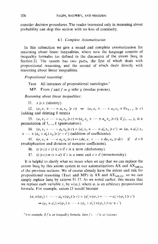
4.1. Complete Axiomatization
In this subsection we give a sound and complete axiomatization for reasoning about linear inequalities, where now the language consists of inequality formulas (as defined in the discussion of the axiom Ineq in Section2). The system has two parts, the first of which deals with propositional reasoning, and the second of which deals directly with reasoning about linear inequalities.
Propositional reasoning:
Taut. All instances of propositional tautologie~.~
MP. From f and f * g infer g (modus ponens).
Reasoning about linear inequalities:
11. x > x (identity).
12. ( a , x , + ... + a,x, 3 c) o ( a , x l + . . . + a,x, + Ox,,, 3 c) (adding and deleting 0 terms)
13. ( a , x , + ... +akxk3c)=>(a , ,x , ,+ ... +a,,x,,>c), i f j , , ..., jk is a permutation of 1, ..., k (permutation).
14. ( a , x ,+ . . . + a k x k > c ) ~ ( a ' , x l + . . . + a ;x ,3c f ) * ( a , + a ' , ) x , + . . . + (a, + a;) xk 3 (c + c') (addition of coefficients).
15. (a ,x , + . . . + akxk > c ) o (da ,x , + . - . + da,x, >dc) if d>O (multiplication and division of nonzero coefficients).
16. (t 3 c) v ( t Q c) if t is a term (dichotomy).
17. ( t 3 c) =. (t > d) if t is a term and c > d (monotonicity).
It is helpful to clarify what we mean when we say that we can replace the axiom Ineq by this axiom system in our axiomatizations AX and AXMEAs of the previous sections. We of course already have the axiom and rule for propositional reasoning (Taut and MP) in AX and AXMEAs, so we can simply replace Ineq by axioms 11-17, As we noted earlier, this means that we replace each variable x , by w(cp,), where cpi is an arbitrary propositional formula. For example, axiom I3 would become
For example, i f f is an inequality formula, then t v 7 f is a n instance.
LOGIC FOR REASONING ABOUT PROBABILITIES 107
We note also that I1 (which becomes w(q) 3 w(q)) is redundant in AX and AXMEAs, because it is a special case of axiom W4 (which says that w(cp) = w ( $ ) if cp i- $ is a propositional tautology).
We call the axiom system described above A X I N E Q . In this section, we show that AX,,,,, is sound and complete.
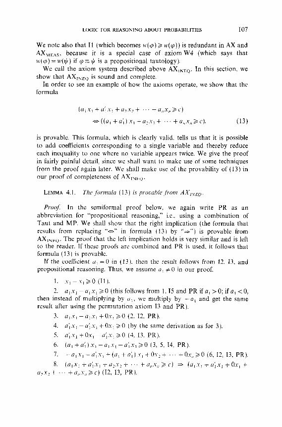
In order to see an example of how the axioms operate, we show that the formula
is provable. This formula, which is clearly valid, tells us that it is possible to add coefficients corresponding to a single variable and thereby reduce each inequality to one where no variable appears twice. We give the proof in fairly painful detail, since we shall want to make use of some techniques from the proof again later. We shall make use of the provability of (13) in our proof of completeness of AX,,,,.
LEMMA 4.1. The fornzula ( 1 3 ) is procahle from AX,,,,.
ProoJ: In the semiformal proof below, we again write PR as an abbreviation for "propositional reasoning," i.e., using a combination of Taut and MP. We shall show that the right implication (the formula that results from replacing "ow in formula ( 1 3 ) by "-") is provable from AX,,,,. The proof that the left implication holds is very similar and is left to the reader. If these proofs are combined and PR is used, it follows that formula ( 1 3 ) is provable.
If the coefficient 17, = 0 in (13) . then the result follows from 12, 13, and propositional reasoning. Thus, we assume a , # O in our proof.
I . x - . Y , 2 0 (11).
2. a , x , - u,.u, 3 0 (this follows from 1,15 and PR if a , > O ; if a , <0, then instead of multiplying by a , , we multiply by - a , and get the same result after using the permutation axiom I3 and PR) .
3. a , .u, - al.u, + O s , 3 0 (2 , 12, PR) .
4. a', .u, - a; s, + Or, 3 0 (by the same derivation as for 3). 5. a',.u, +Ox, - a ' , s l 3 0 (4, 13, PR) .
6. ( a , + a ; ) .u, - a , s , - a',.u,30 ( 3 , 5 , 14, PR) .
7 . - a l . u , - a ~ . u l + ( a , + a ~ ) r , + O ~ 2 + . . . + 0 . ~ , , > 0 ( 6 , 1 2 , 1 3 , PR) .
8. ( a , x , + a; .u, + o,.r2 + . . . + a, , .~ , , 3 r ) * ( a , .u, + a; .u, + Ox, + a2.u, + . . . + a,,r,, 3 c ) (12, I?, PR) .
108 FAGIN, HALPERN, AND MEGIDDO
9. ( a , x , +a',x, +Ox, + a 2 x 2 + ... +a,x,>c) A ( - a l x , -a ' ,x , + ( a , + a',) x 1 + Ox2 + ... + Ox, 3 0 ) (Ox, + Ox, + ( a , + a ; ) x , + a2x2 + .. . +u,x,>c) (14).
10. (Ox, +Oxl + (a , + a ; ) x l + a2x2 + . . . + a,x, 3 c ) ( ( a , + a; ) x , +a,x2+ . . . +a, ,x ,3c) (12, 13, PR).
11. ( a , x , +a',x, + a 2 x 2 + - t - t - t + a , , x n 3 c ) * ( ( a , + a ; ) x , +a2x2+ . . +a,,x,>c) (7, 8, 9, 10, PR). 1
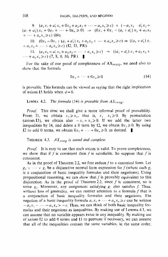
For the sake of our proof of completeness of AXINEQ, we need also to show that the formula
is provable. This formula can be viewed as saying that the right implication of axiom I 5 holds when d = 0.
LEMMA 4.2. The formula (14) is provable from AX,,,,.
Proof: This time we shall give a more informal proof of provability. From 11, we obtain x , 3 x l , that is, x , - x , 3 0 . By permutation (axiom I3), we obtain also -x, + x , 3 0. If we add the latter two inequalities by 14, and delete a 0 term by 12, we obtain Ox, 3 0. By using I2 to add 0 terms, we obtain Ox, + . . . + Ox,, 3 0, as desired. 1
THEOREM 4.3. AXlNEQ is sound and complete.
Proof: It is easy to see that each axiom is valid. To prove completeness, we show that iff is consistent then f is satisfiable. So suppose that f is consistent.
As in the proof of Theorem 2.2, we first reduce f to a canonical form. Let g , v . . . v g, be a disjunctive normal form expression for f (where each g, is a conjunction of basic inequality formulas and their negations). Using propositional reasoning, we can show that f is provably equivalent to this disjunction. As in the proof of Theorem 2.2, since f is consistent, so is some g,. Moreover, any assignment satisfying g , also satisfies f: Thus, without loss of generality, we can restrict attention to a formula f that is a conjunction of basic inequality formulas and their negations. The negation of a basic inequality formula a , x, + . . , + a,x, c can be written - a , x , - . . . -a,x, > -c. Thus, we can think of both basic inequality for- mulas and their negations as inequalities. By making use of Lemma 4.1, we can assume that no variable appears twice in any inequality. By making use of axiom I2 to add 0 terms and I3 to permute if necessary, we can assume that all of the inequalities contain the same variables, in the same order,
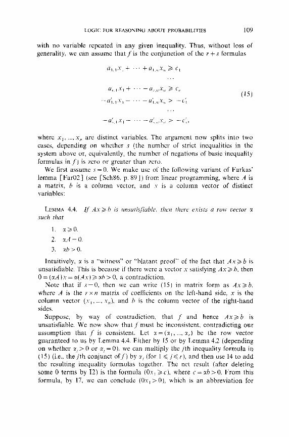
LOGIC FOR REASONING ABOUT PROBABILITIES 109
with no variable repeated in any given inequality. Thus, without loss of generality, we can assume that f is the conjunction of the r + s formulas
a , , , x , + . . . +a,. ,,,. u,, 3 c,.
- a ; , , x l - . . . -a;,,,x,, > -c',
where x , , ..., x , are distinct variables. The argument now splits into two cases, depending on whether s (the number of strict inequalities in the system above or, equivalently, the number of negations of basic inequality formulas in f ) is zero or greater than zero.
We first assume s = 0. We make use of the following variant of Farkas' lemma [Far021 (see [Sch86, p. 891) from linear programming, where A is a matrix, h is a column vector, and s is a column vector of distinct variables:
LEMMA 4.4. If A.u 3 h is unsutisfiable, then there exists a row vector cx such that
Intuitively, r is a "witness" or "blatant proof" of the fact that A x 3 b is unsatisfiable. This is because if there were a vector .u satisfying A x 3 h, then 0 = ( c t A ) . ~ = r(A.u) 2 rh > 0, a contradiction.
Note that if s = 0, then we can write (15) in matrix form as A x 3 b, where A is the r x n matrix of coefficients on the left-hand side, x is the column vector (s,, ..., x,,), and b is the column vector of the right-hand sides.
Suppose, by way of contradiction, that f' and hence A x > b is unsatisfiable. We now show that f must be inconsistent, contradicting our assumption that f is consistent. Let r = ( r , , ..., x,.) be the row vector guaranteed to us by Lemma 4.4. Either by I5 or by Lemma 4.2 (depending on whether a, > O or 2, = 0), we can multiply the j th inequality formula in (15) (i.e., the j th conjunct o f f ) by r , (for 1 < j $ r ) , and then use I4 to add the resulting inequality formulas together. The net result (after deleting some 0 terms by 12) is the formula (O.u, 2 c), where c = rh > 0. From this formula, by 17, we can conclude (Ox, > 0 ) , which is an abbreviation for
110 FAGIN, HALPERN, AND MEGIDDO
i (Ox, 6 O ) , which is in turn an abbreviation for i ( -Ox, 3 -0) , i.e., i ((Ox, 3 0) . Thus f - i (Ox, 3 0 ) is provable.
However, by Lemma 4.2, (Ox, 2 0 ) is also provable. It follows by propositional reasoning that if is provable, that is, f is inconsistent. Thus the assumption that f is unsatisfiable leads to the conclusion that f is incon- sistent, a contradiction.
We now consider the case where s > 0. Farkas' lemma does not apply, but a variant of it, called Motzkin's transposition theorem, which is due to Fourier CFou261, Kuhn CKuh561, and Motzkin [Mot561 (see [Sch86, p. 94]), does. A and A' are matrices, b and b' are column vectors, and x is a column vector of distinct variables.
LEMMA 4.5. If the system Ax 3 b, A'x > b' is unsatis$able, then there exist row vectors a, a' such that
1. a 3 0 a n d a ' 3 0 .
2. rxA + a'A' = 0.
3. Either
(a) ab + a'b' > 0, or
(b) some entry of a' is strictly positive, and ab + a'b' 2 0.
We now show that a and rx' together form a witness to the fact that the system A x 3 6, A'x > b' is unsatisfiable. Assume that there were x satisfying Ax 3 b and A'x > b'. In case 3(a) of Lemma 4.5 (ab + a'b' > 0 ) , we are in precisely the same situation as that in Farkas' lemma, and the argument after Lemma 4.4 applies. In case 3(b ) of Lemma 4.5, let A = ( A ' x ) - b'; thus, A is a column vector and A > 0. Then O = (aA + sc1A')x= ( c A ) x + ( a ' A f ) x = % ( A x ) + al (A 'x ) 3 ab + a'(bJ + A ) = (ab + a'b') + a'A 3 r'A > 0, where the last inequality holds since every a; is nonnegative, some a: is strictly positive, and every entry of A is strictly positive. This is a contradiction.
In order to apply Motzkin's transposition theorem, we write (15) as two matrix inequalities: Ax 3 b, where A is the r x n matrix of coefficients on the left-hand side of the first r inequalities (those involving "a") , x is the column vector (x , , ..., x,), and b is the column vector of the right-hand sides of the first r inequalities; and A'x > b', where A' is the s x n matrix of coefficients on the left-hand side of the last s inequalities (those involving ">"), and b' is the column vector of the right-hand sides of the last s inequalities.
Again assume that f is unsatisfiable. Let a= ( a , , ..., a,) and r ' = ( a ; , ..., a:) be the row vectors guaranteed to us by Lemma 4.5. In case 3(a) of Lemma 4.5, we replace every ">" in (15) by "3" and proceed to derive
LOGIC FOR REASONING ABOUT PROBABILITIES 111
a contradiction as in the case s = 0. Note that we can do this replacement by 16, since t > c is an abbreviation for i ( t < c).
In order to deal with case 3 (b ) of Lemma 4.5, we need one preliminary lemma, which shows that a variation of axiom I5 holds.
LEMMA 4.6. ( a , x , + . . . + a , s , > c ) o ( d a , , ~ , + . . .+ du,.u,>dc) is provable, if' d > 0.
Proof. The formula
is an instance of axiom 15. By taking the contrapositive and using the fact that t > c is an abbreviation for i ( - t 3 - c) , we see that the desired formula is provable. 4
Since we are considering case 3 (b) of Lemma 4.5, we know that some a; is strictly positive: without loss of generality, assume that x: is strictly positive. For 1 6 j < s - 1, let us replace the " >" in the j th inequality involving ">" in (15) by "3." Again. this is legal by 16. As before, either by axiom 15 or by Lemma 4.2, we can multiply the jth inequality formula in the system (1 5 ) by a, (for 1 < j < r ) , and multiply each of the next s - 1 inequalities that result when we replace > by 2 by r j , j= 1, ..., s - 1, respectively. Finally, by Lemma 4.6. we can multiply the last inequality in (15) by a, (which is strictly positive, by assumption). This results in the system of inequalities
r,.a , , . Y , + . . . +x,.u ,.,, s,, 3 r,c,
Let us denote the last inequality (the inequality involving ">") in (16) by g. Let a j'x, + . . . + a , ~ s , , 3 d be the result of "adding" all the inequalities in (16) except g. This inequality is provable from f using 14. Since xA + x'A' = 0, we must have that r',a: , = a;', for j = 1, ..., n. So the inequality g is ( -a;',u, - . . . - a,:j.u,, > - r : c: ). Since r b + r'h' > 0, it follows that - sc: c: 3 - d. Hence. the formula g - ( - a;'u, - . . . - a,y.u,, > - d ) is
112 FAGIN, HALPERN, AND MEGIDDO
provable using I7 and propositional reasoning (there are two cases, depending on whether -a:c: = - d or -a:c.:. > - d ) . Now -a;'x, - ... - a:x, > -d is equivalent to a;x , + . . . + a:x, < d. But this contradicts a;'x, + . . . + a i x , 2 d, which we already showed is provable from f: It follows by propositional reasoning that i f is provable, that is, f is inconsistent, as desired.
Since we have shown that assuming f is unsatisfiable leads to the conclu- sion that f is inconsistent, it follows that if f is consistent then f is satisfiable. I
4.2. Small-Model Theorem
A "model" for an inequality formula is simply an assignment to variables. We think of an assignment to variables as "small" if it assigns a nonzero value to only a small number of variables. We now show that a satisfiable formula is satisfiable by a small assignment to variables.
As we did with weight formulas, let us define the length If 1 of an inequality formula f to be the number of symbols required to writef, where we count the length of each coefficient as 1. We have the following "small-model theorem."
THEOREM 4.7. Suppose f is a satisfiable inequality formula. Then f is satisfied by an assignment to variables where at most 1 f 1 variables are assigned a nonzero value.
Proof: As in the completeness proof, we can write f in disjunctive normal form. It is easy to show that each disjunct is a conjunction of at most I f 1 basic inequality formulas and their negations. Clearly, since f is satisfiable, one of the disjuncts is satisfiable. The result then follows from Lemma 4.8, below, which is closely related to Lemma 2.5. Lemma 2.5 says that if a system of r linear equalities and/or inequalities has a nonnegative solution, then it has a nonnegative solution with at most r entries positive. Lemma4.8, by contrast, says that if the system has a solution (not necessarily nonnegative), then there is a solution with at most r variables assigned a nonzero (not necessarily positive) value.
LEMMA 4.8. If a system of r linear equalities andlor inequalities has a solution, then it has a solution with at most r variables assigned a nonzero value.
Proof: By the comment after Lemma 2.5, we can pass to a system of equalities only.
Hence, let A x = b represent a satisfiable system of linear equalities, where A has r rows; we must show that there is a solution where at most r of the
L.OGIC FOR REASONING ABOUT PROBABILITIES 113
variables are assigned a nonzero value. Since A x = b is satisfiable, it follows that b is in the vector space V spanned by the columns of A. Since each column is of length r, it follows from standard results of linear algebra that V is spanned by some subset of at most r columns of A. So b is the linear combination of at most r columns of A. Thus, there is a vector y* with at most r nonzero entries, where Ay* = b. This proves the lemma. 1
4.3. Decision Procedure
As before, when we consider decision procedures, we must take into account the length of coefficients. Again, we define / f 1 1 to be the length of the longest coefficient appearing inf , when written in binary, and we define the size of a rational number alb, where a and h are relatively prime, to be the sum of lengths of a and h, when written in binary. We can then extend the small-model theorem above as follows:
THEOREM 4.9. Suppose f is a sutisji'able inequali!,, formula. Then f is satisfied by an assignment to cariables nhere at most I f 1 variables are assigned a nonzero value and nhere the calue assigned to each variable is a rational number with size O( I f 1 I f l l + If l log( I f 1 ) ) .
Theorem 4.9 follows from the proof of Theorem 4.7 and the following simple variation of Lemma 4.8, which can be proven using Cramer's rule and simple estimates on the size of the determinant.
LEMMA 4.10. Zf a sj,stenz of r. linear equalities and/or inequalities with integer coefficients each of length at most 1 has a solution, then it has a solution with at most r. cariables assigned a nonzero calue and where the size of each member of the solution is O(r l+ r. log(r)).
As a result, we get
THEOREM 4.1 1. The probleni of' deciding ~vherher an inequality formula is satisfiable in a measurable probabilitj, structure is NP-complete.
Proof For the lower bound, a propositional formula cp is satisfiable iff the inequality formula that is the result of replacing each propositional variable pi by the inequality s, 3 0 is satisfiable. For the upper bound, given an inequality formula,f, we guess a satisfying assignment to variables for f with at most 1 f 1 variables being assigned a nonzero value such that each nonzero value assigned to a variable is a rational number with size O(l f 1 11 f 11 + 1 f 1 log(1 f I)). We then verify that the assignment satisfies the inequality formula. I

114 FAGIN, HALPERN, AND MEGIDDO
We now turn our attention to reasoning about conditional probability. As we pointed out in the Introduction, the language we have been con- sidering is not sufficiently expressive to allow us to express statements such as 2w(p2 I p i ) + w(p, j p,) 2 1. Suppose we extend our language to allow products of terms, so that formulas such as 2w(p,) w(p2) >, 1 are allowed. We call such formulas polynomial weight formulas. To help make the con- trast clearer, let us now refer to the formulas we have been calling "weight formulas" as "linear weight formulas." We leave it to the reader to provide a formal syntax for polynomial weight formulas. Note that by clearing the denominators, we can rewrite the formula involving conditional probabilities to 2w(p, A p2) w(p2) + 2 ~ 4 p , A p,) w(p,) 2 w(p,) w(p2), which is a polynomial weight f o r m ~ l a . ~
In order to discuss decision procedures and axiomatizations for polyno- mial weight formulas, we need to consider the theory of real closed fields. We now define a real closed field. All of our definitions are fairly standard (see, for example, [Sho67]). An ordered field is a field with a linear ordering < , where the field operations + (plus) and . (times) respect the ordering: that is, (1) x < y implies that x + z < y + z , and (2) if x and y are positive, then so is x . y. A real closedfield is an ordered field where every positive element has a square root and every polynomial of odd degree has a root. Tarski showed [Tar51, Sho671 that the theory of real closed fields coincides with the theory of the reals (under +, ., < and constants 0, 1, -1). That is, any first-order formula that involves only +, ., < ,0 , 1, - 1 is true about the real numbers if and only if it is true of every real closed field.
Tarski [Tar511 showed that the decision problem for this theory is decidable. Ben-Or, Kozen, and Reif [BKR86] have shown that the deci- sion problem is decidable in exponential space. Fischer and Rabin [FR74] prove a nondeterministic exponential time lower bound for the complexity of the decision problem. In fact, Fischer and Rabin's lower bound holds even if the only nonlogical symbol is + (plus). Berman [BerFIO] gives a slightly sharper lower bound in terms of alternation. Canny [Can881 has shown recently that the quantifier-free fragment is decidable in polynomial space.
We do not know a sound and complete axiomatization for polynomial weight formulas. For this reason, later we shall allow first-order quantifica- tion, which will enable us to obtain a complete axiomatization in a larger
'Actually, it might be better to express it as the polynomial weight formula w ( p , ) f O A
w ( p 2 ) ZO = ( 2 1 . 4 ~ ~ A p 2 ) w ( p 2 ) + 2 w ( p 1 A p 2 ) ~ ( p , ) 2 w ( p I ) w ( p 2 ) ) , to take care of the case where the denominator is 0.
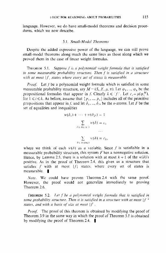
LOGIC FOR REASONING ABOUT PROBABILITIES 115
language. However, we do have small-model theorems and decision proce- dures, which we now describe.
5.1. Small-Model Theorems
Despite the added expressive power of the language, we can still prove small-model theorems along much the same lines as those along which we proved them in the case of linear weight formulas.
THEOREM 5.1. Suppo~e f is a polynomial weight formula that is satisfied in some measurable probability structure. Then f is satisfied in a structure uYth at most 1 f 1 states where ecery set of states is measurable.
Proof. Let f be a polynomial weight formula which is satisfied in some measurable probability structure, say M = ( S , X, p, rr). Let q , , ..., 47, be the propositional formulas that appear in J: Clearly k 6 I ( f 1 1 . Let c, = p(cp;n"), for 1 6 i d k. As before, assume that { p , , ..., p,,) includes all of the primitive propositions that appear in j; and let d , , ..., dl,, be the n-atoms. Let F be the set of equalities and inequalities
where we think of each I I . ( ~ ) as a variable. Since f is satisfiable in a measurable probability structure, this system F has a nonnegative solution. Hence, by Lemma 2.5, there is a solution with at most k + 1 of the ~ ( 6 ) ' s positive. As in the proof of Theorem 2.4, this gives us a structure that satisfies f with at most I f 1 states, where every set of states is measurable.
Note. We could have proven Theorem 2.4 with the same proof. However, the proof would not generalize immediately to proving Theorem 2.6.
THEOREM 5.2. Let f be a pol~womial ,!,eight formula that is satisfied in some probability structure. Then it is satisfied in a structure ~vith at most 1 f l 2 states, and with a basis of size at most I f l .
Prooj: The proof of this theorem is obtained by modifying the proof of Theorem 3.9 in the same way in which the proof of Theorem 5.1 is obtained by modifying the proof of Theorem 2.4. 1
116 FAGIN, HALPERN, AND MEGIDDO
5.2. Decision Procedures
In Sections 2 and 3, we were able to obtain decision procedures for linear weight formulas by extending the small-model theorems to show that not only are there small models, but there are small models where the probabilities have a "small" length. Such a result is false for polynomial weight formulas (consider 2w(p) w(p)= 1). Hence, in order to obtain a decision procedure in this case, we use a different technique for deciding satisfiability: We reduce the problem to a problem in the quantifier-free theory of real closed fields and then apply Canny's decision procedure.
THEOREM 5.3. There is a procedure that runs in polynomial space for deciding if a polynomial weight formula is satisfiable in a measurable probability structure.
Proof: Let f be a polynomial weight formula, where the distinct primitive propositions that appear in f are p, , ..., p,. Let 6,, ..., 6 p be the n-atoms, and let T be a subset of the n-atoms, with at most I f 1 members. Assume that the members of T are precisely ai,, ..., a,,, where i, < . . . < i,. Let x , , ..., x, be variables (as many variables as the cardinality of T), where intuitively, x, will correspond to w(6,,)). Let ,f, be the conjunction of x, + ... + x, = 1 with the result of replacing each term w(q) of f by C61JEAfn(W, xi. By Theorem 5.1, it is easy to see that f is satisfiable in a measurable probability structure iff for some T with at most 1 f 1 members, f, is satisfiable over the real numbers (that is, iff there are real numbers x,*, ..., x: such that the result of replacing each variable xi by x* is true about the real numbers). It is straightforward to verify that I f,l is polyno- mial in I f 1, where I f , l is the length off,, and again we count the length of each coefficient as 1.
We would now like to apply Canny's decision procedure for checking if f T is satisfiable, but there is one small problem. The formula f T has arbitrary integer coefficients, whereas the language of real closed fields allows only the constants 0, 1, and - 1. Now we could replace a constant like 17 by 1 + ... + 1 (17 times). This would result in a formula f ', that is in the language of real closed fields, but I f might be exponential in 1 1 f 1 1 . The solution is to express 17 as 24 + 1 and then write this in the language of real closed fields as ( 1 + 1 ) ~ ( 1 + 1 ) ~ ( 1 + 1 ) ~ ( 1 + 1 ) + 1 . Using this technique we can clearly represent any coefficient whose length is k when written in binary by an expression in the language of real closed fields of length 0 ( k 2 ) . Let f; be the formula that results by representing the coefficients off, in this way. Thus I f ',I is polynomial in I f 1 . I f 1 1 .
The PSPACE decision procedure for satisfiability of f proceeds by systematically cycling through each candidate for T and using Canny's PSPACE algorithm to decide iff > is satisfiable over the real numbers. Our

LOGIC FOR REASONING ABOUT PROBABILITIES 117
algorithm says that f is satisfiable iff f > is satisfiable over the real numbers for some T. I
THEOREM 5.4. There is a procedure that runs in polynomial space for deciding whether a polynomial tceight ,formula is satisfiable in a (general) probability structure.
Proof: Let f be a polynomial weight formula. Assume that { y , , ..., p,,) includes all of the primitive propositions that appear in J Define a partial probability structure to be a tuple Q = (S, B, n), where S is a set (thought of as a set of states); B = { T , , ..., T, } gives a partition of S, that is, the T,'s are nonempty and pairwise disjoint, and their union is S (we think of B as being a basis); and ~ ( s ) is a truth assignment for every state in S, where we assume that n( .~)(p) =false for every primitive proposition p that does not appear in f (note: the analog to Lemma 2.8 holds, so we do not care about primitive propositions that do not appear in f ). Intuitively, a partial probability structure gives all the information about a probability structure except the measure of the basis elements. For each propositional formula cp over { p , , ..., p,,), define V(q) c (1, ..., t ) by letting i~ V(cp) iff cp is true under the truth assignment ~ ( b ) for every h E T,. Intuitively, if we expanded Q to a probability structure M by defining the measure of each basis element, then the inner measure of cp would be obtained by adding the measures of each T,, where i~ V(q). Let .u,, ..., .u, be variables (as many variables as the cardinality of B), where intuitively, .u, corresponds to the measure of T,. Let , fQ be the conjunction of .u, + . . . + x, = 1 with the result of replacing each term t t fcp) off by E l E ,.,w, .u, (and by 0 if V(q) is empty) and replacing each integer coefficient off by the appropriate representation as discussed in the proof of Theorem 5.3. By Theorem 5.2, it is easy to see that f is satisfiable in a probability structure iff for some "small" partial probability structure Q (that is, a partial probability structure Q = ( S , B, n), where S has at most I f l h e m b e r s and B has at most If 1 mem- bers), ,fQ is satisfiable over the real numbers. It is easy to see that if Q is small, then the size of,fQ is polynomial in If 1 . 1 1 f 11. The PSPACE decision procedure for satisfiability o f f proceeds by systematically cycling through each small partial probability structure Q, and using Canny's PSPACE algorithm to decide if,fQ is satisfiable over the real numbers. Our algorithm says that f is satisfiable iff one of these ,fQ's is satisfiable over the real numbers. 1
The basic idea in proving completeness for linear weight formulas was to use the axioms WlLW4 to reduce the problem to checking validity of a set
118 FAGIN, HALPERN, AND MEGIDDO
of linear inequalities and then apply the axiom Ineq. In the case of polyno- mial weight formulas we want to use a similar technique. In this case, we use W1-W4 to reduce the problem to checking validity of a formula in the language of real closed fields and then apply a sound and complete axiomatization for real closed fields. There is only one difficulty in carrying out this program: the theory of real closed fields allows first-order quan- tification over the reals. Thus, in order to carry out our program, we must extend the language yet again to allow such quantification.
We define a basic,first-order weight formula to be like a basic polynomial weight formula, except that now we allow variables (intended to range over the reals) in expressions. Thus, a typical basic first-order weight formula is
The set of first-order weight formulas is obtained by closing off the basic first-order weight formulas under conjunction, negation, and first-order quantification (where the quantification is over the reals). In order to ascribe semantics to first-order weight formulas, we now need a pair con- sisting of a probability structure M and a valuation v, where a valuation is a function from variables to the reals that gives meaning to the free variables in the formula. Thus, for example, if M = ( S , %, p, n), then
We deal with quantification as usual, so that (M, v ) k Vxcp iff (M, v ' ) + cp for all v' that agree with v except possibly in the value that they assign to x. We leave the remaining details to the reader. It would be quite natural to restrict attention to sentences, i.e., formulas with no free variables. Note that the truth or falsity of a sentence is independent of the valuation. We shall usually not bother to do so. Thus, when we say that a first-order weight formula is satisfiable, we mean that there is a probability structure M and a valuation v such that (M, v ) f: Note that a formula f with free variables x,, ..., x, is satisfiable iff the sentence 3x, . . . 3x, f is satisfiable. Similarly, f is valid iff the sentence Qx, . . . Qx, f is valid.
We can prove a small-model theorem for first-order weight formulas using techniques identical to those used in Theorems 5.1 and 5.2.
THEOREM 6.1. Let f be a first-order weight formula that is satisfied in some measurable probability structure. Then f is satisfied in a structure with at most I f 1 states where every set of states is measurable.
LOGIC FOR REASONING ABOUT PROBABILITIES 119
THEOREM 6.2. Let f be a first-order weight formula that is satisfied in some probability structure. Then f is satisfied in a structuw with at most 1 f 1 states, and with a basis of size at most I f 1 .
We can also obtain decision procedures for first-order weight formulas by appropriately modifying Theorems 5.3 and 5.4, except that instead of using Canny's PSPACE algorithm, we use Ben-Or, Kozen, and Reif's exponential space algorithm (since the first-order formulas f ; and fQ of the proofs are no longer necessarily quantifier-free).
THEOREM 6.3. There is a procedure that runs in exponential space for deciding whether a first-order ]$>eight formula is satisfiable in a measurable probability structure.
THEOREM 6.4. There is a procedure that runs in exponential space for deciding whether a first-order rreight formula is satisfiable in a (general) probability structure.
In order to get a complete axiomatization for first-order weight formulas, we begin by giving a sound and complete axiomatization for real closed fields, which Tarski [Tar511 proved is complete for the reals. The version we give is a minor modification of that appearing in [Sho67]. The non- logical symbols are t , ., < , 0, 1, - 1.
First-order reasoning:
FO-Taut. All instances of valid formulas of first-order logic with equality (see, for example, [End72, Sho671).
MP. From f and j'* g infer g (modus ponens).
Reasoning about real closed fielrls:
V x VJ' V z ( ( s + J ! ) + z = s + ( j ' t z ) ) .
V.Y(.Y + 0 = s).
Vx( .u+(-1 . x ) = O ) .
V.Y VJ'(.Y + J' = j' + s). v x v y VZ(( .Y . 1.) . z = x . ( j . . ,)).
V.Y(.Y . 1 = x). V x ( x # O * 3 y ( . u . y = 1 ) ) .
V.Y V y ( u . y = J' . .Y).
V.Y v y Vz(.u. ( j , + s) = (s . y ) t (s .:I). O f 1.
V X ( 1 ( Y < Y ) ) .
120 FAGIN, HALPERN, AND MEGIDDO
F12. Vx Vy Vz((x < y ) A ( y < z ) * (x < z ) ) .
F13. VxVy( (x<y)v ( x = y ) v ( y < x ) ) .
F14. Vx Vy Vz((x < y ) * ( (x + z ) < ( y + z))).
F15. V x V y ( ( ( O < x ) ~ ( O < y ) ) * ( O < x ~ y ) ) .
F16. Vx((0 < x) 3 3y(y. y = x)).
F17. Every polynomial of odd degree has a root.
An instance of axiom F17, which would say that every polynomial of degree 3 has a root, would be
Axioms F1-F10 are the field axioms, axioms F11-F13 are the axioms for linear orders, axioms F14-F15 are the additional axioms for ordered fields, and axioms F16-F17 are the additional axioms for real closed fields. Let us denote the axiom system above by AXRcF. Then AXRcF is a sound and complete axiomatization for real closed fields CTar51, Sho671. Let us denote by the result of taking AXRcF along with our axioms WlLW4 and one more axiom, F18, below, that lets us replace the integer coefficients that appear in weight formulas by an expression in the language of real closed fields:
F18. k = 1 + ... + 1 (k times).
(We remark that there is no need to use an efficient representation of integer coefficients here, as there was, say, in Theorem 5.3, since complexity issues do not arise.) Let us denote by AX,, the result of replacing W3 in AX ,,~,,,, by W5 and W6.' We now show that is a sound and complete axiomatization for first-order weight formulas with respect to measurable probability structures, and AXFo is a sound and complete axiomatization for first-order weight formulas with respect to (general) probability structures.
THEOREM 6.5. AX,,.,,,, is a sound and complete axiomatization for first-order bveight formulas with respect to measurable probability structures.
Proof: From what we have said, it is clear that AX,,.,,,, is sound. To show completeness, we carry out the ideas sketched at the beginning of this section: namely, we reduce a first-order weight formula to an equivalent formula in the language of real closed fields. Assume that f is a first-order weight formula that is unsatisfiable with respect to measurable probability structures (that is, there is no measurable probability structure that satisfies
'The occurrences of 3 is an expression such as 1 , 2 1, in WlLW6 can be viewed as an abbreviation for ( r I < r , ) v ( r , = r z ) , which is a formula in the language of real closed fields.
LOGIC FOR REASONING ABOUT PROBABILITIES 121
it). Let p,, ..., p,, include all of the primitive propositions that appear in ,f; and let 6,, ..., 6," be the n-atoms. Let x,, ..., x,, be new variables, where intuitively, xi represents w(6 , ) . Let f ' be 3x, . . . 3 ~ , , ~ g , where g is the conjunction of
along with the result of replacing each 1 2 j c p ) in f by Ed,,, x, (and by 0 if cp is equivalent to false) and replacing each integer coefficient k in f by 1 + . . . + 1 (k times). It is easy to see that since f is unsatisfiable with respect to measurable probability structures, it follows that f ' is false about the real numbers. By Tarski's result on the completeness of AXRcF, it follows that if ' is provable in AXRcF. By making use of Lemma 2.3 (which again holds, by essentially the same proof), it is not hard to see that i f is provable in AX,,.,,,,. The straightforward details are omitted. 1
To prove completeness of AX,, in the general (nonmeasurable) case, we need a lemma, which is completely analogous to Theorem 3.7. Let f be a first-order weight formula, where ( p i , ..., p,, ] includes all of the primitive propositions that appear in f , and let p , , ..., p p be the n-regions. Let x,, ..., x22" be new variables (one new variable for each n-region), where intuitively, x, corresponds to ~ ( p , ) . Let ,?be the result of replacing each w(p) in f by x,, where p, is the n-region equivalent to p. Let 7 be ,f A (xi = 0) A (.u,?l~ = 1 ) A "N.u 3 0," where "Ns 2 0 is the conjunction of the inequalities N.u 2 0.
LEMMA 6.6. Let f be a first-order weight formula. Then f is satisfied in some prohabilitjt structurcJ jff.7 is satisfiable over the real numhers.
Proof: The proof is virtually identical to that of Theorem 3.7. For example, if.Tis satisfiable over the real numbers, then let .x" = x:, ..., x$n be real numbers such that the result of replacing each .Y, in f: by .u: is true about the real numbers. The proof of Theorem 3.7 shows how to use x* to build a probability structure that satisfies f.
THEOREM 6.7. A X F , is a sound and complete uxiomutixtion ,for ,first- order weight formulas with respect to (generul) probability structures.
Proof: Again, it is clear that AX, ,, is sound. To show completeness, assume thatf is an unsatisfiable first-order weight formula (that is, there is no probability structure that satisfies i t ) . Lct 1' bc 3.u, . . . 3 . ~ ~ 2 1 3 7 By
122 FAGIN, HALPERN, AND MEGIDDO
Lemma 6.6, f ' is false about the real numbers. By Tarski's result again on the completeness of AX,,,, it follows that i f ' is provable in AXRcF. As before, it is therefore not hard to see that if is provable in AXFo. Again, the straightforward details are omitted. I
We close this section with a few remarks on how these results relate to those obtained in [Bac88] and [AH89, Ha1891. In Bacchus' language it is possible to represent probabilities of first-order formulas. However, while we place probabilities on possible worlds here, Bacchus instead places the probability on the domain. Thus (using our notation), he would allow a formula such as Vx(w, (P(x , y)) 2 f ) , which should be read "for all x, the probability that a random y satisfies P(x , y) is at least f ." In addition, first- order quantification over probabilities is allowed, as in a formula of the form 3r Vy(w,.(P(x, y)) 2 r). Thus we can view Bacchus' language as an extension of first-order weight formulas, where the arguments of the weight function are first-order formulas rather than just propositional formulas. There is an additional technical difference between our approach and that of Bacchus. Bacchus' "probabilities" do not have to be real valued; they can take values in arbitrary ordered fields. Moreover, Bacchus requires his probability measures to be only finitely additive rather than countably additive; thus they are not true probability measures. Bacchus does provide a complete axiomatization for his language. However, a formula that is valid when the probabilities take on real values is not necessarily provable in his system, since it may not be valid when probabilities are allowed to take values in arbitrary ordered fields. On the other hand, Bacchus' axioms are all sound when probability is interpreted in the more standard way and, as Bacchus shows, they do enable us to prove many facts of interest regarding the probability of first-order sentences.
More recently, in CHa1891, two first-order logics of probability are presented. One, in the spirit of Bacchus, puts probability on the domain while the other, more in the spirit of our approach here, puts probability on the possible worlds. It is shown that these ideas can be combined to allow a logic where we can reason simultaneously about probabilities on the domain and on possible worlds. In all cases, the probabilities are countably additive and take values in the reals. In [AH891 it is shown that in general the decision problem for these logics is wildly undecidable (technically, it is ZZ:-complete). However, in some special cases, the logic is decidable; complete axiomatization for these cases are provided in [Ha189].
LOGIC FOR REASONING ABOUT PROBABILITIES 123
The Dempster-Shafer theory of evidence [Sha76] provides one approach to attaching likelihoods to events. This theory starts out with a belief function (sometimes called a support function). For every event A , the belief in A, denoted Bel(A), is a number in the interval [0, 11 that places a lower bound on likelyhood of A. Shafer [Sha76] defines a belief function (over S) to be a function Bel: 2' + [0, 1 ] (where, as usual, 2.' is the set of subsets of S) that satisfies the following conditions:
Property B3 may seem unmotivated. Perhaps the best way to understand it is as an analogue to the usual inclusion-exclusion rule for probabilities [Fe157, p. 891, which is obtained by replacing the inequality by equality (and the belief function Be1 by a probability function p). In particular, B3 holds for probability functions. In [FH89] it is shown to hold for all inner measures induced by probability functions. Thus, every inner measure is a belief function. The converse is almost true, but not quite. It turns out that roughly speaking, the converse would be true if the domain of belief functions and inner measures were formulas, rather than sets. We now give a precise version of this informal statement.
By analogy with probability structures, let us define a DS structure (where, of course, "DS" stands for Dempster-Shafer) to be a tuple D = ( S , Be/, x), where Be1 is a belief function over S, and as before, x associates with each state in S a truth assignment on the primitive propositions in @. For each propositional formula cp, we define c p D just as we defined cpM for probability structures M. Let M = (S, 3, p, x ) be a probability structure. Following [FH89], we say that D and M are equivalent if Bel(cpD) = p,(cpM) for every propositional formula cp.
For the purposes of the next theorem, we wish to consider probability structures and DS structures where there are effectively only a finite number of propositional variables. Let us say that a probability structure M = (S, X, p, x ) or a DS structure D = (S, Be/, x) is special if x(s)(p) = false for all but finitely many primitive propositions p and for every state s.
THEOREM 7.1 [FH89]. 1 . For rcerj-). special probability structure there is an equivalent special DS structure.
2. For every special DS structure there is an equivalent special probability structure.

124 FAGIN, HALPERN, AND MEGIDDO
It follows immediately that AX is a sound and complete axiomatization for linear weight formulas with respect to DS structures (i.e., where w(q) is interpreted as the belief in q).' Similarly, AX,, is a sound and complete axiomatization for first-order weight formulas with respect to DS struc- tures. All of our decision procedures carry over immediately. Thus, for linear weight formulas, the complexity of the decision problem with respect to DS structures is NP-complete; for polynomial weight formulas, there is a polynomial space procedure for deciding satisfiability (and validity), and for first-order weight formulas, there is an exponential space procedure for deciding satisfiability (and validity). Let W6' be the following axiom, which is obtained directly from Shafer's condition B3, above, in the obvious way.
In the remainder of this section, we show that we could just as well have used W6' as W6 throughout this paper. Let AX' (respectively, AX;,) be the axiom system that results when we replace W6 in AX (respectively, AX,,) by W6'.
THEOREM 7.2. The axiom system A X (respectively, A X F o ) is equivalent to the axiom system A X ' (respectively, AX;,).
Proof. For convenience, we restrict attention to AX, since the proof is essentially identical in the case of AX,,. We first show that i f f is an instance of axiom W6', then f is provable in AX. Assume not. Then -~ f is consistent with AX. By completeness (Theorem 3.8), there is a probability structure that satisfies ~ f . So by Theorem 7.1, there is a DS structure that satisfies iJ: However, this is impossible, since it is easy to see that every DS structure satisfies every instance of axiom W6'.
Now let f be an instance of axiom W6; we must show that f is provable in AX'. Let f be
C ( - l ) r - r w(pf) 2 0 , t = 1 p' a size t subregion of p
(18)
where p is the size r region 6, v . . . v S,, and r > 1. If r = 1, then (18) says w(SI) 2 0 , which is a special case of axiom W1. Assume now that r 2 2.
We can restrict attention to special structures because of Lemma 2.8, which implies that if we are concerned with the validity of a formulaf, then we can restrict attention without loss of generality to the finitely many primitive propositions that appear in f : In [FH89], attention was restricted to structures where there are only a finite numbers of primitive propositions, which is equivalent to considering special structures.
LOGIC FOR REASONING ABOUT PROBABILITIES 125
Define cp , , for 1 < i < r, to be the disjunction of each of a , , ..., 6 , except 6 , . Rewrite W6' as
We now show that ( 1 8 ) and ( 1 9 ) are equal, term by term. First, the w ( 6 , v . . . v c p , ) term of ( 1 9 ) is equal to w ( p ) , since c p , v ... v cp, is equivalent to p. This corresponds to the term of ( l a ) , where t = r and p' = p. Now consider the term of ( 1 9 ) , where the distinct members of I are precisely i,, ..., i,. It is straightforward to verify that A, c p i is equivalent to the t-subregion p' of p which is the disjunction of each of a , , ..., 6,. except 6 , . 6 where t = r - s. So the term ( - 1 ) " w ( A i G l c p , ) equals ( - 1)" w ( p f ) , which equals ( - w ( p l ) , a term of ( 1 8 ) . The only term of ( 1 9 ) that does not match up with a term of ( 1 8 ) occurs when I = (1, ..., r}; but then AiG, cp, is equivalent to false, so M . ( A , ~ , c p i ) = 0. Otherwise, there is a perfect matching between the terms of ( 1 8 ) and ( 1 9 ) . It follows easily that ( 1 8 ) is provable in AX'. 1
We have investigated a logic for reasoning about probability, both for cases where propositions necessarily represent measurable sets and for the general case. We have provided complete axiomatizations and decision procedures for a number of variants of the logic.
We were surprised both to be able to get fairly elegant complete axiomatizations for so rich a logic and to be able to prove that the satisfiability problem for the linear case is in NP. This is certainly the best we could have hoped for, since clearly the satisfiability problem for our logic is at least as hard as that of propositional logic. We remark that in [ G K P 8 8 , K a v 8 8 1 there is some discussion of subcases of the decision procedure for the measurable case that can be handled efficiently. It would be of interest to have further results on easily decidable subcases of the logic, or on good heuristics for checking validity.
While the focus of this paper is on technical issues-axiomatizations and decision procedures-it is part of a more general effort to understand reasoning about knowledge and probability. In [ F H 8 9 ] we consider the issue of appropriate models for reasoning about uncertainty in more detail and compare the probabilistic approach to the Dempster-Shafer approach. In [ F H 8 8 ] , we consider a logic of knowledge and probability that allows arbitrary nesting of knowledge and probability operators. In particular, we allow higher-order weight formulas such as i r f ~ i ( q ) 3 4) 3 4. (See also
126 FAGIN, HALPERN, AND MEGIDDO
[Gai86] for discussion and further references on the subject of higher- order probabilities.) We are again able to prove technical results about complete axiomatizations and decision procedures for the resulting logics extending those of this paper. There is also a general look at the interaction between knowledge and probability. In [HT89] the focus is on knowledge and probability in distributed systems. Finally, in [AH89, Ha1891 the issues of reasoning about probability in a first-order context are considered.
We feel that there is far more work to be done in this area, particularly in understanding how to model real-world phenomena appropriately. We expect that our formalization will help provide that understanding.
We are grateful to Moshe Vardi for his valuable suggestion that led to a dramatic improve- ment in the complexity of the decision procedure in the nonmeasurable case, and for his other comments and constructive criticisms. We thank Martin Abadi for a careful reading of the paper, and for numerous helpful suggestions. Finally, we thank Dexter Kozen for bringing Canny's work on real closed fields to our attention.
RECEIVED December 15, 1988; FINAL MANUSCRIPT RECEIVED May 15, 1989
ABADI, M., AND HALPERN, J. Y. (1989), Decidability and expressiveness for first-order logics of probability, in "Proceedings, 30th IEEE Symposium on Foundations of Computer Science," pp. 148-153. BACCHUS, F. (1988), "Representing and Reasoning with Probabilistic Knowledge," Ph.D. thesis, University of Alberta; also issued as Waterloo Univer- sity Technical Report CS-88-3 1. BERMAN, L. (l980), The complexity of logical theories, Theorei. Compui. Sci. 11, 71-77. BEN-OR, M., KOZEN, D., AND REIF, J. (1986), The complexity of elementary algebra and geometry, J. Comput. System Sci. 32, No. 1, 251-264. CANNY, J. F. (1988), Some algebraic and geometric computations in PSPACE, in "Proceedings, 20th ACM Symposium on Theory of Computing," pp. 46W67. CARNAP, R. (1950), "Logical Foundations of Probability," Univ. of Chicago Press, Chicago. CHVATAL, V. (1983), "Linear Programming," Freeman, San Francisco. DEMPSTER, A. P. (1968), A generalization of Bayesian inference, J. Roy. Statist. Soc. Ser. B 30, 205-247. ENDERTON, H. B. (1972), "A Mathematical Introduction to Logic," Academic Press, San Diego, CA. FARKAS, J. (1902), Theorie der enfachen ungleichungen, J. Reine Angew. Math. 124, 1-27. FELLER, W. (1957), "An Introduction to Probability Theory and Its Applica- tions," Vol. 1, 2nd ed., Wiley, New York. FELDMAN, Y. (1984), A decidable propositional probabilistic dynamic logic with explicit probabilities, Inform. und Control 63, 11-38,
LOGIC FOR REASONING ABOUT PROBABILITIES 127
[FH88] FAGIN, R., AND HALPERN, J. Y. (1988), Reasoning about knowledge and prob- ability: Preliminary report, in "Proceedings, Second Conference on Theoretical Aspects of Reasoning about Knowledge," (M. Y. Vardi, Ed.), pp. 277-293, Morgan Kaufmann, San Mateo, CA.
[FH89] FAGIN, R., AND HALPERN, J. Y. (1989), Uncertainty, belief, and probability, in "Proceedings, Eleventh International Joint Conference on Artificial Intelligence (IJCAI-89)," pp. 1161-1167; an expanded version of this paper appears as IBM Research Report RJ 6191, April 1988.
[FHM88] FAGIN, R., HALPERN, J . Y., AND MEGIDDO, N. (1988), A logic for reasoning about probabilities, in "Proceedings, 3rd IEEE Symposium on Logic in Computer Science," pp. 277-291. FOURIER, J . B. J. (1826), Solution d'une question particuliere du calcul des intgalites, Nouaeau Bull. Sci. Soc. Philomathique Paris, 99-100. FISCHER, M. J., AND RABIN, M. 0. (1974), Super-exponential complexity of Presburger arithmetic, in "Complexity of Computation, SIAM-AMS Proceedings," Vol. 7 (R. M. Karp, Ed.), pp. 2742 . GAIFMAN, H . (1964), Concerning measures in first order calculi, Israel J. Math. 2, 1-1 8. GAIFMAN, H. (1986), A theory of higher order probabilities, in "Theoretical Aspects of Reasoning about Knowledge: Proceedings, 1986 Conference" (J. Y. Halpern, Ed.), pp. 275-292, Morgan Kaufmann, San Mateo, CA. GUGGENHEIMER, H., AND FREEDMAN, R. S. (1987), Foundations of probabilistic logic, in "Proceedings, Tenth International Joint Conference on Artificial Intelligence (IJCAI-87)." pp. 939-941.
[GKP88] GEORGAKOPOULOS, G., KAVVADIAS, D., AND PAPADIMITRIOU, C. H . (1988), Probabilistic satisfiability, J. Con7pleuity 4, No. 1, 1-1 1. HALL, M., JR. (1967), "Combinatorial Theory," Ginn (Blaisdell), Boston. HALMOS. P. (1950), "Measure Theory," Van Nostrand, Princeton, NJ. HALPERN, J . Y. (1989), An analysis of first-order logics of probability, in "Proceedings, Eleventh International Joint Conference on Artificial Intelligence (IJCAI-89)," pp. 1375-1381. HADDAWY, P., AND FRISCH, A. M. (1987), Convergent deduction for probabilistic logic, in "Proceedings, Third AAAI Uncertainty in Artificial Intelligence Workshop." HOOVER, D. N. (1978). Probability logic, Ann. of Math. Logic 14, 287-313. HALPERN, J. Y.. AND RABIN. M. 0. (1987), A logic to reason about likelihood, Artificial Intrll. 32, No. 3, 379405. HALPERN. J . Y., AND TUTTLE, M. R. (19891, Knowledge, probability, and adversaries, in "Proceedings, 8th ACM Symposium on Principles of Distributed Computing," pp. 103-1 18. KAVVADIAS, D . (1988), "An Algorithmic Approach to Probabilistic Logic," Ph.D. thesis, Patras University. KEISLER, H. J. (1985). Probability quantifiers, in "Model-Theoretic Logics" (J.Barwise and S. Feferman, Eds.), pp. 509-556, Springer-Verlag, New York/Berlin. KOZEN, D. (1985), Probabilistic PDL, J. Coniput. System Sci. 30, 162-178. KUHN, H. W. (1956), Solvability and consistency for linear equations and inequalities, Amer. Math. Monthlj, 63, 217-232. LEHMANN, D., AND SHELAH, S. (1982), Reasoning about time and chance, Inform. and Control 53, 165-198. LUKASIEWICZ, J. (1970). Logical foundations of probability theory, in "Jan
128 FAGIN, HALPERN, AND MEGIDDO
Lukasiewicz Selected Works" (L. Berkowski, Ed.), pp. 1 6 4 3 , North-Holland, Amsterdam. MENDELSON, E. (1964), "Introduction to Mathematical Logic," Van Nostrand, Princeton, NJ. MOTZKIN, T. S. (1956), The assignment problem, in "Numerical Analysis" (J. H. Curtiss, Ed.), pp. 109-125, Proceedings of Symposia in Applied Mathematics, Vol. VI, McGraw-Hill, New York. NILSSON, N. (1986), Probabilistic logic, Artificial Intell. 28, 71-87. NUTTER, J . T. (1987), Uncertainty and probability, in "Proceedings, Tenth Inter- national Joint Conference on Artificial Intelligence (IJCAI-87)," pp. 373-379. ROTA, G . C. (1964). On the foundations of combinatorial theory, I, Theory of Mobius functions, Z. Wahrsch. Verw. Gebiete 2, 34G368. ROYDEN, H. L. (1964), "Real Analysis," Macmillan Co., New York. SCHRIJVER, A. (1986), "Theory of Linear and Integer Programming," Wiley, New York. SHAFER, G. (1976), "A Mathematical Theory of Evidence," Princeton Univ. Press, Princeton, NJ. SHOENFIELD, J . R. (1967), "Mathematical Logic," Addison-Wesley, Reading, MA. TARSKI, A. (1951), "A Decision Method for Elementary Algebra and Geometry," 2nd ed., Univ. of California Press, Berkeley.
Printed by Catherine Press, Ltd., Tempelhof 41. B-8000 Brugge, Belgium