remote sensing

Article

A Lookup-Table-Based Approach to EstimatingSurface Solar Irradiance from Geostationary andPolar-Orbiting Satellite Data

Hailong Zhang 1 ID , Chong Huang 2, Shanshan Yu 1, Li Li 1, Xiaozhou Xin 1,* and Qinhuo Liu 1,* ID

1 State Key Laboratory of Remote Sensing Science, Jointly Sponsored by the Institute of Remote Sensing andDigital Earth, Chinese Academy of Sciences, and Beijing Normal University, Beijing 100101, China;zhlnjnu@163.com (H.Z.); yushan0427@163.com (S.Y.); lili3982@radi.ac.cn (L.L.)

2 State Key Laboratory of Resources and Environmental Information System, Institute of GeographicalSciences and Natural Resources Research, Chinese Academy of Sciences, Beijing 100101, China;huangch@lreis.ac.cn

* Correspondence: xin_xzh@163.com (X.X.); Liuqh@radi.ac.cn (Q.L.); Tel.: +86-10-6487-9382 (X.X.);+86-10-6484-9840 (Q.L.)

Received: 9 December 2017; Accepted: 16 February 2018; Published: 7 March 2018

Abstract: Incoming surface solar irradiance (SSI) is essential for calculating Earth’s surface radiationbudget and is a key parameter for terrestrial ecological modeling and climate change research.Remote sensing images from geostationary and polar-orbiting satellites provide an opportunity forSSI estimation through directly retrieving atmospheric and land-surface parameters. This paperpresents a new scheme for estimating SSI from the visible and infrared channels of geostationarymeteorological and polar-orbiting satellite data. Aerosol optical thickness and cloud microphysicalparameters were retrieved from Geostationary Operational Environmental Satellite (GOES) systemimages by interpolating lookup tables of clear and cloudy skies, respectively. SSI was estimatedusing pre-calculated offline lookup tables with different atmospheric input data of clear and cloudyskies. The lookup tables were created via the comprehensive radiative transfer model, Santa BarbaraDiscrete Ordinate Radiative Transfer (SBDART), to balance computational efficiency and accuracy.The atmospheric attenuation effects considered in our approach were water vapor absorption andaerosol extinction for clear skies, while cloud parameters were the only atmospheric input forcloudy-sky SSI estimation. The approach was validated using one-year pyranometer measurementsfrom seven stations in the SURFRAD (SURFace RADiation budget network). The results of thecomparison for 2012 showed that the estimated SSI agreed with ground measurements withcorrelation coefficients of 0.94, 0.69, and 0.89 with a bias of 26.4 W/m2, −5.9 W/m2, and 14.9 W/m2

for clear-sky, cloudy-sky, and all-sky conditions, respectively. The overall root mean square error(RMSE) of instantaneous SSI was 80.0 W/m2 (16.8%), 127.6 W/m2 (55.1%), and 99.5 W/m2 (25.5%)for clear-sky, cloudy-sky (overcast sky and partly cloudy sky), and all-sky (clear-sky and cloudy-sky)conditions, respectively. A comparison with other state-of-the-art studies suggests that our proposedmethod can successfully estimate SSI with a maximum improvement of an RMSE of 24 W/m2.The clear-sky SSI retrieval was sensitive to aerosol optical thickness, which was largely dependenton the diurnal surface reflectance accuracy. Uncertainty in the pre-defined horizontal visibility for‘clearest sky’ will eventually lead to considerable SSI retrieval error. Compared to cloud effectiveradius, the retrieval error of cloud optical thickness was a primary factor that determined the SSIestimation accuracy for cloudy skies. Our proposed method can be used to estimate SSI for clear andone-layer cloud sky, but is not suitable for multi-layer clouds overlap conditions as a lower-level cloudcannot be detected by the optical sensor when a higher-level cloud has a higher optical thickness.

Keywords: surface solar irradiance; geostationary satellite; polar orbiting satellite; LUT method; SURFRAD

Remote Sens. 2018, 10, 411; doi:10.3390/rs10030411 www.mdpi.com/journal/remotesensing

Remote Sens. 2018, 10, 411 2 of 19

1. Introduction

Surface Solar Irradiance (SSI) is commonly referred to as the amount of downward solar energyincident to a horizontal surface, and is a major component of the surface energy balance that governsthe exchange processes of energy between Earth’s land surface and atmosphere [1,2]. SSI is requiredby land-surface models, hydrological models, and ecological models to simulate land–atmosphereinteractions [3,4]. Accurate observation and estimation of global energy spatial-temporal distributionis essential for climate change monitoring and forecasting [5].

A non-uniform spatial and temporal distribution of SSI has large effects on regional and globalclimates. However, sparse networks of ground SSI measurements are insufficient for modelingland-surface processes and Earth radiation budget research. Furthermore, fewer surface stationsare located in mountainous areas, yet SSI is highly dependent on topography and features largertemporal and spatial variations than horizontal surfaces [6]. Numerous attempts have been madeat estimating SSI from satellite data on local or regional scales with multi-scale temporal resolutionsin order to overcome the limitations of in situ records [7–15]. Perez et al. (1997) demonstrated thatsatellite-derived irradiation is more accurate compared to interpolation techniques obtained fromstation measurements if the distance from the station exceeds 34 km for hourly irradiation and 50 kmfor daily irradiances [16].

Global SSI datasets have been available since the 1990s at different spatiotemporal resolutionsbased on multi-source remotely sensed data. These include the International Satellite CloudClimatology Project (ISCCP) [17], the Earth Radiation Budget Experiment (ERBE) [18], the NationalCenters for Environmental Prediction and National Center for Atmospheric Research ReanalysisProject [19], the Global Energy and Water Cycle Experiment Surface Radiation Budget (GEWEX-SRB),the Clouds and the Earth’s Radiant Energy System (CERES) [20], Satellite Application Facility onClimate Monitoring Solar Surface Radiation Heliosat (CM SAF SARAH) [21], and Global LandSurface Satellite (GLASS) products [22]. The above satellites and their parameter-based meteorologicalproducts provide long-term, multiple time-scale global SSI data, but are generally associated withcoarser spatial resolutions (e.g., >1◦), excluding GLASS and CM SAF SARAH, which have a 5-kmresolution and bias estimation. The majority of these products cannot meet the requirements forstudying land-surface processes and fail to describe the spatial changes with sufficient accuracy due totheir coarse spatial resolutions [14]. Zhang et al. (2015) evaluated four products using 1151 groundsites and found that SSI was generally overestimated by approximately 10 W/m2, while the averagedglobal annual mean SSI from the ground-measured-calibrated value was 180.6 W/m2 [23]. Differencesrange from 10 to 30 W/m2, with maximum discrepancies in areas of high cloud cover in the tropicsbetween the ISCCP and ERBE datasets [24]. These differences may be partly due to spatial resolution;in fact, Pinker and Laszlo found an average difference of about 8–9% in daily surface irradiance whenadjusting the resolution from 8 to 50 km [25]. Another possible explanation for the bias found in theseproducts can be attributed to the cloud fractional cover and aerosol optical depth [6].

Satellite-based SSI products are useful for historical global SSI analysis, while the generalcirculation model (GCM) and the numerical weather prediction (NWP) model can be used to estimateSSI at timespans ranging from days to decades using projection scenarios of emissions and land use.The errors obtained from NWP models are generally less than 50 W/m2 or exceed 200 W/m2 forclear-sky and cloudy-sky conditions, respectively [26]. Lara-Fanego et al. (2012) found the forecasterrors produced by Weather Research and Forecasting (WRF) to be 2% under clear-sky conditions and18% for cloudy skies [27]. Due to the coarse resolution of most WRF models and the GCM, detailedcloud properties and Earth’s energy budget have not been clearly demonstrated. Accurately estimated“kilometer-level” SSI datasets are necessary to overcome the limitations of cloud representations in theclimate model.

Besides “single point” ground observations and “kilometer-level” SSI datasets, SSI can bedirectly retrieved using the relationship between SSI and the top-of-atmosphere (TOA) radiancemeasured by satellite sensors [4,11,28] or indirectly retrieved through rigorous radiative transfer

Remote Sens. 2018, 10, 411 3 of 19

models (RTMs). However, RTMs are disadvantageous since they are generally time-consumingand require a substantial amount of unavailable detailed atmospheric profile data, and are thus notconvenient for applications to large areas with a fine-resolution grid. Semi-empirical models have beendeveloped that contain meteorological variable inputs and feature a parameterized hybrid model withsimplified atmospheric transmittance. Some of these models include the pre-computed lookup tables(LUT) method based on RTMs, which has a reduced computational time at the expense of accuracy.These studies considered the extinction and absorption of solar radiation caused by aerosols, watervapor (PW), ozone, and clouds [4,7,14,29].

SSI estimation under cloudy skies is much more complex compared to clear-sky models.The performance of physical SSI models under cloudy skies is largely dominated by cloudmacrophysical and microphysical properties, such as cloud fractional cover (CFC), cloud opticalthickness (COT), and cloud effective particle radius (ER) with high variability in space and time [30,31].The Moderate Resolution Imaging Spectroradiometer (MODIS) onboard the Terra and Aqua satellitesprovides detailed and consistent atmospheric, terrestrial, and oceanic products, and studies havebeen developed for SSI mapping from pairs of MODIS products [2,32]. Barzin et al. (2017) proposeda combination of principal components analysis (PCA) and regression models for estimating dailyaverage downward solar radiation using MODIS data for ten synoptic stations in Fars Province, Iran,with a root mean square error (RMSE) of 0.9–2.04 MJ/(m2·d) [33]. The largest uncertainties resultingfrom SSI retrieval arise from inadequate information on cloud properties. Many studies have takenadvantage of the fine spatial resolution and higher temporal resolution (5–30 min) of geostationarysatellites to derive inhomogeneous and rapidly changing atmospheric parameters. The HELIOSATalgorithm uses a simplified parameterization for cloud transmission, also denoted the cloud index,derived from geostationary satellite measurements and a clear-sky model to calculate sky SSI [34].Newly improved HELIOSAT-based models have been proposed [35]. An Artificial Neural Network(ANN) can be used to predict SSI simulation from meteorological parameters and satellite imagesusing training data [12,36]. Few studies have focused on SSI estimation for different cloud phasesdespite the thermodynamic effects of cloud processes being significantly different [14].

The bispectral solar reflectance method has been widely used for retrieving COT and ER frompassive satellite multispectral imagers [37]. It has been employed in cloud property retrieval forMODIS [38], the Advanced Very High Resolution Radiometer (AVHRR) [39], and the Spinning EnhancedVisible and Infrared Imager (SEVIRI) [40]. However, the passive optical remote-sensing-based pixel-levelCOT retrieval uncertainty will be larger than 10% for clouds having COT >70 (MODIS cloud opticalproperties product Algorithm Theoretical Basis Document for collection 6, MOD06/MYD06-ATBD. Seedetails from https://modis-atmos.gsfc.nasa.gov/sites/default/files/ModAtmo/C6MOD06OPUser-Guide.pdf). The millimeter-wavelength cloud-profiling radar (CPR) on CloudSat and the cloud-aerosollidar with orthogonal polarization (CALIOP) on Cloud-Aerosol Lidar and Infrared Pathfinder SatelliteObservation (CALIPSO) provides an opportunity for detailing the structures of clouds, but the temporalresolution of them is too low to monitor the rapid changes of clouds.

This paper presents a lookup-table-based method for all-sky SSI retrieval from combinedpolar-orbiting and geostationary satellites with rapid retrieval of changing cloud micro-physicalproperties. The cloud properties retrieval was based on an assumption of a homogeneous one-layercloud model, and the method is valid for pixels with a solar zenith angle less than 81.4 to bettermatch the “daylight” region as referenced by MOD06/MYD06-ATBD. The SSI estimation approach weproposed should be applicable to clear sky and cloudy sky having COT <70 with less COT retrievaluncertainty as indicated by MOD06/MYD06-ATBD. This paper is organized as follows: Section 2describes our method and the datasets used in our study to estimate SSI. Validation and a comparisonof the results are provided in Sections 3 and 4. Conclusions are provided in Section 5.

The variations in cloud vertical structures and morphology affect the atmospheric circulation,radiation budget, and satellite-retrieved cloud properties. Most of the sensor-received radiance camefrom the top of cloud for conditions in which upper optical thick cloud overlaps the lower optical

Remote Sens. 2018, 10, 411 4 of 19

thin cloud. The maximum difference of sensor-received radiance and surface-received radiance isabout 4 W/m2 (7%) and 75 W/m2 (60%) for upper cloud having COT of 70 when lower cloud COTchanges from 1 to 100 (Figures 1 and 2. Sensor and surface-received radiance were estimated usingthe following parameters: solar zenith angle is 30◦, surface albedo is 0.2, cloud phase is water cloud,upper cloud top height is 8 km, upper cloud base height is 6 km, lower cloud top height is 3 km, lowercloud base height is 1 km, cloud particle effective radius is 6 µm). For upper cloud having higher COT,lower-level cloud has a minor impact on satellite-retrieved cloud properties but a larger impact on SSI.Our proposed method for SSI estimation is suitable for one-layer cloud sky, and larger errors may beintroduced for multi-layer clouds overlap conditions.

Remote Sens. 2017, 9, x FOR PEER REVIEW 4 of 19

The variations in cloud vertical structures and morphology affect the atmospheric circulation, radiation budget, and satellite-retrieved cloud properties. Most of the sensor-received radiance came from the top of cloud for conditions in which upper optical thick cloud overlaps the lower optical thin cloud. The maximum difference of sensor-received radiance and surface-received radiance is about 4 W/m2 (7%) and 75 W/m2 (60%) for upper cloud having COT of 70 when lower cloud COT changes from 1 to 100 (Figures 1 and 2. Sensor and surface-received radiance were estimated using the following parameters: solar zenith angle is 30°, surface albedo is 0.2, cloud phase is water cloud, upper cloud top height is 8 km, upper cloud base height is 6 km, lower cloud top height is 3 km, lower cloud base height is 1 km, cloud particle effective radius is 6 μm). For upper cloud having higher COT, lower-level cloud has a minor impact on satellite-retrieved cloud properties but a larger impact on SSI. Our proposed method for SSI estimation is suitable for one-layer cloud sky, and larger errors may be introduced for multi-layer clouds overlap conditions.

Figure 1. Estimated sensor-received radiance for multi-layer clouds overlap conditions.

Figure 2. Estimated surface-received radiance for multi-layer clouds overlap conditions.

2. Materials and Methods

2.1. Materials

2.1.1. Geostationary Images

The data used in this study was acquired from the third-generation GOES-13 (Geostationary Operational Environmental Satellite System) satellite operated by the national environmental satellite, data, and information service of the National Oceanic and Atmospheric Administration (NOAA). GOES-13 was used for weather forecasting, severe storm tracking, and meteorology research. GOES-13 was launched on 24 May 2006, and is positioned at 75°W, 35,786 km over the Equator. The imager on-board GOES-13 scans Earth’s surface every 30 min and provides five spectral channels. The nadir spatial resolution is 1 km for the visible channel (0.65 μm), 4 km for

Figure 1. Estimated sensor-received radiance for multi-layer clouds overlap conditions.

Remote Sens. 2017, 9, x FOR PEER REVIEW 4 of 19

The variations in cloud vertical structures and morphology affect the atmospheric circulation, radiation budget, and satellite-retrieved cloud properties. Most of the sensor-received radiance came from the top of cloud for conditions in which upper optical thick cloud overlaps the lower optical thin cloud. The maximum difference of sensor-received radiance and surface-received radiance is about 4 W/m2 (7%) and 75 W/m2 (60%) for upper cloud having COT of 70 when lower cloud COT changes from 1 to 100 (Figures 1 and 2. Sensor and surface-received radiance were estimated using the following parameters: solar zenith angle is 30°, surface albedo is 0.2, cloud phase is water cloud, upper cloud top height is 8 km, upper cloud base height is 6 km, lower cloud top height is 3 km, lower cloud base height is 1 km, cloud particle effective radius is 6 μm). For upper cloud having higher COT, lower-level cloud has a minor impact on satellite-retrieved cloud properties but a larger impact on SSI. Our proposed method for SSI estimation is suitable for one-layer cloud sky, and larger errors may be introduced for multi-layer clouds overlap conditions.

Figure 1. Estimated sensor-received radiance for multi-layer clouds overlap conditions.

Figure 2. Estimated surface-received radiance for multi-layer clouds overlap conditions.

2. Materials and Methods

2.1. Materials

2.1.1. Geostationary Images

The data used in this study was acquired from the third-generation GOES-13 (Geostationary Operational Environmental Satellite System) satellite operated by the national environmental satellite, data, and information service of the National Oceanic and Atmospheric Administration (NOAA). GOES-13 was used for weather forecasting, severe storm tracking, and meteorology research. GOES-13 was launched on 24 May 2006, and is positioned at 75°W, 35,786 km over the Equator. The imager on-board GOES-13 scans Earth’s surface every 30 min and provides five spectral channels. The nadir spatial resolution is 1 km for the visible channel (0.65 μm), 4 km for

Figure 2. Estimated surface-received radiance for multi-layer clouds overlap conditions.

2. Materials and Methods

2.1. Materials

2.1.1. Geostationary Images

The data used in this study was acquired from the third-generation GOES-13 (GeostationaryOperational Environmental Satellite System) satellite operated by the national environmental satellite,data, and information service of the National Oceanic and Atmospheric Administration (NOAA).GOES-13 was used for weather forecasting, severe storm tracking, and meteorology research. GOES-13was launched on 24 May 2006, and is positioned at 75◦W, 35,786 km over the Equator. The imageron-board GOES-13 scans Earth’s surface every 30 min and provides five spectral channels. The nadirspatial resolution is 1 km for the visible channel (0.65 µm), 4 km for three thermal infrared channels

Remote Sens. 2018, 10, 411 5 of 19

(3.9 µm, 6.48 µm, and 10.7 µm), and 8 km for channel 6 (13.3 µm). Details can be seen fromhttp://www.ssec.wisc.edu/datacenter/standard_GOES8-15.html, and data can be downloaded freelyfrom http://www.class.ncdc.noaa.gov/saa/products/welcome.

2.1.2. Ancillary Input Data

The MCD43D (V006) surface albedo product derived from the combined Terra and Aqua satelliteswas used in this study. The bidirectional reflectance distribution function (BRDF) was estimated fromall cloud-free observations during a 16-day period. The MCD43D product incorporates the ClimateModeling Grid (CMG) structure and the pixel resolution is 1000 m. The broadband (0.2–4.0 µm) surfacealbedo for clear skies was calculated as the interpolation between the white-sky and black-sky albedovalues dependent on the aerosol optical depth and solar zenith. Only the white-sky albedo productwas used for cloudy skies due to minor differences discovered when introducing black-sky albedo fordirect beam reflection [41].

The NCEP Climate Forecast System Reanalysis (CFSR) data created using the National Centersfor Environmental Prediction (NCEP) Climate Forecast System version 2 (CFSv2) (https://rda.ucar.edu/datasets/ds094.1/#!description) was used in our study. The files in this dataset were grouped bymonth. The grid spacing was 0.205~0.204◦ from 0◦E to 359.795◦E, and 89.843◦N to 89.843◦S (1760 × 880Longitude/Gaussian Latitude) [42]. Ground surface temperature was selected to be an ancillary inputfor the cloud effective radius retrieval method for the GEOS-13 infrared channel. The precipitable waterof the entire atmosphere was selected to drive the SSI retrieval algorithm, since the 12.0-µm channelwas replaced by a 13.3-µm channel. Furthermore, the GOES-13 satellite and the retrieval of precipitablewater from the “split window” method (using channels 11.0 µm and 12.0 µm) was inapplicable.

The global 1-km Shuttle Radar Topography Mission with 30 arc-second resolution data (SRTM30)was used to represent the surface elevation (http://vterrain.org/Elevation/SRTM/) required for theretrieval of SSI.

2.1.3. Pyranometer Data for Validation

The Surface Radiation Budget Network (SURFRAD) was established in 1993 with the supportof NOAA’s Office of Global Programs. Its primary mission was to support climate researchusing accurate, continuous, and long-term measurements of the surface radiation budget overthe United States. Seven SURFRAD stations are currently operating in climatologically diverseregions in the United States, including Fort Peck, Montana (FPK), Table Mountain, Colorado (TBL),Bondville, Illinois (BON), Goodwin Creek, Mississippi (GWN), Penn State, Pennsylvania (PSU),Desert Rock, Nevada (DRA), and Sioux Falls, South Dakota (SXF). The downwelling global solarirradiance (0.28–3 µm) is measured by a pyranometer (model SpectroSun SR-75) with reporteduncertainties of ±2% to ±5% [43]. SURFRAD data are provided daily with a sample rate of 1 min(https://www.esrl.noaa.gov/gmd/grad/surfrad/). The maintenance and quality control of thesemeasurements follow World Meteorological Organization (WMO) standards.

2.2. Methods

SSI is retrievable by assuming a homogeneous and plane-parallel atmospheric layer withoutconsidering the three-dimensional effects. The discrimination of clear and cloudy conditions wasimplemented by a cloud detection procedure, and the cloud thermodynamic phase was retrievedusing IR channels. The cloud parameters (cloud optical thickness and effective particle radius) wereinversed from the visible channel and IR channels based on the previous work of Nakajima [37,39].SSI was estimated using a LUT-based method with the atmospheric and land-surface parametersderived above. The proposed SSI retrieval scheme is given in Figure 3. Clear and cloudy skies werefirst labeled using the cloud detection procedure. Aerosol optical depth (AOD) and precipitable waterwere retrieved for clear skies and cloud microphysical parameters were derived for cloudy skies usingthe pre-calculated LUT. SSI was calculated using the LUT for both clear and cloudy skies. Cloud

Remote Sens. 2018, 10, 411 6 of 19

detection is briefly described in Section 2.2.1. The details for retrieving AOD and cloud microphysicalparameters are described in Sections 2.2.2 and 2.2.3.

Remote Sens. 2017, 9, x FOR PEER REVIEW 6 of 19

Cloud detection is briefly described in Section 2.2.1. The details for retrieving AOD and cloud microphysical parameters are described in Sections 2.2.2 and 2.2.3.

Figure 3. Flow chart of surface solar irradiance (SSI) retrieval from geostationary and polar-orbiting satellite data. MODIS: Moderate Resolution Imaging Spectroradiometer; GOES: Geostationary Operational Environmental Satellite; NCEP CFSR: National Centers for Environmental Prediction Climate Forecast System Reanalysis; LUT: lookup table; AOD: aerosol optical density; DEM: digital elevation model.

2.2.1. Pre-Processing the Images

Surface reflectance can be estimated from the visible band’s at-sensor spectral radiance under clear-sky conditions through atmospheric radiative transfer models, such as the Santa Barbara DISORT Atmospheric Radiative Transfer (SBDART) [44]. The top-of-atmosphere reflectance is converted into surface reflectance given the solar-sensor geostationary viewing geometry, Rayleigh scattering, well-mixed gaseous absorption, ozone and water vapor absorption, and aerosol extinction through atmospheric correction. An aerosol visibility of 100 km and a rural model is used to represent clear atmospheric conditions. The water vapor and other trace gases are initialized with the default values of the SBDART model. Surface reflectance is determined by the minimum reflectance retrieved from the visible band taken at the same local time per daylight hour over a temporal period of one month for cloud-free detection due to the difficulty of discriminating the “clearest” atmospheric conditions. Details of the proposal have been discussed by Liang et al. (2006) [28] and Zhang et al. (2014) [4]. A 30° threshold on the glint cone angle was applied to avoid sun-glint affecting water surfaces, and a lower reflectance threshold of 0.005 was applied for the land surface to exclude cloud shadow pixels [45].

Cloud detection was performed pixel-by-pixel using the coupled Cloud Depiction and Forecast System model using the reflectance of visible bands and the brightness temperature of infrared bands [46]. This procedure incorporated temporal differencing, dynamic thresholding, and spectral discrimination to detect clouds with the appropriate optical thickness.

2.2.2. Aerosol Optical Depth Estimation

Figure 3. Flow chart of surface solar irradiance (SSI) retrieval from geostationary and polar-orbitingsatellite data. MODIS: Moderate Resolution Imaging Spectroradiometer; GOES: GeostationaryOperational Environmental Satellite; NCEP CFSR: National Centers for Environmental PredictionClimate Forecast System Reanalysis; LUT: lookup table; AOD: aerosol optical density; DEM: digitalelevation model.

2.2.1. Pre-Processing the Images

Surface reflectance can be estimated from the visible band’s at-sensor spectral radiance underclear-sky conditions through atmospheric radiative transfer models, such as the Santa Barbara DISORTAtmospheric Radiative Transfer (SBDART) [44]. The top-of-atmosphere reflectance is convertedinto surface reflectance given the solar-sensor geostationary viewing geometry, Rayleigh scattering,well-mixed gaseous absorption, ozone and water vapor absorption, and aerosol extinction throughatmospheric correction. An aerosol visibility of 100 km and a rural model is used to represent clearatmospheric conditions. The water vapor and other trace gases are initialized with the default valuesof the SBDART model. Surface reflectance is determined by the minimum reflectance retrieved fromthe visible band taken at the same local time per daylight hour over a temporal period of one monthfor cloud-free detection due to the difficulty of discriminating the “clearest” atmospheric conditions.Details of the proposal have been discussed by Liang et al. (2006) [28] and Zhang et al. (2014) [4]. A 30◦

threshold on the glint cone angle was applied to avoid sun-glint affecting water surfaces, and a lowerreflectance threshold of 0.005 was applied for the land surface to exclude cloud shadow pixels [45].

Cloud detection was performed pixel-by-pixel using the coupled Cloud Depiction and ForecastSystem model using the reflectance of visible bands and the brightness temperature of infraredbands [46]. This procedure incorporated temporal differencing, dynamic thresholding, and spectraldiscrimination to detect clouds with the appropriate optical thickness.

Remote Sens. 2018, 10, 411 7 of 19

2.2.2. Aerosol Optical Depth Estimation

Aerosol plays a key role in Earth’s radiation budget by scattering and absorbing solar andterrestrial radiation. The single broadband visible channel of most geostationary satellites is notsufficient to retrieve the aerosol size and single scattering albedo, although they are important forradiation extinction. The AOD was retrieved using the visible band of GOES with a pre-calculated LUT.The dimensions of the LUT are summarized in Table 1. The rural type was defined as incorporatedin the SBDART radiative transfer code with a single scattering albedo at 0.55 µm of 0.9558 andan asymmetry factor of 0.6891. The standard atmospheric profile of the midlatitude summer modelwas used as the default.

Table 1. LUT dimensions for AOD retrieval.

Input Variable Value Range Increment

Solar zenith angle 0–89◦ 5◦

Viewing zenith angle 0–89◦ 5◦

Relative azimuth angle 0–180◦ 30◦

Aerosol horizontal visibility 5, 10, 20, 30, 40, 50, 70, 100 km -Aerosol type Rural -Water vapor 0.01–5.0 g/cm2 0.5

Surface altitude 0–6 km 1 kmSurface reflectance 0–1.0 0.1

The LUT was pre-generated using the SBDART model for a range of discrete atmosphericand land-surface values to improve the calculation efficiency without reducing accuracy. SBDARTwas numerically integrated with Discrete Ordinate Radiative Transfer (DISORT), which assumesa plane-parallel radiative transfer in a vertically inhomogeneous atmosphere. The number of streamsfor radiance computations was 20 for the zenith angle and azimuth angle. The surface reflectanceand cloud mask was determined for each pixel as described in Section 2.2.1. Aerosol horizontalvisibility (VIS) was computed for every cloud-free pixel using the rural aerosol model and thegiven solar position, satellite position, amount of water vapor, and surface altitude. A linearinterpolation of the lookup table entries to the actual aerosol visibility was used in this study.Once the VIS was known, the AOD (at 550 nm) was estimated using the following equation [44](http://www.ncgia.ucsb.edu/projects/metadata/standard/uses/sbdart.htm):

AOD(0.55µm) = 3.912 × 1.05 × W + 1.51 × (1 − W)

VIS(1)

where W is a weighting factor, which is a piecewise function depending on the value of VIS and isgiven by the following equation:

W =(

1/VIS−1/231/5−1/23

), 5 < VIS < 23

W = 1, VIS < 5W = 0, VIS > 23

(2)

2.2.3. Retrieving Cloud Microphysical Properties

The cloud thermodynamic phase, cloud optical thickness (COT), and effective particle radius wereused to describe the radiative properties of clouds in the solar spectral region. The thermodynamicphases of the cloud were classified as: water clouds, ice clouds, mixed clouds, and undetected cloudsfollowing the cloud phase determination proposed by Choi et al. (2007) [47]. The retrieval methodwas based on the theory that cloud reflectance at non-absorbing wavelengths of the visible band isstrongly related to COT, while the reflection at the absorbing wavelengths of the near infrared bands isprimarily a function of ER [37]. In this study, the visible channel was used to derive COT and the IR3.9

Remote Sens. 2018, 10, 411 8 of 19

channel was chosen to obtain ER. The radiance received by the sensor at 3.9 µm (Lobs3.9 ) was composed

of solar reflection, cloud thermal radiance, and ground thermal radiance for thin clouds. The radiancefor 0.65 µm and 3.9 µm is given simply as follows:

Lobs0.65 = Lcloud

0.65 + Lsr0.65 (3)

Lobs3.9 = Lcloud

3.9 + Lsr3.9 + Lth(cloud)

3.9 + Lth(sr)3.9 (4)

where Lcloud0.65 and Lcloud

3.9 are the cloud-reflected radiance at the VIS and IR3.9 channels, respectively,

Lsr0.65 and Lsr

3.9 are the ground-reflected radiance at the VIS and IR3.9 channels, respectively. Lth(cloud)3.9

and Lth(sr)3.9 are the cloud and ground thermal radiance, respectively. Lsr

3.9 and Lth(sr)3.9 were assumed to

be 0 for thick clouds (COT >16). Lsr3.9 and Lth(sr)

3.9 were simulated based on the Planck function of groundtemperature (Tg) and cloud-top temperature (Tc) to remove the thermal effects of ER retrieval for thinclouds (COT <16). Tg data were derived from the NCEP-CFSv2 dataset, and Tc was approximated bythe cloud-top brightness temperature given by the IR channel at 10.7 µm.

COT and ER were retrieved using LUTs generated from the SBDART one-dimensional radiativetransfer code. The LUTs were calculated for different values of COT, ER, solar zenith angle,satellite viewing angle, relative azimuth angle, surface albedo, surface temperature, and cloud-toptemperature using the different spectral response functions of the visible and infrared bands (Table 2).These calculations were carried out under the following assumptions: (1) there is only one single layerof clouds for every pixel, (2) the clouds are homogeneous, plane-parallel, and cover the whole pixel,and (3) ice clouds are composed of spherical particles. COT and ER were assigned to be the averagevalue of water and ice clouds for mixed-phase clouds.

Table 2. Characteristics of LUT for the retrieval of cloud microphysical parameters.

Input Variable Value Range Increment

Solar zenith angle 0–89◦ 5◦

Viewing zenith angle 0–89◦ 5◦

Relative azimuth angle 0–180◦ 30◦

COT 0.5, 1, 2, 5, 8, 11, 15, 20, 30, 50, 70, 100 -

ER (µm) Water cloud: 2, 4, 8, 16, 32Ice cloud: 2, 4, 8, 16, 32, 64 -

Surface albedo 0–1.0 0.1Surface temperature (K) 280–320 2Cloud-top temperature 195–300 5

Cloud phase Water, ice -

2.2.4. All-Sky SSI Estimation

SSI was estimated separately for clear and cloudy skies with different input data using AODdata and cloud physical parameters efficiently derived from geostationary images (as discussed inSections 2.2.2 and 2.2.3). CO2 and ozone were set to default values in SSI estimation since they hada negligible impact. PW and aerosol had a considerable influence on SSI in cloud-free conditions.Clouds played a dominant role in SSI during cloudy-sky conditions, and PW was set at 2.9 g/cm2 asdefined in the standard atmospheric profile of the midlatitude summer model. Aerosol horizontalvisibility was set to 100 km for the SSI estimation of cloudy skies since AOD was insignificant comparedto clouds and difficult to derive under cloudy conditions.

The all-sky SSI estimation was derived using LUTs generated for clear and cloudy skies.The common variables used for the LUTs were the solar zenith angle, surface altitude, and surfacealbedo. The LUT atmospheric variables for clear skies were PW and aerosol visibility, while the LUTfor cloudy skies contained cloud phase, COT, and ER. The SSI for “mixed-phase clouds” was assignedto be the averaged SSI estimation for water and ice clouds. The SSI for “undetected cloud phase”

Remote Sens. 2018, 10, 411 9 of 19

pixels was calculated using the LUT of water clouds. The range of values and the increments of theabove variables were the same as in Tables 1 and 2. The instantaneous SSI was estimated by linearinterpolation from the lookup table once the above input data were known.

3. Results

In this section, the algorithm discussed above is evaluated using the data from seven SURFRADstations during the entire year of 2012 and a comparison is performed with other SSI estimates.The performance of the SSI estimate is evaluated using three metrics: the mean bias error (MBE,in W/m2), RMSE (in W/m2), and correlation coefficient (R2).

Huang et al. (2016) [48] demonstrated that the observed SSI averaged over 30 min was optimalfor a comparison with kilometer-level satellite-based SSI estimation. Therefore, we adopted half-houraveraged SSI observations centered at the acquired time of the satellite images to evaluate thesatellite-derived instantaneous SSI estimation. The validation results gathered from seven SURFRADstations in 2012 under clear- and cloudy-sky conditions are displayed in Figure 4 and the statisticsare compared in Table 3. The overall root mean square error (RMSE) values were 99.5 W/m2

(25.5%), 80.0 W/m2 (16.8%), and 127.6 W/m2 (55.1%) for all-sky, clear-sky, and cloudy-sky conditions,respectively. The validation revealed a positive bias of 26.4 W/m2 (5.5%) and a negative bias of−5.9 W/m2 (−2.6%) for clear and cloudy skies. The RMSE values for all-sky ranged from 83.3 W/m2

(21.7%) to 132.1 W/m2 (32.5%), the RMSE values for clear skies ranged from 61.4 W/m2 (11.8%)to 118.6 W/m2 (24.7%), and the RMSE values for cloudy skies ranged from 98.5 W/m2 (45.2%) to141.5 W/m2 (65.2%).

Remote Sens. 2017, 9, x FOR PEER REVIEW 9 of 19

phase” pixels was calculated using the LUT of water clouds. The range of values and the increments of the above variables were the same as in Tables 1 and 2. The instantaneous SSI was estimated by linear interpolation from the lookup table once the above input data were known.

3. Results

In this section, the algorithm discussed above is evaluated using the data from seven SURFRAD stations during the entire year of 2012 and a comparison is performed with other SSI estimates. The performance of the SSI estimate is evaluated using three metrics: the mean bias error (MBE, in W/m2), RMSE (in W/m2), and correlation coefficient (R2).

Huang et al. (2016) [48] demonstrated that the observed SSI averaged over 30 min was optimal for a comparison with kilometer-level satellite-based SSI estimation. Therefore, we adopted half-hour averaged SSI observations centered at the acquired time of the satellite images to evaluate the satellite-derived instantaneous SSI estimation. The validation results gathered from seven SURFRAD stations in 2012 under clear- and cloudy-sky conditions are displayed in Figure 4 and the statistics are compared in Table 3. The overall root mean square error (RMSE) values were 99.5 W/m2 (25.5%), 80.0 W/m2 (16.8%), and 127.6 W/m2 (55.1%) for all-sky, clear-sky, and cloudy-sky conditions, respectively. The validation revealed a positive bias of 26.4 W/m2 (5.5%) and a negative bias of −5.9 W/m2 (−2.6%) for clear and cloudy skies. The RMSE values for all-sky ranged from 83.3 W/m2 (21.7%) to 132.1 W/m2 (32.5%), the RMSE values for clear skies ranged from 61.4 W/m2 (11.8%) to 118.6 W/m2 (24.7%), and the RMSE values for cloudy skies ranged from 98.5 W/m2 (45.2%) to 141.5 W/m2 (65.2%).

These statistics indicate that the quality of the retrieval was better for clear skies, which had a correlation coefficient (R2) ranging from 0.9 to 0.96, in comparison to cloudy skies for all stations, which featured a correlation coefficient ranging from 0.60 to 0.80; this was true for both systematic bias and scatter (Figure 4). The largest RMSE values for clear- and all-sky conditions both occurred at Table Mountain, while the smallest RMSE values for clear- and all-sky conditions occurred at Desert Rock. All stations exhibited a positive bias for clear- and all-sky conditions.

Figure 4. Validation results for the instantaneous surface solar irradiance estimated at seven Surface Radiation Budget Network (SURFRAD) stations by the scheme proposed in this study. BON:

0

200

400

600

800

1000

1200

0 200 400 600 800 1000 1200

SSI-

Estim

ated

(W

/m2 )

SSI-Observed (W/m2)

Cloudy(654)Clear(1123)

(a) BON

0

200

400

600

800

1000

1200

0 200 400 600 800 1000 1200

SSI-

Estim

ated

(W

/m2 )

SSI-Observed (W/m2)

Cloudy(321)Clear(1405)

(b) DRA

0

200

400

600

800

1000

1200

0 200 400 600 800 1000 1200

SSI-

Estim

ated

(W

/m2 )

SSI-Observed (W/m2)

Cloudy(574)Clear(1161)

(c) FPK

0

200

400

600

800

1000

1200

0 200 400 600 800 1000 1200

SSI-

Estim

ated

(W

/m2 )

SSI-Observed (W/m2)

Cloudy(681)Clear(1050)

(d) GWN

0

200

400

600

800

1000

1200

0 200 400 600 800 1000 1200

SSI-

Estim

ated

(W

/m2 )

SSI-Observed (W/m2)

Cloudy(896)Clear(939)

(e) PSU

0

200

400

600

800

1000

1200

0 200 400 600 800 1000 1200

SSI-

Estim

ated

(W

/m2 )

SSI-Observed (W/m2)

Cloudy(633)Clear(1053)

(f) SXF

0

200

400

600

800

1000

1200

0 200 400 600 800 1000 1200

SSI-

Estim

ated

(W

/m2 )

SSI-Observed (W/m2)

Cloudy(579)Clear(1151)

(g) TBL

0

200

400

600

800

1000

1200

0 200 400 600 800 1000 1200

SSI-

Estim

ated

(W

/m2 )

SSI-Observed (W/m2)

Cloudy(4338)Clear(7882)

(h) All sites

Figure 4. Validation results for the instantaneous surface solar irradiance estimated at seven SurfaceRadiation Budget Network (SURFRAD) stations by the scheme proposed in this study. BON: Bondville,Illinois; DRA: Desert Rock, Nevada; FPK: Fort Peck, Montana; GWN: Goodwin Creek, Mississippi;PSU: Penn State, Pennsylvania; SXF: Sioux Falls, South Dakota; TBL: Table Mountain, Colorado.

Remote Sens. 2018, 10, 411 10 of 19

Table 3. Overview of statistics comparing estimated SSI and SURFRAD measurements for the year of 2012.

Site Latitude LongitudeClear Sky Cloudy Sky All Sky

R2 BIASW/m2 (%)

RMSEW/m2 (%) R2 BIAS

W/m2 (%)RMSE

W/m2 (%) R2 BIASW/m2 (%)

RMSEW/m2 (%)

BON 40.06◦N 88.37◦W 0.96 6.4 (1.3) 61.0 (12.6) 0.72 4.97 (2.4) 111.4 (53.6) 0.92 4.5 (1.2) 83.3 (21.7)DRA 36.63◦N 116.02◦W 0.97 19.0 (3.6) 61.4 (11.8) 0.63 −54.5 (−18.6) 178.2 (60.9) 0.92 5.3 (1.1) 94.8 (19.8)FPK 48.31◦N 105.10◦W 0.94 43.8 (10.9) 79.9 (19.9) 0.60 −0.1 (−0.04) 141.5 (65.2) 0.87 29.3 (8.6) 104.4 (30.7)

GWN 34.25◦N 89.87◦W 0.96 2.1 (0.4) 62.2 (12.1) 0.76 −2.2 (−0.9) 122.3 (47.9) 0.91 0.4 (0.1) 90.7 (22.1)PSU 40.72◦N 77.93◦W 0.93 25.7 (5.7) 81.5 (18.2) 0.80 6.0 (2.8) 98.5 (45.2) 0.90 16.1 (4.8) 90.2 (26.9)SXF 43.73◦N 96.62◦W 0.92 20.6 (4.3) 81.5 (17.1) 0.69 5.7 (2.7) 111.5 (53.8) 0.90 15.0 (4.0) 93.9 (25.1)TBL 48.31◦N 105.24◦W 0.90 65.2 (13.6) 118.6 (24.7) 0.60 −28.7 (−11.1) 155.6 (60.0) 0.84 33.8 (8.3) 132.1 (32.5)

All 0.94 26.4 (5.5) 80.0 (16.8) 0.69 −5.9 (−2.6) 127.6 (55.1) 0.89 14.9 (3.8) 99.5 (25.5)

Remote Sens. 2018, 10, 411 11 of 19

These statistics indicate that the quality of the retrieval was better for clear skies, which hada correlation coefficient (R2) ranging from 0.9 to 0.96, in comparison to cloudy skies for all stations,which featured a correlation coefficient ranging from 0.60 to 0.80; this was true for both systematic biasand scatter (Figure 4). The largest RMSE values for clear- and all-sky conditions both occurred at TableMountain, while the smallest RMSE values for clear- and all-sky conditions occurred at Desert Rock.All stations exhibited a positive bias for clear- and all-sky conditions.

Further investigation was carried out in our study due to a larger positive bias being discoveredin Table Mountain (TBL) compared to other stations with clear skies. The surface of the TBL station inColorado was mixed by rocks, sparse grasses, desert shrubs, and small cactus, and the surface altitudewas 1689 m. The positive bias was partially due to the errors of cloud detection for a mixed surfacewith a higher altitude. Some pixels covered by thin clouds or haze were classified as “clear sky”, andthus resulted in an overestimation of SSI. Nevertheless, as is well-known, the aerosol “dark target”approach is only valid for a dense dark vegetation (DDV) surface, and it is inappropriate for the TBLstation with a lower vegetation fractional cover, and thus will generally lead to substantial errors inthe retrieved AOD.

On the “station observation” scale, clouds generally deviate much more under the horizontal/vertical homogeneity assumption of the SSI estimation approach than other atmospheric variables, suchas aerosol and total water vapor. The inhomogeneous properties of clouds may cause substantial errorsin retrieving cloud optical thickness from visible channels with a 1-km resolution and an effectiveparticle radius from an infrared channel with approximately 4 km from satellite data. The largerdiscrepancies for cloudy-sky SSI estimation may be attributed to the horizontal/vertical inhomogeneityof clouds and the spatial observing scale mismatches in sensor footprints between ground-observedand satellite-retrieved data. The negative effects of the mismatches will be enlarged for a lower solarzenith and viewing zenith, resulting in poorer SSI estimation and evaluation accuracy, especially forpartially covered clouds or broken clouds.

4. Discussion

4.1. Comparison with Other SSI Estimates

SSI estimation with in situ observations at SURFRAD sites were collected in order to compare theaccuracy of our proposed algorithm with previous studies that estimate SSI from geostationary andpolar-orbiting satellite data. The results are listed in Tables 4 and 5.

Zhang et al. (2014) used a LUT-based method from geostationary satellite images to estimateincident shortwave radiation at 5-km resolution, which was validated with observation data at sevenSURFRAD sites of 2008 (Table 4) [4]. The results revealed that the RMSE values produced by ourproposed method were less than the values provided by Zhang’s estimation, apart from the validationat GWN, which had RMSE values of 90.7 W/m2 and 86 W/m2, respectively. Our proposed modelexhibited an overall positive bias at all seven sites, while Zhang’s model provided a negative biasat DRA and TBL. The largest bias in our model was 33.8 W/m2 at TBL, compared with −55 W/m2

produced by Zhang’s method at DRA.

Table 4. Overview of error statistics for all-sky SSI for the year of 2008 (Zhang et al., 2014). RMSE: rootmean square error.

Site R2 BIAS (W/m2) RMSE (W/m2)

BON 0.86 20 100DRA 0.88 −55 119FPK 0.82 5.5 111

GWN 0.92 1.7 86PSU 0.87 12 100SXF 0.86 14 102TBL 0.77 −8.7 140

Remote Sens. 2018, 10, 411 12 of 19

Qin et al. (2015) developed a physical parameterization to estimate SSI from MODIS atmosphericand land products and the retrievals were validated against in situ measurements at SURFRAD forthree years (2006–2008) (Table 5) [29]. Different validation results can be examined between our modeland Qin’s method. Qin’s method yielded a better performance for clear sky at all sites. The unfavorablecomparison results may attribute to the inaccurate input data of our model with total precipitablewater at approximately 20-km resolution and the uncertainty of retrieved AOD which will be discussedlater. Our model provided an improved performance with a lesser RMSE of 1–12 W/m2 comparedto Qin’s method for all-sky conditions at BON, FPK, PSU, SXF, and GWN, which used input datafrom Aqua, while Qin’s method yielded values in agreement at DRA, TBL, and GWN with inputdata from Terra. All three methods yielded a poorer validation at TBL; this might have been causedby pyranometer calibration accuracy, climatic conditions, and mixed ground cover. Furthermore,our proposed model indicated a lesser RMSE of about 2–4 W/m2 compared to the method provided byTang et al. (2016) [14], which combined an artificial neural network and parameterization model for SSIestimation from multifunctional transport satellite (MTSAT) geostationary satellite images and MODISatmospheric and land products. The overall accuracy of our model with an RMSE of 99.5 W/m2 (25.5%)is comparable to the MODIS-products-driven Breathing Earth System Simulator (BESS) shortwaveproducts with an RMSE of 111.1 W/m2 (22.6%) and 137.1 W/m2 (31.7%) for temperate and continentalclimate zones, respectively [49].

As indicated by Yeom, a reduced RMSE of about 10 W/m2 can be found with the spatial resolutionchanged from 1 km to 5 km [13]. Considering the estimated SSI of our model with 1-km resolutionand the referenced studies with 5-km resolution, we can draw a conclusion that the performance ofour proposed scheme was comparable with or even more accurate than state-of-the-art satellite-basedSSI retrieval models.

Table 5. Overview of error statistics for all-sky SSI derived from MODIS products for the years2006–2008 (Qin et al., 2015).

SiteClear Sky (W/m2) All Sky (W/m2)

Terra Aqua Terra Aqua

BIAS RMSE BIAS RMSE BIAS RMSE BIAS RMSE

BON 11.5 41.1 15.3 54.4 4.0 86.3 7.6 95.0DRA −11.3 41.9 8.4 34.4 −11.0 55.0 8.1 69.7FPK 20.2 43.8 29.9 49.0 −4.3 105.6 7.8 95.1

GWN 21.7 47.2 24.7 56.7 17.1 72.4 22.0 92.8PSU 27.0 57.8 25.1 59.7 21.8 101.7 15.1 99.0SXF 17.7 43.3 19.1 47.0 −5.3 101.0 −2.2 98.8TBL 2.1 37.6 7.1 42.9 −17.7 113.6 −1.9 123.0

4.2. Error Analysis in SSI Retrieval

Aerosol and clouds are the primary atmospheric parameters (besides the solar zenith and surfacealtitude) that affect SSI for clear and cloudy skies. The retrieval uncertainty of these two parameterswill be discussed in this section.

The diurnal change of the underlying surface reflectance is a key parameter for AOD retrieval,and it is gathered by searching for the minimum value of surface reflectance within a 30-day period.The surface reflectance was inversed using a lookup-table-based method and a horizontal visibility setto 100 km (which was approximated to be 0.06 of the AOD value using the relationship between the VISand AOD as indicated by Equations (1) and (2)). However, the assumption will inevitably introducesome uncertainty since a great spatial and temporal variation of aerosol has been discovered. The AODdata from SURFRAD sites generated from visible Multi-Filter Rotating Shadow band Radiometers(MFRSR) were collected in our study to further investigate the changes in AOD. The statistical results

Remote Sens. 2018, 10, 411 13 of 19

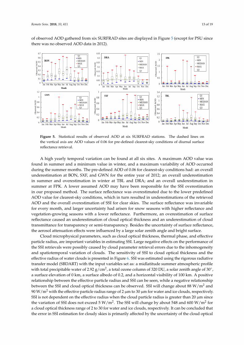
of observed AOD gathered from six SURFRAD sites are displayed in Figure 5 (except for PSU sincethere was no observed AOD data in 2012).Remote Sens. 2018, 10, x FOR PEER REVIEW 14 of 19

Figure 5. Statistical results of observed AOD at six SURFRAD stations. The dashed lines on the vertical axis are AOD values of 0.06 for pre-defined clearest-sky conditions of diurnal surface reflectance retrieval.

Cloud microphysical parameters, such as cloud optical thickness, thermal phase, and effective particle radius, are important variables in estimating SSI. Large negative effects on the performance of the SSI retrievals were possibly caused by cloud parameter retrieval errors due to the inhomogeneity and spatiotemporal variation of clouds. The sensitivity of SSI to cloud optical thickness and the effective radius of water clouds is presented in Figure 6. SSI was estimated using the rigorous radiative transfer model (SBDART) with the input variables set as: a midlatitude summer atmospheric profile with total precipitable water of 2.92 g/cm2, a total ozone column of 320 DU, a solar zenith angle of 30°, a surface elevation of 0 km, a surface albedo of 0.2, and a horizontal visibility of 100 km. A positive relationship between the effective particle radius and SSI can be seen, while a negative relationship between the SSI and cloud optical thickness can be observed. SSI will change about 88 W/m2 and 90 W/m2 with the effective particle radius range of 2 μm to 30 μm for water and ice clouds, respectively. SSI is not dependent on the effective radius when the cloud particle radius is greater than 20 μm since the variation of SSI does not exceed 5 W/m2. The SSI will change by about 548 and 600 W/m2 for a cloud optical thickness range of 2 to 30 for water and ice clouds, respectively. It can be concluded that the error in SSI estimation for cloudy skies is primarily affected by the uncertainty of the cloud optical thickness retrieval. There may be more than one solution for optical thickness and effective radius retrieval for optically thin clouds. The retrieved cloud optical thickness only represents 20–40% of the total optical thickness of the total cloud layer for clouds having COT ≥8, as indicated by Nakajima [37]. This situation can partially explain the positive bias of SSI estimation for cloudy skies.

0

0.1

0.2

0.3

0.4

0.5

0.6

0.7

Jan Feb Mar Apr May Jun Jul Aug Sep Oct Nov Dec

Obs

erve

d A

OD

Month

BON

Q1MINMEDIANMAXQ3

0

0.05

0.1

0.15

0.2

0.25

0.3

0.35

Jan Feb Mar Apr May Jun Jul Sep Oct Nov Dec

Obs

erve

d A

OD

Month

DRA Q1MINMEDIANMAXQ3

0

0.5

1

1.5

2

2.5

Jan Feb Mar Apr May Jun Jul Aug Sep Oct Nov Dec

Obs

erve

d A

OD

Month

FPK Q1MINMEDIANMAXQ3

0

0.2

0.4

0.6

0.8

1

1.2

Jan Feb Mar Apr May Jun Jul Aug Sep Oct Nov Dec

Obs

erve

d A

OD

Month

GWNQ1MINMEDIANMAXQ3

0

0.2

0.4

0.6

0.8

1

Jan Feb Mar Apr May Jun Jul Aug Sep Oct Nov Dec

Obs

erve

d A

OD

Month

SXF Q1MINMEDIANMAXQ3

00.20.40.60.8

11.21.4

Jan Feb Mar Apr May Jun Jul Aug Sep Oct Nov Dec

Ob

serv

ed A

OD

Month

TBL Q1MINMEDIANMAXQ3

Figure 5. Statistical results of observed AOD at six SURFRAD stations. The dashed lines onthe vertical axis are AOD values of 0.06 for pre-defined clearest-sky conditions of diurnal surfacereflectance retrieval.

A high yearly temporal variation can be found at all six sites. A maximum AOD value wasfound in summer and a minimum value in winter, and a maximum variability of AOD occurredduring the summer months. The pre-defined AOD of 0.06 for clearest-sky conditions had: an overallunderestimation at BON, SXF, and GWN for the entire year of 2012; an overall underestimationin summer and overestimation in winter at TBL and DRA; and an overall underestimation insummer at FPK. A lower assumed AOD may have been responsible for the SSI overestimationin our proposed method. The surface reflectance was overestimated due to the lower predefinedAOD value for clearest-sky conditions, which in turn resulted in underestimations of the retrievedAOD and the overall overestimation of SSI for clear skies. The surface reflectance was invariablefor every month, and larger uncertainty had arisen for snow seasons with higher reflectance andvegetation-growing seasons with a lower reflectance. Furthermore, an overestimation of surfacereflectance caused an underestimation of cloud optical thickness and an underestimation of cloudtransmittance for transparency or semi-transparency. Besides the uncertainty of surface reflectance,the aerosol attenuation effects were influenced by a large solar zenith angle and bright surface.

Cloud microphysical parameters, such as cloud optical thickness, thermal phase, and effectiveparticle radius, are important variables in estimating SSI. Large negative effects on the performance ofthe SSI retrievals were possibly caused by cloud parameter retrieval errors due to the inhomogeneityand spatiotemporal variation of clouds. The sensitivity of SSI to cloud optical thickness and theeffective radius of water clouds is presented in Figure 6. SSI was estimated using the rigorous radiativetransfer model (SBDART) with the input variables set as: a midlatitude summer atmospheric profilewith total precipitable water of 2.92 g/cm2, a total ozone column of 320 DU, a solar zenith angle of 30◦,a surface elevation of 0 km, a surface albedo of 0.2, and a horizontal visibility of 100 km. A positiverelationship between the effective particle radius and SSI can be seen, while a negative relationshipbetween the SSI and cloud optical thickness can be observed. SSI will change about 88 W/m2 and90 W/m2 with the effective particle radius range of 2 µm to 30 µm for water and ice clouds, respectively.SSI is not dependent on the effective radius when the cloud particle radius is greater than 20 µm sincethe variation of SSI does not exceed 5 W/m2. The SSI will change by about 548 and 600 W/m2 fora cloud optical thickness range of 2 to 30 for water and ice clouds, respectively. It can be concluded thatthe error in SSI estimation for cloudy skies is primarily affected by the uncertainty of the cloud optical

Remote Sens. 2018, 10, 411 14 of 19

thickness retrieval. There may be more than one solution for optical thickness and effective radiusretrieval for optically thin clouds. The retrieved cloud optical thickness only represents 20–40% of thetotal optical thickness of the total cloud layer for clouds having COT ≥8, as indicated by Nakajima [37].This situation can partially explain the positive bias of SSI estimation for cloudy skies.

Remote Sens. 2018, 10, x FOR PEER REVIEW 14 of 19

Figure 5. Statistical results of observed AOD at six SURFRAD stations. The dashed lines on the vertical axis are AOD values of 0.06 for pre-defined clearest-sky conditions of diurnal surface reflectance retrieval.

Cloud microphysical parameters, such as cloud optical thickness, thermal phase, and effective particle radius, are important variables in estimating SSI. Large negative effects on the performance of the SSI retrievals were possibly caused by cloud parameter retrieval errors due to the inhomogeneity and spatiotemporal variation of clouds. The sensitivity of SSI to cloud optical thickness and the effective radius of water clouds is presented in Figure 6. SSI was estimated using the rigorous radiative transfer model (SBDART) with the input variables set as: a midlatitude summer atmospheric profile with total precipitable water of 2.92 g/cm2, a total ozone column of 320 DU, a solar zenith angle of 30°, a surface elevation of 0 km, a surface albedo of 0.2, and a horizontal visibility of 100 km. A positive relationship between the effective particle radius and SSI can be seen, while a negative relationship between the SSI and cloud optical thickness can be observed. SSI will change about 88 W/m2 and 90 W/m2 with the effective particle radius range of 2 μm to 30 μm for water and ice clouds, respectively. SSI is not dependent on the effective radius when the cloud particle radius is greater than 20 μm since the variation of SSI does not exceed 5 W/m2. The SSI will change by about 548 and 600 W/m2 for a cloud optical thickness range of 2 to 30 for water and ice clouds, respectively. It can be concluded that the error in SSI estimation for cloudy skies is primarily affected by the uncertainty of the cloud optical thickness retrieval. There may be more than one solution for optical thickness and effective radius retrieval for optically thin clouds. The retrieved cloud optical thickness only represents 20–40% of the total optical thickness of the total cloud layer for clouds having COT ≥8, as indicated by Nakajima [37]. This situation can partially explain the positive bias of SSI estimation for cloudy skies.

0

0.1

0.2

0.3

0.4

0.5

0.6

0.7

Jan Feb Mar Apr May Jun Jul Aug Sep Oct Nov Dec

Obs

erve

d A

OD

Month

BON

Q1MINMEDIANMAXQ3

0

0.05

0.1

0.15

0.2

0.25

0.3

0.35

Jan Feb Mar Apr May Jun Jul Sep Oct Nov Dec

Obs

erve

d A

OD

Month

DRA Q1MINMEDIANMAXQ3

0

0.5

1

1.5

2

2.5

Jan Feb Mar Apr May Jun Jul Aug Sep Oct Nov Dec

Obs

erve

d A

OD

Month

FPK Q1MINMEDIANMAXQ3

0

0.2

0.4

0.6

0.8

1

1.2

Jan Feb Mar Apr May Jun Jul Aug Sep Oct Nov Dec

Obs

erve

d A

OD

Month

GWNQ1MINMEDIANMAXQ3

0

0.2

0.4

0.6

0.8

1

Jan Feb Mar Apr May Jun Jul Aug Sep Oct Nov Dec

Obs

erve

d A

OD

Month

SXF Q1MINMEDIANMAXQ3

00.20.40.60.8

11.21.4

Jan Feb Mar Apr May Jun Jul Aug Sep Oct Nov Dec

Ob

serv

ed A

OD

Month

TBL Q1MINMEDIANMAXQ3

Figure 6. The sensitivity of SSI to cloud optical thickness (given an effective particle radius of 20 µm)and effective particle radius (given a cloud optical thickness of 20) for water clouds (left) and iceclouds (right).

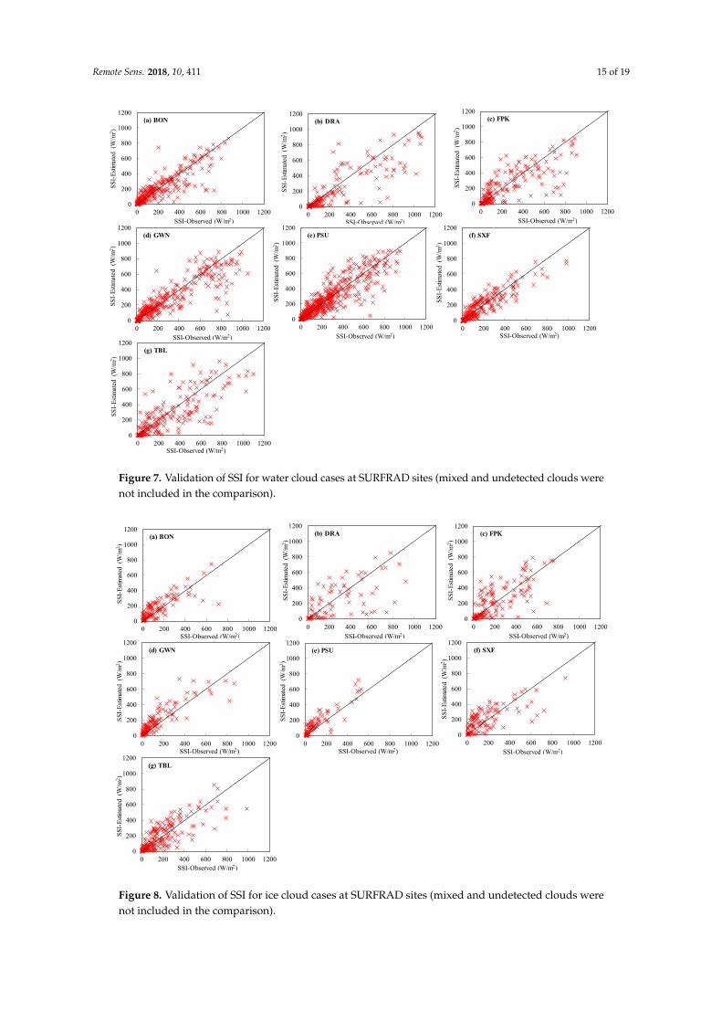
An overall underestimation of SSI with a maximum bias of 62.5 W/m2 and a minimum of 1 W/m2

for water clouds is indicated in Figure 7 and Table 6. All scatterplots for water and ice clouds areuniformly distributed between the line of 1:1. The RMSE has a maximum value of 177.6 W/m2 at DRA,thereby exceeding the values for clear skies (61.4 W/m2) by a factor of three. The minimum RMSE valueis 80.2 W/m2 at SXF, which is nearly the same as clear skies. Compared with water clouds, ice cloudstend to have a larger RMSE and a lower correlation coefficient (Figure 8, Table 6). The validationresults for ice cloud cases reveal a negative bias at DRA and TBL, which have an elevation greater than1000 m. The largest RMSE for ice clouds was 211.3 W/m2, which is about 75.3% of the systematic error.The relative accuracy of the modeled SSI for ice cloud cases is lower than 40%. This might be causedby the ice crystal density, particle size, shape, or direction, which are difficult to derive and describefor accurate scattering computation.

Besides the uncertainty of the input variables derived from satellite data, large uncertainty mayarise from the assumption of plane-parallel, homogeneous atmospheric conditions. Furthermore,a one-dimensional atmospheric transfer model cannot deal with the geometrical effects of scatteringfrom a higher solar zenith. The model is less reliable when the sub-pixel is partially cloudy, or whena rapid change in the atmospheric profile occurs during satellite observations.

Table 6. Validation results at seven SURFRAD stations for water and ice clouds.

SiteWater Clouds Ice Clouds Mixed

CloudsUndetected

Clouds

R2 BiasW/m2 (%)

RMSEW/m2 (%) NO. R2 Bias

W/m2 (%)RMSE

W/m2 (%) NO. NO. NO.

BON 0.74 −8 (−3.5) 106 (49.5) 280 0.66 27 (19.8) 93 (68.7) 121 222 31DRA 0.70 −63 (−21.0) 178 (59.6) 149 0.38 −44 (−15.7) 211 (75.3) 78 74 20FPK 0.62 −25 (−10.0) 157 (63.7) 187 0.54 15 (6.6%) 150 (67.2) 133 220 34

GWN 0.78 −31 (−10.6) 136 (46.3) 326 0.75 45 (32.0) 101 (71.2) 130 181 44PSU 0.81 −1 (−0.42) 105 (43.7) 576 0.81 44 (35.8) 83 (67.7) 83 217 20SXF 0.80 −5 (−2.6) 80 (43.0) 233 0.49 29 (16.5) 135 (78.1) 109 243 47TBL 0.64 −38 (−12.9) 169 (57.5) 197 0.61 −0.2 (−0.1) 118 (61.1) 186 173 20

Remote Sens. 2018, 10, 411 15 of 19

Remote Sens. 2018, 10, x FOR PEER REVIEW 15 of 19

clouds, ice clouds tend to have a larger RMSE and a lower correlation coefficient (Figure 8, Table 6). The validation results for ice cloud cases reveal a negative bias at DRA and TBL, which have an elevation greater than 1000 m. The largest RMSE for ice clouds was 211.3 W/m2, which is about 75.3% of the systematic error. The relative accuracy of the modeled SSI for ice cloud cases is lower than 40%. This might be caused by the ice crystal density, particle size, shape, or direction, which are difficult to derive and describe for accurate scattering computation.

Besides the uncertainty of the input variables derived from satellite data, large uncertainty may arise from the assumption of plane-parallel, homogeneous atmospheric conditions. Furthermore, a one-dimensional atmospheric transfer model cannot deal with the geometrical effects of scattering from a higher solar zenith. The model is less reliable when the sub-pixel is partially cloudy, or when a rapid change in the atmospheric profile occurs during satellite observations.

Table 6. Validation results at seven SURFRAD stations for water and ice clouds.

Site Water Clouds Ice Clouds

Mixed Clouds

UndetectedClouds

R2 Bias

W/m2 (%) RMSE

W/m2 (%) NO. R2

BiasW/m2 (%)

RMSEW/m2 (%)

NO. NO. NO.

BON 0.74 −8 (−3.5) 106 (49.5) 280 0.66 27 (19.8) 93 (68.7) 121 222 31 DRA 0.70 −63 (−21.0) 178 (59.6) 149 0.38 −44 (−15.7) 211 (75.3) 78 74 20 FPK 0.62 −25 (−10.0) 157 (63.7) 187 0.54 15 (6.6%) 150 (67.2) 133 220 34

GWN 0.78 −31 (−10.6) 136 (46.3) 326 0.75 45 (32.0) 101 (71.2) 130 181 44 PSU 0.81 −1 (−0.42) 105 (43.7) 576 0.81 44 (35.8) 83 (67.7) 83 217 20 SXF 0.80 −5 (−2.6) 80 (43.0) 233 0.49 29 (16.5) 135 (78.1) 109 243 47 TBL 0.64 −38 (−12.9) 169 (57.5) 197 0.61 −0.2 (−0.1) 118 (61.1) 186 173 20

Figure 7. Validation of SSI for water cloud cases at SURFRAD sites (mixed and undetected clouds were not included in the comparison).

0

200

400

600

800

1000

1200

0 200 400 600 800 1000 1200

SSI-

Estim

ated

(W

/m2 )

SSI-Observed (W/m2)

(a) BON

0

200

400

600

800

1000

1200

0 200 400 600 800 1000 1200

SSI-

Estim

ated

(W

/m2 )

SSI-Observed (W/m2)

(b) DRA

0

200

400

600

800

1000

1200

0 200 400 600 800 1000 1200

SSI-

Estim

ated

(W

/m2 )

SSI-Observed (W/m2)

(c) FPK

0

200

400

600

800

1000

1200

0 200 400 600 800 1000 1200

SSI-

Estim

ated

(W

/m2 )

SSI-Observed (W/m2)

(d) GWN

0

200

400

600

800

1000

1200

0 200 400 600 800 1000 1200

SSI-

Estim

ated

(W

/m2 )

SSI-Observed (W/m2)

(e) PSU

0

200

400

600

800

1000

1200

0 200 400 600 800 1000 1200

SSI-

Estim

ated

(W

/m2 )

SSI-Observed (W/m2)

(f) SXF

0

200

400

600

800

1000

1200

0 200 400 600 800 1000 1200

SSI-

Estim

ated

(W

/m2 )

SSI-Observed (W/m2)

(g) TBL

Figure 7. Validation of SSI for water cloud cases at SURFRAD sites (mixed and undetected clouds werenot included in the comparison).

Remote Sens. 2018, 10, x FOR PEER REVIEW 16 of 19

Figure 8. Validation of SSI for ice cloud cases at SURFRAD sites (mixed and undetected clouds were not included in the comparison).

5. Conclusions

The paper describes a novel approach to estimating surface solar irradiance (SSI) from a combined geostationary satellite image, MODIS land-surface albedo, and NCEP CFSR data. Aerosol optical thickness and cloud parameters (cloud phase, effective particle radius, and cloud optical thickness) were directly retrieved from the visible channel of geostationary satellite images for clear and cloudy skies. Total precipitable water was derived from the NCEP data, and other atmospheric variables, such as ozone, carbon dioxide, and trace gases, were not considered in our SSI estimation. The SSI was obtained by searching for and linearly interpolating a pre-calculated lookup table, which was created using the one-dimensional radiative transfer model for computational efficiency at the cost of calculation accuracy.

The validation was performed via station observations at SURFRAD and other developed algorithms were used with input from satellite data on an instantaneous basis to evaluate the performance of the estimates. The results demonstrated that our method could effectively retrieve instantaneous SSI with correlation coefficients of 0.94, 0.69, and 0.89, and an overall RMSE of 80.0 W/m2 (16.8%), 127.6 W/m2 (55.1%), and 99.5 W/m2 (25.5%) for clear-sky, cloudy-sky, and all-sky conditions, respectively. Our algorithm generally overestimated the SSI for clear- and all-sky conditions. Uncertainty analysis revealed that the accuracy of AOD retrieval was largely dependent upon diurnal surface reflectance. An overestimation of surface reflectance resulted in an underestimation of AOD and led to an overestimation of SSI. Large uncertainty may arise for optically thin clouds due to the ambiguous solutions for cloud optical thickness and effective radius. The RMSE for ice clouds is generally larger than water clouds since the radiative transfer process for ice clouds is mainly affected by ice crystal shape and particle size, which are difficult to directly retrieve with acceptable accuracy. In summary, our proposed method holds great promise for accurately estimating regional or global SSI and conducting research on Earth’s energy budget using products from geostationary satellites, such as FY2, Himawari-8, MTG, and MODIS.

0

200

400

600

800

1000

1200

0 200 400 600 800 1000 1200

SSI-

Estim

ated

(W

/m2 )

SSI-Observed (W/m2)

(a) BON

0

200

400

600

800

1000

1200

0 200 400 600 800 1000 1200

SSI-

Estim

ated

(W

/m2 )

SSI-Observed (W/m2)

(b) DRA

0

200

400

600

800

1000

1200

0 200 400 600 800 1000 1200

SSI-

Estim

ated

(W

/m2 )

SSI-Observed (W/m2)

(c) FPK

0

200

400

600

800

1000

1200

0 200 400 600 800 1000 1200

SSI-

Estim

ated

(W

/m2 )

SSI-Observed (W/m2)

(d) GWN

0

200

400

600

800

1000

1200

0 200 400 600 800 1000 1200

SSI-

Estim

ated

(W

/m2 )

SSI-Observed (W/m2)

(e) PSU

0

200

400

600

800

1000

1200

0 200 400 600 800 1000 1200

SSI-

Estim

ated

(W

/m2 )

SSI-Observed (W/m2)

(f) SXF

0

200

400

600

800

1000

1200

0 200 400 600 800 1000 1200

SSI-

Estim

ated

(W

/m2 )

SSI-Observed (W/m2)

(g) TBL

Figure 8. Validation of SSI for ice cloud cases at SURFRAD sites (mixed and undetected clouds werenot included in the comparison).

Remote Sens. 2018, 10, 411 16 of 19

5. Conclusions

The paper describes a novel approach to estimating surface solar irradiance (SSI) from a combinedgeostationary satellite image, MODIS land-surface albedo, and NCEP CFSR data. Aerosol opticalthickness and cloud parameters (cloud phase, effective particle radius, and cloud optical thickness)were directly retrieved from the visible channel of geostationary satellite images for clear and cloudyskies. Total precipitable water was derived from the NCEP data, and other atmospheric variables,such as ozone, carbon dioxide, and trace gases, were not considered in our SSI estimation. The SSIwas obtained by searching for and linearly interpolating a pre-calculated lookup table, which wascreated using the one-dimensional radiative transfer model for computational efficiency at the cost ofcalculation accuracy.

The validation was performed via station observations at SURFRAD and other developedalgorithms were used with input from satellite data on an instantaneous basis to evaluate theperformance of the estimates. The results demonstrated that our method could effectively retrieveinstantaneous SSI with correlation coefficients of 0.94, 0.69, and 0.89, and an overall RMSE of80.0 W/m2 (16.8%), 127.6 W/m2 (55.1%), and 99.5 W/m2 (25.5%) for clear-sky, cloudy-sky, and all-skyconditions, respectively. Our algorithm generally overestimated the SSI for clear- and all-sky conditions.Uncertainty analysis revealed that the accuracy of AOD retrieval was largely dependent upon diurnalsurface reflectance. An overestimation of surface reflectance resulted in an underestimation of AODand led to an overestimation of SSI. Large uncertainty may arise for optically thin clouds due to theambiguous solutions for cloud optical thickness and effective radius. The RMSE for ice clouds isgenerally larger than water clouds since the radiative transfer process for ice clouds is mainly affectedby ice crystal shape and particle size, which are difficult to directly retrieve with acceptable accuracy.In summary, our proposed method holds great promise for accurately estimating regional or globalSSI and conducting research on Earth’s energy budget using products from geostationary satellites,such as FY2, Himawari-8, MTG, and MODIS.

Acknowledgments: This study was financially supported by the Strategic Priority Research Program of ChineseAcademy of Sciences (Grant No. XDA15012002, XDA15007502) and the National Natural Science Foundation ofChina (Grant No. 41771394, 41471335, 41201352). NCEP data are available via https://rda.ucar.edu/datasets/ds094.1/#!description. The in situ SSI data collected at the SURFRAD station in the United States are available athttps://www.esrl.noaa.gov/gmd/grad/surfrad/. GOES satellite imaging radiometer data are freely downloadablefrom https://www.class.ncdc.noaa.gov/saa/products/welcome.

Author Contributions: Hailong Zhang and Qinhuo Liu designed the research. Xiaozhou Xin processed thesatellite and observation data. Chong Huang evaluated and analyzed the model’s performance. Shanshan Yu andLi Li designed the cloud detection method.

Conflicts of Interest: The authors declare no conflict of interest.

References

1. Wild, M. Global dimming and brightening: A review. J. Geophys. Res. Atmos. 2009, 114. [CrossRef]2. Houborg, R.; Soegaard, H.; Emmerich, W.; Moran, S. Inferences of all-sky solar irradiance using Terra and

Aqua MODIS satellite data. Int. J. Remote Sens. 2007, 28, 4509–4535. [CrossRef]3. Huang, J.; Yu, H.; Guan, X.; Wang, G.; Guo, R. Accelerated dryland expansion under climate change.

Nat. Clim. Chang. 2016, 6, 166–171. [CrossRef]4. Zhang, X.; Liang, S.; Zhou, G.; Wu, H.; Zhao, X. Generating Global LAnd Surface Satellite incident shortwave

radiation and photosynthetically active radiation products from multiple satellite data. Remote Sens. Environ.2014, 152, 318–332. [CrossRef]

5. Trenberth, K.E. An imperative for climate change planning: Tracking Earth’s global energy. Curr. Opin.Environ. Sustain. 2009, 1, 19–27. [CrossRef]

6. Alexandri, G.; Georgoulias, A.K.; Meleti, C.; Balis, D.; Kourtidis, K.A.; Sanchez-Lorenzo, A.; Trentmann, J.;Zanis, P. A high resolution satellite view of surface solar radiation over the climatically sensitive region ofEastern Mediterranean. Atmos. Res. 2017, 188, 107–121. [CrossRef]

Remote Sens. 2018, 10, 411 17 of 19

7. Yang, K.; Koike, T.; Ye, B. Improving estimation of hourly, daily, and monthly solar radiation by importingglobal data sets. Agric. For. Meteorol. 2006, 137, 43–55. [CrossRef]

8. Wang, L.; Kisi, O.; Zounemat-kermani, M.; Ariel, G.; Zhu, Z.; Gong, W. Solar radiation prediction usingdifferent techniques: Model evaluation and comparison. Renew. Sustain. Energy Rev. 2016, 61, 384–397.[CrossRef]

9. Shamim, M.A.; Remesan, R.; Bray, M.; Han, D. An improved technique for global solar radiation estimationusing numerical weather prediction. J. Atmos. Sol. Terr. Phys. 2015, 129, 13–22. [CrossRef]

10. Zou, L.; Wang, L.; Lin, A.; Zhu, H.; Peng, Y.; Zhao, Z. Estimation of global solar radiation using an arti fi cialneural network based on an interpolation technique in southeast China. J. Atmos. Sol. Terr. Phys. 2016, 146,110–122. [CrossRef]

11. Xie, Y.; Sengupta, M.; Dudhia, J. A Fast All-sky Radiation Model for Solar applications (FARMS): Algorithmand performance evaluation. Sol. Energy 2016, 135, 435–445. [CrossRef]

12. Zou, L.; Wang, L.; Xia, L.; Lin, A.; Hu, B.; Zhu, H. Prediction and comparison of solar radiation usingimproved empirical models and Adaptive Neuro-Fuzzy Inference Systems. Renew. Energy 2017, 106, 343–353.[CrossRef]

13. Yeom, J.; Seo, Y.; Kim, D.; Han, K. Solar Radiation Received by Slopes Using COMS Imagery, a PhysicallyBased Radiation Model, and GLOBE. J. Sens. 2016, 2016, 4834579. [CrossRef]

14. Tang, W.; Qin, J.; Yang, K.; Liu, S.; Lu, N.; Niu, X. Retrieving high-resolution surface solar radiation withcloud parameters derived by combining MODIS and MTSAT data. Atmos. Chem. Phys. 2016, 16, 2543–2557.[CrossRef]

15. Arbizu-Barrena, C.; Ruiz-Arias, J.A.; Rodríguez-Benítez, F.J.; Pozo-Vázquez, D.; Tovar-Pescador, J. Short-termsolar radiation forecasting by advecting and diffusing MSG cloud index. Sol. Energy 2017, 155, 1092–1103.[CrossRef]

16. Perez, R.; Seals, R.; Zelenka, A. Comparing satellite remote sensing and ground network measurements forthe production of site/time specific irradiance data. Sol. Energy 1997, 60, 89–96. [CrossRef]

17. Bishop, J.K.B.; Rossow, W.B. Spatial and Temporal Variability of Global Surface Solar Irradiance.J. Geophys. Res. 1991, 96, 16839–16858. [CrossRef]

18. Li, Z.; Leighton, H. Global climatologies of solar radiation budgets at the surface and in the atmosphere from5 years of ERBE data. J. Geophys. Res. Atmos. 1993, 98, 4919–4930. [CrossRef]

19. Kalnay, E.; Kanamitsu, M.; Kistler, R.; Collins, W.; Deaven, D.; Gandin, L.; Iredell, M.; Saha, S.; White, G.;Woollen, J.; et al. The NCEP/NCAR 40-Year Reanalysis Project. Bull. Am. Meteorol. Soc. 1996, 77, 437–471.[CrossRef]

20. Kato, S.; Loeb, N.G.; Rose, F.G.; Doelling, D.R.; Rutan, D.A.; Caldwell, T.E.; Yu, L.; Weller, R.A. SurfaceIrradiances Consistent with CERES-Derived Top-of-Atmosphere Shortwave and Longwave Irradiances.J. Clim. 2012, 26, 2719–2740. [CrossRef]

21. Müller, R.; Pfeifroth, U.; Träger-Chatterjee, C.; Trentmann, J.; Cremer, R. Digging the METEOSAT treasure-3decades of solar surface radiation. Remote Sens. 2015, 7, 8067–8101. [CrossRef]

22. Liang, S.; Zhao, X.; Liu, S.; Yuan, W.; Cheng, X.; Xiao, Z.; Zhang, X.; Liu, Q.; Cheng, J.; Tang, H.; et al.A long-term Global LAnd Surface Satellite (GLASS) data-set for environmental studies. Int. J. Digit. Earth2013, 6, 5–33. [CrossRef]

23. Zhang, X.; Liang, S.; Wild, M.; Jiang, B. Analysis of surface incident shortwave radiation from four satelliteproducts. Remote Sens. Environ. 2015, 165, 186–202. [CrossRef]

24. Seager, R.; Blumenthal, M.B. Modeling Tropical Pacific Sea Surface Temperature with Satellite-Derived SolarRadiative Forcing. J. Clim. 1994, 7, 1943–1957. [CrossRef]

25. Pinker, R.T.; Laszlo, I. Effects of Spatial Sampling of Satellite Data on Derived Surface Solar Irradiance.J. Atmos. Ocean. Technol. 1991, 8, 96–107. [CrossRef]

26. Mathiesen, P.; Kleissl, J. Evaluation of numerical weather prediction for intra-day solar forecasting in thecontinental United States. Sol. Energy 2011, 85, 967–977. [CrossRef]

27. Lara-Fanego, V.; Ruiz-Arias, J.A.; Pozo-Vázquez, D.; Santos-Alamillos, F.J.; Tovar-Pescador, J. Evaluation ofthe WRF model solar irradiance forecasts in Andalusia (southern Spain). Sol. Energy 2012, 86, 2200–2217.[CrossRef]

Remote Sens. 2018, 10, 411 18 of 19

28. Liang, S.; Zheng, T.; Liu, R.; Fang, H.; Tsay, S.-C.; Running, S. Estimation of incident photosyntheticallyactive radiation from Moderate Resolution Imaging Spectrometer data. J. Geophys. Res. 2006, 111, D15208.[CrossRef]

29. Qin, J.; Tang, W.; Yang, K.; Lu, N.; Niu, X.; Liang, S. An efficient physically based parameterization to derivesurface solar irradiance based on satellite atmospheric products. J. Geophys. Res. Atmos. 2015, 120, 4975–4988.[CrossRef]

30. Sun, Z.; Liu, A. Fast scheme for estimation of instantaneous direct solar irradiance at the earth’s surface.Sol. Energy 2013, 98, 125–137. [CrossRef]

31. Alexandri, G.; Georgoulias, A.K.; Zanis, P.; Katragkou, E.; Tsikerdekis, A.; Kourtidis, K.; Meleti, C.On the ability of RegCM4 regional climate model to simulate surface solar radiation patterns over Europe:An assessment using satellite-based observations. Atmos. Chem. Phys. 2015, 15, 13195–13216. [CrossRef]

32. Chen, M.; Zhuang, Q.; He, Y. An efficient method of estimating downward solar radiation based on theMODIS observations for the use of land surface modeling. Remote Sens. 2014, 6, 7136–7157. [CrossRef]

33. Barzin, R.; Shirvani, A.; Lotfi, H. Estimation of daily average downward shortwave radiation from MODISdata using principal components regression method: Fars province case study. Int. Agrophys. 2017, 31, 23–34.[CrossRef]

34. Cano, D.; Monget, J.; Albuisson, M.; Guillard, H.; Regas, N.; Wald, L. A method for the determination of theglobal solar radiation from meteorological satellite data. Sol. Energy 1986, 37, 31–39. [CrossRef]

35. Castelli, M.; Stöckli, R.; Zardi, D.; Tetzlaff, A.; Wagner, J.E.; Belluardo, G.; Zebisch, M.; Petitta, M.The HelioMont method for assessing solar irradiance over complex terrain: Validation and improvements.Remote Sens. Environ. 2014, 152, 603–613. [CrossRef]

36. Linares-Rodriguez, A.; Ruiz-Arias, J.A.; Pozo-Vazquez, D.; Tovar-Pescador, J. An artificial neural networkensemble model for estimating global solar radiation from Meteosat satellite images. Energy 2013, 61,636–645. [CrossRef]

37. Nakajima, T.; King, M.D.; Nakajima, T.; King, M.D. Determination of the Optical Thickness and EffectiveParticle Radius of Clouds from Reflected Solar Radiation Measurements. Part I: Theory. J. Atmos. Sci. 1990,47, 1878–1893. [CrossRef]

38. Platnick, S.; King, M.D.; Ackerman, S.A.; Menzel, W.P.; Baum, B.A.; Riédi, J.C.; Frey, R.A. The MODIS cloudproducts: Algorithms and examples from terra. IEEE Trans. Geosci. Remote Sens. 2003, 41, 459–472. [CrossRef]

39. Nakajima, T.Y.; Nakajma, T. Wide-Area Determination of Cloud Microphysical Properties from NOAAAVHRR Measurements for FIRE and ASTEX Regions. J. Atmos. Sci. 1995, 52, 4043–4059. [CrossRef]

40. Roebeling, R.A.; Feijt, A.J.; Stammes, P. Cloud property retrievals for climate monitoring: Implicationsof differences between Spinning Enhanced Visible and Infrared Imager (SEVIRI) on METEOSAT-8 andAdvanced Very High Resolution Radiometer (AVHRR) on NOAA-17. J. Geophys. Res. Atmos. 2006, 111, 1–51.[CrossRef]

41. Deneke, H.M.; Feijt, A.J.; Roebeling, R.A. Estimating surface solar irradiance from METEOSATSEVIRI-derived cloud properties. Remote Sens. Environ. 2008, 112, 3131–3141. [CrossRef]

42. Saha, S.; Moorthi, S.; Wu, X.; Wang, J.; Nadiga, S.; Tripp, P.; Behringer, D.; Hou, Y.T.; Chuang, H.Y.; Iredell, M.;et al. The NCEP climate forecast system version 2. J. Clim. 2014, 27, 2185–2208. [CrossRef]

43. Augustine, J.A.; DeLuisi, J.J.; Long, C.N. SURFRAD—A National Surface Radiation Budget Network forAtmospheric Research. Bull. Am. Meteorol. Soc. 2000, 81, 2341–2357. [CrossRef]

44. Ricchiazzi, P.; Yang, S.; Gautier, C.; Sowle, D. SBDART: A Research and Teaching Software Tool forPlane-Parallel Radiative Transfer in the Earth’s Atmosphere. Bull. Am. Meteorol. Soc. 1998, 79, 2101–2114.[CrossRef]

45. Popp, C.; Hauser, A.; Foppa, N.; Wunderle, S. Remote sensing of aerosol optical depth over central Europefrom MSG-SEVIRI data and accuracy assessment with ground-based AERONET measurements. J. Geophys.Res. Atmos. 2007, 112, 1–16. [CrossRef]

46. D’Entremont, R.P.; Gustafson, G.B. Analysis of Geostationary Satellite Imagery Using a Temporal-DifferencingTechnique. Earth Interact. 2003, 7, 1–25. [CrossRef]

47. Choi, Y.S.; Ho, C.H.; Ahn, M.H.; Kim, Y.M. An exploratory study of cloud remote sensing capabilities ofthe Communication, Ocean and Meteorological Satellite (COMS) imagery. Int. J. Remote Sens. 2007, 28,4715–4732. [CrossRef]

Remote Sens. 2018, 10, 411 19 of 19

48. Huang, G.; Li, X.; Huang, C.; Liu, S.; Ma, Y.; Chen, H. Representativeness errors of point-scale ground-basedsolar radiation measurements in the validation of remote sensing products. Remote Sens. Environ. 2016, 181,198–206. [CrossRef]

49. Ryu, Y.; Jiang, C.; Kobayashi, H.; Detto, M. MODIS-derived global land products of shortwave radiationand diffuse and total photosynthetically active radiation at 5 km resolution from 2000. Remote Sens. Environ.2018, 204, 812–825. [CrossRef]

© 2018 by the authors. Licensee MDPI, Basel, Switzerland. This article is an open accessarticle distributed under the terms and conditions of the Creative Commons Attribution(CC BY) license (http://creativecommons.org/licenses/by/4.0/).