A Low-Power Low-Memory Real-Time ASR System

Outline

• Overview of Automatic Speech Recognition (ASR) systems

• Sub-vector clustering and parameter quantization

• Custom arithmetic back-end

• Power simulation

ASR System Organization

• Front-end – Transform signal into a set of

feature vectors• Back-end

– Given the feature vectors, find the most likely word sequence

– Accounts for 90% of the computation

• Model parameters – Learned offline

• Dictionary– Customizable– Requires embedded HMMs

Goal: Given a speech signal find the most likely corresponding sequence of words

Speechwaveform

FeatureExtraction

Modelparameters

Dictionary

LikelihoodEvaluation

ViterbiDecoding

Featurevectors

ObservationProbabilities

Embedded HMM Decoding Mechanism

1 T

open

the

window

ASR on Portable Devices• Problem

– Energy consumption is a major problem for mobile speech recognition applications

– Memory usage is a main component of energy consumption

• Goal– Minimize power consumption and

memory requirement while maintaining high recognition rate

• Approach– Sub-vector clustering and parameter

quantization– Customized architecture

Outline

• Overview of speech recognition

• Sub-vector clustering and parameter quantization

• Custom arithmetic back-end

• Power simulation

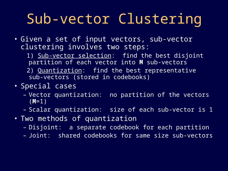
Sub-vector Clustering• Given a set of input vectors, sub-vector clustering

involves two steps: 1) Sub-vector selection: find the best disjoint partition of

each vector into M sub-vectors 2) Quantization: find the best representative sub-vectors

(stored in codebooks)

• Special cases– Vector quantization: no partition of the vectors (M=1)– Scalar quantization: size of each sub-vector is 1

• Two methods of quantization– Disjoint: a separate codebook for each partition– Joint: shared codebooks for same size sub-vectors

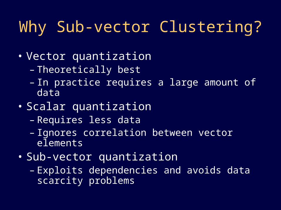
Why Sub-vector Clustering?

• Vector quantization– Theoretically best– In practice requires a large amount of data

• Scalar quantization– Requires less data– Ignores correlation between vector elements

• Sub-vector quantization– Exploits dependencies and avoids data

scarcity problems

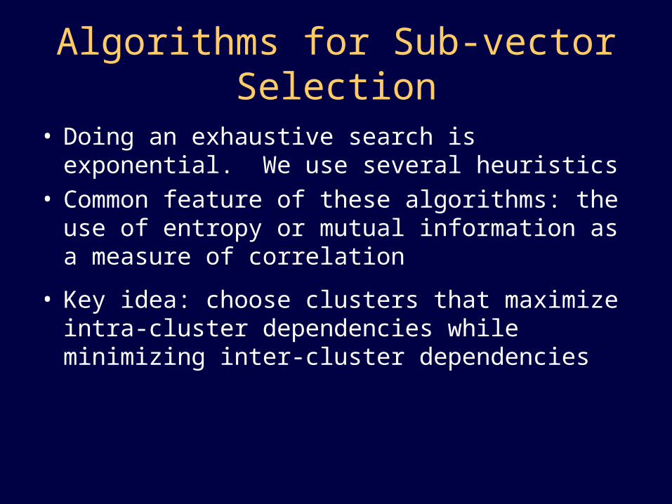
Algorithms for Sub-vector Selection

• Doing an exhaustive search is exponential. We use several heuristics

• Common feature of these algorithms: the use of entropy or mutual information as a measure of correlation

• Key idea: choose clusters that maximize intra-cluster dependencies while minimizing inter-cluster dependencies

Algorithms

• Pairwise MI-based greedy clustering– Rank vector component pairs by MI and

choose combination of pairs that maximizes overall MI.

• Linear entropy minimization– Choose clusters whose linear entropy,

normalized by the size of the cluster, is the lowest.

• Maximum clique quantization– Based on MI graph connectivity

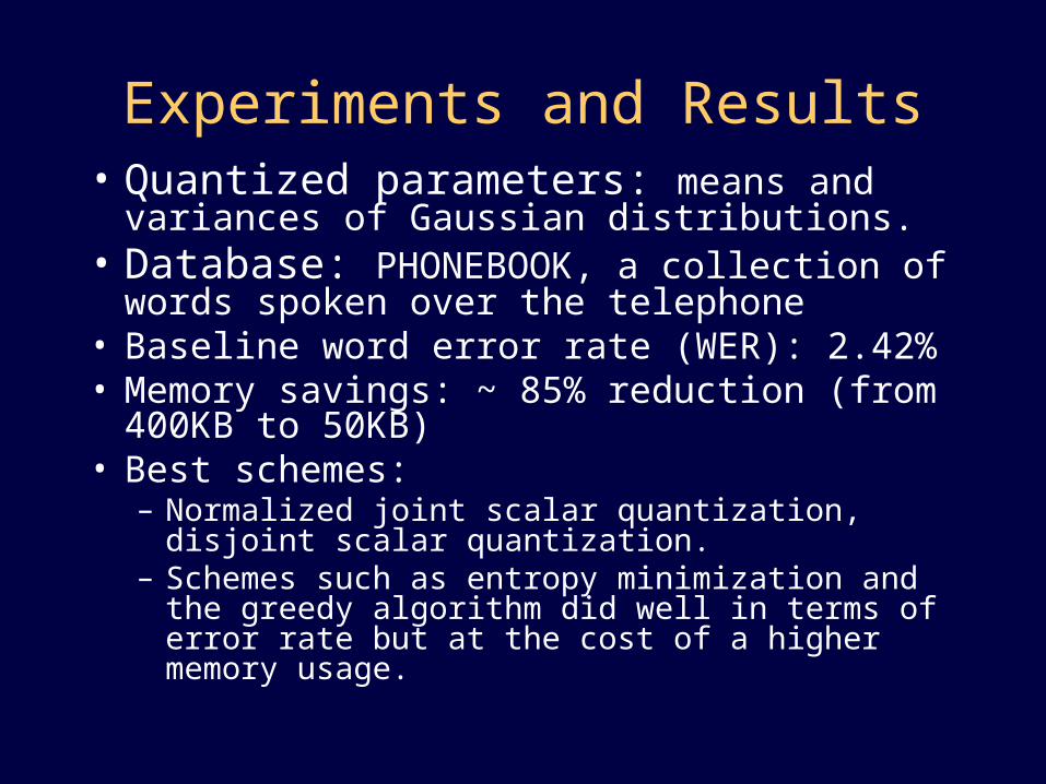
Experiments and Results• Quantized parameters: means and

variances of Gaussian distributions.• Database: PHONEBOOK, a collection of

words spoken over the telephone• Baseline word error rate (WER): 2.42%• Memory savings: ~ 85% reduction (from

400KB to 50KB)• Best schemes:

– Normalized joint scalar quantization, disjoint scalar quantization.

– Schemes such as entropy minimization and the greedy algorithm did well in terms of error rate but at the cost of a higher memory usage.

Quantization Algorithms Comparison: WER vs. Memory Usage

2

2.2

2.4

2.6

2.8

3

3.2

3.4

3.6

3.8

4

0 2 4 6 8 10 12 14 16 18 20

Total # of bits / total # of parameters

WE

R

disjoint scalar

disjoint greedy-1 pair

random-pair

entropy-min-2

max clique

joint scalar

vector quantization

Outline

• Overview of speech recognition

• Sub-vector clustering and parameter quantization

• Custom arithmetic back-end

• Power simulation

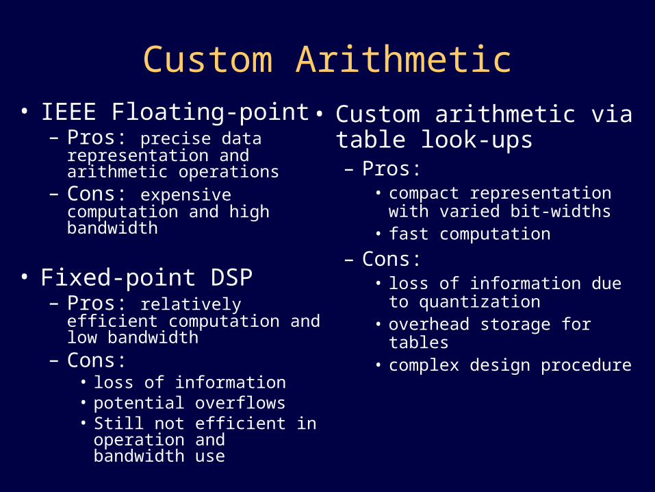
Custom Arithmetic• IEEE Floating-point

– Pros: precise data representation and arithmetic operations

– Cons: expensive computation and high bandwidth

• Fixed-point DSP– Pros: relatively efficient

computation and low bandwidth

– Cons:• loss of information• potential overflows• Still not efficient in

operation and bandwidth use

• Custom arithmetic via table look-ups– Pros:

• compact representation with varied bit-widths

• fast computation

– Cons:• loss of information due to

quantization• overhead storage for tables• complex design procedure

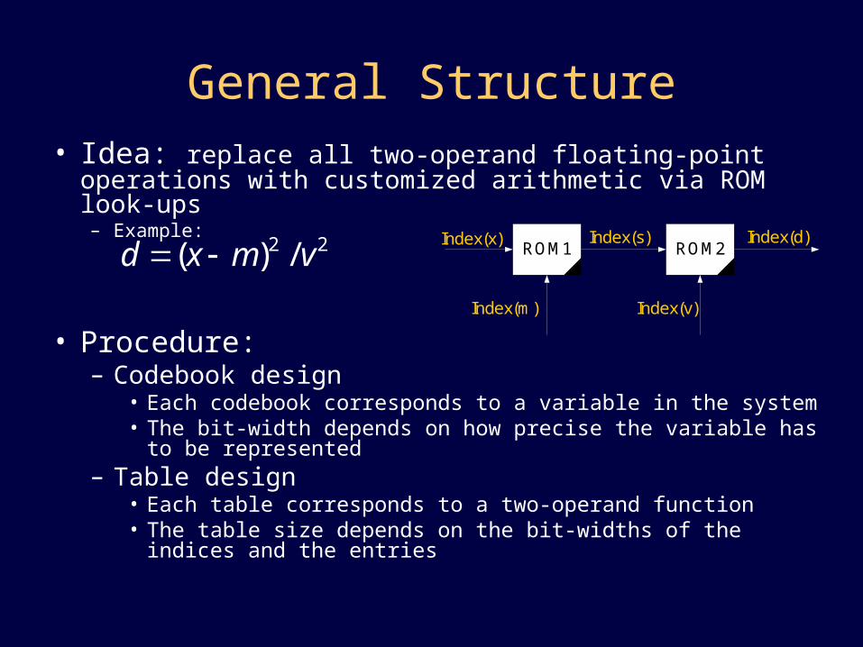
General Structure• Idea: replace all two-operand floating-point operations

with customized arithmetic via ROM look-ups– Example:

• Procedure:– Codebook design

• Each codebook corresponds to a variable in the system• The bit-width depends on how precise the variable has to be

represented– Table design

• Each table corresponds to a two-operand function• The table size depends on the bit-widths of the indices and the

entries

2 2( ) /d x m v ROM1Index(x)

Index(m)

Index(s)ROM2

Index(d)

Index(v)

Custom Arithmetic Design for the Likelihood Evaluation

• Issue: bounded accumulative variables

– Accumulating iteratively with a fixed number of iterations

– Large dynamic range, possibly too large for single codebook

• Solution: binary tree with one codebook per level

( ) ( ; , )j

j t i t i ii M

b O w N O

Y

X

Yt+1 = Yt + Xt+1

t = 0, 1, …,D

Custom Arithmetic Design for the Viterbi Search

• Issue: unbounded accumulative variables

– Arbitrarily long utterances; unbounded number of recursions

– Unpredictable dynamic range, bad for codebook design

• Solution: normalized forward probability– Dynamic programming still applies– No degradation in performance– A bounded dynamic range makes quantization

possible

1

( ) [ ( ( 1) )] ( ); 1, 2,...,N

j i ij j ti

t t a b O t T

( ) ( ) rtj jt t e

Optimization on Bit-Width Allocation

• Goal:– find the bit-width allocation scheme (bw1, bw2, bw3, …,

bwL) which minimizes the cost of resources while maintaining the baseline performance

• Approach: greedy algorithms– Optimal: intractable – Heuristics:

• Initialize (bw1, bw2, bw3, …, bwL) according to single-variable quantization results.

• Increase the bit-width of the variable which gives the best improvement concerning both performance and cost, until the performance is as good as the baseline

Three Greedy Algorithms

• Evaluation method: gradient

• Algorithms– Single-dimensional increment based on static

gradient– Single-dimensional increment based on dynamic

gradient– Pair-wise increment based on dynamic gradient

decrease in word error rate

increase in table storage

Results on Single-Variable Quantization

Parameters

1.5

2

2.5

3

3.5

4

4.5

1 2 3 4 5 6 7 8

mean variance responsibility transition prob.

Single-variable quantizationFree variables

1.5

2

2.5

3

3.5

4

4.5

1 2 3 4 5 6 7 8 9

bit-width

WE

R

s

d

a

c

q

p

alpha

Results• Likelihood evaluation:

– Replace floating-point processor with only 30KB for table storage, while the baseline recognition rate was maintained

– Reduce the offline storage for model parameters from 400KB to 90 KB

– Reduce the memory requirement for online recognition by 80%

Opitimal bit-width allocationfor likelihood evaluation

0

1

2

3

4

5

6

7

8

variable

bit

-wid

th

• Viterbi search: Currently we can quantize forward probability with 9 bits; Can we hit 8 bits?

Outline

• Overview of speech recognition

• Sub-vector clustering and parameter quantization

• Custom arithmetic back-end

• Power simulation

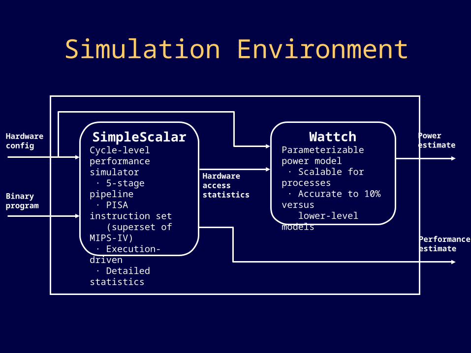
Simulation Environment

SimpleScalarCycle-level performance simulator · 5-stage pipeline · PISA instruction set (superset of MIPS-IV) · Execution-driven · Detailed statistics

WattchParameterizable power model · Scalable for processes · Accurate to 10% versus lower-level modelsBinary

program

Hardwareconfig

Hardware access statistics

Powerestimate

Performanceestimate

Our New Simulator

• ISA extended to support table look-ups• Three-operand instructions but need 4 values

for quantization– Two inputs– Output– Table to use

• Two options proposed:– One-step look-up -- different instruction for each table– Two-step look-up

• Set active table, used by any quantizations until reset• Perform look-up

Future Work

• Immediate future– Meet with architecture groups to discuss

relevant implementation details– Determine power parameters for look-up

tables

• Next steps– Generate power consumption data– Work with other groups for final

implementation