a machine learning approach to automatic chord … · a machine learning approach to automatic...
TRANSCRIPT
A Machine Learning Approach toAutomatic Chord Extraction
Matthew McVicar
Department of Engineering Mathematics
University of Bristol
A dissertation submitted to the University of Bristol in accordance with therequirements for award of the degree of Doctorate of Philosophy (PhD) in the
Faculty of Engineering
Word Count: 40,583

Abstract
In this thesis we introduce a machine learning based automatic chord recog-nition algorithm that achieves state of the art performance. This perfor-mance is realised by the introduction of a novel Dynamic Bayesian Net-work and chromagram feature vector, which concurrently recognises chords,keys and bass note sequences on a set of songs by The Beatles, Queen andZweieck.
In the months prior to the completion of this thesis, a large number ofnew, fully-labelled datasets have been released to the research community,meaning that the generalisation potential of models may be tested. Whensufficient training examples are available, we find that our model achievessimilar performance on both the well-known and novel datasets and statis-tically significantly outperforms a baseline Hidden Markov Model.
Our system is also able to learn from partially-labelled data. This is investi-gated through the use of guitar chord sequences obtained from the web. Intest, we align these sequences to the audio, accounting for changes in key,different interpretations, and missing structural information. We find thatthis approach increases recognition accuracy from on a set of songs by therock group The Beatles. Another use for these sequences is in a trainingscenario. Here we align over 1, 000 chord sequences to audio and use themas an additional training source. These data are exploited using curriculumlearning, where we see an improvement from when testing on a set of 715songs and evaluated on a complex chord alphabet.

Dedicated to my family

Acknowledgements
I would like to acknowledge the support, advice and guidance offered by
my supervisor, Tijl De Bie. I would also like to thank Yizhao Ni and Raul
Santos-Rodrıguez for their collaborations, proof-reading and friendship.
My work throughout this PhD was funded by the Bristol Centre for Com-
plexity Sciences (BCCS) and the Engineering and Physical Sciences Re-
search Council grant number EP/E501214/1. I am certain that the work
contained within this thesis would not have been possible without the in-
terdisciplinary teaching year at the BCCS, and am extremely grateful for
the staff, students and centre director John Hogan for the opportunity to
be taught by and work amongst these lecturers and students over the last
four years. Special thanks are also due to the BCCS co-ordinator, Sophie
Benoit.
Much of this thesis has built on previously existing concepts, many of which
have generously been made available for research purposes. In particular,
this work would not have been possible without the chord annotations by
Christopher Harte and Matthias Mauch (MIREX dataset), Nocolas Dooley
and Travis Kaufman (USpop dataset), and students at the Centre for In-
terdisciplinary Research in Music Media and Technology, McGill University
(Billboard dataset). I am also grateful to Dan Ellis for making his tuning
and beat-tracking scripts available online, and I made extensive use of the
software Sonic Visualiser by Chris Cannam at the Centre for Digital Mu-

sic at the Queen Mary, University of London; thank you for keeping this
fantastic software free.
Further thanks are due to Peter Flach, Nello Cristianini, Matthias Mauch,
Elena Hensinger, Owen Rackham, Antoni Matyjaszkiewicz, Angela Onslow,
Tom Irving, Harriet Mills, Petros Mina, Matt Oates, Jonathan Potts, Adam
Sardar, Donata Wasiuk, all the BCCS students past and present, and my
family: Liz, Brian and George McVicar.
Declaration
I declare that the work in this dissertation was carried out in accordance
with the requirements of the University’s Regulations and Code of Practice
for Research Degree Programmes and that it has not been submitted for
any other academic award. Except where indicated by specific reference in
the text, the work is the candidate’s own work. Work done in collaboration
with, or with the assistance of, others, is indicated as such. Any views ex-
pressed in the dissertation are those of the author.
SIGNED: ..................................................... DATE: .......................
Contents
List of Figures xi
List of Tables xvii
1 Introduction 1
1.1 Music as a Complex System . . . . . . . . . . . . . . . . . . . . . . . . . 1
1.2 Task Description and Motivation . . . . . . . . . . . . . . . . . . . . . . 3
1.2.1 Task Description . . . . . . . . . . . . . . . . . . . . . . . . . . . 3
1.2.2 Motivation . . . . . . . . . . . . . . . . . . . . . . . . . . . . . . 3
1.3 Objectives . . . . . . . . . . . . . . . . . . . . . . . . . . . . . . . . . . . 5
1.4 Contributions and thesis structure . . . . . . . . . . . . . . . . . . . . . 6
1.5 Relevant Publications . . . . . . . . . . . . . . . . . . . . . . . . . . . . 8
1.6 Conclusions . . . . . . . . . . . . . . . . . . . . . . . . . . . . . . . . . . 10
2 Background 13
2.1 Chords and their Musical Function . . . . . . . . . . . . . . . . . . . . . 13
2.1.1 Defining Chords . . . . . . . . . . . . . . . . . . . . . . . . . . . 13
2.1.2 Musical Keys and Chord Construction . . . . . . . . . . . . . . . 16
2.1.3 Chord Voicings . . . . . . . . . . . . . . . . . . . . . . . . . . . . 17
2.1.4 Chord Progressions . . . . . . . . . . . . . . . . . . . . . . . . . . 17
2.2 Literature Summary . . . . . . . . . . . . . . . . . . . . . . . . . . . . . 18
v
CONTENTS
2.3 Feature Extraction . . . . . . . . . . . . . . . . . . . . . . . . . . . . . . 24
2.3.1 Early Work . . . . . . . . . . . . . . . . . . . . . . . . . . . . . . 24
2.3.2 Constant-Q Spectra . . . . . . . . . . . . . . . . . . . . . . . . . 26
2.3.3 Background Spectra and Consideration of Harmonics . . . . . . . 26
2.3.4 Tuning Compensation . . . . . . . . . . . . . . . . . . . . . . . . 28
2.3.5 Smoothing/Beat Synchronisation . . . . . . . . . . . . . . . . . . 28
2.3.6 Tonal Centroid Vectors . . . . . . . . . . . . . . . . . . . . . . . 29
2.3.7 Integration of Bass Information . . . . . . . . . . . . . . . . . . . 30
2.3.8 Non-Negative Least Squares Chroma (NNLS) . . . . . . . . . . . 30
2.4 Modelling Strategies . . . . . . . . . . . . . . . . . . . . . . . . . . . . . 32
2.4.1 Template Matching . . . . . . . . . . . . . . . . . . . . . . . . . . 32
2.4.2 Hidden Markov Models . . . . . . . . . . . . . . . . . . . . . . . 34
2.4.3 Incorporating Key Information . . . . . . . . . . . . . . . . . . . 35
2.4.4 Dynamic Bayesian Networks . . . . . . . . . . . . . . . . . . . . 36
2.4.5 Language Models . . . . . . . . . . . . . . . . . . . . . . . . . . . 37
2.4.6 Discriminative Models . . . . . . . . . . . . . . . . . . . . . . . . 38
2.4.7 Genre-Specific Models . . . . . . . . . . . . . . . . . . . . . . . . 38
2.4.8 Emission Probabilities . . . . . . . . . . . . . . . . . . . . . . . . 39
2.5 Model Training and Datasets . . . . . . . . . . . . . . . . . . . . . . . . 39
2.5.1 Expert Knowledge . . . . . . . . . . . . . . . . . . . . . . . . . . 40
2.5.2 Learning from Fully-labelled Datasets . . . . . . . . . . . . . . . 41
2.5.3 Learning from Partially-labelled Datasets . . . . . . . . . . . . . 42
2.6 Evaluation Strategies . . . . . . . . . . . . . . . . . . . . . . . . . . . . . 42
2.6.1 Relative Correct Overlap . . . . . . . . . . . . . . . . . . . . . . 42
2.6.2 Chord Detail . . . . . . . . . . . . . . . . . . . . . . . . . . . . . 43
2.6.3 Cross-validation Schemes . . . . . . . . . . . . . . . . . . . . . . 44
2.6.4 The Music Information Retrieval Evaluation eXchange (MIREX) 45
vi

CONTENTS
2.7 The HMM for Chord Recognition . . . . . . . . . . . . . . . . . . . . . . 50
2.8 Conclusion . . . . . . . . . . . . . . . . . . . . . . . . . . . . . . . . . . 53
3 Chromagram Extraction 55
3.1 Motivation . . . . . . . . . . . . . . . . . . . . . . . . . . . . . . . . . . 55
3.1.1 The Definition of Loudness . . . . . . . . . . . . . . . . . . . . . 56
3.2 Preprocessing Steps . . . . . . . . . . . . . . . . . . . . . . . . . . . . . 58
3.3 Harmonic/Percussive Source Separation . . . . . . . . . . . . . . . . . . 58
3.4 Tuning Considerations . . . . . . . . . . . . . . . . . . . . . . . . . . . . 61
3.5 Constant Q Calculation . . . . . . . . . . . . . . . . . . . . . . . . . . . 61
3.6 Sound Pressure Level Calculation . . . . . . . . . . . . . . . . . . . . . . 63
3.7 A-Weighting & Octave Summation . . . . . . . . . . . . . . . . . . . . . 64
3.8 Beat Identification . . . . . . . . . . . . . . . . . . . . . . . . . . . . . . 65
3.9 Normalisation Scheme . . . . . . . . . . . . . . . . . . . . . . . . . . . . 65
3.10 Evaluation . . . . . . . . . . . . . . . . . . . . . . . . . . . . . . . . . . . 66
3.11 Conclusions . . . . . . . . . . . . . . . . . . . . . . . . . . . . . . . . . . 70
4 Dynamic Bayesian Network 73
4.1 Mathematical Framework . . . . . . . . . . . . . . . . . . . . . . . . . . 74
4.1.1 Mathematical Formulation . . . . . . . . . . . . . . . . . . . . . 74
4.1.2 Training the Model . . . . . . . . . . . . . . . . . . . . . . . . . . 76
4.1.3 Complexity Considerations . . . . . . . . . . . . . . . . . . . . . 77
4.2 Evaluation . . . . . . . . . . . . . . . . . . . . . . . . . . . . . . . . . . . 78
4.2.1 Experimental Setup . . . . . . . . . . . . . . . . . . . . . . . . . 79
4.2.2 Chord Accuracies . . . . . . . . . . . . . . . . . . . . . . . . . . . 80
4.2.3 Key Accuracies . . . . . . . . . . . . . . . . . . . . . . . . . . . . 81
4.2.4 Bass Accuracies . . . . . . . . . . . . . . . . . . . . . . . . . . . . 82
4.3 Complex Chords and Evaluation Strategies . . . . . . . . . . . . . . . . 83
vii

CONTENTS
4.3.1 Increasing the chord alphabet . . . . . . . . . . . . . . . . . . . . 83
4.3.2 Evaluation Schemes . . . . . . . . . . . . . . . . . . . . . . . . . 84
4.3.3 Experiments . . . . . . . . . . . . . . . . . . . . . . . . . . . . . 85
4.4 Conclusions . . . . . . . . . . . . . . . . . . . . . . . . . . . . . . . . . . 88
5 Exploiting Additional Data 89
5.1 Training across different datasets . . . . . . . . . . . . . . . . . . . . . . 90
5.1.1 Data descriptions . . . . . . . . . . . . . . . . . . . . . . . . . . . 91
5.1.2 Experiments . . . . . . . . . . . . . . . . . . . . . . . . . . . . . 93
5.2 Leave one out testing . . . . . . . . . . . . . . . . . . . . . . . . . . . . . 100
5.3 Learning Rates . . . . . . . . . . . . . . . . . . . . . . . . . . . . . . . . 102
5.3.1 Experiments . . . . . . . . . . . . . . . . . . . . . . . . . . . . . 102
5.3.2 Discussion . . . . . . . . . . . . . . . . . . . . . . . . . . . . . . . 105
5.4 Chord Databases for use in testing . . . . . . . . . . . . . . . . . . . . . 105
5.4.1 Untimed Chord Sequences . . . . . . . . . . . . . . . . . . . . . . 105
5.4.2 Constrained Viterbi . . . . . . . . . . . . . . . . . . . . . . . . . 108
5.4.3 Jump Alignment . . . . . . . . . . . . . . . . . . . . . . . . . . . 111
5.4.4 Experiments . . . . . . . . . . . . . . . . . . . . . . . . . . . . . 115
5.5 Chord Databases in Training . . . . . . . . . . . . . . . . . . . . . . . . 117
5.5.1 Curriculum Learning . . . . . . . . . . . . . . . . . . . . . . . . . 118
5.5.2 Alignment Quality Measure . . . . . . . . . . . . . . . . . . . . . 119
5.5.3 Results and Discussion . . . . . . . . . . . . . . . . . . . . . . . . 120
5.6 Conclusions . . . . . . . . . . . . . . . . . . . . . . . . . . . . . . . . . . 122
6 Conclusions 125
6.1 Summary . . . . . . . . . . . . . . . . . . . . . . . . . . . . . . . . . . . 125
6.2 Future Work . . . . . . . . . . . . . . . . . . . . . . . . . . . . . . . . . 130
viii

CONTENTS
References 135
A Songs used in Evaluation 151
B Relative chord durations 165
ix

CONTENTS
x

List of Figures
1.1 General approach to Automatic Chord Extraction. Features are ex-
tracted directly from audio that has been dissected into short time in-
stances known as frames, and then labelled with the aid of training data
or expert knowledge to yield a prediction file. . . . . . . . . . . . . . . . 3
1.2 Graphical representation of the main processes in this thesis. Rectangles
indicate data sources, whereas rounded rectangles represent processes.
Processes and data with asterisks form the bases of certain chapters.
Chromagram Extraction is the basis for chapter 3, the main decoding
process (HPA decoding) is covered in chapter 4, whilst training is the
basis of chapter 5. . . . . . . . . . . . . . . . . . . . . . . . . . . . . . . 11
2.1 Section of a typical chord annotation, showing onset time (first column),
offset time (second column), and chord label (third column). . . . . . . 18
2.2 A typical chromagram feature matrix, shown here for the opening to Let
It Be (Lennon/McCartney). Salience of pitch class p at time t is esti-
mated by the intensity of (p, t)th entry of the chromagram, with lighter
colours in this plot indicating higher energy (see colour bar between
chromagram and annotation). The reference (ground truth) chord an-
notation is also shown above for comparison, where we have reduced the
chords to major and minor classes for simplicity. . . . . . . . . . . . . . 25
xi

LIST OF FIGURES
2.3 Constant-Q spectrum of a piano playing a single A4 note. Note that, as
well as the fundamental at f0 =A4, there are harmonics at one octave
(A5) and one octave plus a just perfect fifth (E5). Higher harmonics
exist but are outside the frequency range considered here. Notice also
the slight presence of a fast-decaying subharmonic at two octaves down,
A2. . . . . . . . . . . . . . . . . . . . . . . . . . . . . . . . . . . . . . . . 27
2.4 Smoothing techniques for chromagram features. In 2.4a, we see a stan-
dard chromagram feature. Figure 2.4b shows a median filter over 20
frames, 2.4c shows a beat-synchronised chromagram. . . . . . . . . . . . 29
2.5 Treble (2.5a) and Bass (2.5b) Chromagrams, with the bass feature taken
over a frequency range of 55− 207 Hz in an attempt to capture inversions. 31
2.6 Regular (a) and NNLS (b) chromagram feature vectors. Note that the
NNLS chromagram is a beat-synchronised feature. . . . . . . . . . . . . 31
2.7 Template-based approach to the chord recognition task, showing chroma-
gram feature vectors, reference chord annotation and bit mask of chord
templates. . . . . . . . . . . . . . . . . . . . . . . . . . . . . . . . . . . . 33
2.8 Visualisation of a first order Hidden Markov Model (HMM) of length T.
Hidden states (chords) are shown as circular nodes, which emit observ-
able states (rectangular nodes, chroma frames). . . . . . . . . . . . . . 35
2.9 Two-chain HMM, here representing hidden nodes for Keys and Chords,
emitting Observed nodes. All possible hidden transitions are shown in
this figure, although these are rarely considered by researchers. . . . . . 36
2.10 Mathhias Mauch’s DBN. Hidden nodes Mi,Ki, Ci, Bi represent metric
position, key, chord and bass annotations, whilst observed nodes Cti and
Cbi represent treble and bass chromagrams. . . . . . . . . . . . . . . . . 37
xii
LIST OF FIGURES
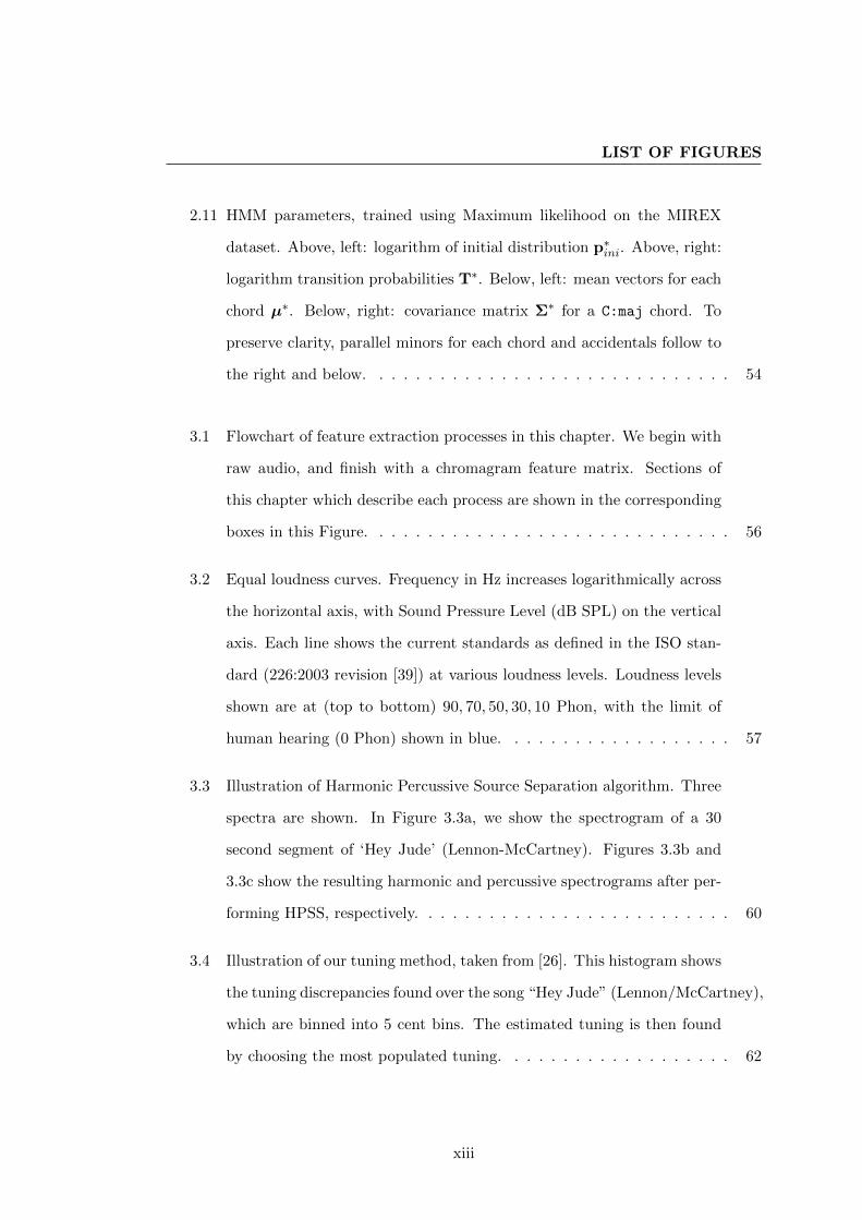
2.11 HMM parameters, trained using Maximum likelihood on the MIREX
dataset. Above, left: logarithm of initial distribution p∗ini. Above, right:
logarithm transition probabilities T∗. Below, left: mean vectors for each
chord µ∗. Below, right: covariance matrix Σ∗ for a C:maj chord. To
preserve clarity, parallel minors for each chord and accidentals follow to
the right and below. . . . . . . . . . . . . . . . . . . . . . . . . . . . . . 54
3.1 Flowchart of feature extraction processes in this chapter. We begin with
raw audio, and finish with a chromagram feature matrix. Sections of
this chapter which describe each process are shown in the corresponding
boxes in this Figure. . . . . . . . . . . . . . . . . . . . . . . . . . . . . . 56
3.2 Equal loudness curves. Frequency in Hz increases logarithmically across
the horizontal axis, with Sound Pressure Level (dB SPL) on the vertical
axis. Each line shows the current standards as defined in the ISO stan-
dard (226:2003 revision [39]) at various loudness levels. Loudness levels
shown are at (top to bottom) 90, 70, 50, 30, 10 Phon, with the limit of
human hearing (0 Phon) shown in blue. . . . . . . . . . . . . . . . . . . 57
3.3 Illustration of Harmonic Percussive Source Separation algorithm. Three
spectra are shown. In Figure 3.3a, we show the spectrogram of a 30
second segment of ‘Hey Jude’ (Lennon-McCartney). Figures 3.3b and
3.3c show the resulting harmonic and percussive spectrograms after per-
forming HPSS, respectively. . . . . . . . . . . . . . . . . . . . . . . . . . 60
3.4 Illustration of our tuning method, taken from [26]. This histogram shows
the tuning discrepancies found over the song “Hey Jude” (Lennon/McCartney),
which are binned into 5 cent bins. The estimated tuning is then found
by choosing the most populated tuning. . . . . . . . . . . . . . . . . . . 62
xiii
LIST OF FIGURES
3.5 Ground Truth extraction process. Given a ground truth annotation (top)
and set of beat locations (middle), we obtain the most prevalent chord
label between each beat to obtain beat-synchronous annotations. . . . . 66
3.6 Chromagram representations for the first 12 seconds of ‘Ticket to Ride’. 71
4.1 Model hierarchy for the Harmony Progression Analyser (HPA). Hidden
nodes (cicles) refer to chord (ci), key (ki) and bass note sequences (bi).
Chords and bass notes emit treble (Xti ) and bass (Cb
i ) chromagrams,
respectively. . . . . . . . . . . . . . . . . . . . . . . . . . . . . . . . . . . 74
4.2 Histograms of key accuracies of the Key-HMM (4.2a),Key-Bass-HMM
(4.2b) and HPA (4.2c) models. Accuracies shown are the averages over
100 repetitions of 3-fold cross-validation. . . . . . . . . . . . . . . . . . . 82
4.3 Testing Chord Precision and Note Precision from Table 4.4 for visual
comparison. . . . . . . . . . . . . . . . . . . . . . . . . . . . . . . . . . . 86
5.1 Section of a typical Billboard dataset entry before processing. . . . . . . 91
5.2 TRCO performances using an HMM trained and tested on all combi-
nation of datasets. Chord alphabet complexity increases in successive
graphs, with test groups increasing in clusters of bars. Training groups
follow the same ordering as the test data. . . . . . . . . . . . . . . . . . 97
5.3 Note Precision performances from Table 5.2 presented for visual com-
parison. Test sets follow the same order as the grouped training sets.
Abbreviations: Bill. = Billboard, C.K. = Carole King. . . . . . . . . . . 98
5.4 Comparative plots of HPA vs an HMM under various train/test scenarios
and chord alphabets. . . . . . . . . . . . . . . . . . . . . . . . . . . . . . 99
5.5 Distributions of data from Table 5.3. The number of songs attaining
each decile is shown over each of the four alphabets. . . . . . . . . . . . 101
xiv
LIST OF FIGURES
5.6 Learning rate of HPA when using increasing amounts of the Billboard
dataset. Training size increases along the x axis, with either Note or
Chord Precision measured on the y axis. Error bars of width 1 standard
deviation across the randomisations are also shown. . . . . . . . . . . . 104
5.7 Example e-chords chord and lyric annotation for “All You Need is Love”
(Lennon/McCartney), showing chord labels above lyrics. . . . . . . . . . 106
5.8 Example HMM topology for Figure 5.7. Shown here: (a) Alphabet
Constrained Viterbi (ACV), (b) Alphabet and Transition Constrained
Viterbi (ACV), (c) Untimed Chord Sequence Alignment (UCSA), (d)
Jump Alignment (JA). . . . . . . . . . . . . . . . . . . . . . . . . . . . 109
5.9 Example application of Jump Alignment for the song presented in Figure
5.7. By allowing jumps from ends of lines to previous and future lines,
we allow an alignment that follows the solid path, then jumps back to
the beginning of the song to repeat the verse chords before continuing
to the chorus. . . . . . . . . . . . . . . . . . . . . . . . . . . . . . . . . . 112
5.10 Results from Table 5.5, with UCSA omitted. Increasing amounts of
information from e-chords is used from left to right. Information used
is either simulated (ground truth, dotted line) or genuine (dashed and
solid lines). Performance is measured using Note Precision, and the
TRCO evaluation scheme is used throughout. . . . . . . . . . . . . . . . 117
xv
LIST OF FIGURES
5.11 Using aligned Untimed Chord Sequences as an additional training source.
The alignment quality threshold increases along the x–axis, with the
number of UCSs this corresponds to on the left y–axis. Baseline perfor-
mance is shown as a grey, dashed line; performance using the additional
UCSs is shown as the solid black line, with performance being measure
in TRCO on the right y–axis. Experiments using random training sets of
equal size to the black line with error bars of width 1 standard deviation
are shown as a black dot–and–dashed line. . . . . . . . . . . . . . . . . . 121
B.1 Histograms of relative chord durations across the entire dataset of fully-
labelled chord datasets used in this thesis (MIREX, USpop, Carole King,
Oasis, Billboard) . . . . . . . . . . . . . . . . . . . . . . . . . . . . . . . 165
xvi
List of Tables
2.1 Chronological summary of advances in automatic chord recognition from
audio, years 1999-2004. . . . . . . . . . . . . . . . . . . . . . . . . . . . . 19
2.2 Chronological Summary of advances in automatic chord recognition from
audio, years 2005-2006. . . . . . . . . . . . . . . . . . . . . . . . . . . . . 20
2.3 Chronological summary of advances in automatic chord recognition from
audio, years 2007-2008. . . . . . . . . . . . . . . . . . . . . . . . . . . . . 21
2.4 Chronological summary of advances in automatic chord recognition from
audio, 2009. . . . . . . . . . . . . . . . . . . . . . . . . . . . . . . . . . . 22
2.5 Chronological summary of advances in automatic chord recognition from
audio, years 2010-2011. . . . . . . . . . . . . . . . . . . . . . . . . . . . . 23
2.6 MIREX Systems from 2008-2009, sorted in each year by Total Rela-
tive Correct Overlap in the merged evaluation (confusing parallel ma-
jor/minor chords not considered an error). The best-performing pre-
trained/expert systems are underlined, best train/test systems are in
boldface. Systems where no data is available are shown by a dash (-). . 46
2.7 MIREX Systems from 2010-2011, sorted in each year by Total Relative
Correct Overlap. The best-performing pretrained/expert systems are
underlined, best train/test systems are in boldface. For 2011, systems
which obtained less than 0.35 TRCO are omitted. . . . . . . . . . . . . 47
xvii

LIST OF TABLES
3.1 Performance tests for different chromagram feature vectors, evaluated
using Average Relative Correct Overlap (ARCO) and Total Relative
Correct Overlap (TRCO). p−values for the Wilcoxon rank sum test on
successive features are also shown. . . . . . . . . . . . . . . . . . . . . . 68
4.1 Chord recognition performances using various crippled versions of HPA.
Performance is measured using Total Relative Correct Overlap (TRCO)
or Average Relative Correct Overlap (ARCO), and averaged over 100
repetitions of a 3-fold cross-validation experiment. Variances across these
repetitions are shown after each result, and the best results are shown
in bold. . . . . . . . . . . . . . . . . . . . . . . . . . . . . . . . . . . . . 80
4.2 Bass note recognition performances in models that recognise bass notes.
Performance is measured either using Total Relative Correct Overlap
(TRCO) or Average Relative Correct Overlap (ARCO), and is averaged
over 100 repetitions of a 3–fold cross–validation experiment. Variances
across these repetitions are shown after each result, and best results in
each column are in bold. . . . . . . . . . . . . . . . . . . . . . . . . . . . 82
4.3 Chord alphabets used for evaluation purposes. Abbreviations: MM =
Matthias Mauch, maj = major, min = minor, N = no chord, aug =
augmented, dim = diminished, sus2 = suspended 2nd, sus4 = suspended
4th, maj6 = major 6th, maj7 = major 7th, 7 = (dominant 7), min7 =
minor 7th, minmaj7 = minor, major 7th, hdim7 = half-diminished 7
(diminished triad, minor 7th). . . . . . . . . . . . . . . . . . . . . . . . . 83
4.4 HMM and HPA models under various evaluation schemes evaluated at
1, 000 Hz under TRCO. . . . . . . . . . . . . . . . . . . . . . . . . . . . 86
5.1 Performances across different training groups using an HMM. . . . . . . 94
xviii
LIST OF TABLES
5.2 Performances across all training/testing groups and all alphabets using
HPA, evaluated using Note and Chord Precision. . . . . . . . . . . . . . 98
5.3 Leave-one-out testing on all data with key annotations (Billboard, MIREX
and Carole King) across four chord alphabets. Chord Precision and Note
Precision are shown in the first row, with the variance across test songs
shown in the second. . . . . . . . . . . . . . . . . . . . . . . . . . . . . . 101
5.4 Pseudocode for the Jump Alignment algorithm. . . . . . . . . . . . . . . 114
5.5 Results using online chord annotations in testing. Amount of information
increases left to right, Note Precision is shown in the first 3 rows. p–
values using the Wilcoxon signed rank test for each result with respect
to that to the left of it are shown in rows 4–6. . . . . . . . . . . . . . . . 115
A.1 Oasis dataset, consisting of 5 chord annotations. . . . . . . . . . . . . . 151
A.2 Carole King dataset, consisting of 7 chord and key annotations. . . . . . 151
A.3 USpop dataset, consisting of 193 chord annotations. . . . . . . . . . . . 154
A.4 MIREX dataset, consisting of 217 chord and key annotations. . . . . . . 156
A.5 Billboard dataset, consisting of 522 chord and key annotations. . . . . . 163
xix

LIST OF TABLES
xx

List of Abbreviations
ACE Automatic Chord Extraction (task)
ACV Alphabet Constrained Viterbi
ARCO Average Relative Correct Overlap
ATCV Alphabet and Transition Constrained Viterbi
CD Compact Disc
CL Curriculum Learning
DBN Dynamic Bayesian Network
EDS Extractor Discovery System
FFT Fast Fourier Transform
xxi

LIST OF ABBREVIATIONS
GTUCS Ground Truth Untimed Chord Sequence
HMM Hidden Markov Model
HPA Harmony Progression Analyser
HPSS Harmonic Percussive Source Separation
JA Jump Alignment
MIDI Musical Instrument Digital Interface
MIR Music Information Retrieval
MIREX Music Information Retrieval Evaluation Exchange
ML Machine Learning
NNLS Non Negative Least Squares
PCP Pitch Class Profile
RCO Relative Correct Overlap
xxii
LIST OF ABBREVIATIONS
SALAMI Structural Analysis of Large Amounts of Music Information
SPL Sound Pressure Level
STFT Short Time Fourier Transform
SVM Support Vector Machine
TRCO Total Relative Correct Overlap
UCS Untimed Chord Sequence
UCSA Untimed Chord Sequence Alignment
WAV Windows Wave audio format
xxiii

LIST OF ABBREVIATIONS
xxiv
1
Introduction
This chapter serves as an introduction to the thesis as a whole. We will begin with a
brief discussion of how the project relates to the field of complexity sciences in section
1.1, before stating the task description and motivating our work in section 1.2. From
these motivations we will formulate our objectives in section 1.3. The main contribu-
tions of the work are then presented alongside the thesis structure in section 1.4. We
present a list of publications relevant to this thesis in section 1.5 before concluding in
section 1.6.
1.1 Music as a Complex System
Definitions of a complex system vary, but common traits that a complex system exhibit
are1:
1. It consist of many parts, out of whose interaction “emerges” behaviour not present
in the parts alone.
2. It is coupled to an environment with which it exchanges energy, information, or
other types of resources.
1from http://bccs.bristol.ac.uk/research/complexsystems.html
1
1. INTRODUCTION
3. It exhibits both order and randomness – in its (spatial) structure or (temporal)
behaviour.
4. The system has memory and feedback and can adapt itself accordingly.
Music as a complex system has been considered by many authors [22, 23, 66, 105]
but is perhaps best summarised by Johnson, in his book Two’s Company, Three’s Com-
plexity [41] when he states that music involves “a spontaneous interaction of collections
of objects (i.e., musicians)” and soloist patterns and motifs that are “interwoven with
original ideas in a truly complex way”.
Musical composition and performance is clearly an example of a complex system
as defined above. For example, melody, chord sequences and musical keys produce an
emergent harmonic structure which is not present in the isolated agents alone. Similarly,
live musicians often interact with their audiences, producing performances “...that arise
in an environment with audience feedback” [41], showing that energy and information
are shared between the system and its environment.
Addressing point 3, the most interesting and popular music falls somewhere between
order and randomness. For instance, signals which are entirely periodic (perfect sine
wave) or random (white noise) are uninteresting musically – signals which fall between
these two instances are where music is found. Finally, repetition is a key element of
music, with melodic, chordal and structural motifs appearing several times in a given
piece.
In most previous computational models of harmony, chords, keys and rhythm were
considered individual elements of music (with the exception of [62], see chapter 2), so
the original “complexity sciences” problem in this domain is a lack of understanding of
the interactions between these elements and a reductionist modelling methodology. To
counteract this, in this thesis we will investigate how an integrated model of chords,
keys, and basslines attempts to unravel the complexity of musical harmony. This will
2
1.2 Task Description and Motivation
be evidenced by the proposed model attaining recognition accuracies that exceed more
simplified approaches, which consider chords an isolated element of music instead of
part of a coherent complex system.
1.2 Task Description and Motivation
1.2.1 Task Description
Formally, Automatic Chord Extraction (ACE) is the task of assigning chord labels
and boundaries to a piece of musical audio, with minimal human involvement. The
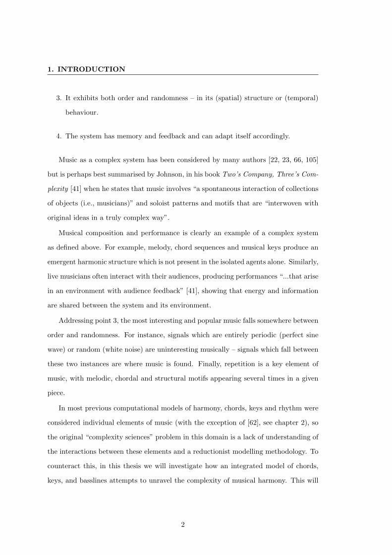
process of automatic chord extraction is shown in Figure 1.1. A digital audio waveform
is passed into a feature extractor, which then assigns labels to time chunks known
as “frames”. Labelling of frames is conducted by either the expert knowledge of the
algorithm designers, or is extracted from training data for previously labelled songs.
The final output is a file with start times, end times and chord labels.
0.000 0.175 N
0.175 1.852 C
1.852 3.454 G
3.454 4.720 A:min
4.720 5.126 A:min/b7
5.126 5.950 F:maj7
5.950 6.778 F:maj6
6.774 8.423 C
8.423 10.014 G
10.014 11.651 F
11.651 13.392 C
Feature
Extraction Decoding
Training Data/
Expert
Knowledge
Audio Frames
Figure 1.1: General approach to Automatic Chord Extraction. Features are extracteddirectly from audio that has been dissected into short time instances known as frames, andthen labelled with the aid of training data or expert knowledge to yield a prediction file.
1.2.2 Motivation
The motivation for our work is three-fold: we wish to develop a fully automatic chord
recognition system for amateur musicians that is capable of being used in higher-level
3
1. INTRODUCTION
tasks1 and is based entirely on machine learning techniques. We detail these goals
below.
Automatic Transcription for Amateur Musicians
Chords and chord sequences are mid-level features of music that are typically used
by hobby musicians and professionals as robust representations of a piece for playing
by oneself or in a group. However, annotating the (time-stamped) chords to a song
is a time-consuming task, even for professionals, and typically requires two or more
annotators to resolve disagreements, as well as an annotation time of 3–5 times the
length of the audio, per annotator [13].
In addition to this, many amateur musicians, despite being competent players, lack
sufficient musical training to annotate chord sequences accurately. This is evidenced
by the prevalence of “tab” (tablature, a form of visual representation of popular music)
websites, with hundreds of thousands of tabs and millions of users [60]. However,
such websites are of limited use for Music Information Retrieval (MIR) by themselves
because they lack onset times, which means they cannot be used in higher-level tasks
(see below). With this in mind, the advantage of developing an automatic system is
clear: such a technique could be scaled to work, unaided, across the thousands of songs
in a typical user’s digital music library and could be used by amateur musicians as an
educational or rehearsal tool.
Chords in Higher-level tasks
In addition to use by professional and amateur musicians, chords and chord sequences
have been used by the Music Information Retrieval (MIR) research community in the
simultaneous estimate of beats [89] and musical keys [16], as well as in higher-level tasks
1In this thesis, we describe low-level features as those extracted directly from the audio (duration,zero-crossing rate etc.), mid-level features as those which require significant processing beyond this,and high-level features as those which summarise an entire song. Tasks are defined as mid-level (forinstance) if they attempt to identify mid-level features.
4
1.3 Objectives
such as cover song identification [27], genre detection [91] and lyrics-to-audio alignment
[70]. Thus, advancement in automatic chord recognition will impact beyond the task
itself and lead to developments in some of the areas listed above.
A Machine Learning Approach
One may train a chord recognition system either by using expert knowledge or by mak-
ing use of previously available training examples, known as “ground truth”, through
Machine Learning (ML). In the annual MIREX (Music Information Retrieval Eval-
uation eXchange) evaluations, both approaches to the task are very competitive at
present, with algorithms in both cases exceeding 80% accuracy (see Subsection 2.6.4).
In any recognition task where the total number of examples is sufficiently small, an
expert system will be able to perform well, as there will likely be less variance in the
data, and one may specify parameters which fit the data well. At the other extreme, in
cases of large and varied test data, it is impossible to specify the parameters necessary
to attain good performance - a problem known as the acquisition bottleneck [31].
However, if sufficient training data are available for a task, machine learning systems
may lead to higher generalisation potential than expert systems. This point is specifi-
cally important in the domain of chord estimation, since a large number of new ground
truths have been made available in recent months, which means that the generalisation
of a machine-learning system may be tested. The prospect of good generalisation of an
ML system to unseen data is the third motivating factor for this work.
1.3 Objectives
The objectives of this thesis echo the motivations discussed above. However, we must
first investigate the literature to define the state of the art and see which techniques
have been used by previous researchers in the field. Thus a thorough review of the
5
1. INTRODUCTION
literature is the first main objective of this thesis.
Once this has been conducted, we may address the second objective: developing a
system that performs at the state of the art (discussions of evaluation strategies are
postponed until Section 2.6). This will involve the construction of two main facets: the
development of a new chromagram feature vector for representing harmony, and the
decoding of these features into chord sequences via a new graphical model.
Finally, we will investigate and exploit one of the main advantages of deploying a
machine learning based chord recognition: it may be retrained on new data as it arises.
Thus, our final objective will be to evaluate how our proposed system performs when
trained on recently available training data and also test the generalisation of our model
to new datasets.
1.4 Contributions and thesis structure
The four main contributions of this thesis are:
• A thorough review of the literature of automatic chord estimation, including the
MIREX evaluations and major publications in the area.
• The development of a new chromagram feature representation which is based on
the human perception of loudness of sounds.
• A new Dynamic Bayesian Network (DBN) which concurrently recognises the
chords, keys and basslines of popular music which, in addition to the above,
attains state of the art performance on a known set of ground truths.
• Detailed train/test scenarios using all the current data available for researchers
in the field, with additional use of online chord databases for use in the training
and testing phase.
6

1.4 Contributions and thesis structure
These contributions are highlighted in the main chapters of this thesis. A graphical
representation of our main algorithm, highlighting the thesis structure, is shown in
Figure 1.2. We also provide brief summaries of the remaining chapters:
Chapter 2: Background
In this chapter, the relevant background information to the field is given. We begin
with some preliminary definitions and discussions of the function of chords in Western
Popular music. We then give a detailed account of the literature to date, with partic-
ular focus on feature extraction, modelling strategies, training schemes and evaluation
techniques.
Chapter 3: Chromagram Extraction
Feature extraction is the focus of this chapter. We outline the motivation for loudness-
based chromagrams, and then describe each stage of their calculation. We follow this
by conducting experiments to highlight the efficacy of these features on a trusted set
of 217 popular recordings for which the ground truth sequences are known.
Chapter 4: Dynamic Bayesian Network
This chapter is concerned with our decoding process: a Dynamic Bayesian Network
with hidden nodes that represents chords, keys and basslines/inversions, which we call
the Harmony Progression Analyser (HPA). We begin by formalising the mathematics of
the model and decoding process, before incrementally increasing the model complexity
from a simple Hidden Markov Model (HMM) to HPA, by adding hidden nodes and
transitions.
These models are evaluated in accordance with the MIREX evaluations and are
shown to attain state of the art performance on a set of 25 chord states representing
the 12 major chords, 12 minor chords, and a No Chord symbol for periods of silence,
7
1. INTRODUCTION
speaking or for other times when no chord can be assigned. We finish this chapter
by introducing a wider set of chord alphabets and discuss how one might deal with
evaluating ACE systems on such alphabets.
Chapter 5: Exploiting Additional Data
In previous chapters, we used a trusted set of ground truth chord annotations which
have been used numerous times in the annual MIREX evaluations. However, recently
a number of new annotations have been made public, offering a chance to retrain HPA
on a set of new labels. To this end, chapter 5 deals with training and testing on
these datasets to ascertain whether learning can be transferred between datasets, and
also investigates learning rates for HPA. We then move on to discuss how partially
labelled data may be used in either testing or training a machine learning based chord
estimation algorithm, where we introduce a new method for aligning chord sequences
to audio called jump alignment and additionally an evaluation scheme for estimating
the alignment quality.
Chapter 6: Conclusion
This final chapter summarises the main findings of the thesis and suggests areas where
future research might be advisable.
1.5 Relevant Publications
A selection of relevant publications is presented in this section. Although the author
has had publications outside the domain of automatic chord estimation, the papers
presented here are entirely in this domain and relevant to this thesis. These works
also tie in the main contributions of the thesis: journal paper 3 is an extension of the
literature review from chapter 2, journal paper 1 [81] forms the basis of chapters 3 and
8

1.5 Relevant Publications
4, whilst journal paper 2 [74] and conference paper 1 [73] form the basis of chapter 5.
Journal Papers
• Y. Ni, M. McVicar, R. Santos-Rodriguez. and T. De Bie. An end-to-end machine
learning system for harmonic analysis of music. IEEE Transactions on Audio,
Speech and Language Processing [81]
[81] is based on early work (not otherwise published) by the author on using key-
information in chord recognition, which has guided the design of the structure the DBN
put forward in this paper. The structure of the DBN is also inspired by musicological
insights contributed by the thesis author. Early research by the author (not otherwise
published) on the use of the constant-Q transform for designing chroma features has
contributed to the design of the LBC feature introduced in this paper. All aspects of
the research were discussed in regular meetings involving all authors. The paper was
written predominantly by the first author, but all authors contributed original material.
• M. McVicar, Y. Ni, R. Santos-Rodriguez. and T. De Bie. Using Online Chord
Databases to Enhance Chord Recognition. Journal of New Music Research, Special
Issue on Music and Machine Learning [74]
The research into using alignment of untimed chord sequences for chord recognition was
initiated by Tijl De Bie and the thesis author. It first led to a workshop paper [72], and
[74] is an extension of this paper which includes also the Jump Alignment algorithm
which was developed by Yizhao Ni but discussed by all authors. The paper was written
collaboratively by all authors. The second author of [73] contributed insight and exper-
iments which did not make it into the final version of the paper, with remainder being
composed and conducted by the first author. The paper was predominantly written by
the first author.
9
1. INTRODUCTION
• M. McVicar, Y. Ni, R. Santos-Rodriguez. and T. De Bie. Automatic Chord
Estimation from Audio: A Review of the State of the Art (submitted). IEEE
Transactions on Audio, Speech and Language Processing [75]
Finally, journal paper three was researched and written primarily by the first author,
with contributions from the third author concerning ACE software.
Conference Papers
1. M. McVicar, Y. Ni, R. Santos-Rodriguez and T. De Bie. Leveraging noisy online
databases for use in chord recognition. In Proceedings of the 12th International
Society for Music Information Retrieval (ISMIR), 2011 [73]
1.6 Conclusions
In this chapter, we discussed the motivation for our subject: automatic chord esti-
mation. We also defined our main research objective: the development of a chord
recognition system based entirely on machine-learning techniques, which may take full
advantage of the newly released data sources that have become available. We went on
to list the main contributions to the field contained within this thesis, and how these
appear within the structure of the work. These contributions were also highlighted in
the main publications by the author.
10

1.6 Conclusions
Performance Evaluation scheme
Predic-on
Training audio
Fully labelled
training data
Partially labelled
training data
MLE parameters
Training Chromagram
Testing Chromagram
Test Audio
Partially labelled test
data
Chromagram Extraction (Chap 3)
Chromagram Extraction*
HPA training
(Chap. 5)
HPA decoder (Chap 4)
Fully labelled test data
Figure 1.2: Graphical representation of the main processes in this thesis. Rectanglesindicate data sources, whereas rounded rectangles represent processes. Processes and datawith asterisks form the bases of certain chapters. Chromagram Extraction is the basisfor chapter 3, the main decoding process (HPA decoding) is covered in chapter 4, whilsttraining is the basis of chapter 5.
11

1. INTRODUCTION
12
2
Background
This chapter is an introduction to the domain of automatic chord estimation. We begin
by describing chords and their function in musical theory in section 2.1. A chronological
account of the literature is given in section 2.2, which is discussed in detail in sections
2.3 - 2.6. We focus here on Feature extraction, Modelling strategies, Datasets and
Training, and finally Evaluation Techniques. Since their use is so ubiquitous in the field,
we devote section 2.7 to the Hidden Markov Model for automatic chord extraction. We
conclude the chapter in section 2.8.
2.1 Chords and their Musical Function
This section serves to introduce the theory behind our chosen subject: musical chords.
The definition and function of chords in musical theory is discussed, with particular
focus on Western Popular music, the genre on which our work will be conducted.
2.1.1 Defining Chords
Before discussing how chords are defined, we must first begin with the more fundamental
definitions of frequency and pitch. Musical instruments (including the voice) are able
13
2. BACKGROUND
to vibrate at a fixed number of oscillations per second, known as their fundamental
frequency, f0 measured in Hertz (Hz). Although frequencies higher (harmonics) and
lower (subharmonics) than f0 are produced simultaneously, we postpone the discussion
of this until section 2.3.
The word pitch, although colloquially similar to frequency, means something quite
different. Pitch is defined as the perceptual ordering of sounds on a frequency scale
[47]. Thus, pitch relates to how we are able to differentiate between lower and higher
fundamental frequencies. Pitch is approximately proportional to the logarithm of fre-
quency, and in Western equal-temperament, the fundamental frequency f of a pitch is
defined as
f = fref2n/12, n = {. . . ,−1, 0, 1, . . .}, (2.1)
where fref is a reference frequency, usually taken to be 440 Hz. The distance (interval)
between two adjacent pitches is known as a semitone, a tone being twice this distance.
Notice from Equation 2.1 that pitches 12 semitones apart have a frequency ratio of 2,
an interval known as an octave, which is a property captured in the notions of pitch
class and pitch height [112].
It has been noted that the human auditory system is able to distinguish pitch
classes, which refers to the value of n mod 12 in Equation 2.1, from pitch height,
which describes the value of b n12c, (b·c represents the floor function) [101]. This means
that, for example, we hear two frequencies an octave apart as the same note. This
phenomenon is known as octave equivalence and has been exploited by researchers in
the design of chromagram features (see section 2.3).
Pitches are often described using modern musical notation to avoid the use of irra-
tional frequency numbers. This is a combination of letters (pitch class) and numbers
(pitch height), where we define A4 = 440 Hz and higher pitches as coming from the
14
2.1 Chords and their Musical Function
pitch class set
PC = {C,C],D,D],E, F, F ],G,G]A,A],B} (2.2)
until we reach B4, when we loop round to C5 (analogously for lower pitches). In
this discussion and throughout this thesis we will assume equivalence between sharps
and flats, i.e. G]4 = A[4. We now turn our attention to collections of pitches played
together, which is intuitively the notion of a chord.
The word chord has many potential characterisations and there is no universally
agreed upon definition. For example, Merriam-Webster’s dictionary of English usage
[76] claims:
Definition 1. Everyone agrees that chord is used for a group of musical tones,
whilst Krolyi [42] is more specific, stating:
Definition 2. Two or more notes sounding simultaneously are known as a chord.
Note here the concept of pitches being played simultaneously. Note also that it is
not specified that the notes come from one particular voice, so that a chord may be
played by a collection of instruments. Such music is known as Polyphonic (conversely
Monophonic). The Harvard Dictionary of music [93] defines a chord more strictly as a
collection of three or more notes:
Definition 3. Three or more pitches sounded simultaneously or functioning as if
sounded simultaneously.
Here the definition stretches to allow notes played in succession to be a chord - a concept
known as an arpeggio. In this thesis, we define a chord to be a collection of 3 or more
notes played simultaneously. Note however that there will be times when we will need
to be more flexible when dealing with, for instance, pre-made ground truth datasets
such as those by Harte et al. [36]. In cases when datasets such as these contradict our
definition we will map them to a suitable chord to our best knowledge. For instance,
15
2. BACKGROUND
the aforementioned dataset contains examples such as A:(1,3), meaning an A and C]
note played simultaneously, which we will map to a C:maj chord. We now turn our
attention to how chords function within the theory of musical harmony.
2.1.2 Musical Keys and Chord Construction
In popular music, chords are not chosen randomly as collections of pitch classes. In-
stead, a key is used to define a suitable library of pitch classes and chords. The most
canonical example of a collection of pitch classes is the major scale, which, given a root
(starting note) is defined as the set of intervals Tone-Tone-Semitone-Tone-Tone-Tone-
Semitone. For instance, the key of C Major contains the pitch classes
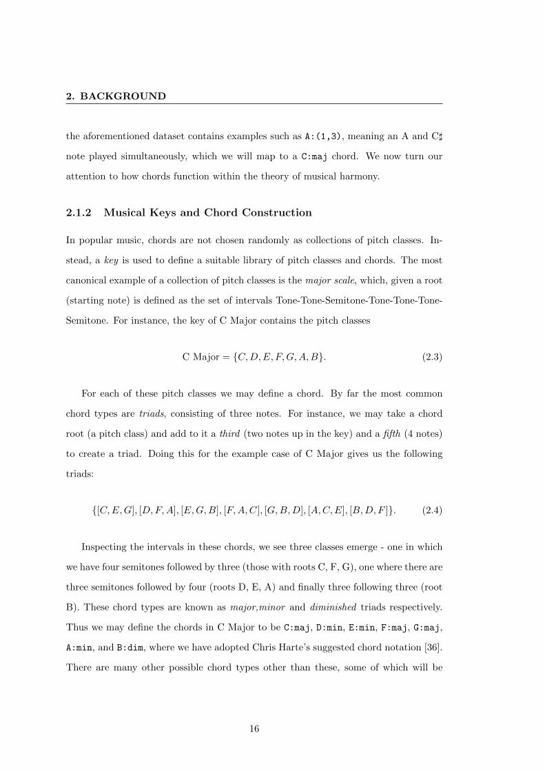
C Major = {C,D,E, F,G,A,B}. (2.3)
For each of these pitch classes we may define a chord. By far the most common
chord types are triads, consisting of three notes. For instance, we may take a chord
root (a pitch class) and add to it a third (two notes up in the key) and a fifth (4 notes)
to create a triad. Doing this for the example case of C Major gives us the following
triads:
{[C,E,G], [D,F,A], [E,G,B], [F,A,C], [G,B,D], [A,C,E], [B,D,F ]}. (2.4)
Inspecting the intervals in these chords, we see three classes emerge - one in which
we have four semitones followed by three (those with roots C, F, G), one where there are
three semitones followed by four (roots D, E, A) and finally three following three (root
B). These chord types are known as major,minor and diminished triads respectively.
Thus we may define the chords in C Major to be C:maj, D:min, E:min, F:maj, G:maj,
A:min, and B:dim, where we have adopted Chris Harte’s suggested chord notation [36].
There are many other possible chord types other than these, some of which will be
16

2.1 Chords and their Musical Function
considered in our model (see section 4.3).
We have presented the work here as chords being constructed from a key, although
one may conversely consider a collection of chords as defining a key. This thorny issue
was considered by Raphael [95] and a potential solution in modelling terms offered by
some authors [16, 57] by estimating the chords and keys simultaneously (see subsection
2.4 for more details on this strategy). Keys may also change throughout a piece, and
thus the associated chords in a piece may change (a process known as modulation).
This has been modelled by some authors, leading to an improvement in recognition
accuracy of chords [65].
2.1.3 Chord Voicings
On any instrument with a tonal range of over one octave, one has a choice as to which
order to play the notes in a given chord. For instance, C:maj = {C, E, G} can be
played as (C, E, G), (E, G, C) or (G, C, E). These are known as the root position, first
inversion and second inversion of a C Major chord respectively.
When constructing 12–dimensional chromagram vectors (see section 2.3), this poses
a problem: how are we to distinguish between inversions in recognition, or evaluation?
These issues will be dealt with in sections 2.4 and 2.6.
2.1.4 Chord Progressions
Chords are rarely considered in isolation and as such music composers generally collate
chords into a time series. A collection of chords played in sequence is known as a
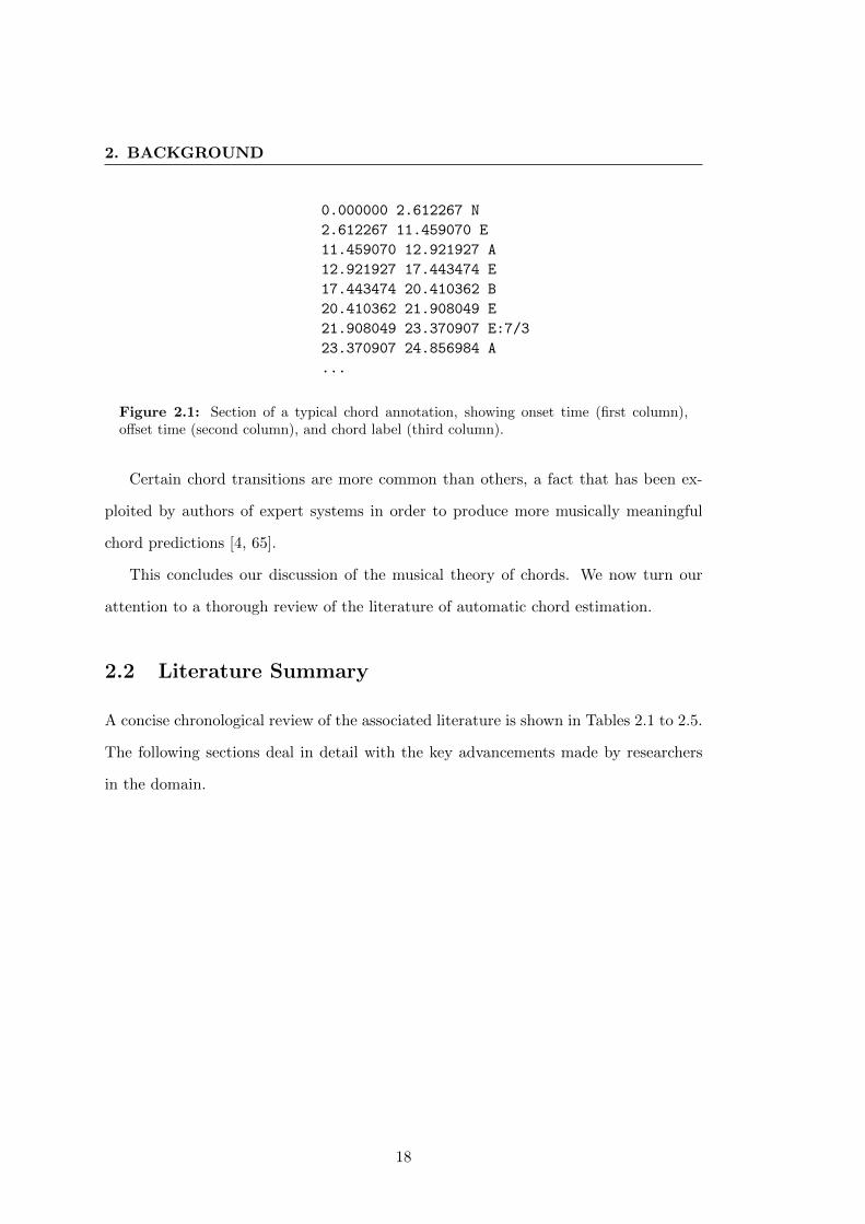
chord progression, a typical example of which is shown in Figure 2.1, where we have
adopted Chris Harte’s suggested syntax for representing chords, where for the most
part chord symbols are represented as rootnote:chordtype/inversion, with some
shorthand notation for major chords (no chord type) and root inversion (no inversion)
[36].
17
2. BACKGROUND
0.000000 2.612267 N
2.612267 11.459070 E
11.459070 12.921927 A
12.921927 17.443474 E
17.443474 20.410362 B
20.410362 21.908049 E
21.908049 23.370907 E:7/3
23.370907 24.856984 A
...
Figure 2.1: Section of a typical chord annotation, showing onset time (first column),offset time (second column), and chord label (third column).
Certain chord transitions are more common than others, a fact that has been ex-
ploited by authors of expert systems in order to produce more musically meaningful
chord predictions [4, 65].
This concludes our discussion of the musical theory of chords. We now turn our
attention to a thorough review of the literature of automatic chord estimation.
2.2 Literature Summary
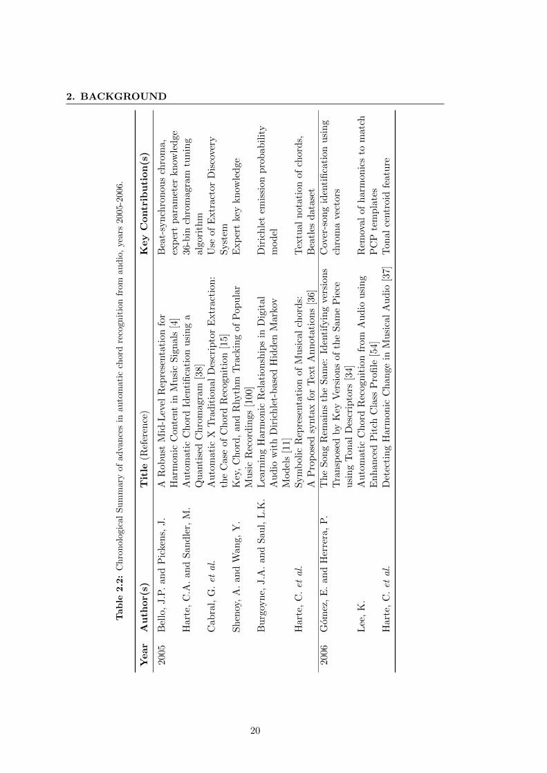
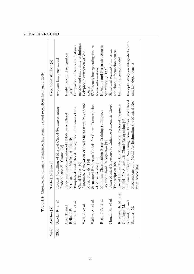
A concise chronological review of the associated literature is shown in Tables 2.1 to 2.5.
The following sections deal in detail with the key advancements made by researchers
in the domain.
18
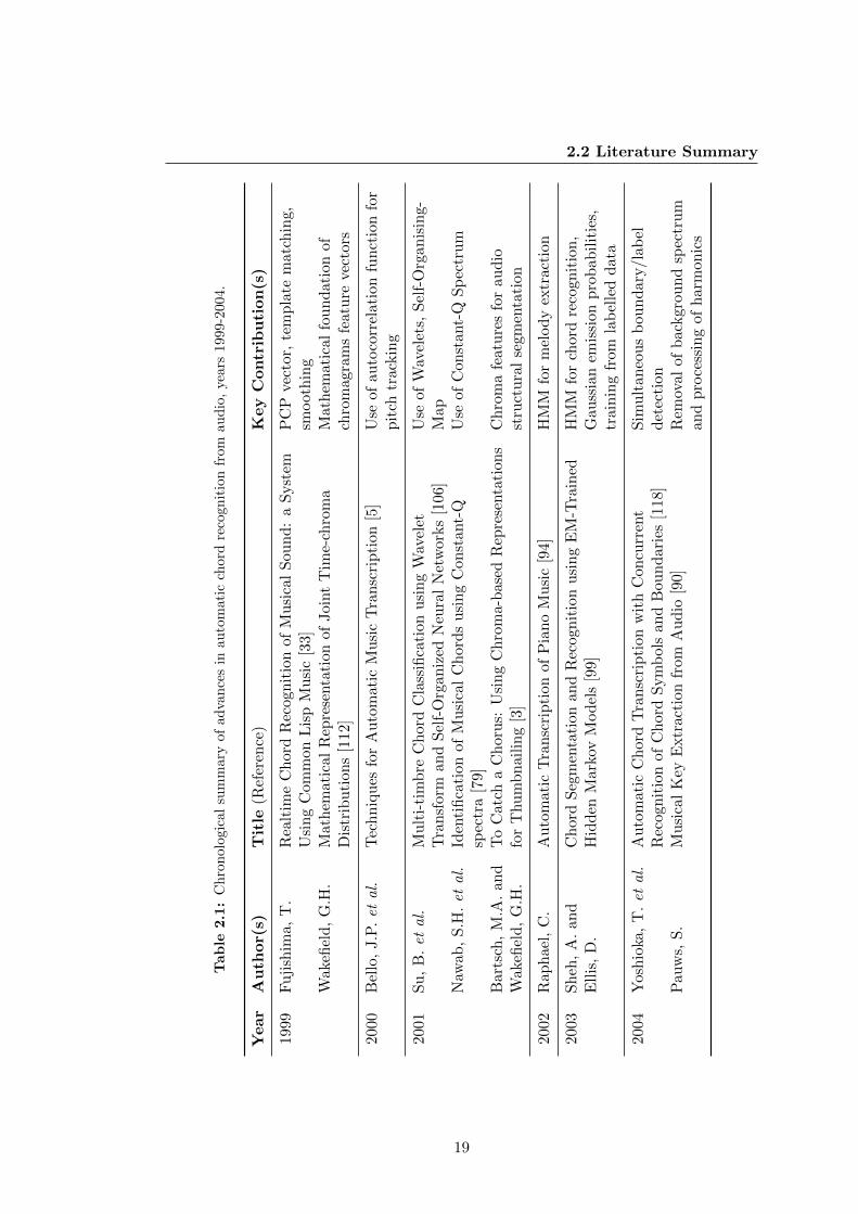
2.2 Literature Summary
Tab
le2.1
:C
hro
nol
ogic
alsu
mm
ary
of
ad
van
ces
inau
tom
ati
cch
ord
reco
gn
itio
nfr
om
au
dio
,ye
ars
1999-2
004.
Year
Au
thor(
s)T
itle
(Ref
eren
ce)
Key
Contr
ibu
tion
(s)
1999
Fu
jish
ima,
T.
Rea
ltim
eC
hor
dR
ecog
nit
ion
ofM
usi
cal
Sou
nd
:a
Syst
emP
CP
vect
or,
tem
pla
tem
atc
hin
g,
Usi
ng
Com
mon
Lis
pM
usi
c[3
3]sm
oot
hin
gW
akefi
eld
,G
.H.
Mat
hem
atic
alR
epre
senta
tion
ofJoi
nt
Tim
e-ch
rom
aM
ath
emat
ical
fou
nd
ati
on
of
Dis
trib
uti
ons
[112
]ch
rom
agra
ms
featu
reve
ctors
2000
Bel
lo,
J.P
.et
al.
Tec
hn
iqu
esfo
rA
uto
mat
icM
usi
cT
ran
scri
pti
on[5
]U
seof
auto
corr
elati
on
fun
ctio
nfo
rp
itch
trac
kin
g
2001
Su,
B.
etal.
Mu
lti-
tim
bre
Ch
ord
Cla
ssifi
cati
onu
sin
gW
avel
etU
seof
Wav
elet
s,S
elf-
Org
an
isin
g-
Tra
nsf
orm
and
Sel
f-O
rgan
ized
Neu
ral
Net
wor
ks
[106
]M
apN
awab
,S
.H.
etal.
Iden
tifi
cati
onof
Mu
sica
lC
hor
ds
usi
ng
Con
stan
t-Q
Use
ofC
onst
ant-
QS
pec
tru
msp
ectr
a[7
9]B
arts
ch,
M.A
.an
dT
oC
atch
aC
hor
us:
Usi
ng
Ch
rom
a-b
ased
Rep
rese
nta
tion
sC
hro
ma
feat
ure
sfo
rau
dio
Wak
efiel
d,
G.H
.fo
rT
hu
mb
nai
lin
g[3
]st
ruct
ura
lse
gmen
tati
on
2002
Rap
hae
l,C
.A
uto
mat
icT
ran
scri
pti
onof
Pia
no
Mu
sic
[94]
HM
Mfo
rm
elod
yex
tract
ion
2003
Sheh
,A
.an
dC
hor
dS
egm
enta
tion
and
Rec
ogn
itio
nu
sin
gE
M-T
rain
edH
MM
for
chor
dre
cogn
itio
n,
Ell
is,
D.
Hid
den
Mar
kov
Mod
els
[99]
Gau
ssia
nem
issi
on
pro
bab
ilit
ies,
trai
nin
gfr
omla
bel
led
data
2004
Yos
hio
ka,
T.
etal.
Au
tom
atic
Ch
ord
Tra
nsc
rip
tion
wit
hC
oncu
rren
tSim
ult
aneo
us
bou
nd
ary
/la
bel
Rec
ogn
itio
nof
Ch
ord
Sym
bol
san
dB
oun
dar
ies
[118
]d
etec
tion
Pau
ws,
S.
Mu
sica
lK
eyE
xtr
acti
onfr
omA
ud
io[9
0]R
emov
alof
bac
kgro
un
dsp
ectr
um
and
pro
cess
ing
of
harm
on
ics
19
2. BACKGROUND
Tab
le2.2
:C
hro
nol
ogic
alS
um
mar
yof
ad
van
ces
inau
tom
ati
cch
ord
reco
gn
itio
nfr
om
au
dio
,ye
ars
2005-2
006.
Year
Au
thor(
s)T
itle
(Ref
eren
ce)
Key
Contr
ibu
tion
(s)
2005
Bel
lo,
J.P
.an
dP
icke
ns,
J.
AR
obu
stM
id-L
evel
Rep
rese
nta
tion
for
Bea
t-sy
nch
ron
ous
chro
ma,
Har
mon
icC
onte
nt
inM
usi
cS
ign
als
[4]
exp
ert
par
amet
erkn
owle
dge
Har
te,
C.A
.an
dS
and
ler,
M.
Au
tom
atic
Ch
ord
Iden
tifi
cati
onu
sin
ga
36-b
inch
rom
agra
mtu
nin
gQ
uan
tise
dC
hro
mag
ram
[38]
algo
rith
mC
abra
l,G
.et
al.
Au
tom
atic
XT
rad
itio
nal
Des
crip
tor
Extr
acti
on:
Use
ofE
xtr
acto
rD
isco
very
the
Cas
eof
Ch
ord
Rec
ogn
itio
n[1
5]S
yst
emS
hen
oy,
A.
and
Wan
g,Y
.K
ey,
Ch
ord
,an
dR
hyth
mT
rack
ing
ofP
opu
lar
Exp
ert
key
know
led
ge
Mu
sic
Rec
ord
ings
[100
]B
urg
oyn
e,J.A
.an
dS
aul,
L.K
.L
earn
ing
Har
mon
icR
elat
ion
ship
sin
Dig
ital
Dir
ich
let
emis
sion
pro
bab
ilit
yA
ud
iow
ith
Dir
ich
let-
bas
edH
idd
enM
arko
vm
od
elM
od
els
[11]
Har
te,
C.
etal.
Sym
bol
icR
epre
senta
tion
ofM
usi
cal
chor
ds:
Tex
tual
not
atio
nof
chord
s,A
Pro
pos
edsy
nta
xfo
rT
ext
An
not
atio
ns
[36]
Bea
tles
dat
aset
2006
Gom
ez,
E.
and
Her
rera
,P
.T
he
Son
gR
emai
ns
the
Sam
e:Id
enti
fyin
gve
rsio
ns
Cov
er-s
ong
iden
tifi
cati
on
usi
ng
Tra
nsp
osed
by
Key
Ver
sion
sof
the
Sam
eP
iece
chro
ma
vect
ors
usi
ng
Ton
alD
escr
ipto
rs[3
4]L
ee,
K.
Au
tom
atic
Ch
ord
Rec
ogn
itio
nfr
omA
ud
iou
sin
gR
emov
alof
har
mon
ics
tom
atc
hE
nh
ance
dP
itch
Cla
ssP
rofi
le[5
4]P
CP
tem
pla
tes
Har
te,
C.
etal.
Det
ecti
ng
Har
mon
icC
han
gein
Mu
sica
lA
ud
io[3
7]T
onal
centr
oid
feat
ure
20

2.2 Literature Summary
Tab
le2.3
:C
hro
nol
ogic
alsu
mm
ary
of
ad
van
ces
inau
tom
ati
cch
ord
reco
gn
itio
nfr
om
au
dio
,ye
ars
2007-2
008.
Year
Au
thor(
s)T
itle
(Ref
eren
ce)
Key
Contr
ibu
tion
(s)
2007
Cat
teau
,B
.et
al.
AP
rob
abil
isti
cF
ram
ewor
kfo
rT
onal
Key
and
Ch
ord
Rig
orou
sfr
am
ework
for
join
tR
ecog
nit
ion
[16]
key
/ch
ord
esti
mati
on
Bu
rgoy
ne,
J.A
.et
al.
AC
ross
-Val
idat
edS
tud
yof
Mod
elli
ng
Str
ateg
ies
for
Cro
ss-v
ali
dati
on
on
Bea
tles
Au
tom
atic
Ch
ord
Rec
ogn
itio
nin
Au
dio
[12]
dat
a,C
ond
itio
nal
Ran
dom
Fie
lds
Pap
adop
oulo
s,H
.an
dL
arge
-Sca
lest
ud
yof
Ch
ord
Est
imat
ion
Alg
orit
hm
sC
omp
arati
vest
ud
yof
exp
ert
Pee
ters
,G
.B
ased
onC
hro
ma
Rep
rese
nta
tion
and
HM
M[8
7]vs.
trai
ned
syst
ems
Zen
z,V
.an
dR
aub
er,
A.
Au
tom
atic
Ch
ord
Det
ecti
onIn
corp
orat
ing
Bea
tC
omb
ined
key,
bea
tan
dch
ord
and
Key
Det
ecti
on[1
19]
mod
elL
ee,
K.
and
Sla
ney
,M
.A
Un
ified
Syst
emfo
rC
hor
dT
ran
scri
pti
onan
dK
eyK
ey-s
pec
ific
HM
Ms,
Extr
acti
onu
sin
gH
idd
enM
arko
vM
od
els
[56]
ton
alce
ntr
oid
inke
yd
etec
tion
2008
Sum
i,K
.et
al.
Au
tom
atic
Ch
ord
Rec
ogn
itio
nb
ased
onP
rob
abil
isti
cIn
tegr
atio
nof
bass
pit
chIn
tegr
atio
nof
Ch
ord
Tra
nsi
tion
and
bas
sP
itch
info
rmat
ion
Est
imat
ion
[107
]P
apad
opou
los,
Han
dS
imu
ltan
eou
sE
stim
atio
nof
Ch
ord
Pro
gres
sion
and
Sim
ult
aneo
us
bea
t/ch
ord
Pee
ters
,G
.D
ownb
eats
from
anA
ud
ioF
ile
[88]
esti
mat
ion
Var
ewyck
,M
.et
al.
AN
ovel
Ch
rom
aR
epre
senta
tion
ofP
olyp
hon
icM
usi
cS
imu
ltan
eou
sb
ack
gro
un
dB
ased
onM
ult
iple
Pit
chT
rack
ing
Tec
hniq
ues
[111
]sp
ectr
a&
harm
on
icre
mov
al
Lee
,K
.A
Syst
emfo
rA
uto
mat
icC
hor
dT
ran
scri
pti
onfr
omA
ud
ioG
enre
-sp
ecifi
cH
MM
sU
sin
gG
enre
-Sp
ecifi
cH
idd
enM
arko
vM
od
els
[55]
Mau
ch,
M.
etal.
AD
iscr
ete
Mix
ture
Mod
elfo
rC
hor
dL
abel
lin
g[6
3]B
ass
chro
magra
m
21
2. BACKGROUND
Tab
le2.4
:C
hro
nol
ogic
alsu
mm
ary
of
ad
van
ces
inau
tom
ati
cch
ord
reco
gn
itio
nfr
om
au
dio
,2009.
Year
Au
thor(
s)T
itle
(Ref
eren
ce)
Key
Contr
ibu
tion
(s)
2009
Sch
olz,
R.
etal.
Rob
ust
Mod
elli
ng
ofM
usi
cal
Ch
ord
Seq
uen
ces
usi
ng
n−
gram
lan
guag
em
od
elP
rob
abil
isti
cN−
Gra
ms
[98]
Ch
o,T
.an
dR
eal-
tim
eIm
ple
men
tati
onof
HM
M-b
ased
Ch
ord
Rea
l-ti
me
chor
dre
cogn
itio
nB
ello
,J.P
.E
stim
atio
nin
Mu
sica
lA
ud
io[1
9]sy
stem
Ou
dre
,L
.et
al.
Tem
pla
te-B
ased
Ch
ord
Rec
ogn
itio
n:
Infl
uen
ceof
the
Com
par
ison
ofte
mp
late
dis
tan
ceC
hor
dT
yp
es[8
6]m
etri
csan
dsm
oot
hin
gte
chn
iques
Wei
l,J.
etal.
Au
tom
atic
Gen
erat
ion
ofL
ead
Sh
eets
from
Pol
yp
hon
icP
olyp
hon
icex
trac
tion
of
lead
Mu
sic
Sig
nal
s[1
14]
shee
tsW
elle
r,A
.et
al.
Str
uct
ure
dP
red
icti
onM
od
els
for
Ch
ord
Tra
nsc
rip
tion
SV
Mst
ruct
,in
corp
orat
ing
futu
reof
Mu
sic
Au
dio
[115
]fr
ame
info
rmat
ion
Ree
d,
J.T
.et
al.
Min
imu
mC
lass
ifica
tion
Err
orT
rain
ing
toIm
pro
ve
Har
mon
ican
dP
ercu
ssiv
eS
ou
rce
Isol
ated
Ch
ord
Rec
ogn
itio
n[9
6]S
epar
atio
n(H
PS
S)
Mau
ch,
M.
etal.
Usi
ng
Mu
sica
lS
truct
ure
toE
nh
ance
Au
tom
atic
Ch
ord
Str
uct
ura
lse
gmen
tati
onas
an
Tra
nsc
rip
tion
[68]
add
itio
nal
info
rmat
ion
sou
rce
Kh
adke
vic
h,
M.
and
Use
ofH
idd
enM
arko
vM
od
els
and
Fac
tore
dL
angu
age
Fac
tore
dla
ngu
age
mod
elO
mol
ogo,
M.
Mod
els
for
Au
tom
atic
Chor
dR
ecog
nit
ion
[45]
Nol
and
,K
.an
dIn
flu
ence
sof
Sig
nal
Pro
cess
ing,
Ton
eP
rofi
les,
and
Ch
ord
In-d
epth
stu
dy
onin
tegra
ted
chord
San
dle
r,M
.P
rogr
essi
ons
ona
Mod
elfo
rE
stim
atin
gth
eM
usi
cal
Key
and
key
dep
end
enci
esfr
omA
ud
io[8
3]
22

2.2 Literature Summary
Tab
le2.5
:C
hro
nol
ogic
alsu
mm
ary
of
ad
van
ces
inau
tom
ati
cch
ord
reco
gn
itio
nfr
om
au
dio
,ye
ars
2010-2
011.
Year
Au
thor(
s)T
itle
(Ref
eren
ce)
Key
Contr
ibu
tion
(s)
2010
Mau
ch,
M.
Au
tom
atic
Ch
ord
Tra
nsc
rip
tion
from
Au
dio
usi
ng
DB
Nm
od
el,
NN
LS
chro
ma
Com
pu
tati
onal
Mod
els
ofM
usi
cal
Con
text
[62]
Ued
a,Y
.et
al.
HM
M-b
ased
app
roac
hfo
rA
uto
mat
icC
hor
dD
etec
tion
HP
SS
wit
had
dit
ion
al
usi
ng
Refi
ned
Aco
ust
icF
eatu
res
[109
]p
ost-
pro
cess
ing
Ch
o,T
.et
al.
Exp
lori
ng
Com
mon
Var
iati
ons
inS
tate
ofth
eA
rtC
hor
dC
omp
aris
on
of
pre
an
dp
ost
-R
ecog
nit
ion
Syst
ems
[21]
filt
erin
gte
chn
iqu
esan
dm
od
els
Kon
z,V
.et
al.
AM
ult
i-p
ersp
ecti
veE
valu
atio
nF
ram
ewor
kfo
rC
hor
dV
isu
alis
atio
nof
evalu
ati
on
Rec
ogn
itio
n[4
9]te
chn
iqu
esM
auch
,M
.et
al.
Lyri
cs-t
o-au
dio
Ali
gnm
ent
and
Ph
rase
-lev
elS
egm
enta
tion
Ch
ord
sequ
ence
sin
lyri
csu
sin
gIn
com
ple
teIn
tern
et-s
tyle
Ch
ord
An
not
atio
ns
[69]
alig
nm
ent
2011
Bu
rgoy
ne,
J.A
.et
al.
An
Exp
ert
Gro
un
dT
ruth
Set
for
Au
dio
Ch
ord
Bil
lboa
rdH
ot
100
data
set
of
Rec
ogn
itio
nan
dM
usi
cA
nal
ysi
s[1
3]ch
ord
ann
ota
tion
sJia
ng,
N.
etal.
An
alysi
ng
Ch
rom
aF
eatu
reT
yp
esfo
rA
uto
mat
edC
omp
aris
on
of
mod
ern
Ch
ord
Rec
ogn
itio
n[4
0]ch
rom
agra
mty
pes
Mac
rae,
R.
and
Gu
itar
Tab
Min
ing,
An
alysi
san
dR
ankin
g[6
0]W
eb-b
ased
chord
lab
els
Dix
on,
S.
Ch
o,T
.an
dA
Fea
ture
Sm
oot
hin
gM
eth
od
for
Chor
dR
ecog
nit
ion
Rec
urr
ence
plo
tfo
rB
ello
,J.P
.U
sing
Rec
urr
ence
Plo
ts[2
0]sm
oot
hin
gY
osh
ii,
K.
and
AV
oca
bu
lary
-Fre
eIn
fin
ity-G
ram
Mod
elfo
rIn
fin
ity-g
ram
lan
gu
age
mod
elG
oto,
M.
Non
-par
amet
ric
Bay
esia
nC
hor
dP
rogr
essi
onA
nal
ysi
s[1
17]
23
2. BACKGROUND
2.3 Feature Extraction
The dominant feature used in automatic chord recognition is the chromagram. We
give a detailed account of the signal processing techniques associated with this feature
vector in this section.
2.3.1 Early Work
The first mention of chromagram feature vectors to our knowledge was by Shepard
[101], where it was noticed that two dimensions, (tone height and chroma) were useful
in explaining how the human auditory system functions. The word chroma is used
to describe pitch class, whereas tone height refers to the octave information. Early
methods of chord prediction were based on polyphonic note transcription [1, 17, 43, 61],
although it was Fujishima [33] who first considered automatic chord recognition as a
task unto itself. His Pitch Class Profile (PCP) feature involved taking a Discrete
Fourier Transform of a segment of the input audio, and from this calculating the power
evolution over a set of frequency bands. Frequencies which were close to each pitch
class (C, C ] , . . . , B) were then collected and collapsed to form a 12–dimensional PCP
vector for each time frame.
For a given input signal, the PCP at each time instance was then compared to
a series of chord templates using either nearest neighbour or weighted sum distance.
Audio input was monophonic piano music and an adventurous 27 chord types were used
as an alphabet. Results approached 94%, measured as the total number of correctly
identified frames divided by total number of frames.
The move from the heuristic PCP vectors to the mathematically-defined chroma-
gram was first rigorously treated by Wakefield [112], who showed that a chromagram
is invariant to octave translation, suggested a method for its calculation and also noted
that chromagrams could be useful for visualisation purposes, demonstrated by an ex-
24
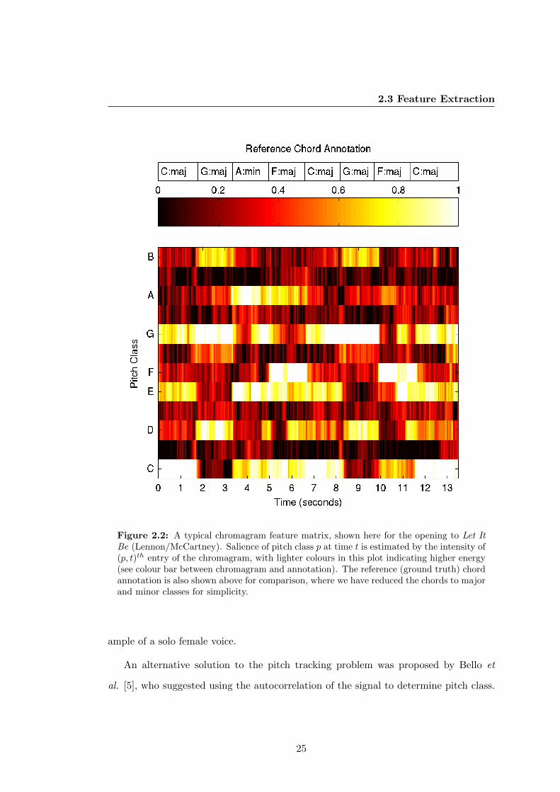
2.3 Feature Extraction
Figure 2.2: A typical chromagram feature matrix, shown here for the opening to Let ItBe (Lennon/McCartney). Salience of pitch class p at time t is estimated by the intensity of(p, t)th entry of the chromagram, with lighter colours in this plot indicating higher energy(see colour bar between chromagram and annotation). The reference (ground truth) chordannotation is also shown above for comparison, where we have reduced the chords to majorand minor classes for simplicity.
ample of a solo female voice.
An alternative solution to the pitch tracking problem was proposed by Bello et
al. [5], who suggested using the autocorrelation of the signal to determine pitch class.
25
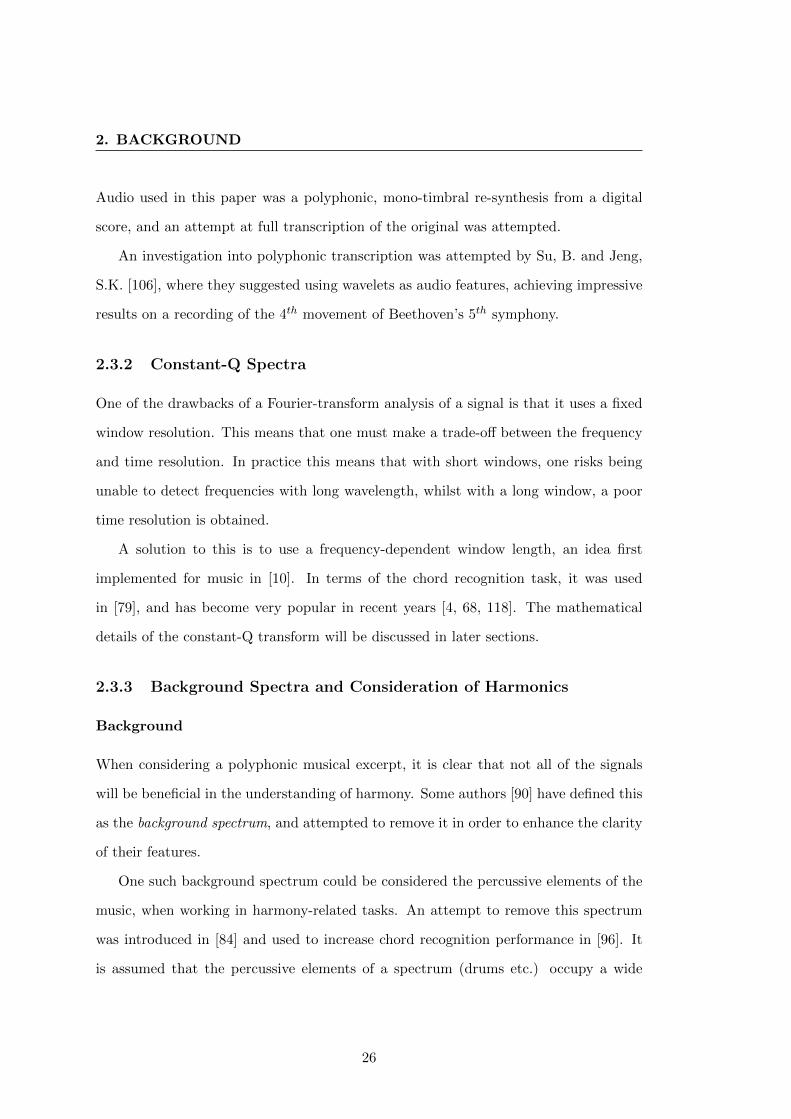
2. BACKGROUND
Audio used in this paper was a polyphonic, mono-timbral re-synthesis from a digital
score, and an attempt at full transcription of the original was attempted.
An investigation into polyphonic transcription was attempted by Su, B. and Jeng,
S.K. [106], where they suggested using wavelets as audio features, achieving impressive
results on a recording of the 4th movement of Beethoven’s 5th symphony.
2.3.2 Constant-Q Spectra
One of the drawbacks of a Fourier-transform analysis of a signal is that it uses a fixed
window resolution. This means that one must make a trade-off between the frequency
and time resolution. In practice this means that with short windows, one risks being
unable to detect frequencies with long wavelength, whilst with a long window, a poor
time resolution is obtained.
A solution to this is to use a frequency-dependent window length, an idea first
implemented for music in [10]. In terms of the chord recognition task, it was used
in [79], and has become very popular in recent years [4, 68, 118]. The mathematical
details of the constant-Q transform will be discussed in later sections.
2.3.3 Background Spectra and Consideration of Harmonics
Background
When considering a polyphonic musical excerpt, it is clear that not all of the signals
will be beneficial in the understanding of harmony. Some authors [90] have defined this
as the background spectrum, and attempted to remove it in order to enhance the clarity
of their features.
One such background spectrum could be considered the percussive elements of the
music, when working in harmony-related tasks. An attempt to remove this spectrum
was introduced in [84] and used to increase chord recognition performance in [96]. It
is assumed that the percussive elements of a spectrum (drums etc.) occupy a wide
26
2.3 Feature Extraction
frequency range but are narrow in the time domain, and harmony (melody, chords,
bassline) conversely. The spectrum is assumed to be a simple sum of percussive and
harmonic material and can be diffused into two constituent spectra, from which the
harmony can be used for chordal analysis.
This process is known as Harmonic Percussive Source Separation (HPSS) and is
shown in [96] and [109] to improve chord recognition significantly. The latter study
also showed that employing post-processing techniques on the chroma including Fourier
transform of chroma vector and increasing the number of states in the HMM by up to
3 offered improvements in recognition rates.
Harmonics
It is known that musical instruments emit not only pure tones f0, but a series of har-
monics at higher frequencies, and subharmonics at lower frequencies. Such harmonics
can easily confuse feature extraction techniques, and some authors have attempted to
remove them in the feature extraction process [54, 65, 87, 90]. An illustrative example
of (sub)harmonics is shown in Figure 2.3.
Figure 2.3: Constant-Q spectrum of a piano playing a single A4 note. Note that, as wellas the fundamental at f0 =A4, there are harmonics at one octave (A5) and one octaveplus a just perfect fifth (E5). Higher harmonics exist but are outside the frequency rangeconsidered here. Notice also the slight presence of a fast-decaying subharmonic at twooctaves down, A2.
27
2. BACKGROUND
A method of removing the background spectra and harmonics simultaneously was
proposed in [111], based on multiple pitch tracking. They note that their new fea-
tures matched chord profiles better than unprocessed chromagrams, a technique which
was also employed by [65]. An alternative to processing the spectrum is to introduce
harmonics into the modelling strategy, a concept we will discuss in section 2.4.
2.3.4 Tuning Compensation
In 2003, Sheh and Ellis [99] identified that some popular music tracks are not tuned to
standard pitch A4 = 440 Hz, meaning that for these songs, chromagram features may
misrepresent the salient pitch classes. To counteract this, they constructed finer-grained
chromagram feature vectors of 24, instead of 12, dimensions, allowing for flexibility in
the tuning of the piece. Harte [38] introduced a tuning algorithm which computed a
chromagram feature matrix over a finer granularity of 3 frequency bands per semitone,
and searched for the sub-band which contained the most energy. This was chosen as
the tuning of the piece and the actual saliences inferred by interpolation. This method
also used by Bello and Pickens [4] and in Harte’s own work [37].
2.3.5 Smoothing/Beat Synchronisation
It was noticed by Fujishima [33] that using instantaneous chroma features did not
provide musically meaningful predictions, owing to transients meaning predicted chords
were changing too frequently. As an initial solution, some smoothing of the PCP
vectors was introduced. This heuristic was repeated by other authors using template-
based chord recognition systems (see section 2.4), including [52]. In [4], the concept
of exploiting the fact that chords are relatively stable between beats [35] was used to
create beat-synchronous chromagrams, where the time resolution is reduced to that of
the main pulse. This method was shown to be superior in terms of recognition rate,
but also had the advantage that the overall computation cost is also reduced, owing to
28

2.3 Feature Extraction
the total number of frames typically being reduced. Examples of smoothing techniques
are shown in Figure 2.4.
(a) No Smoothing (b) Median smoothing (c) Beat-synchronisation
Figure 2.4: Smoothing techniques for chromagram features. In 2.4a, we see a standardchromagram feature. Figure 2.4b shows a median filter over 20 frames, 2.4c shows a beat-synchronised chromagram.
Popular methods of smoothing chroma features are to take the mean [4] or median
[65] salience of each of the pitch classes between beats. In more recent work, [20]
recurrence plots were used within similar segments and shown to be superior to beat
synchronisation or mean/median filtering.
Papadopoulus and Peeters [88] noted that a simultaneous estimate of beats led to
an improvement in chords and vice-versa, supporting an argument that an integrated
model of harmony and rhythm may offer improved performance in both tasks. A
comparative study of post-processing techniques was conducted in [21], where they
also compared different pre-filtering and modelling techniques.
2.3.6 Tonal Centroid Vectors
An interesting departure from traditional chromagrams was presented in [37], notably
a transform of the chromagram known as the Tonal Centroid feature. This feature
is based on the idea that close harmonic relationships such as perfect fifths and ma-
29
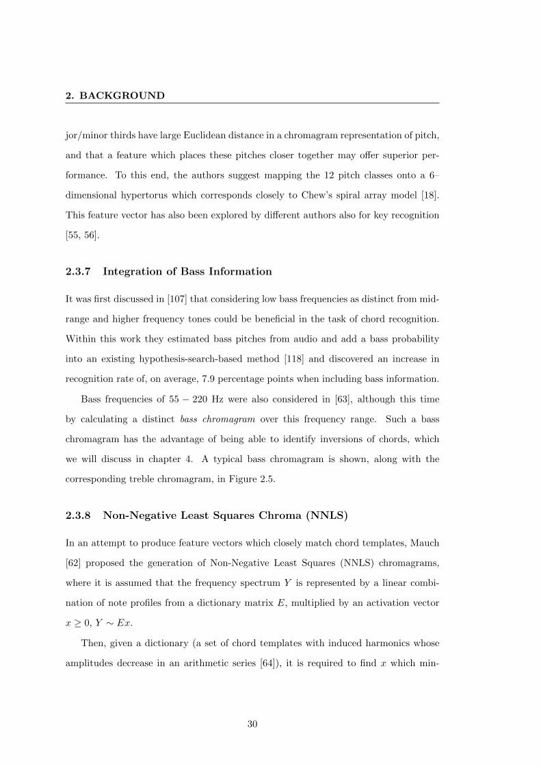
2. BACKGROUND
jor/minor thirds have large Euclidean distance in a chromagram representation of pitch,
and that a feature which places these pitches closer together may offer superior per-
formance. To this end, the authors suggest mapping the 12 pitch classes onto a 6–
dimensional hypertorus which corresponds closely to Chew’s spiral array model [18].
This feature vector has also been explored by different authors also for key recognition
[55, 56].
2.3.7 Integration of Bass Information
It was first discussed in [107] that considering low bass frequencies as distinct from mid-
range and higher frequency tones could be beneficial in the task of chord recognition.
Within this work they estimated bass pitches from audio and add a bass probability
into an existing hypothesis-search-based method [118] and discovered an increase in
recognition rate of, on average, 7.9 percentage points when including bass information.
Bass frequencies of 55 − 220 Hz were also considered in [63], although this time
by calculating a distinct bass chromagram over this frequency range. Such a bass
chromagram has the advantage of being able to identify inversions of chords, which
we will discuss in chapter 4. A typical bass chromagram is shown, along with the
corresponding treble chromagram, in Figure 2.5.
2.3.8 Non-Negative Least Squares Chroma (NNLS)
In an attempt to produce feature vectors which closely match chord templates, Mauch
[62] proposed the generation of Non-Negative Least Squares (NNLS) chromagrams,
where it is assumed that the frequency spectrum Y is represented by a linear combi-
nation of note profiles from a dictionary matrix E, multiplied by an activation vector
x ≥ 0, Y ∼ Ex.
Then, given a dictionary (a set of chord templates with induced harmonics whose
amplitudes decrease in an arithmetic series [64]), it is required to find x which min-
30
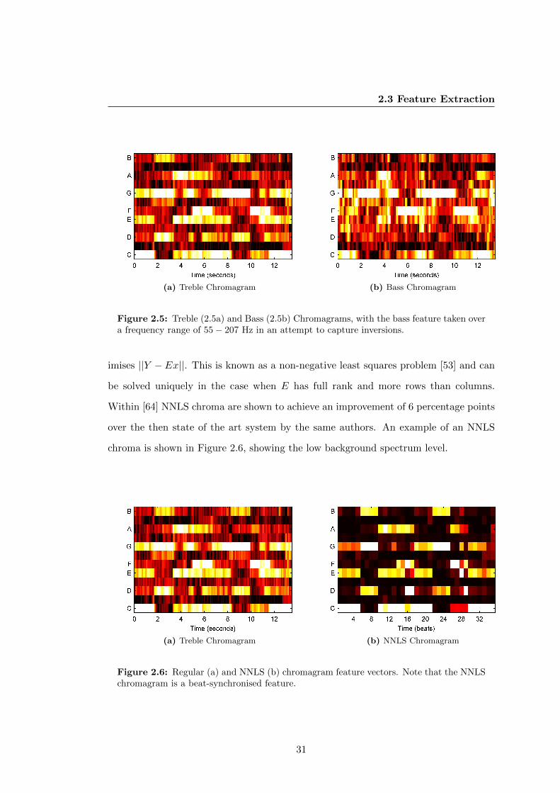
2.3 Feature Extraction
(a) Treble Chromagram (b) Bass Chromagram
Figure 2.5: Treble (2.5a) and Bass (2.5b) Chromagrams, with the bass feature taken overa frequency range of 55− 207 Hz in an attempt to capture inversions.
imises ||Y −Ex||. This is known as a non-negative least squares problem [53] and can
be solved uniquely in the case when E has full rank and more rows than columns.
Within [64] NNLS chroma are shown to achieve an improvement of 6 percentage points
over the then state of the art system by the same authors. An example of an NNLS
chroma is shown in Figure 2.6, showing the low background spectrum level.
(a) Treble Chromagram (b) NNLS Chromagram
Figure 2.6: Regular (a) and NNLS (b) chromagram feature vectors. Note that the NNLSchromagram is a beat-synchronised feature.
31

2. BACKGROUND
A comparative study of modern chromagram types was also conducted in [40],
and later developed into a toolkit for research purposes [78]. We have seen many
techniques for chromagram computation in this Section. Some of these (constant-Q,
tuning, beat-synchronisation, bass chromagrams) will be used in the design of our
features (see Chapter 3, whilst others (Tonal centroid vectors) will not. The author
decided against using tonal centroid vectors as they are low-dimensional and therefore
suited to situations with less training data, and also less easily interpreted than a
chromagram representation.
2.4 Modelling Strategies
In this section, we review the next major problem in the domain of chord recognition:
assigning labels to chromagram (or related feature) frames. We begin with a discussion
of simple pattern-matching techniques.
2.4.1 Template Matching
Template matching involves comparing feature vectors against the known distribution
of notes in a chord. Typically, a 12–dimensional chromagram is compared to a binary
vector containing ones where a trial chord has notes present. For example, the template
for a C:major chord would be [1 0 0 0 1 0 0 1 0 0 0 0]. Each frame of the chromagram is
compared to a set of templates, and the template with minimal distance to the chroma
is output as the label for this frame (see Figure 2.7).
This technique was first proposed by Fujishima, where he used either the nearest
neighbour template or a weighted sum [33] as a distance metric between templates and
chroma frames. Similarly, this technique was used by Cabral and collaborators [15]
who compared it to the Extractor Discovery System (EDS) software to classify chords
in Bossa Nova songs.
32
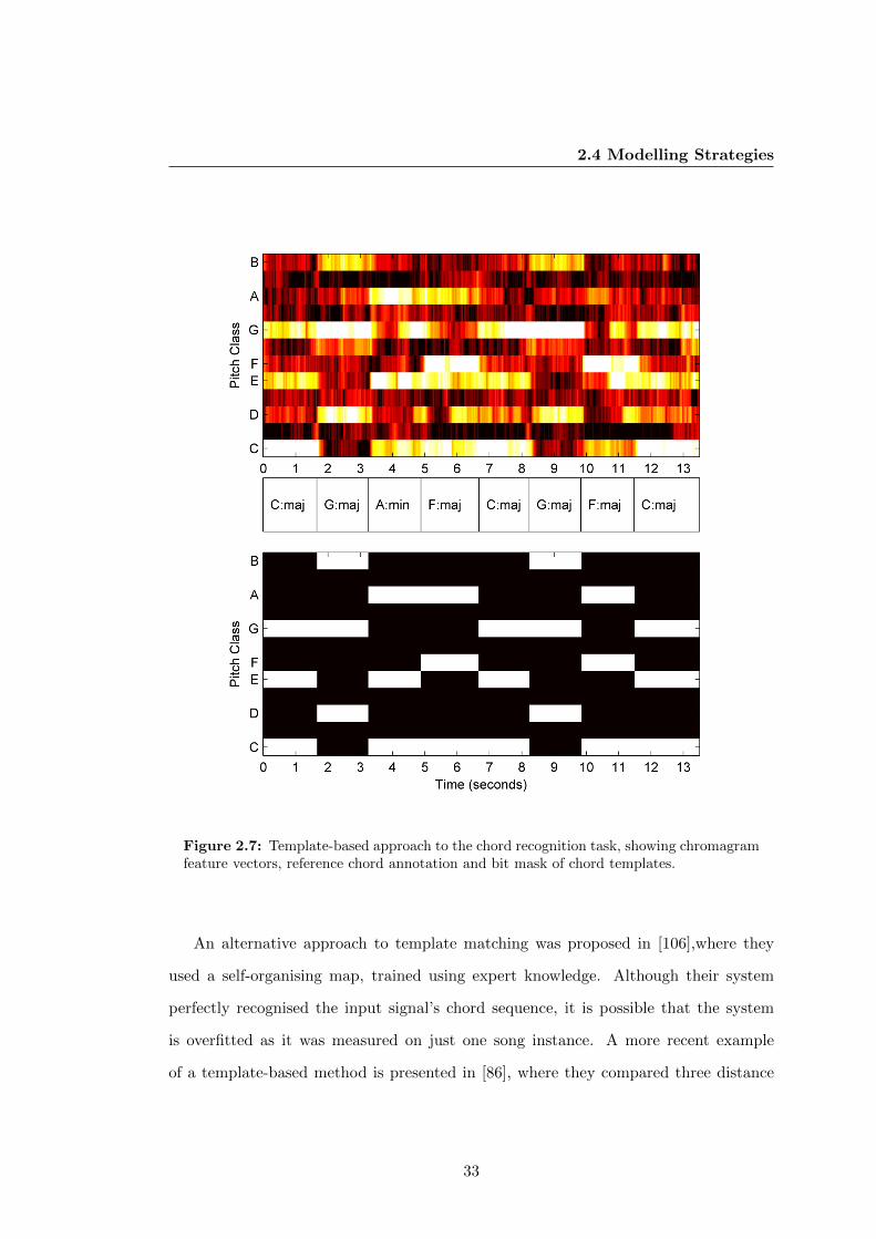
2.4 Modelling Strategies
Figure 2.7: Template-based approach to the chord recognition task, showing chromagramfeature vectors, reference chord annotation and bit mask of chord templates.
An alternative approach to template matching was proposed in [106],where they
used a self-organising map, trained using expert knowledge. Although their system
perfectly recognised the input signal’s chord sequence, it is possible that the system
is overfitted as it was measured on just one song instance. A more recent example
of a template-based method is presented in [86], where they compared three distance
33
2. BACKGROUND
measures and two post-processing smoothing types and found that Kullback-Leibler
divergence [52] and median filtering offered an improvement over the then state of the
art. Further examples of template-based chord recognition systems can be found in
[85].
2.4.2 Hidden Markov Models
Individual pattern matching techniques such as template matching fail to model the
continuous nature of chord sequences. This can be combated by either using smoothing
methods as seen in 2.3 or by including duration in the underlying model. One of the
most common ways of incorporating smoothness in the model is to use a Hidden Markov
Model (HMM, defined formally in Section 2.7).
An HMM models a time-varying process where one witnesses a sequence of observed
variables coming from a corresponding sequence of hidden nodes, and can be used to
formalize a probability distribution jointly for the chromagram feature vectors and the
chord annotations of a song. In this model, the chords are modelled as a first-order
Markovian process. Furthermore, given a chord, the feature vector in the corresponding
time window is assumed to be independent of all other variables in the model. The
chords are commonly referred to as the hidden variables and the chromagram feature
vectors as the observed variables, as the chords are typically unknown and to be inferred
from the given chromagram feature vectors in the chord recognition task. See Figure
2.8 for a visual representation of an HMM.
Arrows in Figure 2.8 refer to the inherent conditional probabilities of the HMM
architecture. Horizontal arrows represent the probability of one chord following another
(the transition probabilities), vertical arrows the probability of a chord emitting a
particular chromagram (the emission probabilities). Learning these probabilities may
either be done using expert knowledge or using labelled training data.
Although HMMs are very common in the domain of speech recognition [92], we
34
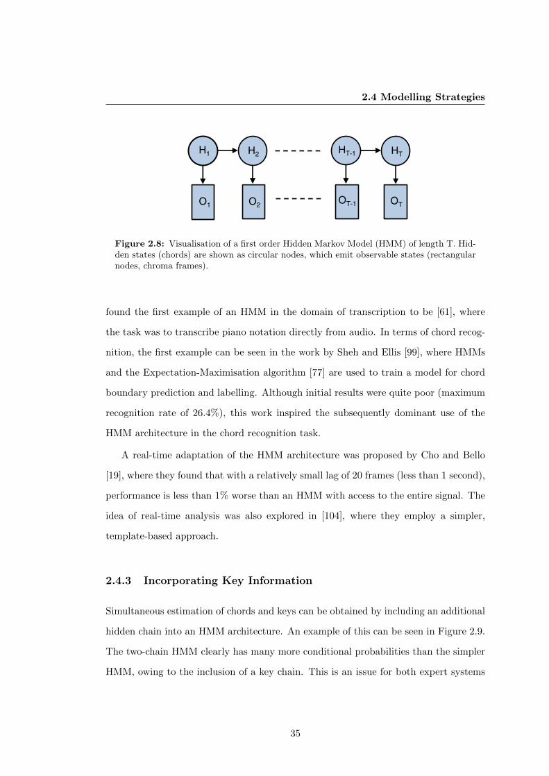
2.4 Modelling Strategies
H1 H2 HT-1
O1 O2 OT-1 OT
HT
Figure 2.8: Visualisation of a first order Hidden Markov Model (HMM) of length T. Hid-den states (chords) are shown as circular nodes, which emit observable states (rectangularnodes, chroma frames).
found the first example of an HMM in the domain of transcription to be [61], where
the task was to transcribe piano notation directly from audio. In terms of chord recog-
nition, the first example can be seen in the work by Sheh and Ellis [99], where HMMs
and the Expectation-Maximisation algorithm [77] are used to train a model for chord
boundary prediction and labelling. Although initial results were quite poor (maximum
recognition rate of 26.4%), this work inspired the subsequently dominant use of the
HMM architecture in the chord recognition task.
A real-time adaptation of the HMM architecture was proposed by Cho and Bello
[19], where they found that with a relatively small lag of 20 frames (less than 1 second),
performance is less than 1% worse than an HMM with access to the entire signal. The
idea of real-time analysis was also explored in [104], where they employ a simpler,
template-based approach.
2.4.3 Incorporating Key Information
Simultaneous estimation of chords and keys can be obtained by including an additional
hidden chain into an HMM architecture. An example of this can be seen in Figure 2.9.
The two-chain HMM clearly has many more conditional probabilities than the simpler
HMM, owing to the inclusion of a key chain. This is an issue for both expert systems
35
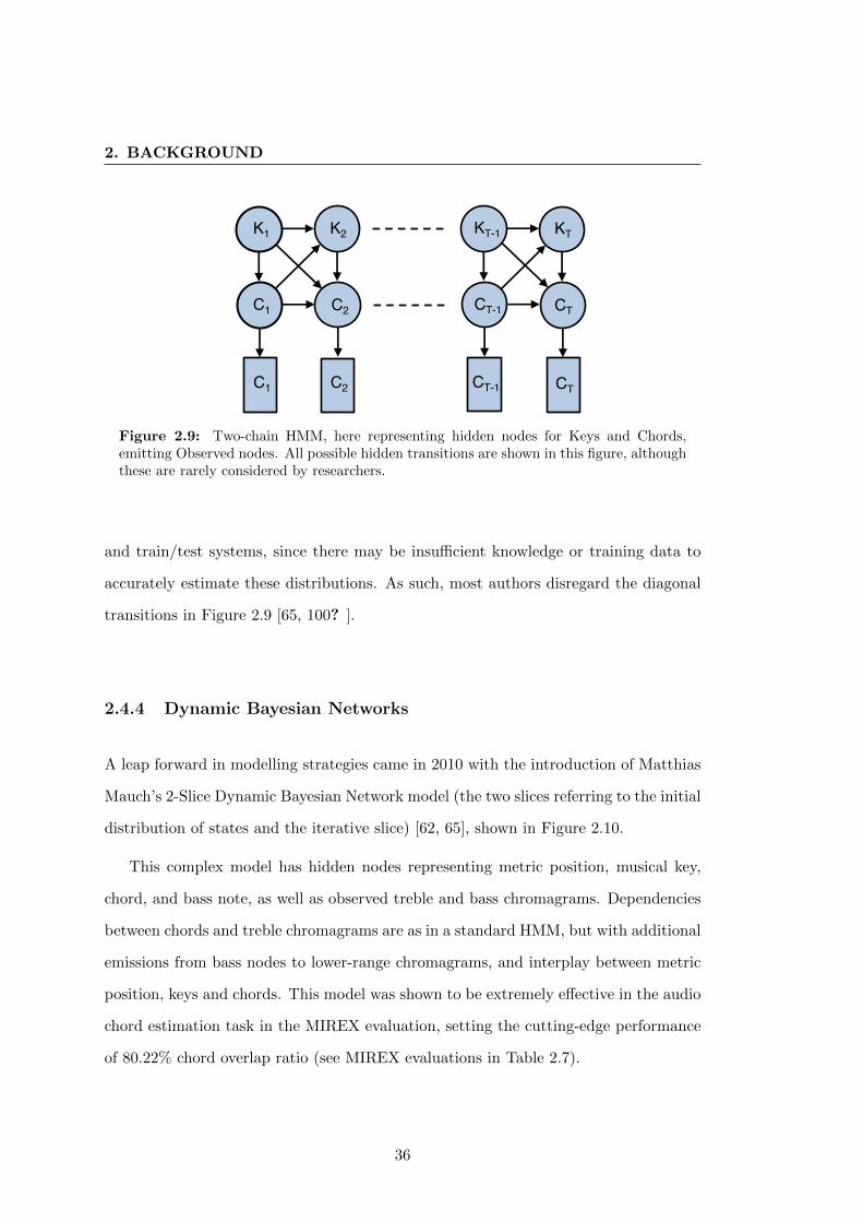
2. BACKGROUND
K1 K2 KT-1 KT
C1 C2 CT-1 CT
C1 C2 CT-1 CT
Figure 2.9: Two-chain HMM, here representing hidden nodes for Keys and Chords,emitting Observed nodes. All possible hidden transitions are shown in this figure, althoughthese are rarely considered by researchers.
and train/test systems, since there may be insufficient knowledge or training data to
accurately estimate these distributions. As such, most authors disregard the diagonal
transitions in Figure 2.9 [65, 100? ].
2.4.4 Dynamic Bayesian Networks
A leap forward in modelling strategies came in 2010 with the introduction of Matthias
Mauch’s 2-Slice Dynamic Bayesian Network model (the two slices referring to the initial
distribution of states and the iterative slice) [62, 65], shown in Figure 2.10.
This complex model has hidden nodes representing metric position, musical key,
chord, and bass note, as well as observed treble and bass chromagrams. Dependencies
between chords and treble chromagrams are as in a standard HMM, but with additional
emissions from bass nodes to lower-range chromagrams, and interplay between metric
position, keys and chords. This model was shown to be extremely effective in the audio
chord estimation task in the MIREX evaluation, setting the cutting-edge performance
of 80.22% chord overlap ratio (see MIREX evaluations in Table 2.7).
36
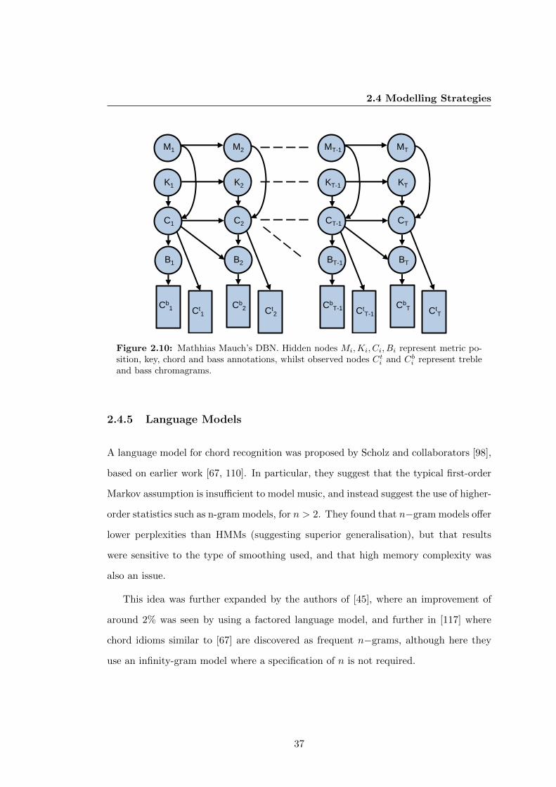
2.4 Modelling Strategies
CT-1
CbT-1 Ct
T-1
BT-1
KT-1
MT-1
CbT Ct
T
CT
BT
KT
MT
C1
Cb1 Ct
1
B1
K1
M1
Cb2 Ct
2
C2
B2
K2
M2
Figure 2.10: Mathhias Mauch’s DBN. Hidden nodes Mi,Ki, Ci, Bi represent metric po-sition, key, chord and bass annotations, whilst observed nodes Ct
i and Cbi represent treble
and bass chromagrams.
2.4.5 Language Models
A language model for chord recognition was proposed by Scholz and collaborators [98],
based on earlier work [67, 110]. In particular, they suggest that the typical first-order
Markov assumption is insufficient to model music, and instead suggest the use of higher-
order statistics such as n-gram models, for n > 2. They found that n−gram models offer
lower perplexities than HMMs (suggesting superior generalisation), but that results
were sensitive to the type of smoothing used, and that high memory complexity was
also an issue.
This idea was further expanded by the authors of [45], where an improvement of
around 2% was seen by using a factored language model, and further in [117] where
chord idioms similar to [67] are discovered as frequent n−grams, although here they
use an infinity-gram model where a specification of n is not required.
37
2. BACKGROUND
2.4.6 Discriminative Models
The authors of [12] suggest that the commonly-used Hidden Markov Model is not appro-
priate for use in the chord recognition task, preferring instead the use of a Conditional
Random Field (CRF), a type of discriminative model (as opposed to a generative model
such as an HMM).
During decoding, an HMM seeks to maximise the overall joint over the chords
and feature vectors P (X,Y). However, for a given song example the observation is
always fixed, so it may be more sensible to model the conditional P (Y|X), relaxing
the necessity for the components of the observations to be conditionally independent.
In this way, discriminative models attempt to achieve accurate input (chromagram) to
output (chord sequence) mappings.
An additional potential benefit to this modelling strategy is that one may address
the balance between, for example, the hidden and observation probabilities, or take into
account more than one frame (or indeed an entire chromagram) in labelling a particular
frame. This last approach was explored in [115], where the recently developed SVM-
struct algorithm was used as opposed to CRF, in addition to incorporating information
about future chromagram frames to show an improvement over a standard HMM.
2.4.7 Genre-Specific Models
Lee [57] has suggested that training a single model on a wide range of genres may lead
to poor generalisation, an idea which was expanded on in [55], where they found that if
genre information was given (for a range of 6 genres), performance increased almost 10
percentage points. Also, they note that their method can be used to identify genre in
a probabilistic way, by simply testing all genre-specific models and choosing the model
with largest likelihood. Although their classes were very unbalanced, they correctly
identified 24/28 songs as rock (85.71%).
38

2.5 Model Training and Datasets
2.4.8 Emission Probabilities
When considering the probability of a chord emitting a feature vector in graphical
models such as [63, 74, 99] one must specify a probability distribution. A common
method for doing this is to use a 12–dimensional Gaussian distribution, i.e the proba-
bility of a chord c emitting a chromagram frame x is set as P (x|c) ∼ N(µ,Σ), with µ a
12–dimensional mean vector for each chord and Σ a covariance matrix for each chord.
One may then estimate µ and Σ from data or expert knowledge and infer the emission
probability for a (chord, chroma) pair.
This technique has been very widely used in the literature (see, for example [4,
40, 45, 99]). A slightly more sophisticated emission model is to consider a mixture of
Gaussians, instead of one per chord. This has been explored in, for example, [20, 96,
107].
A different emission model was proposed in [11], that of a Dirichlet model. Given
a chromagram with pitch classes p = {c1, . . . , c12}, each with probability {p1, . . . , p12}
and∑12
i=1 pi = 1, pi > 0 ∀i, a dirichlet distribution with parameters u = {u1, . . . , u12}
is defined as
P (x|c) =1
Nu
12∏i=1
piui−1 (2.5)
where Nu is a normalisation term. Thus, a Dirichlet distribution is a distribution over
numbers which sum to one, and a good candidate for a chromagram feature vector. This
emission model was implemented in the chord recognition task in [12], with encouraging
results.
2.5 Model Training and Datasets
As mentioned previously, graphical models such as HMMs, two-chain HMMs, and Dy-
namic Bayesian Networks require training in order to infer the parameters necessary
39
2. BACKGROUND
to predict the chords to an unlabelled song. Various ways of training such models are
discussed in this section, beginning with expert knowledge.
2.5.1 Expert Knowledge
In early chord recognition work, when training data was very scarce, an HMM was used
in chord recognition by the authors of [4], where initial parameter settings such as the
state transition probabilities, mean and covariance matrices were set heuristically by
hand, and then enhanced using the Expectation-Maximisation algorithm [92].
A large amount of knowledge was injected into Shenoy and Wang’s key/chord/rhythm
extraction algorithm [100]. For example, they set high weights to primary chords in
each key (tonic, dominant and subdominant), additionally specifying that if the first
three beats of a bar are a single chord, the last beat must also be this chord, and that
chords non-diatonic to the current key are not permissible. They notice that by making
a rough estimate of the chord sequence, they were able to extract the global key of a
piece (assuming no modulations) with high accuracy (28/30 song examples). Using this
key, chord estimation accuracy increased by an absolute 15.07%.
Expert tuning of key-chord dependencies was also explored in [16], following the
theory set out in Lerdahl [58]. A study of expert knowledge versus training was con-
ducted in [87], where they compared expert setting of Gaussian emissions and transition
probabilities, and found that expert tuning with representation of harmonics performed
the best. However, they only used 110 songs in the evaluation, and it is possible that
with the additional data now available, a trained approach may be superior.
Mauch and Dixon [63] also define chord transitions by hand, in the previously men-
tioned work by defining an expert transition probability matrix which has a preference
for chords to remain stable.
40
2.5 Model Training and Datasets
2.5.2 Learning from Fully-labelled Datasets
An early dataset for a many-song corpus was presented in [99], containing 20 early
works by the pop group The Beatles. Within, chord labels were annotated by hand
and manually aligned to the audio, for use in a chord recognition task. This was ex-
panded in work by Harte et al. [36], where they introduced a syntax for annotating
chords in flat text, which has since become standard practice, and also increased the
number of annotated songs by this group to 180.
A small set of 35 popular music songs was studied by Veronika Zenz and Andreas
Rauber [119], where they incorporated beat and key information into a heuristic method
for determining chord labels and boundaries. More recently, the Structural Analysis of
Large Amounts of Music Information (SALAMI) project [13, 102] announced a large
amount of partially-labelled chord sequences and structural segmentations, amongst
other meta data. A total of 869 songs appearing in the Billboard Hot 100 were anno-
tated at the structure level in Chris Harte’s format.
We define sets above as Ground Truth datasets (collections of time-aligned chord
sequences curated by an expert in a format similar to Figure 2.1.) Given a set of such
songs, one may attempt to learn model parameters and probability distributions from
these data. For instance, one may collect chromagrams for all time instances when
a C:maj chord is played, and learn how such a chord ‘sounds’, given an appropriate
emission probability model. Similarly for hidden features, one may count transitions
between chords and learn common chord transitions (as well as typical chord durations).
This method has become extremely popular in recent years as the number of training
examples has increased (see, for example [20, 40, 117? ]).
41
2. BACKGROUND
2.5.3 Learning from Partially-labelled Datasets
In addition to our previously published work [72, 74], Macrae and Dixon have been
exploring readily-available chord labels from the internet [2, 59] for ranking, musical
education, and score following. Such annotations are noisy and potentially difficult to
use, but offer much in terms of volume of data available and are very widely used by
musicians. For example, it was found in [60] that the most popular tab websites have
over 2.5 million visitors, whilst sheet music and MIDI sites have under 500,000 and
20,000 visitors respectively.
A large number of examples of each song are available on such sites, which we refer
to as redundancies of tabs. For example, the authors of [60] found 24,746 redundancies
for songs by The Beatles, or an average of 137.5 tabs per song, whilst in [72] it was
found that there were tabs for over 75,000 unique songs. The possibility of using such
data to train a chord recognition model will be investigated in chapter 5.
2.6 Evaluation Strategies
Given the output of a chord recognition system and a known and trusted ground truth,
methods of performance evaluation are required to compare algorithms and define the
state of the art. We discuss strategies for this in the current section.
2.6.1 Relative Correct Overlap
Fujishima [33] first introduced the concept of the ‘relative correct overlap’ measure for
evaluating chord recognition performance, defined as
RCO =| correctly identified frames |
| total frames |(×100%) (2.6)
42
2.6 Evaluation Strategies
When dealing with a collection of more than one song, one may either average the per-
formances over each song, or concatenate all frames together and measure performance
on this collection (mirco vs. macro average). The former treats each song equally
independent of song length, whilst the latter gives more weight to longer songs.
Mathematically, suppose we have a ground truth and prediction for i = {1, . . . , n, . . . N}
songs, denoted by G = {G1, . . . , Gn, . . . , GN} and P = {P 1, . . . , Pn, . . . , PN}. Suppose
also that the nth ground truth and prediction each have ni frames. Then, given a
distance d(c1, c2) between two chords we may define
ARCO =1
N
N∑i=1
1
ni
ni∑f=1
d(Gif , P
if ) (2.7)
as the Average Relative Correct Overlap, and
TRCO =
(N∑i=1
ni
)−1 N∑i=1
ni∑f=1
d(Gif , P
if ) (2.8)
as the Total Relative Correct Overlap. The most common distance measure is to filter
all chords in the ground truth and prediction according to a pre-defined alphabet and
sample per predicted beat, and set d(Gif , P
if ) = 1 ⇐⇒ (Gi
f = P if ).
2.6.2 Chord Detail
An issue in the task of chord recognition is the level of detail on which to model and
evaluate. Clearly, there are many permissible chords available in music, and we cannot
hope to correctly classify them all.
Considering chords which do not exceed 1 octave, there are 12 pitch classes which
may or may not be present, leaving us with 212 possible chords. Such a chord alphabet
is clearly prohibitive for modelling (owing to the computational complexity) and also
poses issues in terms of evaluation. For these reasons, researchers in the field have
43
2. BACKGROUND
reduced their reference chord annotations to a subset of workable alphabet.
In early work, Fujishima considered 27 chord types, including advanced examples
such as A:(1,3,]5,7)/G. A step forward to a more workable alphabet came in 2003,
where Sheh and Ellis [99] considered 7 chord types (maj,min,maj7,min7,dom7,aug,dim),
although other authors have explored using just the 4 main triads maj,min,aug and
dim [12, 118]. Suspended chords were identified in [63, 107], the latter study addition-
ally containing a ‘no chord’ symbol for silence, speaking or other times when no chord
can be assigned. A large chord alphabet of 10 chord types including inversions were
recognised by Mauch [65]. However, by far the most common chord alphabet is the set
of major and minor chords in addition to a ‘no chord’ symbol, which we collectively
denote as minmaj [54, 87].
2.6.3 Cross-validation Schemes
For systems which rely on training to learn model parameters, it is worth noting that
choosing ‘fair’ splits from fully-labelled sets is non-trivial. One notable effect is that
musical content can be quite different between albums, for a given artist. This is known
as the Album Effect and is a known issue in artist identification [46, 116]. In this case
it is shown that identification of artists is more challenging when the test set consists
of songs from an album not in the training set.
For ACE, the problem is less well-studied, although, although intuitively the same
property should hold. However, informal experiments by the author revealed that
training on a fixed percentage of each album and testing on the remainder resulted in
lower test set performance. Despite this, the MIREX evaluations are conducted in this
manner, which we emulate to make results comparable.
44
2.6 Evaluation Strategies
2.6.4 The Music Information Retrieval Evaluation eXchange (MIREX)
Since 2008, Audio Chord Estimation algorithms have been compared in an annual evalu-
ation held in conjunction with the International Society for Music Information Retrieval
conference1. Authors submit algorithms which are tested on a (known) dataset of au-
dio and ground truths and results compared. We present a summary of the algorithms
submitted in Tables 2.6 - 2.7.
1http://www.music-ir.org/mirex/wiki/MIREX_HOME
45
2. BACKGROUND
Tab
le2.6
:M
IRE
XS
yst
ems
from
2008
-200
9,so
rted
inea
chyea
rby
Tota
lR
elati
veC
orr
ect
Over
lap
inth
em
erged
evalu
ati
on
(con
fusi
ng
par
alle
lm
ajo
r/m
inor
chor
ds
not
con
sid
ered
an
erro
r).
Th
eb
est-
per
form
ing
pre
train
ed/ex
per
tsy
stem
sare
un
der
lin
ed,
bes
ttr
ain
/tes
tsy
stem
sar
ein
bold
face.
Syst
ems
wh
ere
no
data
isav
ail
ab
leare
show
nby
ad
ash
(-).
Perf
orm
an
ce
Year
Cate
gory
Su
b.
Au
thor(
s)A
pp
roach
Un
mer
ged
Mer
ged
2008
Tra
in/T
est
UM
SY
.U
chiy
ama
etal.
Ch
rom
a,H
MM
0.7
20.7
7D
ED
.E
llis
Ch
rom
a,H
MM
0.66
0.7
0W
D2
J.
Wei
lT
onal
Cen
troi
d,
HM
M0.
660.7
0P
retr
ain
edB
PJ.
P.
Bel
lo,
J.
Pic
ken
sC
hro
ma,
HM
M0.
660.6
9M
MM
.M
ehn
ert
Cir
cula
rP
itch
Sp
ace,
HM
M0.
650.6
8R
KM
.R
yyn
nen
,A
.K
lap
uri
Bas
s/T
reb
leC
hro
ma,
HM
M0.
640.6
9P
PH
.Pap
adop
oulo
s,G
.P
eete
rsC
hro
ma,
HM
M0.
630.6
6T
rain
/tes
tK
OM
.K
had
kev
ich
,M
.O
mol
ogo
Ch
rom
a,H
MM
0.62
0.6
5W
D1
J.
Wei
lT
onal
Cen
troi
d,
HM
M0.
600.6
6P
retr
ain
edK
L2
K.L
ee-
0.59
0.6
5T
rain
/tes
tK
LK
.L
ee-
0.58
0.6
5P
retr
ain
edK
L1
K.L
ee-
0.56
0.6
0T
rain
/tes
tZ
LX
.Jh
ang,
C.
Las
hC
hro
ma,
HM
M0.
360.4
6
2009
Tra
in/T
est
WE
J4
A.
Wel
ler
etal.
Ch
rom
a,S
VM
stru
ct+
0.7
42
0.7
77
WE
J2
A.
Wel
ler
etal.
Ch
rom
a,S
VM
stru
ct0.
723
0.7
62
WE
J3
A.
Wel
ler
etal.
Ch
rom
a,M
ax-γ
0.72
30.7
60
Exp
ert
MD
M.
Mau
chet
al.
Bas
s/T
reb
leC
hro
ma,
DB
N0.
712
0.7
48
Pre
trai
ned
OG
F2
L.
Ou
dre
etal.
Ch
rom
a,T
emp
late
0.71
10.7
77
KO
2M
.K
had
kevic
h&
M.
Om
olog
oC
hro
ma,
HM
M0.
708
0.7
41
OG
F1
L.
Ou
dre
etal.
Ch
rom
a,T
emp
late
0.70
60.7
70
Tra
in/T
est
WE
J1
A.
Wel
ler
etal.
Ch
rom
a,H
MM
0.70
40.7
43
RU
SU
SL
J.T
.Ree
det
al.
Ch
rom
a,H
MM
0.70
10.7
60
Pre
trai
ned
KO
1M
.K
had
kevic
h&
M.
Om
olog
oC
hro
ma,
HM
M0.
697
0.7
34
DE
D.
Ell
isC
hro
ma,
HM
M0.
697
0.7
31
PV
M1
J.
Pau
wel
set
al.
Ch
rom
a,K
ey-H
MM
0.68
20.7
10
PV
M2
J.
Pau
wel
set
al.
Ch
rom
a,T
emp
late
0.65
40.6
98
CH
C.
Har
teC
hro
ma
+C
entr
oid
,T
emp
late
0.65
40.6
98
46
2.6 Evaluation StrategiesT
ab
le2.7
:M
IRE
XS
yst
ems
from
2010
-201
1,so
rted
inea
chyea
rby
Tota
lR
elati
ve
Corr
ect
Over
lap.
Th
eb
est-
per
form
ing
pre
-tr
ain
ed/e
xp
ert
syst
ems
are
un
der
lin
ed,
bes
ttr
ain
/te
stsy
stem
sare
inb
old
face.
For
2011,
syst
ems
whic
hob
tain
edle
ssth
an
0.3
5T
RC
Oar
eom
itte
d.
Perf
orm
an
ce
Year
Cate
gory
Su
b.
Au
thor(
s)A
pp
roach
TR
CO
AR
CO
2010
Exp
ert
MD
1M
.M
auch
and
S.
Dix
onB
ass/
Tre
ble
Ch
rom
a,D
BN
0.8
022
0.7
945
MM
1M
.M
auch
Bas
s/T
reb
leC
hro
ma,
HM
M0.7
963
0.7
855
Tra
in/T
est
CW
B1
T.
Ch
oet
al.
-0.7
937
0.7
843
KO
1M
.K
had
kevic
h,
M.
Om
olog
oB
ass/
Tre
ble
Ch
rom
a,L
angu
age
Mod
el0.7
887
0.7
761
Pre
trai
ned
EW
4D
.E
llis
and
A.
Wel
ler
Ch
rom
a,S
VM
stru
ct0.7
802
0.7
691
EW
3D
.E
llis
and
A.
Wel
ler
Ch
rom
a,S
VM
stru
ct0.7
718
0.7
587
-U
UO
S1
Y.
Ued
aet
al.
Ch
rom
a,K
ey-H
MM
0.7
688
0.7
567
Hyb
rid
OF
G1
L.
Ou
dre
etal.
Ch
rom
a,T
emp
late
0.7
551
0.7
404
Tra
in/T
est
MK
1M
.K
had
kevic
h,
M.
Om
olog
oC
hro
ma,
HM
M0.7
511
0.7
363
EW
1D
.E
llis
and
A.
Wel
ler
Ch
rom
a,S
VM
stru
ct0.7
476
0.7
337
-P
VM
1J.
Pau
wel
set
al.
-0.7
366
0.7
270
Tra
in/T
est
EW
2D
.E
llis
and
A.
Wel
ler
Chro
ma,
SV
Mst
ruct
0.7
296
0.7
158
Exp
ert
PP
1H
.P
apad
opou
los,
G.
Pee
ters
Ch
rom
a,Joi
nt
dow
nb
eat/
chor
des
tim
ate
0.5
863
0.5
729
2011
Pre
trai
ned
NM
SD
2Y
.N
iet
al.
Mem
oriz
atio
nof
Gro
un
dT
ruth
0.9
760
0.9
736
Pre
trai
ned
KO
1M
.K
had
kev
ich
,M
.O
mol
ogo
Ch
rom
a,H
MM
0.8
285
0.8
163
NM
SD
3Y
.N
iet
al.
Bas
s/T
reb
leC
hro
ma,
DB
N0.8
277
0.8
197
NM
1Y
.N
iet
al.
Bas
s/T
reb
leC
hro
ma,
DB
N0.8
199
0.8
114
CB
2T
.C
ho,
J.
P.
Bel
loC
hro
ma,
HM
M0.8
137
0.8
000
Tra
in/T
est
CB
3T
.C
ho,
J.
P.
Bel
loC
hro
ma,
HM
M0.8
091
0.7
957
KO
2M
.K
had
kevic
h,
M.
Om
olog
oC
hro
ma,
HM
M0.7
977
0.7
822
Exp
ert
CB
1T
.C
ho,
J.
P.
Bel
loC
hro
ma,
HM
M0.7
955
0.7
786
Tra
in/T
est
NM
SD
1Y
.N
iet
al.
Bas
s/T
reb
leC
hro
ma,
DB
N0.7
938
0.7
829
UU
OS
1Y
.U
eda
etal.
Ch
rom
a,L
angu
age
Mod
el0.7
689
0.7
564
-P
VM
1J.
Pau
wel
set
al.
-0.7
396
0.7
296
Exp
ert
RH
RC
1T
.R
och
eret
al.
Ch
rom
a,K
ey-H
MM
+T
emp
late
s0.7
289
0.7
151
47
2. BACKGROUND
MIREX 2008
Ground truth data for the first MIREX evaluation was provided by Harte [36] and
consisted of 176 songs from The Beatles’ back catalogue. Approximately 2/3 of each
of the 12 studio albums in the dataset was used for training and the remaining 1/3
for testing. Chord detail considered was either the set of major and minor chords, or a
‘merged’ set, where parallel major/minor chords in the predictions and ground truths
were considered equal (i.e. classifying a C:maj chord as C:min was not considered an
error).
Bello and Pickens achieved 0.69 overlap and 0.69 merged scores using a simple
chroma and HMM approach, with Ryynonen and Klapuri achieving a similar merged
performance using a combination of bass and treble chromagrams. Interestingly, Uchiyama
et. al. obtained higher scores under the train/test scenario (0.72/0.77 for overlap/merged).
Given that the training and test data were known in this evaluation, the fact that the
train/test scores are higher suggests that the pretrained systems did not make sufficient
use of the available data in calibrating their models.
MIREX 2009
In 2009, the same evaluations were used, although the dataset increased to include 37
songs by Queen and Zweieck. 7 songs whose average performance across all algorithms
was less than 0.25 were removed, leaving a total of 210. Train/test scenarios were also
evaluated, under the same major/minor or merged chord details.
This year, the top performing algorithm in terms of both evaluations was Weller
et al.’s system, where they used chroma features and a structured output predictor
which accounted for interactions between neighbouring frames. Pretrained and expert
systems again failed to match the performances of train/test systems, although the
OGF2 submission matched WEJ4 on the merged class. The introduction of Mauch’s
Dynamic Bayesian Network (submission MD) shows the first use of a complex graphical
48
2.6 Evaluation Strategies
model for decoding, and attains the best score for a pretrained system, 0.712 overlap.
MIREX 2010
Moving to the evaluation of 2010, the evaluation database stabilised to a set of 217
tracks consisting of 179 tracks by The Beatles (‘Revolution 9’, Lennon/McCartney,
was removed as it was deemed to have no harmonic content), 20 songs by Queen and
18 by Zweieck. This dataset shall henceforth be referred to as the MIREX dataset.
Evaluation in this year was performed using major and minor triads with either the
Total Relative Correct Overlap (TRCO) or Average Relative Correct Overlap (ARCO)
summary.
This year saw the first example of a pretrained system which became the state of
the art performance - Mauch’s MD1 system performed top in terms of both TRCO and
ARCO, beating all other systems by use of an advanced Dynamic Bayesian Network
and NNLS chroma. Interestingly, some train/test systems performed close to MD1
(Cho et al, CWB1).
MIREX 2011
The issue of overfitting the MIREX dataset (given that the test set was known) was
addressed by ourselves in our NMSD2 submission in 2011, where we exploited the fact
that the ground truth of all songs is known. Given this knowledge, the optimal strategy
is to simply find a map between the audio of the signal to the ground truth dataset.
This can be obtained by, for example, audio fingerprinting [113], although we took a
simpler approach of making a simple chord estimate and choosing the ground truth
which most closely matched this estimate. We did not achieve 100% because the CDs
we used to train our model did not exactly match those used to create the ground truth.
This year, the expected trend of pretrained systems outperforming their train/test
counterparts continued, with system KO1 obtaining a cutting-edge performance of
49
2. BACKGROUND
0.8285 TRCO, compared to the train/test CB3, which reached 0.8091.
2.7 The HMM for Chord Recognition
The use of Hidden Markov Models in the task of automatic chord estimation is so
common that we dedicate the current section to a discussion of how ACE may be
modelled as an HMM decoding process. Suppose we have a collection of N songs and
have calculated a chromagram X for each of them. Let
X = {Xn|Xn ∈ R12×Tn}Nn=1 (2.9)
be the chromagram collection, with Tn indicating the length of the nth song (in frames).
We will denote the collection of corresponding annotations as
Y = {yn|yn ∈ ATn}Nn=1, (2.10)
where A is a chord alphabet. HMMs can be used to formalize a probability distribution
P (y,X|Θ) jointly for the chromagram feature vectors X and the annotations y of a
song, where Θ are the parameters of this distribution.
In this model, the chords y = [y1, . . . , yt] are modelled as a first-order Markovian
process, meaning that future chords are independent of the past given the present
chord. Furthermore, given a chord, the 12-dimensional chromagram feature vector in
the corresponding time window is assumed to be independent of all other variables in
the model. The chords are commonly referred to as the hidden variables and the chro-
magram feature vectors as the observed variables, as the chords are typically unknown
and to be inferred from the given chromagram feature vectors in the chord recognition
task.
Mathematically, the Markov and conditional independence assumption allows the
50
2.7 The HMM for Chord Recognition
factorisation of the joint probability of the feature vectors and chords (X,y) of a song
as follows:
P (X,y|Θ) = Pini(y1|Θ) · Pobs(x1|y1,Θ) ·|y|∏t=2
Ptr(yt|yt−1,Θ) · Pobs(xt|yt,Θ). (2.11)
Here, Pini(y1|Θ) is the probability that the first chord is equal to y1 (the initial distri-
bution), Ptr(yt|yt−1,Θ) is the probability that a chord yt−1 is followed by chord yt in
the subsequent frame (the transition probabilities), and Pobs(xt|yt,Θ) is the probabil-
ity density for chromagram vector xt given that the chord of the tth frame is yt (the
emission probabilities).
It is common to assume that the HMM is stationary, which means that Ptr(yt|yt−1,Θ)
and Pobs(xt|yt,Θ) are independent of t. Furthermore, it is common to model the emis-
sion probabilities as a 12–dimensional Gaussian distribution, meaning that the param-
eter set Θ of an HMM for chord recognition are commonly given by
Θ = {T, pini, {µi}|A|i=1, {Σi}|A|i=1}, (2.12)
where we have gathered the parameters into matrix form: T ∈ R|A|×|A| are the
transition probabilities, pini ∈ R|A| is the initial distribution, and µ ∈ R12×|A|, and
Σ ∈ R12×12×|A| are mean vectors and covariance matrices for a multinomial Gaussian
distribution respectively.
We now turn attention to learning the parameters of this model. In the machine
learning setting, Θ can be estimated as Θ∗ on a set of labelled training data {X,Y},
using Maximum Likelihood Estimation. Mathematically,
Θ∗ = arg maxΘ
P (X,Y|Θ), (2.13)
where P (X,Y|Θ) =N∏
n=1P (Xn,yn|Θ). The maximum likelihood solutions for the param-
51
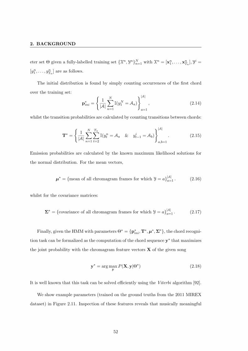
2. BACKGROUND
eter set Θ given a fully-labelled training set {Xn,Yn}Nn=1 with Xn = [xn1 , . . . ,x
nTn
],Yi =
[yn1 , . . . , ynTn
] are as follows.
The initial distribution is found by simply counting occurrences of the first chord
over the training set:
p∗ini =
{1
|A|
N∑n=1
I(yN1 = Aa)
}|A|a=1
, (2.14)
whilst the transition probabilities are calculated by counting transitions between chords:
T∗ =
{1
|A|
N∑n=1
Tn∑t=2
I(ynt = Aa & yit−1 = Ab)
}|A|a,b=1
. (2.15)
Emission probabilities are calculated by the known maximum likelihood solutions for
the normal distribution. For the mean vectors,
µ∗ = {mean of all chromagram frames for which Y = a}|A|a=1 . (2.16)
whilst for the covariance matrices:
Σ∗ = {covariance of all chromagram frames for which Y = a}|A|a=1 . (2.17)
Finally, given the HMM with parameters Θ∗ = {p∗ini,T∗,µ∗,Σ∗}, the chord recogni-
tion task can be formalized as the computation of the chord sequence y∗ that maximizes
the joint probability with the chromagram feature vectors X of the given song
y∗ = arg maxy
P (X,y|Θ∗) (2.18)
It is well known that this task can be solved efficiently using the Viterbi algorithm [92].
We show example parameters (trained on the ground truths from the 2011 MIREX
dataset) in Figure 2.11. Inspection of these features reveals that musically meaningful
52
2.8 Conclusion
parameters can be learned from the data, without need for expert knowledge. Notice,
for example, how the initial distribution is strongly peaked to starting on ‘no chord’, as
expected (most songs begin with no chord). Furthermore, we see strong self-transitions
in line with our expectation that chords are constant over several beats. Mean vectors
bear close resemblance to the pitches present within each chord and the covariance
matrix is almost diagonal, meaning there is little covariance between notes in chords.
2.8 Conclusion
In this chapter, we have discussed the foundations and definitions of chords, both in
the settings of musical theory and signal processing. We saw that there is no well-
defined notion of a musical chord, but that it is generally agreed to be a collection of
simultaneous notes or arpeggio. We also saw how chords can be used to define the key
of a piece, or vice-versa. Incorporating these two musical facets has been fruitful in the
task of automatic chord recognition.
Following this, we conducted a study of the literature concerning chord recogni-
tion from audio, concentrating on feature extraction, modelling, evaluation, and model
training/datasets. Upon investigating the annual benchmarking system MIREX, we
found that that the dominant architectures are chromagram features with HMM de-
coding, although more complex features and modelling strategies have also been em-
ployed. We also saw that, since the testing data are known to participants, the optimal
strategy is to overfit the test data as much as possible, meaning that these results may
be misleading as a definition of the state of the art.
53

2. BACKGROUND
Figure 2.11: HMM parameters, trained using Maximum likelihood on the MIREXdataset. Above, left: logarithm of initial distribution p∗
ini. Above, right: logarithmtransition probabilities T∗. Below, left: mean vectors for each chord µ∗. Below, right:covariance matrix Σ∗ for a C:maj chord. To preserve clarity, parallel minors for each chordand accidentals follow to the right and below.
54
3
Chromagram Extraction
This section details our feature extraction process. By far the most prevalent features
used in ACE are known as chromagrams (see chapter 2). Our features are strongly
related to these but are rooted in a sound theoretical foundation, based on the human
perception of loudness of sound.
This chapter is arranged as follows. Section 3.1 informs our approach to forming
loudness-based chromagrams. Sections 3.2 to 3.9 deal with the details of our feature
extraction process, and in section 3.10, we conduct experiments to show the predictive
power of these features using our baseline recognition method. We conclude in section
3.11.
3.1 Motivation
We seek to compute features that are useful in recognising chords, but firmly rooted
in a sound theoretical basis. The human auditory system is complex, involving the
inner, middle and outer ears, hair cells, and the brain. However, evidence exists that
shows that humans are more sensitive to changes frequency magnitude, rather than
temporal representations [24]. One way of doing this computationally is to take a
55
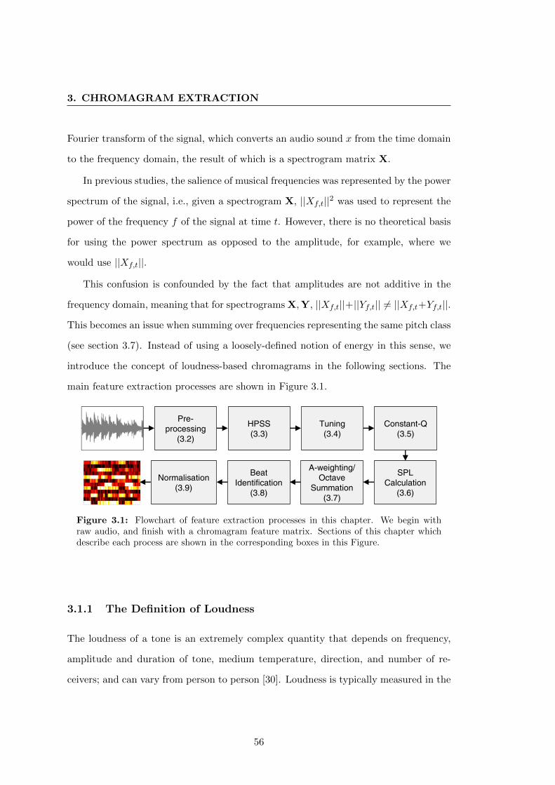
3. CHROMAGRAM EXTRACTION
Fourier transform of the signal, which converts an audio sound x from the time domain
to the frequency domain, the result of which is a spectrogram matrix X.
In previous studies, the salience of musical frequencies was represented by the power
spectrum of the signal, i.e., given a spectrogram X, ||Xf,t||2 was used to represent the
power of the frequency f of the signal at time t. However, there is no theoretical basis
for using the power spectrum as opposed to the amplitude, for example, where we
would use ||Xf,t||.
This confusion is confounded by the fact that amplitudes are not additive in the
frequency domain, meaning that for spectrograms X,Y, ||Xf,t||+||Yf,t|| 6= ||Xf,t+Yf,t||.
This becomes an issue when summing over frequencies representing the same pitch class
(see section 3.7). Instead of using a loosely-defined notion of energy in this sense, we
introduce the concept of loudness-based chromagrams in the following sections. The
main feature extraction processes are shown in Figure 3.1.
Pre-
processing
(3.2)
HPSS
(3.3)
Tuning
(3.4)
Constant-Q
(3.5)
Normalisation
(3.9)
Beat
Identification
(3.8)
A-weighting/
Octave
Summation
(3.7)
SPL
Calculation
(3.6)
Figure 3.1: Flowchart of feature extraction processes in this chapter. We begin withraw audio, and finish with a chromagram feature matrix. Sections of this chapter whichdescribe each process are shown in the corresponding boxes in this Figure.
3.1.1 The Definition of Loudness
The loudness of a tone is an extremely complex quantity that depends on frequency,
amplitude and duration of tone, medium temperature, direction, and number of re-
ceivers; and can vary from person to person [30]. Loudness is typically measured in the
56
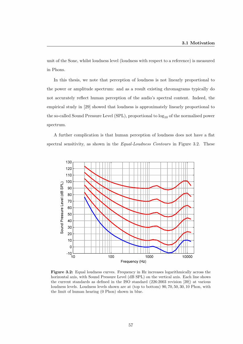
3.1 Motivation
unit of the Sone, whilst loudness level (loudness with respect to a reference) is measured
in Phons.
In this thesis, we note that perception of loudness is not linearly proportional to
the power or amplitude spectrum: and as a result existing chromagrams typically do
not accurately reflect human perception of the audio’s spectral content. Indeed, the
empirical study in [29] showed that loudness is approximately linearly proportional to
the so-called Sound Pressure Level (SPL), proportional to log10 of the normalised power
spectrum.
A further complication is that human perception of loudness does not have a flat
spectral sensitivity, as shown in the Equal-Loudness Contours in Figure 3.2. These
Figure 3.2: Equal loudness curves. Frequency in Hz increases logarithmically across thehorizontal axis, with Sound Pressure Level (dB SPL) on the vertical axis. Each line showsthe current standards as defined in the ISO standard (226:2003 revision [39]) at variousloudness levels. Loudness levels shown are at (top to bottom) 90, 70, 50, 30, 10 Phon, withthe limit of human hearing (0 Phon) shown in blue.
57
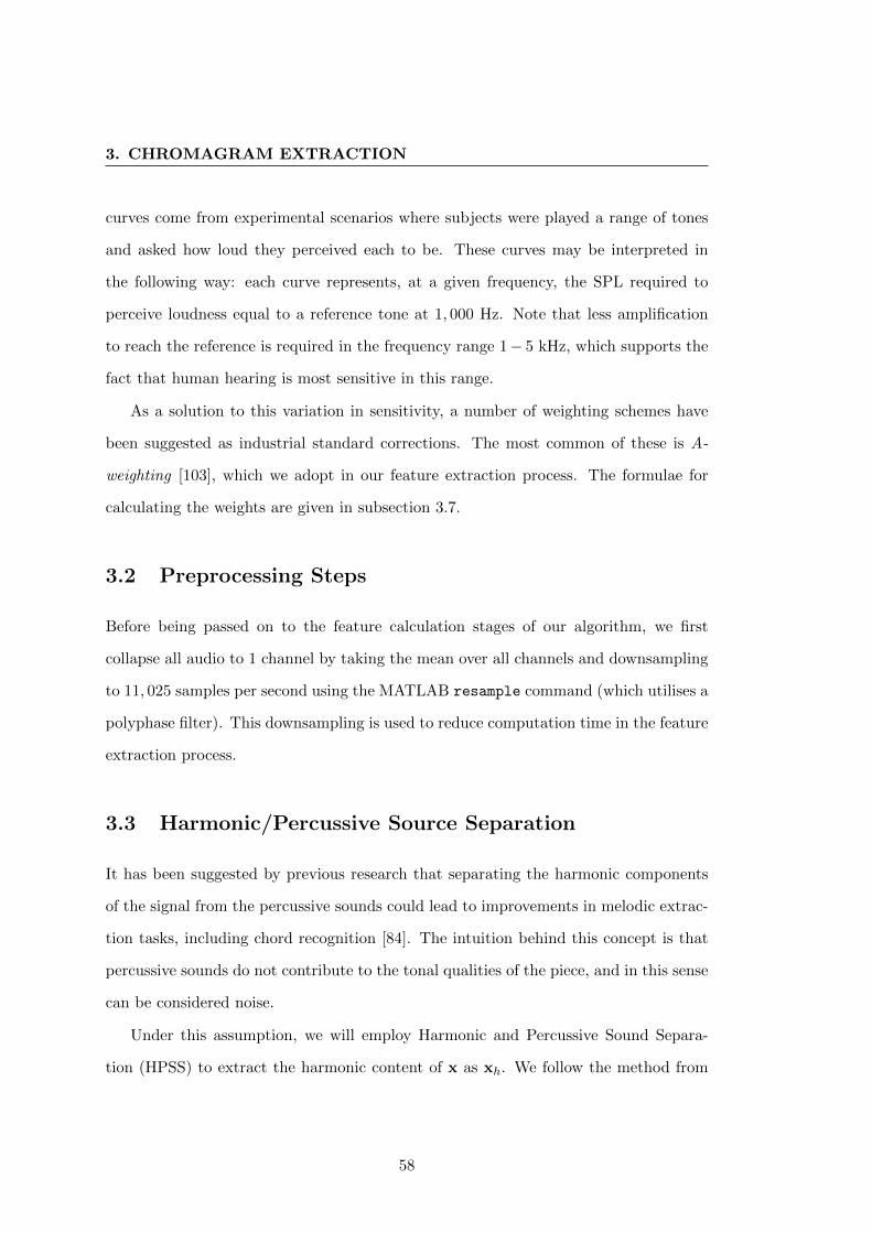
3. CHROMAGRAM EXTRACTION
curves come from experimental scenarios where subjects were played a range of tones
and asked how loud they perceived each to be. These curves may be interpreted in
the following way: each curve represents, at a given frequency, the SPL required to
perceive loudness equal to a reference tone at 1, 000 Hz. Note that less amplification
to reach the reference is required in the frequency range 1− 5 kHz, which supports the
fact that human hearing is most sensitive in this range.
As a solution to this variation in sensitivity, a number of weighting schemes have
been suggested as industrial standard corrections. The most common of these is A-
weighting [103], which we adopt in our feature extraction process. The formulae for
calculating the weights are given in subsection 3.7.
3.2 Preprocessing Steps
Before being passed on to the feature calculation stages of our algorithm, we first
collapse all audio to 1 channel by taking the mean over all channels and downsampling
to 11, 025 samples per second using the MATLAB resample command (which utilises a
polyphase filter). This downsampling is used to reduce computation time in the feature
extraction process.
3.3 Harmonic/Percussive Source Separation
It has been suggested by previous research that separating the harmonic components
of the signal from the percussive sounds could lead to improvements in melodic extrac-
tion tasks, including chord recognition [84]. The intuition behind this concept is that
percussive sounds do not contribute to the tonal qualities of the piece, and in this sense
can be considered noise.
Under this assumption, we will employ Harmonic and Percussive Sound Separa-
tion (HPSS) to extract the harmonic content of x as xh. We follow the method from
58

3.3 Harmonic/Percussive Source Separation
[84], where it is assumed that in a spectrogram, the harmonic component will have
low temporal variation but high spectral variation, with the converse true for per-
cussive components. Given a spectrogram W, the harmonic/percussive components
H = Ht,f ,P = Pt,f are found by minimizing
J(H,P) =1
2σ2H
∑t,f
(Ht,f−1 −Ht,f−1)2 +1
2σ2P
∑t,f
(Pt−1,f − Pt−1,f )2
subject to: Ht,f + Pt,f = Wt,f ,
Ht,f ≥ 0, Pt,f ≥ 0
The optimization scheme to solve this problem can be found in [84]. The HPSS algo-
rithm has a total of 5 parameters, which were set as suggested in [84]:
• STFT window length. Window length for computation of spectrogram - 1024
samples
• STFT hop length. Hop length for computation of spectrogram - 512 samples
• α Balance between horizontal and vertical components - 0.3
• γ Range compression parameter - 0.3
• kmax Number of iterations of the HPSS algorithm - 50
To illustrate the concept behind HPSS, we show a typical spectrogram decompo-
sition in Figure 3.3. Notice that the the harmonic component contains a more stable
horizontal component, whilst in the percussive component, more of the vertical com-
ponents remain. Audio inspection of the resulting waveforms confirmed that the HPSS
technique had in fact captured much of the harmonic component in one waveform,
whilst removing the percussion.
59
3. CHROMAGRAM EXTRACTION
(a)
Enti
resp
ectr
um
(b)
Harm
onic
com
ponen
tsof
signal
(c)
Per
cuss
ive
com
ponen
tsof
signal
Fig
ure
3.3
:Il
lust
rati
onof
Har
mon
icP
ercu
ssiv
eS
ou
rce
Sep
ara
tion
alg
ori
thm
.T
hre
esp
ectr
aare
show
n.
InF
igu
re3.3
a,
we
show
the
spec
trog
ram
ofa
30se
con
dse
gmen
tof
‘Hey
Ju
de’
(Len
non
-McC
art
ney
).F
igu
res
3.3
ban
d3.3
csh
owth
ere
sult
ing
harm
onic
an
dp
ercu
ssiv
esp
ectr
ogra
ms
afte
rp
erfo
rmin
gH
PS
S,
resp
ecti
vely
.
60
3.4 Tuning Considerations
After computing the spectra of the harmonic and percussive elements, we can invert
the transforms to obtain the decomposition x = xh + xp. Discarding the percussive
component of the audio, we now work solely with the harmonic component.
3.4 Tuning Considerations
Before computing our Loudness Based Chromagrams, we must consider the possibility
that the target waveform is not tuned in standard pitch. Most modern recordings are
tuned with A4 = 440 Hz under the twelve-tone equal tempered scale [14]. Deviating
from this assumption could lead to note frequencies estimated incorrectly, meaning that
the chromagram bins are incorrectly estimated which could degrade performance.
Our tuning method follows that of [26], where an initial histogram is calculated of
all frequencies found, relative to standard pitch. The “correct” tuning is then found by
taking the bin with the largest number of entries. The centre frequencies of the spec-
trum can then be augmented according to this information. We provide an illustrative
example of the tuning algorithm in Figure 3.4.
3.5 Constant Q Calculation
Having pre-processed our waveform, we are ready to compute a spectral representation.
The most natural choice of transform to the frequency domain may be the Fourier
transform [9]. However, this transform has a fixed window size, meaning that if too
small a window is used, some low frequencies may be missed (as they will have a period
larger than the window). Conversely, if the window size used is too large, a poor time
resolution will be obtained.
A balance between time and frequency resolution can be found by having frequency-
dependent window sizes, a concept that can be implemented via a Constant-Q spec-
trum. The Q here relates to the ratio of successive window sizes, as explained in the
61
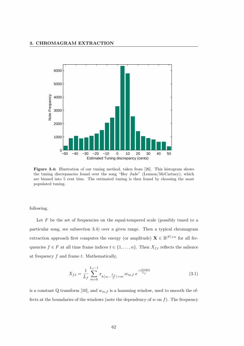
3. CHROMAGRAM EXTRACTION
−50 −40 −30 −20 −10 0 10 20 30 40 500
1000
2000
3000
4000
5000
6000
Estimated Tuning discrepancy (cents)
Not
e F
requ
ency
Figure 3.4: Illustration of our tuning method, taken from [26]. This histogram showsthe tuning discrepancies found over the song “Hey Jude” (Lennon/McCartney), whichare binned into 5 cent bins. The estimated tuning is then found by choosing the mostpopulated tuning.
following.
Let F be the set of frequencies on the equal-tempered scale (possibly tuned to a
particular song, see subsection 3.4) over a given range. Then a typical chromagram
extraction approach first computes the energy (or amplitude) X ∈ R|F |×n for all fre-
quencies f ∈ F at all time frame indices t ∈ {1, . . . , n}. Then Xf,t reflects the salience
at frequency f and frame t. Mathematically,
Xf,t =1
Lf
Lf−1∑m=0
xhdst−
Lf2e+m
.wm,f .e−j2πQm
Lf (3.1)
is a constant Q transform [10], and wm,f is a hamming window, used to smooth the ef-
fects at the boundaries of the windows (note the dependency of w on f). The frequency
62
3.6 Sound Pressure Level Calculation
dependent bandwidth Lf is defined as Lf = Q srf , where Q represents the constant res-
olution factor, and sr is the sampling rate of xh. d·e represents the ceiling function,
and j is the imaginary unit.
We note here that we do not use a “hop length” of the windows used in our constant-
Q spectrum. Instead, we centre the windows on every sample from the signal. In
addition to this, we found that by choosing larger windows than are specified by the
constant-Q ratios, performance increased. This was realised by multiplying all window
lengths by a constant factor to pick up more energy, which we call a “Power factor”,
optimised on the full beat-synchronised loudness-based chromagram. Note that this is
equivalent to using a larger value of Q and then decimating in frequency. We found
that a power factor of 5 worked well for treble frequencies, whilst 3 was slightly better
for bass frequencies, although results were not particularly sensitive to this parameter.
3.6 Sound Pressure Level Calculation
This section deals with our novel loudness calculation for chromagram feature extrac-
tion. As described in subsection 3.1.1, the key concept is to transform the spectrum in
such a way that it more closely relates to the human auditory perception of the loud-
ness of the frequency powers. This is achieved by first computing the sound pressure
level of the spectrum, and then correcting for the fact that the powers of low and high
frequencies require higher sound pressure levels for the same perceived loudness as do
mid-frequencies [29].
Given the constant-Q spectrogram representation X, we compute the Sound Pres-
sure Level (SPL) representation by taking the logarithm of the energy spectrum. A
reference pressure level pref is needed, but as we shall see in subsection 3.9, specifying
a specific value is in fact not required and so in practice can be set to 1. We compute
63
3. CHROMAGRAM EXTRACTION
the loudness of the spectrum therefore via:
SPLf,t = 10 log10
(‖Xf,t‖2
‖pref ‖2
), f ∈ F, t = 1, . . . , n, (3.2)
where pref indicates a reference pressure level. A small constant may be added to
‖Xf,t‖2 to avoid numerical problems in this calculation, although we did not experience
this issue in any of our data.
3.7 A-Weighting & Octave Summation
To compensate for the varying loudness sensitivity across the frequency range, we use
A-weighting [103] to transform the SPL matrix into a representation of the perceived
loudness of each of the frequencies:
Lf,t = SPLf,t +A(f), f ∈ F, t = 1, . . . , n, (3.3)
where the A-weighting functions are as quoted from [103]:
RA(f) = 122002·f4
(f2+20.62)·√
(f2+107.72)(f2+737.92)·(f2+122002),
A(f) = 2.0 + 20 log10(RA(f)).
(3.4)
We are left with a sound pressure level matrix that relates to the human perception
of the loudness of frequency powers in a musical piece. Taking advantage of octave
equivalence, we now sum over frequencies which belong to the same pitch class. It is
known that loudnesses are additive if they are not close in frequency [97]. This allows
us to sum up loudness of sounds in the same pitch class, yielding an octave-summed
loudness matrix, LO:
LOp,t =
∑f∈F
δ(M(f) + 1, p)Lf,t, p = 1, . . . , 12, t = 1, . . . , n. (3.5)
64
3.8 Beat Identification
Here δ denotes an indicator function and
M(f) =
(⌊12 log2
(f
fA
)+ 0.5
⌋+ 69
)mod 12. (3.6)
Exploiting the fact the chords rarely change between beats [35], we next beat synchro-
nise our chromagram features.
3.8 Beat Identification
We use an existing technique to estimate beats in the audio [26], and therefore extract
a vector of estimated beat times b = (b1, b2, . . . , bT−1). To this we add artificial beats
at time 0, and the end of the song, and take the median chromagram vector between
subsequent beats to beat-synchronise our chromagrams. This yields an octave-summed,
beat synchronised feature composed of T frames:
LOBf,t = {median of LO between beats bt−1 and bt} for f = 1, . . . 12, t = 2, . . . , T.
3.9 Normalisation Scheme
Finally, to account for the fact that overall sound level should be irrelevant in estimating
harmonic content, our loudness-based chromagram C ∈ R12×T is obtained by range-
normalizing LOB:
Cp,t =
LOBp,t −min
p′LOBp′,t
maxp′
LOBp′,t −min
p′LOBp′,t
, ∀p, t. (3.7)
Note that this normalization is invariant with respect to the reference level, and a
specific pref is therefore not required and can be set to 1 in practice. Note also that
the A-weighting scheme used is a non-linear addition, such that its effect is not lost in
the normalisation.
65
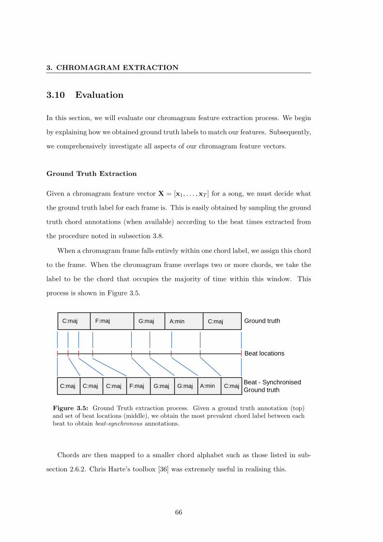
3. CHROMAGRAM EXTRACTION
3.10 Evaluation
In this section, we will evaluate our chromagram feature extraction process. We begin
by explaining how we obtained ground truth labels to match our features. Subsequently,
we comprehensively investigate all aspects of our chromagram feature vectors.
Ground Truth Extraction
Given a chromagram feature vector X = [x1, . . . ,xT ] for a song, we must decide what
the ground truth label for each frame is. This is easily obtained by sampling the ground
truth chord annotations (when available) according to the beat times extracted from
the procedure noted in subsection 3.8.
When a chromagram frame falls entirely within one chord label, we assign this chord
to the frame. When the chromagram frame overlaps two or more chords, we take the
label to be the chord that occupies the majority of time within this window. This
process is shown in Figure 3.5.
Beat - Synchronised
Ground truth
Ground truth C:maj F:maj G:maj A:min C:maj
C:maj C:maj C:maj F:maj G:maj G:maj A:min C:maj
Beat locations
Figure 3.5: Ground Truth extraction process. Given a ground truth annotation (top)and set of beat locations (middle), we obtain the most prevalent chord label between eachbeat to obtain beat-synchronous annotations.
Chords are then mapped to a smaller chord alphabet such as those listed in sub-
section 2.6.2. Chris Harte’s toolbox [36] was extremely useful in realising this.
66
3.10 Evaluation
Evaluation
To evaluate the effectiveness of our chromagram representation, we collected audio
and ground truth annotations for the MIREX dataset (179 songs by The Beatles1, 19
by Queen, 18 Zweieck). Wishing to see the effect that each stage of processing had
on recognition accuracy, we incrementally increased the number of signal processing
techniques. We refer to the loudness-based chromagram described in Sections 3.2 to
3.9 as the Loudness Based Chromagram, or LBC. In summary the features used were:
• Constant-Q - a basic constant-Q transform of the signal, taken over frequencies
A1 (55 Hz) to G]6 (∼ 1661 Hz)
• Constant-Q + HPSS - as above, but computed on the harmonic component of
the audio, calculated using the Harmonic Percussive Sound Separation detailed
in subsection 3.3.
• Constant-Q + HPSS + Tuning - as above, with frequency bins tuned to the
nearest semitone by the algorithm in subsection 3.4.
• no A-weighting - as above, with the loudness of the spectrum calculated as the
log10 of the spectrum (without A-weighting).
• LBC - as above, with the loudnesses weighted according to human loudness sen-
sitivity.
• Beat-synchronised LBC - as above, where the median loudnesses across each pitch
are taken between beats identified by the algorithm described in 3.8.
All feature vectors were range-normalised after computation. We show the chroma-
grams for a particular song for visual comparison in Figure 3.6. Performance in this song
increased from 37.37% to 84.02% by use of HPSS, tuning, loudness and A-weighting
(the ground truth chord label for the entirety of this section is A:maj).
1“Revolution 9” (Lennon/McCartney) was removed as it was deemed to have no harmonic content
67

3. CHROMAGRAM EXTRACTION
In the first subplot we see that by working with the harmonic component of the
audio, we are able to pick up the C] note in the first beat, and lose some of the noise
in pitch classes A to B. Moving on, we see that the energy from the dominant pitch
classes (A and E) are incorrectly mapped to the neighbouring pitch classes, which is
corrected by tuning (estimated tuning for this song was -40 cents). Calculating the
loudness of this chromagram enhances the loudness of the pitches A and E, which is
further enhanced by A-weighting. Finally, beat-synchronisation means that each frame
now corresponds to a musically meaningful time scale. Ground truths were sampled
according to each feature set and reduced to major and minor chords only, with an
additional “no chord” symbol.
An HMM as per Section 2.7 was used to identify chords in this experiment, trained
and tested on the MIREX dataset. Chord similarity per song was simply measured by
number of correctly identified frames divided by total number of frames and we used
either ARCO or TRCO (see subsection 2.6.1) as the overall evaluation scheme. Overall
performances are shown in Table 3.1. We also conducted the Wilcoxon rank sum test
to test the significance of improvements seen.
Table 3.1: Performance tests for different chromagram feature vectors, evaluated usingAverage Relative Correct Overlap (ARCO) and Total Relative Correct Overlap (TRCO).p−values for the Wilcoxon rank sum test on successive features are also shown.
Performance (%)
Chromagram Type ARCO TRCO Significance
Constant-Q 59.40 59.08 -Constant-Q with HPSS 58.27 57.95 0.40Constant-Q with HPSS and Tuning 61.55 61.17 0.01LBC (no A-weighting) 79.92 80.02 2.95e− 43LBC 80.19 80.27 0.78Beat-synchronised LBC 80.97 80.91 0.34
Investigating the performances in Table 3.1, we see large improvements when using
advanced signal processing techniques, from 59.08% to 80.91% Total Relative Correct
68
3.10 Evaluation
Overlap. Investigating each component separately, we see that Harmonic Percussive
Sound Separation decreases the performance slightly over the full waveform. This
decrease is small in magnitude and can be explained by the suboptimal selection of
the power factor in the chromagram extraction1. Tuning of musical frequencies shows
an improvement of about 3% over untuned frequency bins, confirming that the tuning
method we used correctly identifies and adjusts songs that are not tuned to standard
pitch.
By far the largest improvement can be seen by taking the log of the spectrum
(LBC, row 4), with a very slight improvement upon adding A-weighting. Although this
increase is not significant, we include it in the feature extraction to ensure the loudness
we calculate models the human perception of loudness. Finally, beat-synchronising
both features and annotations offers an improvement of slightly less than 1% absolute
improvement, and has the additional benefit of ensuring that chord changes occur
on (predicted) beats. Investigating the significance of our findings, we see that the
introduction of tuning and loudness calculation offer significant improvements at the
5% level (p < 0.05).
The results presented here are comparable to the pretrained or expert systems in
MIREX evaluations in section 2.6.4. A thorough investigation of train/test scenarios
is required to test if our model is comparable to train/test algorithms, although this is
postponed until future chapters.
1Recall that this parameter was optimised on the fully beat-synchronised chromagram, A fixedpower factor of 5 was used throughout these experiments, which was found to perform optimallyover these experimental conditions. Although applying HPSS to the spectrogram degraded perfor-mance slightly, the change is small in magnitude (around 1-1.5% absolute) and is consistent with theperceptually-motived model of harmony presented within this thesis, and is therefore included in allfuture experiments
69
3. CHROMAGRAM EXTRACTION
3.11 Conclusions
In this chapter, we introduced our motivation for calculating loudness based chroma-
grams for the task of audio chord estimation. We saw how the notion of perception
of loudness was difficult to define, although under some relaxed assumptions we can
model it closely. One of the key findings of these studies was that the human auditory
response to the loudness of pitches was non-linear with respect to frequency. With
these studies in mind, we computed loudness based chromagrams that are rigorously
defined and follow the industrial standard of A-weighting of frequencies.
These techniques were enhanced by injecting some musical knowledge into the fea-
ture extraction. For example, we tuned the frequencies to correspond to the musical
scale, removed the percussive element of the audio, and beat-synchronised our features.
Experimentally, we saw that by introducing these techniques we achieve a performance
of 80.97% TRCO on a set of 217 songs.
70
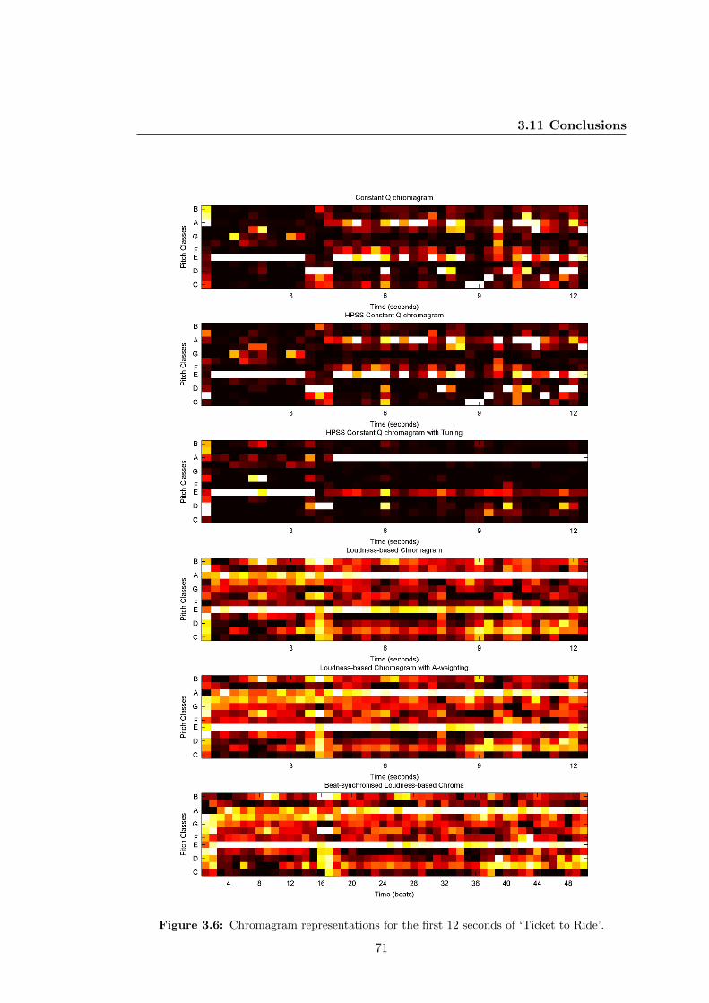
3.11 Conclusions
Figure 3.6: Chromagram representations for the first 12 seconds of ‘Ticket to Ride’.
71
3. CHROMAGRAM EXTRACTION
72

4
Dynamic Bayesian Network
In this chapter, we describe our model for the recognition of chords, keys and bass
notes from audio. Having described our feature extraction process in chapter 3, we
must decide on how to assign a chord, key and bass label to each frame.
Motivated by previous work in Dynamic Bayesian Networks (DBNs, [65? ]), our
approach to the automatic recognition of chords from audio will involve the construction
of a graphical model with hidden nodes representing the musical features we wish to
discover, and observed nodes representing the audio signal.
As shown in subsection 2.4.4, DBNs have been shown to be successful in reconstruct-
ing chord sequences from audio when trained using expert knowledge [62]. However,
it is possible that these models overfit the available data by hand-tuning of parame-
ters. We will counter this by employing machine learning techniques to infer parameter
settings from fully-labelled data, and testing our results using cross-validation.
The remainder of this chapter is arranged as follows: section 4.1 outlines the mathe-
matical framework for our model. In section 4.2, we build up the DBN, beginning with
a simple HMM and adding nodes, incrementally increasing the model complexity. All
of this work will be based on the minmaj alphabet of 12 major chords, 12 minor chords
and a “No Chord” symbol; and we also discuss issues of computational complexity in
73
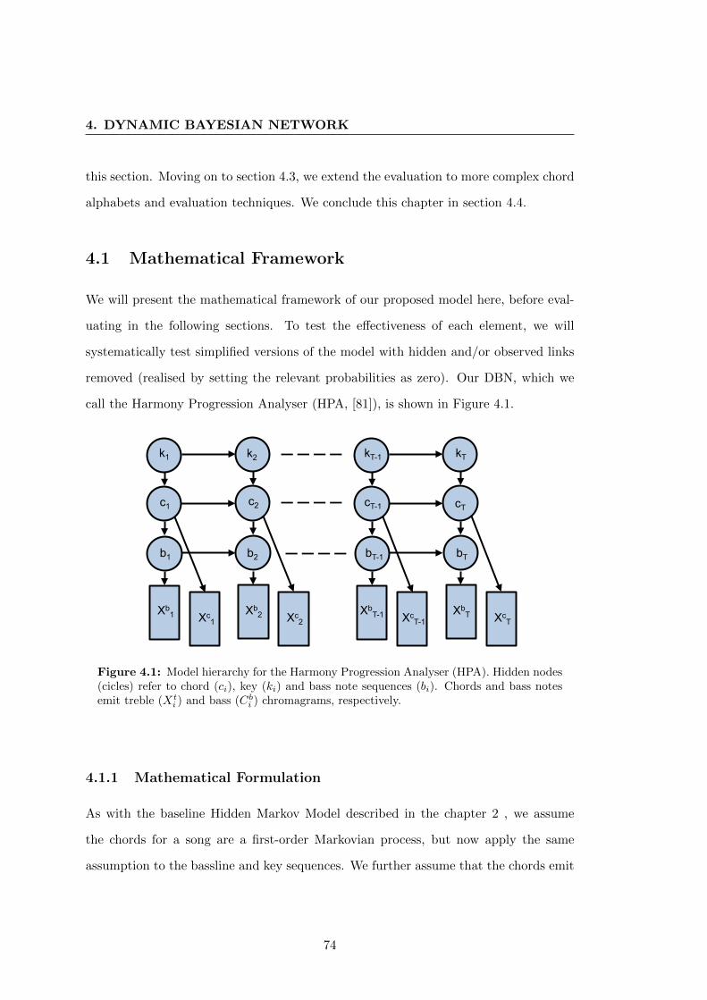
4. DYNAMIC BAYESIAN NETWORK
this section. Moving on to section 4.3, we extend the evaluation to more complex chord
alphabets and evaluation techniques. We conclude this chapter in section 4.4.
4.1 Mathematical Framework
We will present the mathematical framework of our proposed model here, before eval-
uating in the following sections. To test the effectiveness of each element, we will
systematically test simplified versions of the model with hidden and/or observed links
removed (realised by setting the relevant probabilities as zero). Our DBN, which we
call the Harmony Progression Analyser (HPA, [81]), is shown in Figure 4.1.
cT-1
XbT-1 Xc
T-1
bT-1
kT-1
XbT Xc
T
cT
bT
kT
c1
Xb1 Xc
1
b1
k1
Xb2 Xc
2
c2
b2
k2
Figure 4.1: Model hierarchy for the Harmony Progression Analyser (HPA). Hidden nodes(cicles) refer to chord (ci), key (ki) and bass note sequences (bi). Chords and bass notesemit treble (Xt
i ) and bass (Cbi ) chromagrams, respectively.
4.1.1 Mathematical Formulation
As with the baseline Hidden Markov Model described in the chapter 2 , we assume
the chords for a song are a first-order Markovian process, but now apply the same
assumption to the bassline and key sequences. We further assume that the chords emit
74
4.1 Mathematical Framework
a treble chromagram, whilst the bass notes emit a bass chromagram. This is shown
by the fact that HPA’s adopted topology consists of three hidden and two observed
variables. The hidden variables correspond to the key K, the chord label C and the
bass B annotations.
Under this representation, a chord is decomposed into two aspects: chord label and
bass note. Taking the chord G:maj/b7 as an example, the chord state is c = G:maj and
the bass state is b = F. Accordingly, we compute two chromagrams for two frequency
ranges: the treble chromagram Xc, which is emitted by the chord sequence c and the
bass chromagram Xb, which is emitted by the bass sequence b. The reason of applying
this decomposition is that different chords can share the same bass note, resulting in
similar chroma features in the low frequency domain. We hope that by using separated
variables we can increase variation between chord states, so as to better recognise in
particular complex chords. Note that this definition of bass note is non-standard: we
are not referring to the note which the bass instrument (i.e. bass guitar, left hand
piano) is playing, but instead the pitch class of the current chord which has lowest
pitch in the chord.
HPA has a similar structure to the chord estimation model defined by Mauch [62].
Note however the lack of metric position (we are aware of no data to train this node),
and that that the conditional probabilities in the model are different. HPA has, for
example, no link from chord t− 1 to bass t, but instead has a link from bass pitch class
t− 1 to bass pitch class t.
Under this framework, the set Θ of HPA has the following parameters:
Θ ={pi(k1), pi(c1), pi(b1), ptr(kt|kt−1), ptr(ct|ct−1, kt), ptr(bt|ct), ptr(bt|bt−1),
pe(Xct |ct), pe(Xb
t |bt)}, (4.1)
where pi, ptr and pe denote the initial, transition and emission probabilities, respec-
75
4. DYNAMIC BAYESIAN NETWORK
tively. The joint probability of the chromagram feature vectors {Xc, Xb} and the
corresponding annotation sequences {k, c,b} of a song is then given by the formula1
P (Xc,Xb,k, c,b|Θ) = pi(k1)pi(c1)pi(b1)
T∏t=2
pt(kt|kt−1)ptr(ct|ct−1, kt)ptr(bt|ct)×
pt(bt|bt−1)
T∏t=1
pe(Xct |ct)pe(Xb
t |bt). (4.2)
4.1.2 Training the Model
For estimating the parameters in Equation 4.1, we use Maximum Likelihood Estima-
tion, analogous to the HMM setting in section 2.7. Bass notes were extracted directly
from the chord labels, whilst for keys we used the corresponding key set from the
MIREX dataset2 (although this data is not available to participants of the MIREX
evaluations).
The amount of key data in these files is sparse when compared to chords. Consider-
ing only major and minor keys3 as well as a ‘No Key’ symbol, we discovered that almost
all keys appeared at least once (22/25 keys, 88%), although most key transitions were
not seen. Of the 252 = 625 possible key transitions we saw just 130, severely limiting
the amount of data we have for key transitions. To counteract this, following Ellis et.
al [26] in all models involving key information we first transposed each frame to an
arbitrary “home key” (we chose C:maj and A:min) and then learnt parameters in these
two canonical major/minor keys. Model parameters were then transposed 12 times,
leaving us with approximately 12 times as much training data for the hidden chain.
Key to chord transitions were also learnt in this way.
Bass note transitions and initial distribution were learnt using the same maximum
1Note that we use the approximation ptr(bt|bt−1, ct) ∼ ptr(bt|ct)ptr(bt|bt−1), which from a purelyprobabilistic perspective is not correct. However, this simplification reduces computational and statis-tical cost and results in better performance in practice.
2publicly available at http://www.isophonics.net/3Modal keys such as “Within You Without You”, (Harrison, in a C] modal key) were assigned to
a related major or minor key to our best judgement
76
4.1 Mathematical Framework
likelihood estimation as described in chapter 2. Similarly, bass note emissions were
assumed to come from a 12–dimensional Gaussian distribution, which was learned from
chromagram/bass note pairs using maximum likelihood estimation.
4.1.3 Complexity Considerations
Given the large number of nodes in our graphical model, we must consider the compu-
tational practicalities of decoding the optimal chord, key and bass sequences from the
model. Given a chord, key and bass alphabet size of sizes |Ac|, |Ak|, |Ac|, respectively,
the time complexity for Viterbi decoding a song with T frames is O(|Ac|2|Ak|2|Ac|2|T |),
which easily becomes prohibitive as the alphabets become of reasonable size. To coun-
teract this, we employ a number of search space reduction techniques, detailed below.
Chord Alphabet Constraint
It is unlikely that any one song will use all the chords available in the alphabet in a
song. Therefore, we can reduce the number of chord nodes to search if a chord alphabet
is known, before decoding. To achieve this, we ran a simple HMM with max-gamma
decoder [92] over the observation probability matrix for a song (using the full frequency
range), and obtained such an alphabet, A′c. Using this, we are able to set the transition
probabilities for all chords not in this set to be zero, thus drastically reducing our search
space:
p′(ct|ct−1, k) =
p(ct|ct−1, k) if ct, ct−1 ∈ A
′c
0 otherwise
(4.3)
Key Transition Constraint
Musical theory tells us that not all key transitions are equally likely, and that if a key
modulates it will most likely to be a related key [51]. Thus, we propose to rule out key
changes that are rarely seen in the training phase of our algorithm, a process known
77
4. DYNAMIC BAYESIAN NETWORK
as threshold pruning in dynamic programming [8]. Thus, we may devise new transition
probabilities as:
p′(k|k) =
p(k|k) if |kt = k, kt−1 = k| > γ
0 otherwise
(4.4)
where γ ∈ {Z+ ∪ 0} is a threshold parameter that must be specified in advance.
Chord to Bass Constraint
Similarly, we expect that a given chord will be unlikely to emit all possible bass notes.
We may therefore apply another threshold τ to constrain the number of emissions we
consider here. Thus we may set:
p′(b|c) =
p(b|c) if |ct = c, bt = b| > τ.
0 otherwise
(4.5)
In our previous work [81], we discovered that by setting γ = 10, τ = 3 we obtain an
approximate 10-fold reduction in decoding time, whilst losing just 0.1% in performance.
We will therefore employ these parameters throughout the remainder of this thesis.
p′(ct|ct−1, k), p′(k|k) and p′(b|c) were subsequently normalised to sum to 1 to ensure
they met the probability criterion.
4.2 Evaluation
This section deals with our experimental validation of our model. We will begin with
a baseline HMM approach to chord recognition, which can be realised as using HPA
with all key and bass nodes disabled. To ensure that all frequencies were covered, we
ran this model using a chromagram that covered the entire frequency range (A1-G]6).
Next, we studied the effectiveness of a Key-HMM, which had additional nodes
78

4.2 Evaluation
for key to chord transitions and key self-transitions. Penultimately, we allowed the
model to detect bass notes, and split the chromagram into a bass (A1-G]3) and treble
(A4-G]6) range, before investigating the full HPA architecture. Note that the bass and
treble chromagrams are split arbitrarily into two three octave representations. Different
bass/treble definitions may lead to improved performance but are not considered in this
thesis.
4.2.1 Experimental Setup
We will first investigate the effectiveness of a simple HMM on the MIREX dataset under
a train/test scenario. Under this setting, each fully-labelled training song is designated
to be either a training song on which to learn parameters, or a test song for evaluation.
To achieve balanced splits, we took approximately 1/3 of each album into the test
set, with the remainder as training, and performed 3-fold cross-validation, ensuring that
our results were comparable to the MIREX evaluations. This procedure was repeated
100 times, and performance was measured on the frame level using either TRCO or
ARCO as the average over the three folds. As previously mentioned, to investigate the
effect that various hidden and observed nodes had on performance, we disabled several
of the nodes, beginning at first with a simple HMM as per chapter 3. In summary, the
4 architectures investigated are:
• HMM. A Hidden Markov Model with hidden nodes representing chords and an
emission chromagram ranging from A1 to G]6.
• Key-HMM. As above, with an additional hidden key chain and key to chord links.
• Key-Bass-HMM. As above, with distinct chroma for the bass (A1-G]3) and treble
(A4-G]6) frequencies, and an accompanying chord to bass node.
• HPA. Full Harmony Progression Analyser, i.e. the above with additional bass-to-
bass links.
79

4. DYNAMIC BAYESIAN NETWORK
We begin by discussing the chord accuracies of the above models.
4.2.2 Chord Accuracies
Chord accuracies for each model are shown in Table 4.1. As can be seen directly from
Table 4.1: Chord recognition performances using various crippled versions of HPA. Per-formance is measured using Total Relative Correct Overlap (TRCO) or Average RelativeCorrect Overlap (ARCO), and averaged over 100 repetitions of a 3-fold cross-validationexperiment. Variances across these repetitions are shown after each result, and the bestresults are shown in bold.
TRCO (%) ARCO (%)
Train Test Train Test
HMM 81.25± 0.28 78.40± 0.64 81.22± 0.32 78.93± 0.66Key-HMM 79.10± 0.28 80.43± 0.56 79.26± 0.30 80.67± 0.60Key-Bass HMM 82.34± 0.26 80.26± 0.58 82.60± 0.27 81.03± 0.59HPA 83.52± 0.28 81.56± 0.58 83.64± 0.30 82.22± 0.63
Table 4.1, HPA attains the best performance under both evaluation schemes in both
training and testing phases. In general, we expect the training performance of the
model to increase as the complexity of the model increases down the rows, although
the HMM appears to buck this trend, offering superior performance to the Key-HMM
(rows 1 and 2). However, this pattern is not repeated in the test scenario, suggesting
that the HMM is overfitting the training data in these instances.
The fact that performance increases as the model grows in intricacy demonstrates
the power of the model, and also confirms that we have enough data to train it efficiently.
This result is encouraging, as it shows that it is possible to learn chord models from
fully-labelled data, and also gives us hope that we might build a flexible model capable
of performing chord estimation different artists and genres. The generalisation potential
of HPA will be investigated in chapter 5.
80
4.2 Evaluation
Statistical Significance
We now turn our attention to the significance of our findings. Over a given number
of cross-validations (in our case, 100), we wish to see if the improvements we have
found are genuine enhancements or could be due to random fluctuations in the data.
Upon inspecting the results in Table 4.1, performances were normally distributed across
repetitions of the 3-fold cross-validations.
Therefore, 1-sided, paired t-tests were conducted to assess if each stage of the al-
gorithm was improving on the previous one. With the sole exception of HMM vs.
Key-HMM in training, all models exhibited statistically significant improvements, as
evidenced by p-values of less than 10−25 in both train and test experiments.
4.2.3 Key Accuracies
Each experimental setup except the HMM also outputs a predicted key sequence for
the song. We measured key accuracy in a frame-wise manner, but noticed that the
percentage of frames where the key was correctly identified was strongly non-Gaussian,
as we were generally either predicting the correct key for all frames or the incorrect
key. Providing a mean of such a result is misleading, so we chose instead to provide
the histograms which show the average performance over the 100 repetitions of 3-fold
cross-validation, shown in Figure 4.2.
The performance here is not as high as we may expect, given the accuracy attained
on chord estimation. Reasons for this may include that the key nodes (see Figure
4.1) have no input from other nodes and that evaluation is measured inappropriately
as correct or incorrect, whereas a more flexible metric allowing for related keys to be
considered may be more appropriate. Investigating these scenarios is part of our future
work.
81
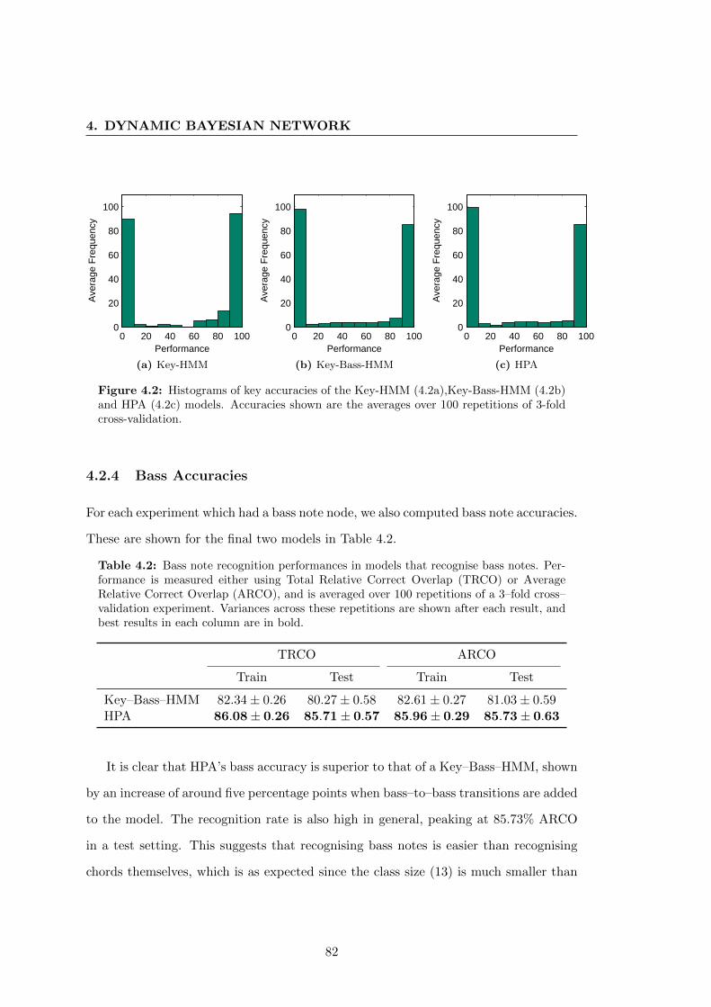
4. DYNAMIC BAYESIAN NETWORK
0 20 40 60 80 1000
20
40
60
80
100
Performance
Ave
rage
Fre
quen
cy
(a) Key-HMM
0 20 40 60 80 1000
20
40
60
80
100
Performance
Ave
rage
Fre
quen
cy
(b) Key-Bass-HMM
0 20 40 60 80 1000
20
40
60
80
100
Performance
Ave
rage
Fre
quen
cy
(c) HPA
Figure 4.2: Histograms of key accuracies of the Key-HMM (4.2a),Key-Bass-HMM (4.2b)and HPA (4.2c) models. Accuracies shown are the averages over 100 repetitions of 3-foldcross-validation.
4.2.4 Bass Accuracies
For each experiment which had a bass note node, we also computed bass note accuracies.
These are shown for the final two models in Table 4.2.
Table 4.2: Bass note recognition performances in models that recognise bass notes. Per-formance is measured either using Total Relative Correct Overlap (TRCO) or AverageRelative Correct Overlap (ARCO), and is averaged over 100 repetitions of a 3–fold cross–validation experiment. Variances across these repetitions are shown after each result, andbest results in each column are in bold.
TRCO ARCO
Train Test Train Test
Key–Bass–HMM 82.34± 0.26 80.27± 0.58 82.61± 0.27 81.03± 0.59HPA 86.08± 0.26 85.71± 0.57 85.96± 0.29 85.73± 0.63
It is clear that HPA’s bass accuracy is superior to that of a Key–Bass–HMM, shown
by an increase of around five percentage points when bass–to–bass transitions are added
to the model. The recognition rate is also high in general, peaking at 85.73% ARCO
in a test setting. This suggests that recognising bass notes is easier than recognising
chords themselves, which is as expected since the class size (13) is much smaller than
82

4.3 Complex Chords and Evaluation Strategies
in the chord recognition case (25). Paired t–tests were conducted as per subsection
4.2.2 to compare the Key–Bass HMM and HPA, and we observed p–values of less than
10−100 in all cases.
What remains to be seen is how bass note recognition affects chord inversion accu-
racy, although this has been noted by previous authors [65]. We will investigate this
hypothesis in HPA’s context in the following section.
4.3 Complex Chords and Evaluation Strategies
4.3.1 Increasing the chord alphabet
So far, all of our experiments have been conducted on an alphabet of major and minor
chords only. However, as mentioned in chapter 2, there are many other chord types
available to us. We therefore defined 4 sets of chord alphabets for advanced testing,
which are listed in Table 4.3.
Table 4.3: Chord alphabets used for evaluation purposes. Abbreviations: MM = MatthiasMauch, maj = major, min = minor, N = no chord, aug = augmented, dim = diminished,sus2 = suspended 2nd, sus4 = suspended 4th, maj6 = major 6th, maj7 = major 7th, 7 =(dominant 7), min7 = minor 7th, minmaj7 = minor, major 7th, hdim7 = half-diminished7 (diminished triad, minor 7th).
Alphabet A |A| Chord classes
Minmaj 25 maj,min,N
Triads 73 maj,min,aug,dim,sus2,sus4,N
MM 97 maj,min,aug,dim,maj6,maj7,7,min7,X,N
Quads 133 maj,min,aug,dim,sus2,sus4,maj7,min7,7,minmaj7,hdim7,N
Briefly, Triads is a set of major and minor thirds with optional diminished/perfect/augmented
fifths, as well as two “suspended” chords (sus2 = (1,2,5), sus4 = (1,4,5)). MM is
an adaptation of Matthias Mauch’s alphabet of 121 chords [62], although we do not
consider chord inversions such as maj/3, as we consider this to be an issue of evaluation.
Chords labelled as X are not easily mapped to one of the classes listed in [62], and are
83

4. DYNAMIC BAYESIAN NETWORK
always considered incorrect (examples include A:(1) and A:6). Quads is an extension
of Triads, with some common 4-note 7th chords.
We did not attempt to recognise any chords containing intervals above the octave,
since in a chromagram representation we can not distinguish between, for example,
C:add9 and Csus2. Also note that we do not consider inversions of chords such as
C:maj/3 to be unique chord types, although we will consider these chords in evaluation
(see 4.3.2). Reading the ground truth chord annotations and simplifying into one of
the alphabets in Table 4.3 was done via a simple hand-made map.
Larger chord alphabets such as MM pose an interesting question for evaluation. For
example, how should we score a frame whose true label is A:min7 but which we label as
C:maj6? Both chords share the same pitch classes (A,C,E,G) but have different musical
functions. For this reason, we now turn our attention to evaluation schemes.
4.3.2 Evaluation Schemes
When dealing with major and minor chords, it is straightforward to identify when a
mistake has been made. However, for complex chords the question is more open to
interpretation. How should we judge C:maj9/3 against C:maj7/5, for example? The
two chords share the same base triad and 7th, but the exact pitch classes differ slightly,
as well as the order in which they appear in the chord.
We describe here three different similarity functions for evaluating chord recognition
accuracy that, given a predicted and ground truth chord frame, will output a score
between these two chords (1 or 0). We begin with chord precision, which measures 1
only if the ground truth and predicted chord are identical (at the specified alphabet).
Next, Note Precision scores 1 if the pitch classes in the two chords are the same and
0 otherwise. Throughout this thesis, when we evaluate an HMM, we will assume root
position in all of our predictions (the HMM as defined cannot detect bass notes owing
to the lack of a bass node), meaning that this HMM can never label a frame whose
84

4.3 Complex Chords and Evaluation Strategies
ground truth chord is not in root position (C:maj/3, for example) correctly. Finally,
we investigate using the MIREX-style system, which scores 1 if the root and third are
equal in predicted and true chord labels (meaning that C:maj and C:maj7 are considered
equal in this evaluation), which we denote by MIREX.
4.3.3 Experiments
The results of using an HMM and HPA under various evaluation schemes are shown
in Table 4.4. In keeping with the MIREX tradition, we also increased the sample rate
of ground truth and predictions to 1,000 Hz in the following evaluations to reduce the
potential effect of the beat tracking algorithm on performance. We used the TRCO
overall evaluation over the 100 3-fold cross-validations, and also show comparative plots
of an HMM vs HPA in Figure 4.3.
85
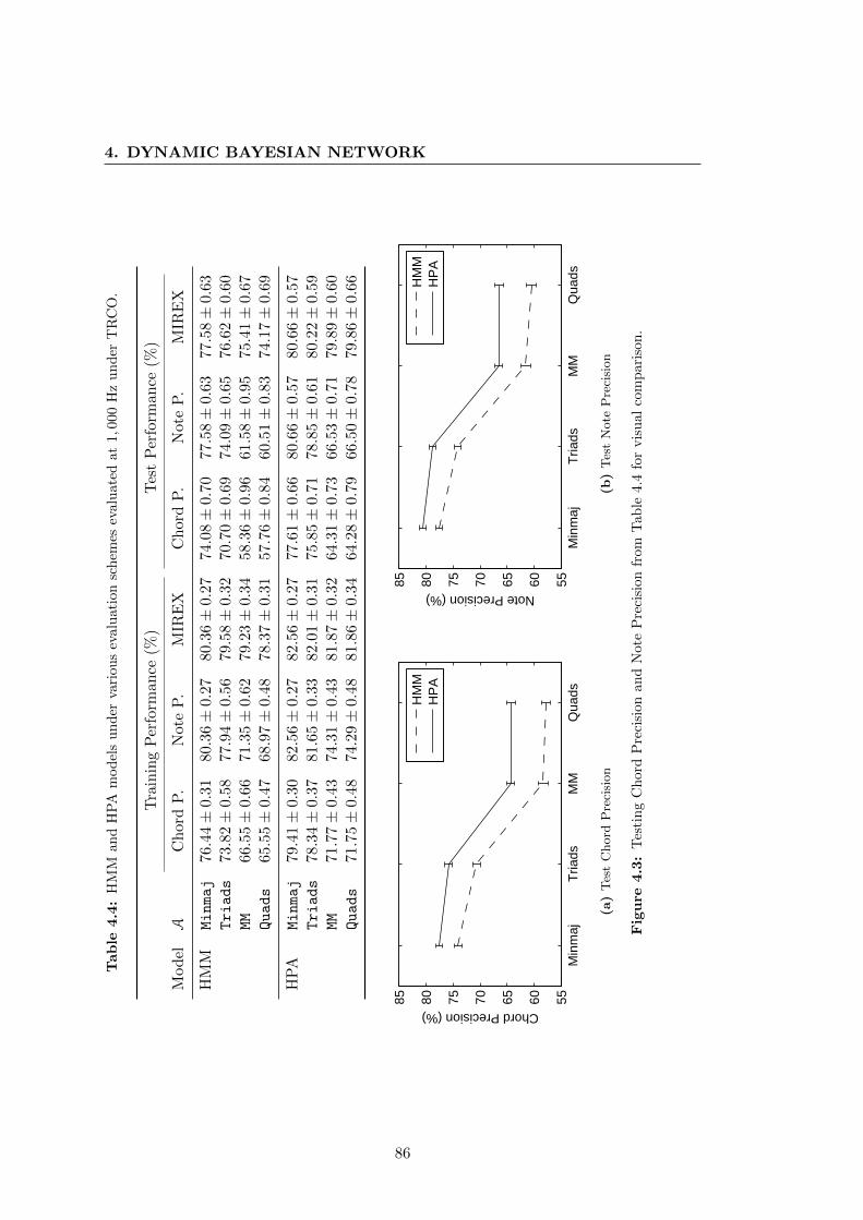
4. DYNAMIC BAYESIAN NETWORK
Tab
le4.4
:H
MM
and
HP
Am
od
els
un
der
vari
ou
sev
alu
ati
on
sch
emes
evalu
ate
dat
1,0
00
Hz
un
der
TR
CO
.
Tra
inin
gP
erfo
rman
ce(%
)T
est
Per
form
ance
(%)
Mod
elA
Ch
ord
P.
Not
eP
.M
IRE
XC
hor
dP
.N
ote
P.
MIR
EX
HM
MMinmaj
76.4
4±
0.31
80.3
6±
0.2
780.3
6±
0.2
774.0
8±
0.7
077.5
8±
0.6
377.5
8±
0.6
3Triads
73.8
2±
0.5
877.9
4±
0.5
679.5
8±
0.3
270.7
0±
0.6
974.0
9±
0.6
576.6
2±
0.6
0MM
66.5
5±
0.6
671.3
5±
0.6
279.2
3±
0.3
458.3
6±
0.9
661.5
8±
0.9
575.4
1±
0.6
7Quads
65.5
5±
0.4
768.9
7±
0.4
878.3
7±
0.3
157.7
6±
0.8
460.5
1±
0.8
374.1
7±
0.6
9
HP
AMinmaj
79.4
1±
0.30
82.5
6±
0.2
782.5
6±
0.2
777.6
1±
0.6
680.6
6±
0.5
780.6
6±
0.5
7Triads
78.3
4±
0.3
781.6
5±
0.3
382.0
1±
0.3
175.8
5±
0.7
178.8
5±
0.6
180.2
2±
0.5
9MM
71.7
7±
0.4
374.3
1±
0.4
381.8
7±
0.3
264.3
1±
0.7
366.5
3±
0.7
179.8
9±
0.6
0Quads
71.7
5±
0.4
874.2
9±
0.4
881.8
6±
0.3
464.2
8±
0.7
966.5
0±
0.7
879.8
6±
0.6
6
Min
maj
Tria
dsM
MQ
uads
55606570758085
Chord Precision (%)
H
MM
HP
A
(a)
Tes
tC
hord
Pre
cisi
on
Min
maj
Tria
dsM
MQ
uads
55606570758085
Note Precision (%)
H
MM
HP
A
(b)
Tes
tN
ote
Pre
cisi
on
Fig
ure
4.3
:T
esti
ng
Ch
ord
Pre
cisi
on
an
dN
ote
Pre
cisi
on
from
Tab
le4.4
for
vis
ual
com
pari
son
.
86
4.3 Complex Chords and Evaluation Strategies
The first observation we can make from Table 4.4 is that HPA outperforms an HMM
in all cases, with non-overlapping error bars of 1 standard deviation. This confirms
HPA’s superiority under all evaluation schemes and chord alphabets. Secondly, we
notice that performance of all types decreases as the chord alphabet increases in size
from minmaj (25 classes) to Quads (133 classes), as expected. Performance drops most
sharply when moving from Triads to MM, possibly owing to the inclusion of 7th chords
and their potential confusion with their constituent triads.
Comparing the different evaluation schemes, we see that Chord Precision is always
lower than Note Precision (as expected), and that the gap between an HMM and HPA
increases as the chord alphabet increases (3.52%−6.52% Chord Precision, 3.08%−5.99%
Note Precision), and is also largest for the Chord Precision metric, confirming that HPA
is more applicable to challenging chord recognition tasks with large chord alphabets
and when evaluation is most stringent.
A brief survey of the MIREX evaluation strategy shows relatively little variation
across models, highlighting a drawback of this evaluation: more complex models are
not “rewarded” for correctly identifying complex chords and/or bass notes. However,
it does allow us to compare HPA to the most recent MIREX evaluation.
Performance under the MIREX evaluation shows that under a train/test scenario,
HPA obtains 80.66±0.57% TRCO (row 5 and final column of Table 4.4), which is to be
compared with Cho and Bello’s submission to MIREX 2011 (Submission CB3 in Table
2.7), which scored 80.91%. Although we have already highlighted the weaknesses of the
MIREX evaluations in the current section and in chapter 2, it is still clear that HPA
performs at a similar level to the cutting edge. The p−values under a paired t−test
for an HMM vs HPA, under all alphabets, the Note Precision and Chord Precision
metrics revealed a maximal value of 3.33 × 10−83, suggesting that HPA significantly
outperforms an HMM in all of these scenarios.
We also ran HPA in a train/train setting on the MIREX dataset, and found it to
87
4. DYNAMIC BAYESIAN NETWORK
perform at 82.45% TRCO, comparable in magnitude to Khadkevich and Olmologo’s
KO1 submission, which attained 82.85% TRCO (see Table 2.7).
4.4 Conclusions
In this chapter, we revealed our Dynamic Bayesian Network, the Harmony Progression
Analyser (HPA). We formulated HPA mathematically as Viterbi decoding of a pair
of bass and treble chromagrams in a similar way to an HMM, but on a larger state
space consisting of hidden nodes for chord, bass and key sequences. We noted that
this increase in state space has a drawback: computational time increases significantly,
and we introduced machine-learning based techniques (two-stage prediction, dynamic
pruning) to select a subspace of the parameter space to explore.
Next, we tested the accuracy of HPA by gradually increasing the number of nodes,
and found that each additional node statistically significantly increased performance in
a train/test setting. Bass note accuracy peaked at 85.71% TRCO, which was investi-
gated by studying both Chord Precision and Note Precision in the evaluation section
using a complex chord alphabet, where we attained results comparable to the state of
the art.
88

5
Exploiting Additional Data
We have seen that our Dynamic Bayesian Network HPA is able to perform at a cutting-
edge level when trained and evaluated on a known set of 217 popular music tracks.
However, one of the main benefits of designing a machine-learning based system is that
it may be retrained on new data as it arises.
Recently, a number of new fully-labelled chord sequence annotations have been made
available. These include the USpop set of 194 tracks [7] and the Billboard dataset of
1,000 tracks, for which the ground truth has been released for 649 (the remainder
being saved for test data in future MIREX evaluations) [13]. We may also make use of
seven Carole King annotations1 and a collection of five tracks by the rock group, Oasis,
curated by ourselves [74].
In addition to these fully-labelled datasets, we have access to Untimed Chord Se-
quences (UCSs, see section 5.4) for a subset of the MIREX and Billboard datasets, as
well as for an additional set of 1, 822 songs. Such UCSs have been shown by ourselves
in the past to improve chord recognition when training data is limited [73].
There are many ways of combining the data mentioned above, and an almost limit-
less number of experiments we could perform with the luxury of these newly available
1obtained with thanks from http://isophonics.net/
89
5. EXPLOITING ADDITIONAL DATA
training sources. To retain our focus we will structure the experiments in this chapter
to investigate the following questions:
1. How similar are the datasets to each other?
2. Can we learn from one of the datasets to test in another (a process known as out
of domain testing)?
3. How do an HMM and HPA compare in each of the above settings?
4. Are any sets similar enough to be combined into one unified training set?
5. How fast does HPA learn?
6. Can we use Untimed Chord Sequences as an additional source of information in
a test setting?
7. Can a large number of UCSs be used as an additional source of training data?
We will answer the above questions in this chapter by following the following struc-
ture. Section 5.1 will investigate the similarity between datasets and aims to see if
testing out of domain is possible, answering points 1-3 above. Section 5.2 briefly in-
vestigates point 4 by using leave-one-out testing on all songs for which we have key
annotations, whilst learning rates (point 5) are studied in section 5.3. The mathemat-
ical framework for using chord databases as an additional data source is introduced in
section 5.4 (point 6). We then move on to see how these data may be used in training
in section 5.5 (point 7) before concluding the chapter in section 5.6.
5.1 Training across different datasets
Machine-learning approaches to a recognition task require training data to learn map-
pings from features to classes. Such training data may come from varying distributions,
which may affect the type of model learnt, and also the generalisation of the model.
90
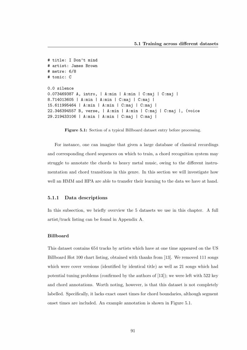
5.1 Training across different datasets
# title: I Don’t mind
# artist: James Brown
# metre: 6/8
# tonic: C
0.0 silence
0.073469387 A, intro, | A:min | A:min | C:maj | C:maj |
8.714013605 | A:min | A:min | C:maj | C:maj |
15.611995464 | A:min | A:min | C:maj | C:maj |
22.346394557 B, verse, | A:min | A:min | C:maj | C:maj |, (voice
29.219433106 | A:min | A:min | C:maj | C:maj |
Figure 5.1: Section of a typical Billboard dataset entry before processing.
For instance, one can imagine that given a large database of classical recordings
and corresponding chord sequences on which to train, a chord recognition system may
struggle to annotate the chords to heavy metal music, owing to the different instru-
mentation and chord transitions in this genre. In this section we will investigate how
well an HMM and HPA are able to transfer their learning to the data we have at hand.
5.1.1 Data descriptions
In this subsection, we briefly overview the 5 datasets we use in this chapter. A full
artist/track listing can be found in Appendix A.
Billboard
This dataset contains 654 tracks by artists which have at one time appeared on the US
Billboard Hot 100 chart listing, obtained with thanks from [13]. We removed 111 songs
which were cover versions (identified by identical title) as well as 21 songs which had
potential tuning problems (confirmed by the authors of [13]); we were left with 522 key
and chord annotations. Worth noting, however, is that this dataset is not completely
labelled. Specifically, it lacks exact onset times for chord boundaries, although segment
onset times are included. An example annotation is shown in Figure 5.1.
91
5. EXPLOITING ADDITIONAL DATA
Although section starts are time-stamped, exact chord onset times are not present.
To counteract this, we extracted chord labels directly from the text and aligned them
to the corresponding chromagram (many thanks to Ashley Burgoyne for running our
feature extraction software on the music source), assuming that each bar has equal
duration. This process was repeated for the key annotations to yield a set of annotations
in the style of Harte et al. [36].
MIREX
The MIREX dataset, as mentioned in previous chapters, contains 218 tracks with 180
songs by The Beatles, 20 by Queen and 18 by Zweieck. We omitted “Revolution Number
9” from the dataset as it was judged to have no meaningful harmonic content, and were
left with 217 chord and key annotations.
USpop
This dataset of 194 tracks has only very recently been made available, and is sampled
from the USpop2002 dataset of 8,752 songs [7]. Full chord labels are available, although
there is no data on key labels for these songs, meaning they unfortunately cannot be
used to train HPA. Despite this, we may train an HMM on these data, or use them
exclusively for testing purposes.
Carole King
A selection of seven songs by the folk/rock singer Carole King, with corresponding key
annotations. Although these annotations come from the same source as the MIREX
datasets, we do not include them in the MIREX dataset, as they are not included in
the MIREX evaluation and their quality is disputed1.
1quote from isophonics.net: [...the annotations] have not been carefully checked, use with care.
92
5.1 Training across different datasets
Oasis
A small set of five songs by the Britpop group Oasis, made by ourselves for one of
our previous publications [74]. These data are not currently complemented by key
annotations.
5.1.2 Experiments
In this subsection we will train an HMM and HPA on the sets of chord and (for HPA)
key annotations, and test on the remaining sets of data to investigate how flexible our
model is, and how much learning may be transferred from one dataset to another.
Unfortunately, we cannot train HPA on the USpop or Oasis datasets as they lack
key information. Therefore, we begin by deploying an HMM on all datasets. Results are
shown in Table 5.1, where we evaluated using Chord Precision and Note Precision; and
utilised TRCO as the overall evaluation metric, sampled at 1, 000 Hz, using all chord
alphabets from the previous chapter. Results for Chord Precession are also shown in
Figure 5.2.
93
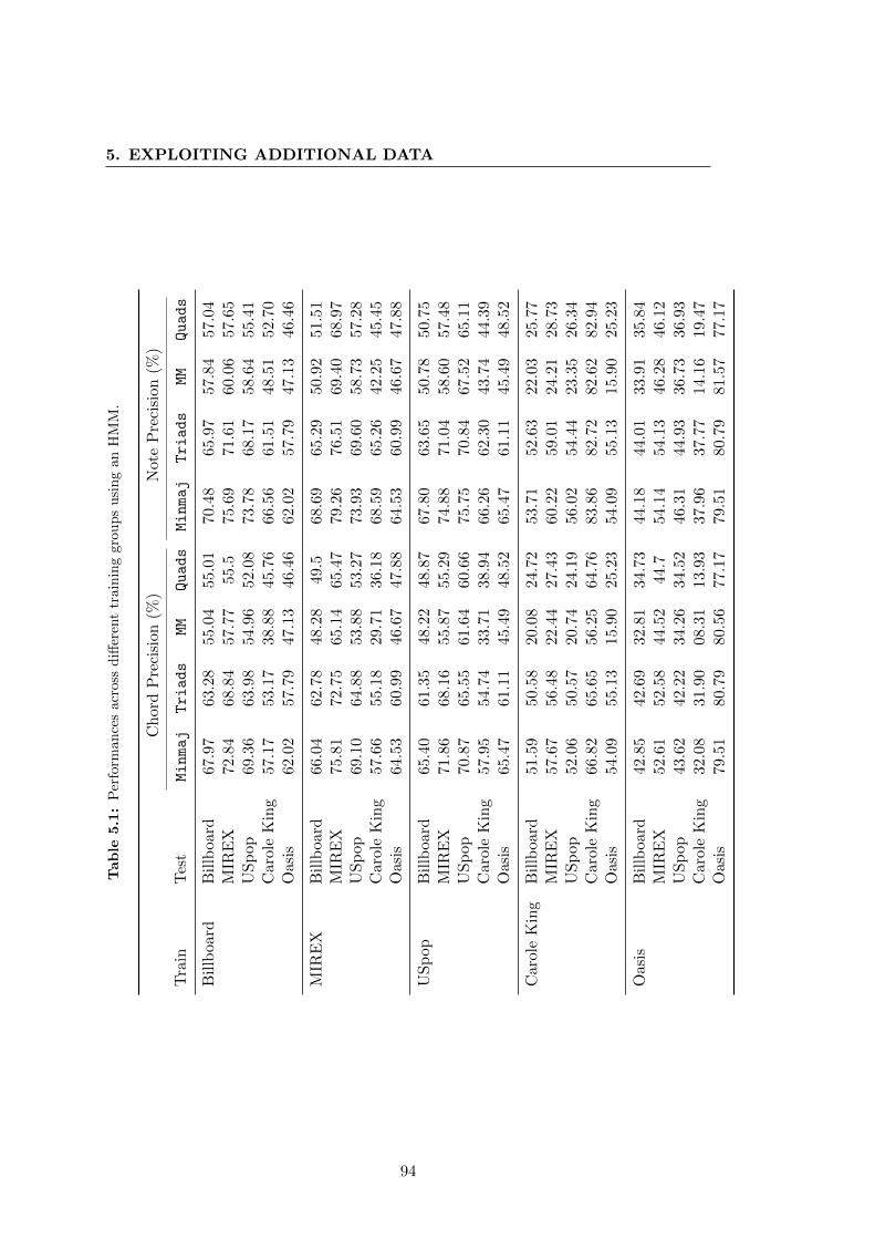
5. EXPLOITING ADDITIONAL DATA
Tab
le5.1
:P
erfo
rman
ces
acr
oss
diff
eren
ttr
ain
ing
gro
up
su
sin
gan
HM
M.
Ch
ord
Pre
cisi
on(%
)N
ote
Pre
cisi
on(%
)
Tra
inT
est
Minmaj
Triads
MM
Quads
Minmaj
Triads
MM
Quads
Bil
lboa
rdB
illb
oard
67.9
763.2
855.0
455.0
170.4
865.9
757.8
457.0
4M
IRE
X72.8
468.8
457.7
755.5
75.6
971.6
160.0
657.6
5U
Sp
op69.3
663.9
854.9
652.0
873.7
868.1
758.6
455.4
1C
arol
eK
ing
57.1
753.1
738.8
845.7
666.5
661.5
148.5
152.7
0O
asis
62.0
257.7
947.1
346.4
662.0
257.7
947.1
346.4
6
MIR
EX
Bil
lboa
rd66.0
462.7
848.2
849.5
68.6
965.2
950.9
251.5
1M
IRE
X75.8
172.7
565.1
465.4
779.2
676.5
169.4
068.9
7U
Sp
op69.1
064.8
853.8
853.2
773.9
369.6
058.7
357.2
8C
arol
eK
ing
57.6
655.1
829.7
136.1
868.5
965.2
642.2
545.4
5O
asis
64.5
360.9
946.6
747.8
864.5
360.9
946.6
747.8
8
US
pop
Bil
lboa
rd65.4
061.3
548.2
248.8
767.8
063.6
550.7
850.7
5M
IRE
X71.8
668.1
655.8
755.2
974.8
871.0
458.6
057.4
8U
Sp
op70.8
765.5
561.6
460.6
675.7
570.8
467.5
265.1
1C
arol
eK
ing
57.9
554.7
433.7
138.9
466.2
662.3
043.7
444.3
9O
asis
65.4
761.1
145.4
948.5
265.4
761.1
145.4
948.5
2
Car
ole
Kin
gB
illb
oard
51.5
950.5
820.0
824.7
253.7
152.6
322.0
325.7
7M
IRE
X57.6
756.4
822.4
427.4
360.2
259.0
124.2
128.7
3U
Sp
op52.0
650.5
720.7
424.1
956.0
254.4
423.3
526.3
4C
arol
eK
ing
66.8
265.6
556.2
564.7
683.8
682.7
282.6
282.9
4O
asis
54.0
955.1
315.9
025.2
354.0
955.1
315.9
025.2
3
Oas
isB
illb
oard
42.8
542.6
932.8
134.7
344.1
844.0
133.9
135.8
4M
IRE
X52.6
152.5
844.5
244.7
54.1
454.1
346.2
846.1
2U
Sp
op43.6
242.2
234.2
634.5
246.3
144.9
336.7
336.9
3C
arol
eK
ing
32.0
831.9
008.3
113.9
337.9
637.7
714.1
619.4
7O
asis
79.5
180.7
980.5
677.1
779.5
180.7
981.5
777.1
7
94

5.1 Training across different datasets
We immediately see a large variation in the performances from Table 5.1 (8.31%−
79.51% Chord Precision and 14.16%−79.51% Note Precision). Worth noting, however,
is that these extreme values are seen when there are few training examples (training
set Carole King or Oasis). In such cases, when the training and test sets coincide, it
is easy for the model to overfit the model (shown by high performances in train/test
Oasis and Carole King), whilst generalisation is poor (low performances when testing on
Billboard/MIREX/USpop). This is due to the model lacking the necessary information
to train the hidden or observed chain. It is extremely unlikely, for example, that the
full range of Quads chords are seen in the Oasis dataset, meaning that these chords are
rarely decoded by the Viterbi algorithm (although small pseudocounts of 1 chord were
used to try to counteract this).
These extreme cases highlight the dependence of machine-learning based systems
on a large amount of good quality training data. When testing on the small datasets
(Carole King and Oasis), this becomes even more of an issue, in the most extreme case
giving a training set performance of 81.57% and test set performance of 14.16% (test
artist Carole King, MM chord alphabet).
In cases where we have sufficient data however (train sets Billboard, MIREX and
USpop), we see more encouraging results (worst performance at minmaj was 65.40%
when training on USpop, testing on Billboard). Performance in TRCO generally de-
creases as the alphabet size increases as expected, with the sharpest decrease occurring
from the Triads alphabet to MM. We also see that each performance is highest when
the training/testing data coincide, as expected, and that this is more pronounced as
the chord alphabet increases in complexity. Training/testing performances for the Bill-
board, MIREX and USpop datasets appear to be quite similar (at most 11.46% differ-
ence in Chord Precision and minmaj alphabet, 10.41% for Note Precision), suggesting
that these data may be combined to give a larger training set.
We now move on to see how HPA deals with the variance across datasets. Since
95
5. EXPLOITING ADDITIONAL DATA
we require key annotations for training HPA, we shall restrict ourselves here to the
Billboard, MIREX and Carole King datasets. Results are shown in Table 5.2 and
Figure 5.3. We also show comparative plots between an HMM and HPA in Figure 5.4.
96
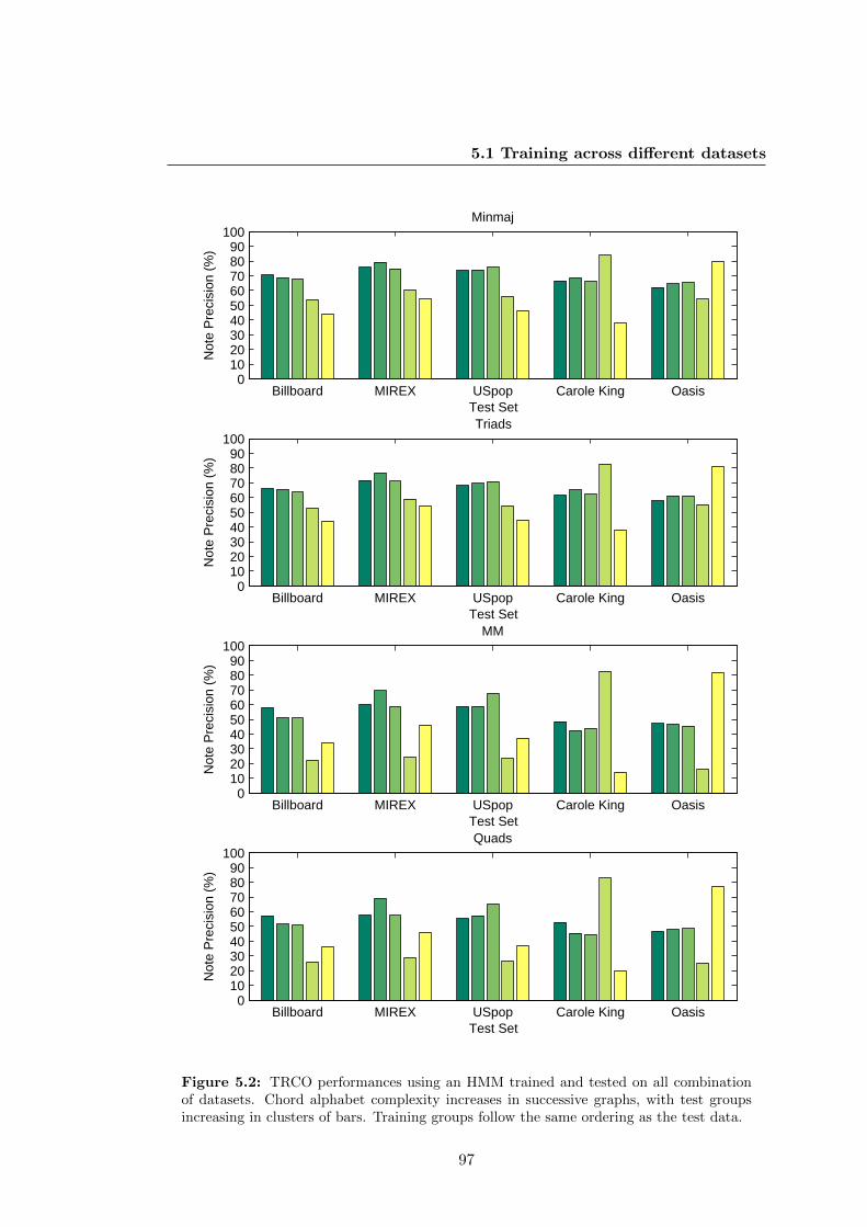
5.1 Training across different datasets
Billboard MIREX USpop Carole King Oasis0
102030405060708090
100
Test Set
Not
e P
reci
sion
(%
)Minmaj
Billboard MIREX USpop Carole King Oasis0
102030405060708090
100
Test Set
Not
e P
reci
sion
(%
)
Triads
Billboard MIREX USpop Carole King Oasis0
102030405060708090
100
Test Set
Not
e P
reci
sion
(%
)
MM
Billboard MIREX USpop Carole King Oasis0
102030405060708090
100
Test Set
Not
e P
reci
sion
(%
)
Quads
Figure 5.2: TRCO performances using an HMM trained and tested on all combinationof datasets. Chord alphabet complexity increases in successive graphs, with test groupsincreasing in clusters of bars. Training groups follow the same ordering as the test data.
97
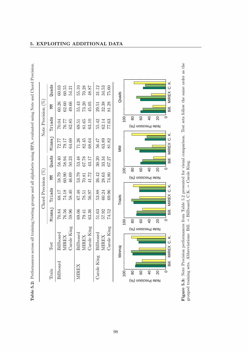
5. EXPLOITING ADDITIONAL DATA
Tab
le5.2
:P
erfo
rman
ces
acro
ssal
ltr
ain
ing/
test
ing
gro
up
san
dall
alp
hab
ets
usi
ng
HP
A,ev
alu
ate
du
sin
gN
ote
an
dC
hord
Pre
cisi
on
.
Ch
ord
Pre
cisi
on(%
)N
ote
Pre
cisi
on(%
)
Tra
inT
est
Minmaj
Triads
MM
Quads
Minmaj
Triads
MM
Quads
Bil
lboa
rdB
illb
oard
70.8
468.1
758.7
958.4
072.7
770.0
460.2
660.0
3M
IRE
X76.5
674.1
860.9
058.9
479.1
776.7
762.6
060.5
5C
arol
eK
ing
59.9
658.4
046.6
950.2
364.6
062.8
549.6
654.2
1
MIR
EX
Bil
lboa
rd69.0
667.4
853.7
953.4
871.2
669.5
155.4
355.1
0M
IRE
X79.4
178.5
170.8
167.7
882.4
581.6
573.2
070.2
8C
arol
eK
ing
63.3
656.9
741.7
243.1
768.6
463.1
045.0
548.8
7
Car
ole
Kin
gB
illb
oard
51.6
353.8
826.4
230.2
056.4
755.4
229.5
131.1
2M
IRE
X57.9
260.2
428.6
333.3
463.8
962.1
432.3
834.5
3C
arol
eK
ing
74.5
269.9
674.8
067.2
781.8
277.6
381.2
875.6
0
Bill
.M
IRE
XC
. K.
020406080100
Note Precision (%)
Min
maj
Bill
.M
IRE
XC
. K.
020406080100
Note Precision (%)T
riads
Bill
.M
IRE
XC
. K.
020406080100
Note Precision (%)
MM
Bill
.M
IRE
XC
. K.
020406080100
Note Precision (%)
Qua
ds
Fig
ure
5.3
:N
ote
Pre
cisi
onp
erfo
rman
ces
from
Tab
le5.2
pre
sente
dfo
rvis
ual
com
pari
son
.T
est
sets
foll
owth
esa
me
ord
eras
the
grou
ped
trai
nin
gse
ts.
Ab
bre
via
tion
s:B
ill.
=B
illb
oard
,C
.K.
=C
aro
leK
ing.
98
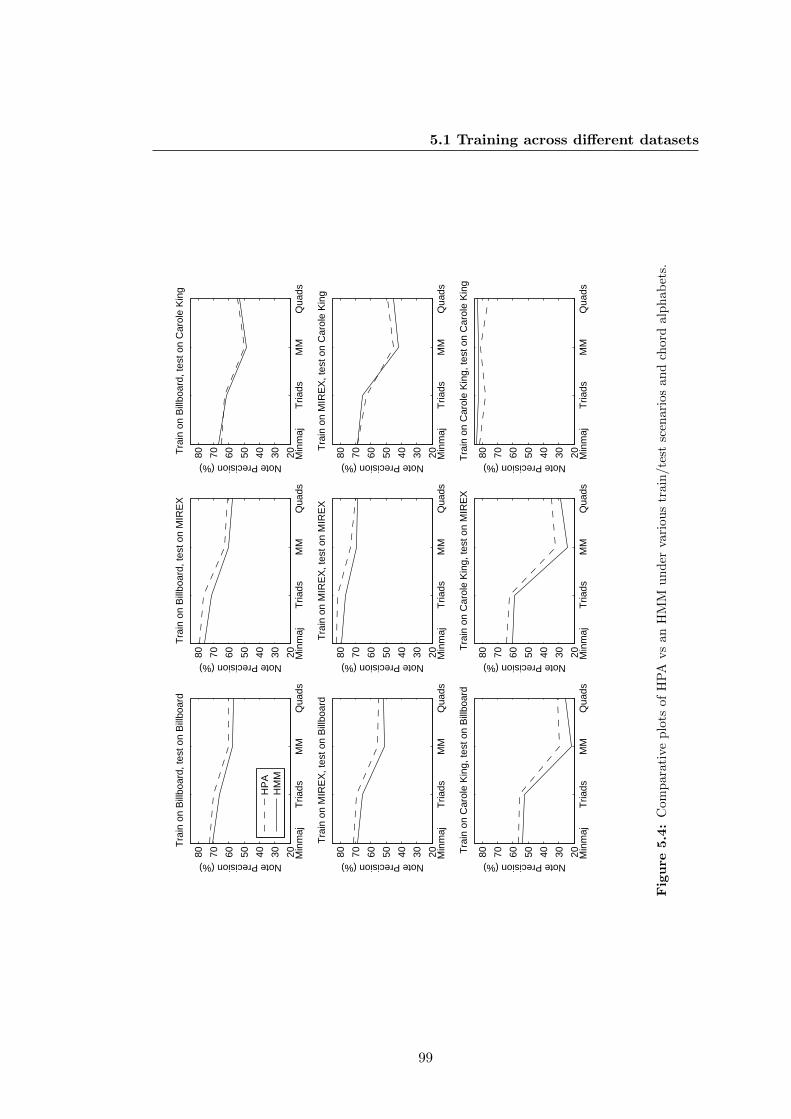
5.1 Training across different datasets
Min
maj
Tria
dsM
MQ
uads
20304050607080
Note Precision (%)
Tra
in o
n B
illbo
ard,
test
on
Bill
boar
d
HP
AH
MM
Min
maj
Tria
dsM
MQ
uads
20304050607080
Note Precision (%)
Tra
in o
n B
illbo
ard,
test
on
MIR
EX
Min
maj
Tria
dsM
MQ
uads
20304050607080
Note Precision (%)
Tra
in o
n B
illbo
ard,
test
on
Car
ole
Kin
g
Min
maj
Tria
dsM
MQ
uads
20304050607080
Note Precision (%)
Tra
in o
n M
IRE
X, t
est o
n B
illbo
ard
Min
maj
Tria
dsM
MQ
uads
20304050607080
Note Precision (%)
Tra
in o
n M
IRE
X, t
est o
n M
IRE
X
Min
maj
Tria
dsM
MQ
uads
20304050607080
Note Precision (%)
Tra
in o
n M
IRE
X, t
est o
n C
arol
e K
ing
Min
maj
Tria
dsM
MQ
uads
20304050607080
Note Precision (%)
Tra
in o
n C
arol
e K
ing,
test
on
Bill
boar
d
Min
maj
Tria
dsM
MQ
uads
20304050607080
Note Precision (%)T
rain
on
Car
ole
Kin
g, te
st o
n M
IRE
X
Min
maj
Tria
dsM
MQ
uads
20304050607080
Note Precision (%)Tra
in o
n C
arol
e K
ing,
test
on
Car
ole
Kin
g
Fig
ure
5.4
:C
omp
arat
ive
plo
tsof
HP
Avs
an
HM
Mu
nd
erva
riou
str
ain
/te
stsc
enari
os
an
dch
ord
alp
hab
ets.
99
5. EXPLOITING ADDITIONAL DATA
Comparing results for HPA with those for HMM, we see an improvement in almost
all cases, although when testing on the small set of Carole King it is difficult to tell which
method is best. The effect of overfitting on limited training data is most obviously seen
in Figure 5.4, bottom row. When training and testing on Carole King (lower right),
an HMM is able to attain above 80% on all chord alphabets. However, testing these
parameters on the Billboard or MIREX datasets (lower left and lower centre of Figure
5.4), performance does not exceed 65%.
In contrast to this, the Billboard and MIREX datasets offer more comparable per-
formances under train/test. Indeed, the largest difference between train and test per-
formances under the minmaj alphabet is at most 11.2% (train/test on MIREX vs train
on Billboard, test on MIREX). It is also encouraging to see that by training on the
Billboard data, we attain higher performance when testing on MIREX (76.56% minmaj
Chord Precision) than when testing on the Billboard dataset itself (70.84%), as this
means we may combine these datasets to form a large training set.
5.2 Leave one out testing
Before moving on to discuss the learning rate of HPA, we digress to a simple experiment
to test if all annotations with key annotations may be combined to form a large training
set. One method is to test on each data point, with the training set consisting of all
other examples, a process known as “leave-one-out” testing [48]. Results for these
experiments are shown in Table 5.3 and Figure 5.5.
100
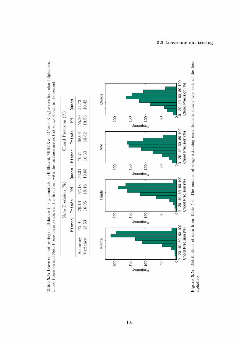
5.2 Leave one out testingT
ab
le5.3
:L
eave
-on
e-ou
tte
stin
gon
alld
ata
wit
hke
yan
nota
tion
s(B
illb
oard
,M
IRE
Xan
dC
aro
leK
ing)
acr
oss
four
chord
alp
hab
ets.
Ch
ord
Pre
cisi
onan
dN
ote
Pre
cisi
onar
esh
own
inth
efi
rst
row
,w
ith
the
vari
an
ceacr
oss
test
son
gs
show
nin
the
seco
nd
.
Not
eP
reci
sion
(%)
Ch
ord
Pre
cisi
on(%
)
Minmaj
Triads
MM
Quads
Minmaj
Triads
MM
Quads
Acc
ura
cy72.9
170.1
657.1
856.3
170.7
168.0
655.7
054.7
3V
aria
nce
15.5
316.0
619.1
619.0
516.3
016.8
219.5
319.4
2
020
4060
8010
0050100
150
200
Cho
rd P
reci
sion
(%
)
Frequency
Min
maj
020
4060
8010
0050100
150
200
Cho
rd P
reci
sion
(%
)
Frequency
Tria
ds
020
4060
8010
0050100
150
200
Cho
rd P
reci
sion
(%
)
Frequency
MM
020
4060
8010
0050100
150
200
Cho
rd P
reci
sion
(%
)
Frequency
Qua
ds
Fig
ure
5.5
:D
istr
ibu
tion
sof
dat
afr
omT
able
5.3
.T
he
nu
mb
erof
son
gs
att
ain
ing
each
dec
ile
issh
own
over
each
of
the
fou
ral
ph
abet
s.
101
5. EXPLOITING ADDITIONAL DATA
Leave one out testing offers a trade-off between the benefit of a large training size
and the high variance of the prediction accuracies. The relatively high performances
seen in this setting of 70.84% Chord Precision shows that the MIREX and Billboard
datasets are fairly similar, although the variance is large, as expected from a leave-
one-out setting. Upon inspecting the histograms in Figure 5.5, we see that most songs
perform at around 60− 80% Chord Precision for the minmaj alphabet with a positive
skew. The variance across songs is shown by the width of the histograms, highlighting
the range of difficulty in prediction across this dataset.
5.3 Learning Rates
We have seen that it is possible to train HPA under various circumstances and attain
good performance under a range of training/test schemes. However, an important
question that remains to be answered is how quickly HPA learns from training data.
The current section will address this concern by incrementally increasing the amount
of training data that HPA is exposed to.
5.3.1 Experiments
The experiments for this section will follow that of 5.2, using HPA on all songs with
key annotations. We saw in this section that combining these datasets offers good per-
formance when using leave-one-out testing, although the variance was large. However,
in the Billboard dataset, the number of songs is sufficiently large (522) that we may
perform train-test experiments. Instead of using a fixed ratio of train to test, we will
increase the training ratio to see how fast HPA and an HMM learn.
This is obtained by partitioning the set of 522 songs into disjoint subsets of increas-
ing size, with the remainder being held out for testing. Since there are many ways
to do this, the process is repeated many times to assess variance. We chose training
102
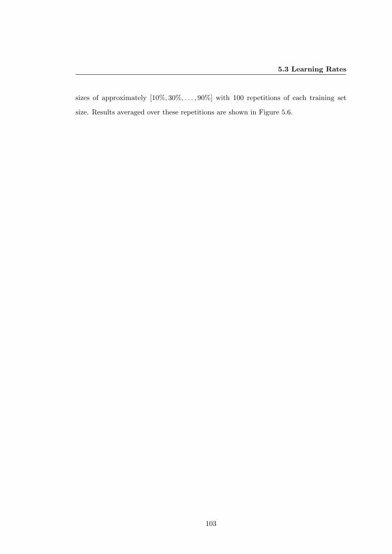
5.3 Learning Rates
sizes of approximately [10%, 30%, . . . , 90%] with 100 repetitions of each training set
size. Results averaged over these repetitions are shown in Figure 5.6.
103
5. EXPLOITING ADDITIONAL DATA
1030
5070
906768697071727374
Min
maj
Tra
inin
g si
ze (
%)
Note Precision
1030
5070
9065666768697071
Tria
ds
Tra
inin
g si
ze (
%)
Note Precision
1030
5070
90484950515253545556575859
MM
Tra
inin
g si
ze (
%)
Note Precision
1030
5070
90474849505152535455565758
Qua
ds
Tra
inin
g si
ze (
%)
Note Precision
1030
5070
90656667686970717273
Min
maj
Tra
inin
g si
ze (
%)
Chord Precision
1030
5070
906364656667686970
Tria
ds
Tra
inin
g si
ze (
%)
Chord Precision
1030
5070
9046474849505152535455565758
MM
Tra
inin
g si
ze (
%)
Chord Precision
1030
5070
9045464748495051525354555657
Qua
ds
Tra
inin
g si
ze (
%)
Chord Precision
Fig
ure
5.6
:L
earn
ing
rate
ofH
PA
wh
enu
sin
gin
crea
sin
gam
ou
nts
of
the
Bil
lboard
data
set.
Tra
inin
gsi
zein
crea
ses
alo
ng
thex
axis
,w
ith
eith
erN
ote
orC
hor
dP
reci
sion
mea
sure
don
they
axis
.E
rror
bars
of
wid
th1
stan
dard
dev
iati
on
acr
oss
the
ran
dom
isati
on
sar
eal
sosh
own
.
104
5.4 Chord Databases for use in testing
5.3.2 Discussion
Generally speaking, we see from Figure 5.6 that test performance improves as the
amount of data increases. Performance increases about 2.5 percentage points for the
minmaj alphabet, and around 4 percentage points for the MM/Quads alphabet. The
performance for the Triads alphabet appears to plateau very quickly to 65%, with
manual inspection revealing that the performance increased very rapidly from 0 to
10% training size. In all cases the increase slightly more pronounced under the Chord
Precision evaluation, which we would expect as it is the more challenging evaluation
and benefits the most from additional data.
5.4 Chord Databases for use in testing
Owing to the scarcity of fully labelled data until very recent times, some authors have
explored other sources of information to train models, as we have done in our previous
work [60, 72, 73, 74]. One such source of information is guitarist websites such as e-
chords1. These websites typically include chord labels and lyrics annotated for many
thousands of songs. In the present section we will investigate if such websites can be
used to aid chord recognition, following our previous work in the area [74].
5.4.1 Untimed Chord Sequences
e-chords.com is a website where registered users are able to upload the chords, lyrics,
keys, and structural information for popular songs2. Although the lyrics may provide
useful information, we discard them in the current analysis.
Some e-chords annotations contain key information, although informal investiga-
tions have led us to believe that this information is highly noisy, so it will be discarded
1www.e-chords.com2although many websites similar to e-chords exist, we chose to work with this owing to its size
(annotations for over 140, 000 songs) and the ease of extraction (chord labels are enclosed in html tags,making them easy to robustly “scrape” from the web).
105
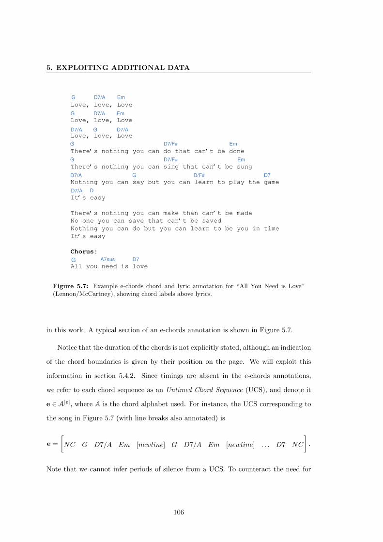
5. EXPLOITING ADDITIONAL DATA
Love, Love, Love
Love, Love, Love
Love, Love, Love
There’s nothing you can do that can’t be done
There’s nothing you can sing that can’t be sung
Nothing you can say but you can learn to play the game
It’s easy
There’s nothing you can make than can’t be made
No one you can save that can’t be saved
Nothing you can do but you can learn to be you in time
It’s easy
Chorus:
All you need is love
G D7/A Em
G D7/A Em
D7/A G D7/A
G D7/F# Em
G D7/F# Em
D7/A G D/F# D7
D7/A D
G A7sus D7
Figure 5.7: Example e-chords chord and lyric annotation for “All You Need is Love”(Lennon/McCartney), showing chord labels above lyrics.
in this work. A typical section of an e-chords annotation is shown in Figure 5.7.
Notice that the duration of the chords is not explicitly stated, although an indication
of the chord boundaries is given by their position on the page. We will exploit this
information in section 5.4.2. Since timings are absent in the e-chords annotations,
we refer to each chord sequence as an Untimed Chord Sequence (UCS), and denote it
e ∈ A|e|, where A is the chord alphabet used. For instance, the UCS corresponding to
the song in Figure 5.7 (with line breaks also annotated) is
e =
[NC G D7/A Em [newline] G D7/A Em [newline] . . . D7 NC
].
Note that we cannot infer periods of silence from a UCS. To counteract the need for
106

5.4 Chord Databases for use in testing
silence at the beginning and end of songs, we added a no-chord symbol at the start and
end of each UCS.
It is worth noting that multiple versions of some songs exist. A variation may have
different but similar-sounding chord sequences (we assume the annotations on e-chords
are uploaded by people without formal musical training), different recordings of the
same song, or in a transposed key (the last of these is common because some keys on
the guitar are easier to play in than others). We refer to the multiple files as song
redundancies, and to be exhaustive we consider each of the redundancies in every key
transposition. We will discuss a way of choosing the best key and redundancy in section
5.4.3.
The principle of this section is to use the UCSs to constrain, in a certain way, the
set of possible chord transitions for a given test song. Mathematically, this is done by
modelling the joint probability of chords and chromagrams of a song (X,y) by
P ′(X,y|Θ, e) = Pini(y1|Θ) · Pobs(x1|y1,Θ) ·|y|∏t=2
P ′tr(yt|yt−1,Θ, e) · Pobs(xt|yt,Θ). (5.1)
This distribution is the same as in Equation 2.11, except that the transition distribution
P ′tr now also depends on the e-chord UCS e for this song, essentially by constraining
the transitions that are allowed, as we will detail in subsection 5.4.2.
An important benefit of this approach is that the chord recognition task can still be
solved by the Viterbi algorithm, albeit applied to an altered model with an augmented
transition probability distribution. Chord recognition using the extra information from
the UCS then amounts to solving
y∗ = arg maxy
P ′(X,y|Θ, e). (5.2)
The more stringent the constraints imposed on P ′tr, the more information from the UCS
is used, but the effect of noise will be more detrimental. On the other hand, if the extent
107
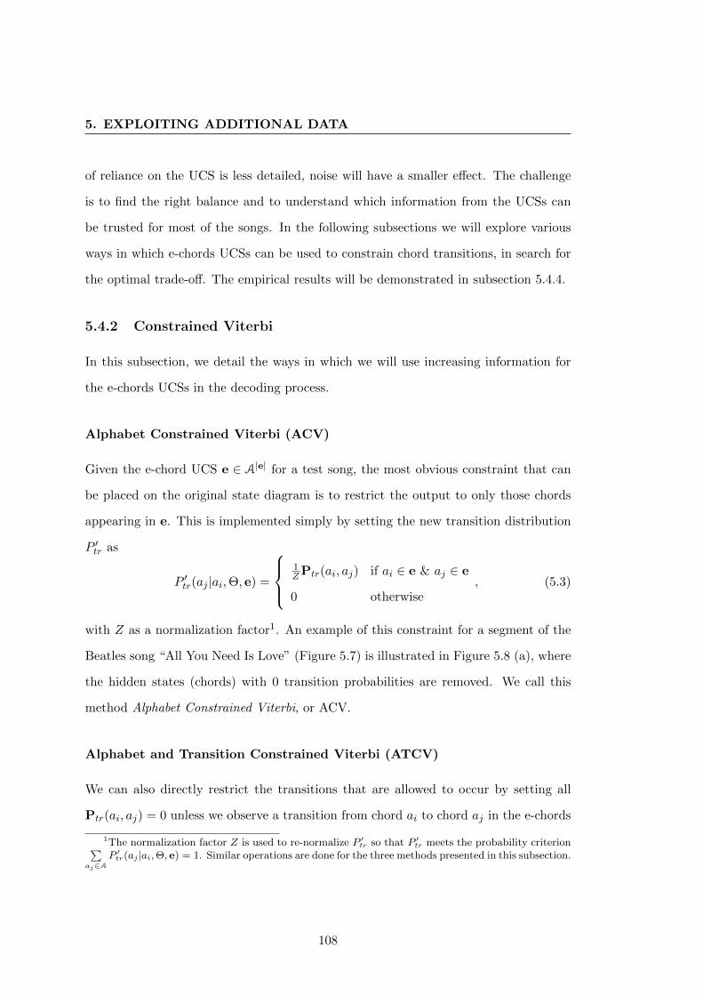
5. EXPLOITING ADDITIONAL DATA
of reliance on the UCS is less detailed, noise will have a smaller effect. The challenge
is to find the right balance and to understand which information from the UCSs can
be trusted for most of the songs. In the following subsections we will explore various
ways in which e-chords UCSs can be used to constrain chord transitions, in search for
the optimal trade-off. The empirical results will be demonstrated in subsection 5.4.4.
5.4.2 Constrained Viterbi
In this subsection, we detail the ways in which we will use increasing information for
the e-chords UCSs in the decoding process.
Alphabet Constrained Viterbi (ACV)
Given the e-chord UCS e ∈ A|e| for a test song, the most obvious constraint that can
be placed on the original state diagram is to restrict the output to only those chords
appearing in e. This is implemented simply by setting the new transition distribution
P ′tr as
P ′tr(aj |ai,Θ, e) =
1ZPtr(ai, aj) if ai ∈ e & aj ∈ e
0 otherwise, (5.3)
with Z as a normalization factor1. An example of this constraint for a segment of the
Beatles song “All You Need Is Love” (Figure 5.7) is illustrated in Figure 5.8 (a), where
the hidden states (chords) with 0 transition probabilities are removed. We call this
method Alphabet Constrained Viterbi, or ACV.
Alphabet and Transition Constrained Viterbi (ATCV)
We can also directly restrict the transitions that are allowed to occur by setting all
Ptr(ai, aj) = 0 unless we observe a transition from chord ai to chord aj in the e-chords
1The normalization factor Z is used to re-normalize P ′tr so that P ′tr meets the probability criterion∑aj∈A
P ′tr(aj |ai,Θ, e) = 1. Similar operations are done for the three methods presented in this subsection.
108
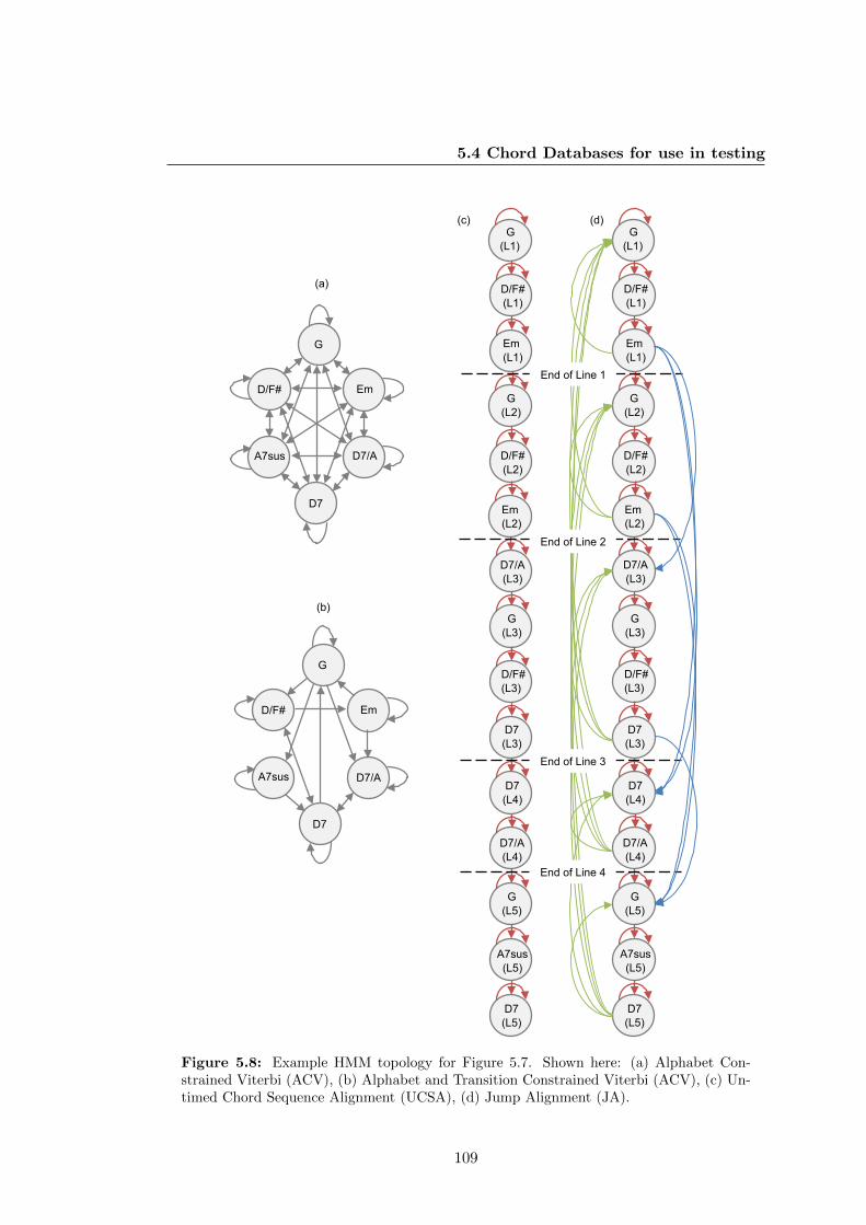
5.4 Chord Databases for use in testing
Em
D7/A A7sus
D/F#
G
D7
Em
D7/A A7sus
D/F#
G
D7
D7 (L3)
D/F# (L3)
A7sus (L5)
G (L5)
D7/A (L4)
D7 (L4)
D7 (L5)
G (L3)
D7/A (L3)
Em (L2)
D/F# (L2)
G (L2)
Em (L1)
D/F# (L1)
G (L1)
D7 (L3)
D/F# (L3)
A7sus (L5)
G (L5)
D7/A (L4)
D7 (L4)
D7 (L5)
G (L3)
D7/A (L3)
Em (L2)
D/F# (L2)
G (L2)
Em (L1)
D/F# (L1)
G (L1)
End of Line 2
End of Line 3
End of Line 4
(a)
(b)
(c) (d)
End of Line 1
Figure 5.8: Example HMM topology for Figure 5.7. Shown here: (a) Alphabet Con-strained Viterbi (ACV), (b) Alphabet and Transition Constrained Viterbi (ACV), (c) Un-timed Chord Sequence Alignment (UCSA), (d) Jump Alignment (JA).
109

5. EXPLOITING ADDITIONAL DATA
file (e.g. Figure 5.8 (b)). This is equivalent to constraining P ′tr such that,
P ′tr(aj |ai,Θ, e) =
1ZPtr(ai, aj) if aiaj ∈ e or ai = ajand ai ∈ e
0 otherwise, (5.4)
where aiaj denotes a transition pair and Z is the normalization factor. We call this
method Alphabet and Transition Constrained Viterbi, ATCV. The topology for this
method is shown in Figure 5.8(b).
Untimed Chord Sequence Alignment (UCSA)
An even more stringent constraint on the chord sequence y for a test song is to require
it to respect the exact order of chords as seen in the UCS e. Doing this corresponds
to finding an alignment of e to the audio, since all that remains for the decoder to do
is ascertain the duration of each chord. In fact, symbolic-to-audio sequence alignment
has previously been exploited as a chord recognition scheme and was shown to achieve
promising results on a small set of Beatles’ and classical music [99], albeit in an ideal
noise-free setting.
Interestingly, sequence alignment can be formalized as Viterbi inference in an HMM
with a special set of states and state transitions (see e.g., the pair-HMM discussed in
[25]). In our case, this new hidden state set A′ = {1, . . . , |e|} corresponds to the ordered
indices of the chords in the UCS e (see Figure 5.8 (c)). The state transitions are then
constrained by designing P ′tr, such that,
P ′tr(j|i,Θ, e) =
1ZPtr(ei, ej) if j ∈ {i, i+ 1}
0 otherwise, (5.5)
where Z denotes the normalization factor for the new hidden state ei.
Briefly speaking, each state (i.e. each circle in Figure 5.8 (c)) can only undergo a
110
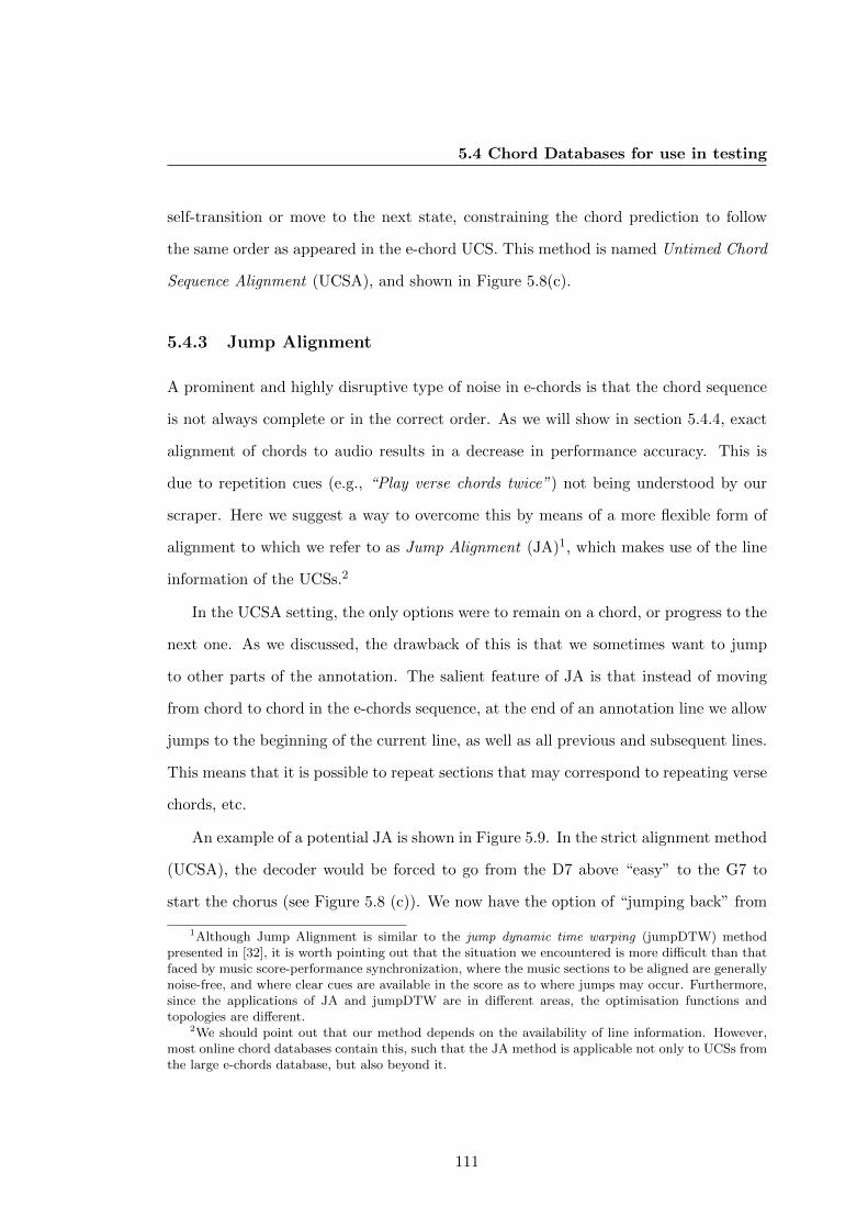
5.4 Chord Databases for use in testing
self-transition or move to the next state, constraining the chord prediction to follow
the same order as appeared in the e-chord UCS. This method is named Untimed Chord
Sequence Alignment (UCSA), and shown in Figure 5.8(c).
5.4.3 Jump Alignment
A prominent and highly disruptive type of noise in e-chords is that the chord sequence
is not always complete or in the correct order. As we will show in section 5.4.4, exact
alignment of chords to audio results in a decrease in performance accuracy. This is
due to repetition cues (e.g., “Play verse chords twice”) not being understood by our
scraper. Here we suggest a way to overcome this by means of a more flexible form of
alignment to which we refer to as Jump Alignment (JA)1, which makes use of the line
information of the UCSs.2
In the UCSA setting, the only options were to remain on a chord, or progress to the
next one. As we discussed, the drawback of this is that we sometimes want to jump
to other parts of the annotation. The salient feature of JA is that instead of moving
from chord to chord in the e-chords sequence, at the end of an annotation line we allow
jumps to the beginning of the current line, as well as all previous and subsequent lines.
This means that it is possible to repeat sections that may correspond to repeating verse
chords, etc.
An example of a potential JA is shown in Figure 5.9. In the strict alignment method
(UCSA), the decoder would be forced to go from the D7 above “easy” to the G7 to
start the chorus (see Figure 5.8 (c)). We now have the option of “jumping back” from
1Although Jump Alignment is similar to the jump dynamic time warping (jumpDTW) methodpresented in [32], it is worth pointing out that the situation we encountered is more difficult than thatfaced by music score-performance synchronization, where the music sections to be aligned are generallynoise-free, and where clear cues are available in the score as to where jumps may occur. Furthermore,since the applications of JA and jumpDTW are in different areas, the optimisation functions andtopologies are different.
2We should point out that our method depends on the availability of line information. However,most online chord databases contain this, such that the JA method is applicable not only to UCSs fromthe large e-chords database, but also beyond it.
111

5. EXPLOITING ADDITIONAL DATA
Love, Love, Love
Love, Love, Love
Love, Love, Love
There’s nothing you can do that can’t be done
There’s nothing you can sing that can’t be sung
Nothing you can say but you can learn to play the game
It’s easy
There’s nothing you can make than can’t be made
No one you can save that can’t be saved
Nothing you can do but you can learn to be you in time
It’s easy
Chorus:
All you need is love
G D7/A Em
G D7/A Em
D7/A G D7/A
G D7/F# Em
G D7/F# Em
D7/A G D/F# D7
D7/A D
G A7sus D7
1
2
Figure 5.9: Example application of Jump Alignment for the song presented in Figure 5.7.By allowing jumps from ends of lines to previous and future lines, we allow an alignmentthat follows the solid path, then jumps back to the beginning of the song to repeat theverse chords before continuing to the chorus.
112

5.4 Chord Databases for use in testing
the D7 to the beginning of the first line (or any other line). We can therefore take the
solid line path, then jump back (dashed path 1), repeat the solid line path, and then
jump to the chorus (dashed path 2). This gives us a path through the chord sequence
that is better aligned to the global structure of the audio.
This flexibility is implemented by allowing transitions corresponding to jumps back-
ward (green arrows in Figure 5.8 (d)) and jumps forward (blue arrows in Figure 5.8
(d)). The transition probability distribution P ′tr (still on the new augmented state
space A′ = {1, . . . , |e|} introduced in section 5.4.2) is then expressed as,
P ′tr(j|i,Θ, e) =
1ZPtr(ei, ej) if j ∈ {i, i+ 1}pfZ Ptr(ei, ej) if i+ 1 < j & i is the end and j the beginning of a line
pbZ Ptr(ei, ej) if i > j & i is the end and j the beginning of a line
0 otherwise.
,
(5.6)
Hence, if the current chord to be aligned is not the end of an annotation line,
the only transitions allowed are to itself or the next chord, which executes the same
operations as in UCSA. At the end of a line, an additional choice to jump backward
or forward to the beginning of any line is permitted with a certain probability. In
effect, Jump Alignment can be regarded as a constrained Viterbi alignment, in which
the length of the Viterbi path is fixed to be |X|.
This extra flexibility comes at a cost: we must specify a jump backward probability
pb and a jump forward probability pf to constrain the jumps. To tune these parameters,
we used maximum likelihood estimation, which exhaustively searches a pre-defined
(pb, pf ) matrix and picks up the pair that generates the most probable chord labelling
for an input X (note that UCSA is a special case of JA that is obtained by setting both
jump probabilities (pb, pf ) to 0).
The pseudo-code of the JA algorithm is presented in Table 5.4, where two addi-
tional matrices Pobs = {Pobs(xt|ai,Θ)|t = 1, . . . , |X| and i = 1, . . . , |A|} and P′tr =
113

5. EXPLOITING ADDITIONAL DATA
{P ′tr(j|i,Θ, e)|i, j = 1, . . . , |e|}, are introduced for notational convenience.
Table 5.4: Pseudocode for the Jump Alignment algorithm.
Input: A chromagram X and its UCS e, the observation probability matrixPobs, the transition probability matrix Ptr, the initial distribution vectorPini and the jump probabilities pb and pf
1) Restructure the transition probabilities
Initialise a new transition matrix P′tr ∈ R|e|×|e|for i = 1, . . . , |e|
for j = 1, . . . , |e|if i = j then P′tr(i, j) = Ptr(ei, ei)if i = j − 1 then P′tr(i, j) = Ptr(ei, ej)if i is the end of a line and j is the beginning of a line
if i > j then P′tr(i, j) = pb ×Ptr(ei, ej)if i < j then P′tr(i, j) = pf ×Ptr(ei, ej)
else P′tr(i, j)=0Re-normalise P′tr such that each row sums to 1
2) Fill in the travel grid
Initialise a travel grid G ∈ R|X|×|e|
Initialise a path tracing grid TR ∈ R|X|×|e|for j = 1, . . . , |e|
G(1, j) = Pobs(x1, ej)× Pini(ej)for t = 2, . . . , |X|
for j = 1, . . . , |e|G(t, j) = Pobs(xt, ej)×
|e|maxi=1
(G(t− 1, i)×P′tr(i, j))
TR(t, j) = arg|e|
maxi=1
(G(t− 1, i)×P′tr(i, j))
3) Derive the Viterbi pathThe path probability P = G(|X|, |e|)The Viterbi path V P =
{|e|}
for t = |X|, . . . , 2V P =
{TR(t, V P (1)), V P
}V P = e(V P )
Output: The Viterbi path V P and the path likelihood P
Choosing the Best Key and Redundancy
In all the above methods we needed a way of predicting which key transposition and re-
dundancy was the best to use, since there were multiple versions and key transpositions
in the database. Similar to the authors of [57], we suggest to use the log-likelihood as
a measure of the quality of the prediction (we refer to this scheme as “Likelihood”).
114

5.4 Chord Databases for use in testing
In the experiments in section 5.4.4 we investigate the performance of this approach
to estimate the correct transposition, showing that it is almost as accurate as using the
key and transposition that maximised the performance (which we call “Accuracy”).
5.4.4 Experiments
In order to evaluate the performance of using online chord databases in testing, we
must test on songs for which the ground truth is currently available. Being the most
prominent single artist in any of our datasets, we chose The Beatles as our test set.
We used the USpop dataset to train the parameters for an HMM and used these, in
addition with increasing amounts of online information, to decode the chord sequence
for each of the songs in the test set.
We found that 174 of the 180 songs had at least one file on e-chords.com, and we
therefore used this as our test set. Although a full range of complex chords are present
in the UCSs, we choose to work with the minmaj alphabet as a proof of concept.
We used either the true chord sequence (GTUCS), devoid of timing information, or the
genuine UCS; and chose the best key and redundancy using either the largest likelihood
or best performance. Results are shown in Table 5.5. From a baseline prediction level
Table 5.5: Results using online chord annotations in testing. Amount of informationincreases left to right, Note Precision is shown in the first 3 rows. p–values using theWilcoxon signed rank test for each result with respect to that to the left of it are shownin rows 4–6.
Model
HMM ACV ATCV UCSA JA
NP (%)GTUCS 76.33 80.40 83.54 88.76 −Accuracy 76.33 79.56 81.19 73.10 83.64Likelihood 76.33 79.02 80.95 72.61 82.12
p-valueGTUCS − 2.73e− 28 1.06e− 23 1.28e− 29 −Accuracy − 7.07e− 12 5.52e− 11 4.13e− 14 4.67e− 9Likelihood − 1.63e− 15 2.3e− 10 3.05e− 13 7.19e− 27
115
5. EXPLOITING ADDITIONAL DATA
of 76.33% Note Precision, we see a rapid improvement in recognition rates by using
the ground truth UCS (top row of Table 5.5, peaking at 88.76%). Note that JA is
neither possible nor necessary with the ground truths, as we know that the chords in
the Ground Truth are in the correct order.
When using genuine UCSs, we also see an improvement when using Alphabet Con-
strained Viterbi (ACV, column 2) and Alphabet and Transition Constrained Viterbi
(ATCV, column 3). However, when attempting to align the UCSs to the chromagram
(UCSA, column 4), performance decreases. Upon inspection of the decoded sequences,
we discovered that this was because complex line information (Play these chords twice,
etc.) were not understood by our scraper. To counteract this, we employed Jump Align-
ment (JA, final column) where we saw an increase in recognition rate, although the
recognition rate naturally does not match performance when using the true sequence.
Comparing the likelihood method to the accuracy (rows 2 to 3), we see that both
models are very competitive, suggesting that using the likelihood is often picking the
correct key and most useful redundancy of a UCS. Inspecting the p–values (rows 4–
6) shows that all increases in performances are statistically significant at the 1% level.
This is a significant result, as it shows that knowledge of the correct key and most infor-
mative redundancy offers only a slight improvement over the fully automatic approach.
However, statistical tests were also conducted to ascertain whether the difference be-
tween the Accuracy and Likelihood settings of Table 5.5 were significant on models
involving the use of UCSs. Wlicoxon signed rank tests yielded p-values of less than
0.05 in all cases, suggesting that true knowledge of the ‘best’ key and transposition
offers significant benefits when exploiting UCSs in ACE. We show the data from Table
5.5 in Figure 5.10, where the benefit of using additional information from internet chord
annotations and the similarity between the “likelihood” and “accuracy” schemes are
easily seen.
116
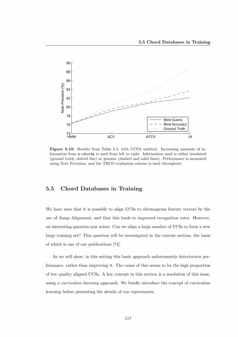
5.5 Chord Databases in Training
HMM ACV ATCV JA74
76
78
80
82
84
86
88
90N
ote
Pre
cisi
on (
%)
Best Guess Best Accuracy Ground Truth
Figure 5.10: Results from Table 5.5, with UCSA omitted. Increasing amounts of in-formation from e-chords is used from left to right. Information used is either simulated(ground truth, dotted line) or genuine (dashed and solid lines). Performance is measuredusing Note Precision, and the TRCO evaluation scheme is used throughout.
5.5 Chord Databases in Training
We have seen that it is possible to align UCSs to chromagram feature vectors by the
use of Jump Alignment, and that this leads to improved recognition rates. However,
an interesting question now arises: Can we align a large number of UCSs to form a new
large training set? This question will be investigated in the current section, the basis
of which is one of our publications [74].
As we will show, in this setting this basic approach unfortunately deteriorates per-
formance, rather than improving it. The cause of this seems to be the high proportion
of low quality aligned UCSs. A key concept in this section is a resolution of this issue,
using a curriculum learning approach. We briefly introduce the concept of curriculum
learning before presenting the details of our experiments.
117
5. EXPLOITING ADDITIONAL DATA
5.5.1 Curriculum Learning
It has been shown that humans and animals learn more efficiently when training exam-
ples are presented in a meaningful way, rather than in a homogeneous manner [28, 50].
Exploiting this feature of learners is referred to as Shaping, in the animal training
community, and Curriculum Learning (CL), in the machine learning discipline [6].
The core assumption of the CL paradigm is that starting with easy examples and
slowly generalising leads to more efficient learning. In a machine learning setting this
can be realised by carefully selecting training data from a large set of examples. In
[6], the authors hypothesize that CL offers faster training (both in optimization and
statistical terms) in online training settings, owing to the fact that the learner wastes
less time with noisy or harder–to–predict examples. Additionally, the authors assume
that guiding the training into a desirable parameter space leads to better generalization.
Due to high variability in the quality of e–chords UCSs, CL seems a particularly
promising idea to help us make use of aligned UCSs in an appropriate preference order,
from easy to difficult. Until now we have not defined what we understand by “easy”
examples or how to sort the available examples in order of increasing difficulty. The
CL paradigm provides little formal guidance for how to do this, but generally speaking,
easy examples are those that the recognition system can already handle fairly well, such
that considering them will only incrementally alter the recognition system.
Thus, we need a way to quantify how well our chord recognition system is able to
annotate chords to audio for which we only have UCSs and no ground truth annotations.
To this end, we propose a new metric for evaluating chord sequences based on a UCS
only. We will refer to this metric as the Alignment Quality Measure.
In summary, our CL approach rests on two hypotheses:
1. Introducing “easy” examples into the training set leads to faster learning.
2. The Alignment Quality Measure quantifies how “easy” a song with associated
118

5.5 Chord Databases in Training
UCS is for the current chord recognition system, more specifically whether it is
able to accurately annotate the song with chords.
Both these hypotheses are non–trivial, and we will empirically confirm their validity
below.
5.5.2 Alignment Quality Measure
We first address the issue of determining the quality of UCS alignment without the aid
of ground truth. In our previous work [73], we used the likelihood of the alignment
(normalised by the number of frames) as a proxy for the alignment quality. In this
work we take a slightly different approach, which we have found to be more robust.
Let {AUCS}Nn=1 be a set of UCSs aligned using Jump Alignment. For each UCS
chromagram, we made a simple HMM prediction using the core training set to create
a set of predictions {HMM}Nn=1. We then compared these predictions to the aligned
UCS to estimate how close the alignment has come to a rough estimate of the chords.
Thus, we define:
γi =1
|AUCSi|
|AUCSi|∑t=1
I(AUCSti = HMMt
i) (5.7)
where I is an indicator function and AUCSti and HMMt
i represent the tth frame of the
ith aligned UCS and HMM prediction, respectively.
We tested the ability of this metric to rank the quality of the alignments, using
the set–up from the experiments in subsection 5.4.4 (ground truths were required to
test this method). We found the rank correlation between γ and the actual HMM
performance to be 0.74, with a highly significant p–value of p < 10−30, indicating that
point 2 has been answered (i.e., we have an automatic method of measuring how good
the alignment of a UCS to a chromagram is).
119
5. EXPLOITING ADDITIONAL DATA
5.5.3 Results and Discussion
Confident that we now have a method for assessing alignment quality, we set about
aligning a large number of UCSs to form a new training set. We took the MIREX
dataset as the core training set, and trained an HMM on these data. These parameters
were then used to align 1, 683 UCSs for which we had audio (we only used UCSs that had
at least 10 chord symbols to clean the data, reducing the dataset from 1, 822 examples).
We then ran an HMM over these chroma and calculated the alignment quality γ for
each of the aligned UCSs. These were then sorted and added in descending order to
the core training set. Finally, an HMM was re–trained on the union of the core and
expansion sets and tested on the union of the USpop and Billboard datasets.
From our previous work [73], we know that expanding the training set is only
beneficial when the task is sufficiently challenging (a system that already performs well
has little need of additional training data). For this reason, we evaluated this task on
the MM alphabet. Results are shown in Figure 5.11.
Here we show the alignment quality threshold on the x–axis, with the number
of UCSs this corresponds to on the left y–axis. The baseline performance occurs at
alignment quality threshold ∞, i.e., when we use no UCSs and the threshold is shown
as a grey, dashed line; whilst performance using the additional UCSs is shown as a
solid black line, with performance being measured in both cases in TRCO on the right
y–axis.
The first observation is that there are a large number of poor–quality aligned UCSs,
as shown by the large number of expansion songs in the left–most bin for number of
expansion songs. Including all of these sequences leads to a large drop in performance,
from a baseline of 52.34% to 47.50% TRCO Note Precision. Fortunately, we can auto-
matically remove these poor–quality aligned UCSs via the alignment quality measure
γ. By being more stringent with our data (γ → 1), we see that, although the number of
additional training examples drops, we begin to see a boost in performance, peaking at
120
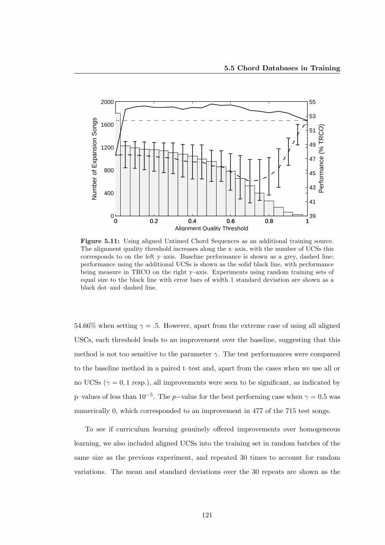
5.5 Chord Databases in Training
0 0.2 0.4 0.6 0.8 10
400
800
1200
1600
2000N
umbe
r of
Exp
ansi
on S
ongs
0 0.2 0.4 0.6 0.8 139
41
43
45
47
49
51
53
55
Alignment Quality Threshold
Per
form
ance
(%
TR
CO
)
Figure 5.11: Using aligned Untimed Chord Sequences as an additional training source.The alignment quality threshold increases along the x–axis, with the number of UCSs thiscorresponds to on the left y–axis. Baseline performance is shown as a grey, dashed line;performance using the additional UCSs is shown as the solid black line, with performancebeing measure in TRCO on the right y–axis. Experiments using random training sets ofequal size to the black line with error bars of width 1 standard deviation are shown as ablack dot–and–dashed line.
54.66% when setting γ = .5. However, apart from the extreme case of using all aligned
USCs, each threshold leads to an improvement over the baseline, suggesting that this
method is not too sensitive to the parameter γ. The test performances were compared
to the baseline method in a paired t–test and, apart from the cases when we use all or
no UCSs (γ = 0, 1 resp.), all improvements were seen to be significant, as indicated by
p–values of less than 10−5. The p−value for the best performing case when γ = 0.5 was
numerically 0, which corresponded to an improvement in 477 of the 715 test songs.
To see if curriculum learning genuinely offered improvements over homogeneous
learning, we also included aligned UCSs into the training set in random batches of the
same size as the previous experiment, and repeated 30 times to account for random
variations. The mean and standard deviations over the 30 repeats are shown as the
121
5. EXPLOITING ADDITIONAL DATA
dot–and–dashed line and bars in Figure 5.11. We can see that the specific ordering of
the expansion set offers substantial improvement over randomly selecting the expansion
set, and in fact, ordering the data randomly never reaches the baseline performance.
This is good evidence that curriculum learning is the method of choice for navigating a
large set of training examples, and also demonstrates that the first assumption of the
Curriculum Learning paradigm holds.
5.6 Conclusions
This chapter was concerned with retraining our model on datasets outside the MIREX
paradigm. We saw that training a model on a small amount of data can lead to
strong overfitting and poor generalisation (for instance, training on seven Carole King
tracks). However, when sufficient training data exists we attain good training and
test performances, and noted in particular that generalisation between the Billboard,
MIREX and USpop datasets is good. Across more complex chord alphabets, we see a
drop in performance as the complexity of chords increases, as is to be expected.
We also showed the dominance of HPA over the baseline HMM on all datasets that
contained key information on which to train. Using leave–one–out testing, we saw that
an overall estimate of the test set performance was 54.73%−70.71% TRCO, depending
on the alphabet used, although the variance in this setting is large. Following this,
we investigated how fast HPA learns by constructing learning curves, and found that
the initial learning rate is fast, but appears to plateau for simpler alphabets such as
minmaj.
The next main section of this chapter looked at online chord databases as an ad-
ditional source of information. We first investigated if chord sequences obtained from
the web could be used in a test setting. Specifically, we constrained the output of the
Viterbi decoder according to these sequences to see if they could aid decoding perfor-
122

5.6 Conclusions
mance. We experienced an increase in recognition performance from 76.33% to 79.02%
by constraining the alphabet, and 80.95% by constraining the alphabet and transitions,
but a drop to 72.61% when aligning the sequences to the audio. However, this drop
was resolved by the use of Jump Alignment, where we attained 82.12% accuracy. All
of the results above were obtained by choosing the key and redundancy for a UCS
automatically.
Next, we investigated whether aligning a large number of UCSs to audio could form
a new training set. By training on the MIREX dataset, we aligned a large number
of UCSs to chromagram feature vectors and experienced an increase of 2.5 percentage
points when using a complex chord alphabet. This was obtained by using an alignment
quality measure γ to estimate how successful an alignment of a UCS to audio was. These
were then sorted and added to the data in decreasing order, in a form of curriculum
learning. Performance peaked when using γ = 0.5, although using any number of
sequences apart from the worst ones led to an improvement. We also experimentally
verified that the curriculum learning setting is essential if we are to use UCSs as a
training source by adding aligned UCSs to the expansion set in random order.
123
5. EXPLOITING ADDITIONAL DATA
124
6
Conclusions
In this thesis, we have designed and tested a new method for the extraction of musical
chords from audio. To achieve this, we conducted a review of the literature in the field,
including the annual benchmarking MIREX evaluations. We also defined a new feature
for use in chord recognition, the loudness-based chromagram. Decoding was achieved by
Viterbi inference using our Dynamic Bayesian Network HPA (the Harmony Progression
Analyser); we achieved cutting-edge performance when deploying this method on the
MIREX dataset. We also saw that HPA may be re-trained on new ground truth data
as it arises, and tested this on several new datasets.
In this brief chapter, we review the main findings and results in section 6.1 and
suggest areas for further research in section 6.2.
6.1 Summary
Chapter 1: Introduction
In the opening chapter, we first defined the task of automatic chord estimation as the
unaided extraction of chord labels and boundaries from audio. We then motivated our
work as a combination of three factors: the desire to make a tool for amateur musi-
125

6. CONCLUSIONS
cians for educational purposes, the use of chord sequences in higher-level MIR tasks,
and the promise that recent machine-learning techniques have shown in tasks such as
image recognition and automatic translation. Next, we outlined our research objectives
and contributions, with reference to the thesis structure and main publications by the
author.
Chapter 2: Background
In chapter 2, we looked at chords and their musical function. We defined a chord
as occurring when three or more notes are sounded simultaneously, or functioning as
if sounded simultaneously [93]. This led into a discussion of musical keys, and we
commented that it is sometimes more convenient to think of a group of chords as
defining a key - sometimes conversely. Several authors have exploited this fact by
estimating chords and keys simultaneously [16, 57].
We next gave a chronological account of the literature for the domain of Automatic
Chord Estimation. We found that through early work on Pitch Class Profiles, Fu-
jishima [33] was able to estimate the chords played on a solo piano by using pattern
matching techniques in real time. A breakthrough in feature extraction came in 2001
when [79] used a constant-Q spectrum to characterise the energy of the pitch classes
in a chromagram. Since then, other techniques for improving the accuracy of chord
recognition systems have included the removal of background spectra and/or harmon-
ics [65, 96, 111], compensation for tuning [38, 44, 99], smoothing/beat synchronisation
[4, 52], mapping to the tonal centroid space [37], and integrating bass information
[63, 107].
We saw that the two dominant models in the literature are template-based methods
[15, 86, 106] and Hidden Markov Models [19, 87, 99]. Some authors have also explored
using more complex models, such as HMMs, with an additional chain for the musical
key [100, 119] or larger Dynamic Bayesian Networks [65]. In addition to this, some
126
6.1 Summary
research has explored whether a language model is appropriate for modelling chords
[98, 117], or if discriminative modelling [12, 115] or genre-specific models [55] offer
superior performance.
With regard to evaluation, the number of correctly identified frames divided by the
total number of frames is the standard way of measuring performance for a song, with
Total Relative Correct Overlap and Average Relative Correct Overlap being the most
common evaluation schemes when dealing with many songs. Most authors in the field
reduce their ground truth and predicted chord labels to major and minor chords only
[54, 87], although the main triads [12, 118] and larger alphabets [65, 99] have also been
considered.
Finally, we conducted a review in this chapter of the Music Information Evalu-
ation eXchange (MIREX), which has been benchmarking ACE systems since 2008.
Significantly, we noted that the expected trend of pre-trained systems outperforming
train/test systems was not observed every year. This, however, was highlighted by
our own submission NMSD2 in 2011, which attained 97.60 TRCO, underscoring the
difficulty in using MIREX as a benchmarking system when the test data is known.
Chapter 3: Chromagram Extraction
In this chapter, we first discussed our motivation for calculating loudness-based chro-
magram feature vectors. We then detailed the preprocessing that an audio waveform
undergoes before analysis. Specifically, we downsample to 11, 025 samples per second,
collapse to mono, and employ Harmonic and Percussive Sound Separation to the wave-
form. We then estimate the tuning of the piece using an existing algorithm [26] to
modify the frequencies we search for in the calculation of a constant-Q based spec-
trogram. The loudness at each frequency is then calculated and adjusted for human
sensitivity by the industry-standard A-weighting [103] before octave summing, beat-
synchronising and normalising our features.
127
6. CONCLUSIONS
Experimentally, we first described how we attained beat-synchronised ground truth
annotations to match our features. We then tested each aspect of our feature extrac-
tion process on the MIREX dataset of 217 songs, and found that the best performance
(80.91% TRCO) was attained by using the full complement of signal processing tech-
niques.
Chapter 4: Dynamic Bayesian Network
A mathematical description of our Dynamic Bayesian Network (DBN), the Harmony
Progression Analyser (HPA), was the first objective of this chapter. This DBN has
hidden nodes for chords, bass notes, and key sequences and observed nodes representing
the treble and bass frequencies of a musical piece. We noted that this number of nodes
and links places enormous constraints on the decoding and memory costs of HPA, but
we showed that two-stage predictions and making use of the training data permitted
us to reduce the search space to an acceptable level.
Experimentally, we then built up the nodes used in HPA from a basic HMM. We
found that the full HPA model performed the best in a train/test setting, achieving
83.52% TRCO in an experiment comparable to the MIREX competition, and attaining
a result equal to the current state of the art. We also introduced two metrics for
evaluating ACE systems: chord precision (which measures 1 if the chord symbols in
ground truth and prediction are identical), and note precision (1 if the notes in the
chords are the same, 0 otherwise). We noted that the key accuracies for our model
were quite poor. Bass accuracies on the other hand were high, peaking at 86.08%.
Once the experiments on major and minor chords were complete (Section 4.2),
we moved on to larger chord alphabets, including all triads and some chords with 4
notes, such as 7ths. We found that chord accuracies generally decreased, which was
as expected, but that results were at worst 57.76% (chord precision, Quads alphabet,
c.f. Minmaj at 74.08%). Specifically, performance for the triads alphabet peaked
128
6.1 Summary
at 78.85% Note Precision TRCO, whilst the results for the MM and Quads alphabets
peaked at 66.53% and 66.50%, respectively. Not much change was seen across alphabets
when using the MIREX metric, which means that this method is not appropriate for
evaluating complex chord alphabets. We also saw that HPA significantly outperformed
an HMM in all tasks described in this chapter, and attained performance in line with
the current state of the art (82.45% TRCO c.f. KO1 submission in 2011, 82.85%).
Chapter 5: Exploiting Additional Data
In chapter 5, we tested HPA on a variety of ground truth datasets that have recently
become available. These included the USpop set of 194 ground truth annotations, and
Billboard set of 522 songs, as well as two small sets by Carole King (7 songs) and Oasis
(5 songs). We saw poor performances when training on the small datasets of Carole
King and Oasis, which highlights a disadvantage of using data-driven systems such as
HPA.
However, when training data is sufficient, we attain good performances on all
chord alphabets. Particularly interesting was that training and testing on the Bill-
board/MIREX datasets gave performances similar to using HPA (train Billboard, Test
MIREX = 76.56% CP TRCO, train MIREX, test Billboard = 69.06% CP TRCO in
the minmaj alphabet), although the difficulty of testing on varied artists is highlighted
by the poorer performance when testing on Billboard. This does, however, show that
HPA is able to transfer learning from one dataset to another, and gives us hope that it
has good potential for generalisation.
Through leave-one-out testing, we were able to generate a good estimate of how
HPA deals with a mixed-test set of the MIREX, Billboard and Carole King datasets.
Performances here were slightly lower than in earlier experiments, and the variance was
high, again underscoring the difficulty of testing on a diverse set. We also investigated
how quickly HPA learns. Through plotting learning curves, we found out that HPA is
129
6. CONCLUSIONS
able to attain good performances on the Billboard, and that learning is fastest when
the task is most challenging (MM and Quads alphabets).
We then went on to see how Untimed Chord Sequences (UCSs) can be used to
enhance prediction accuracy for songs, when available. This was conducted by using
increasing amounts of information from UCSs from e-chords.com, where we found that
prediction accuracy increased from a baseline of 76.33% NP to 79.02% and 80.95% by
constraining the alphabet, and then transitions, allowed in the Viterbi inference. When
we tried to align the UCSs to the audio, we experienced a drop in performance to
72.61%, which we attributed to our assumption that the chord symbols on the website
are in the correct order, with no jumping through the annotation required. However,
this problem was overcome by the use of the Jump Alignment algorithm, which was
able to resolve these issues and attained performance of 82.12%.
In addition to their use in a test setting, we also discovered that aligned UCSs may
be used in a training scenario. Motivated by the steep learning curves for complex
chord alphabets seen in 5.3 and our previous results [73], we set about aligning a set of
1, 683 UCSs to audio, using the MIREX dataset as a core training set. We then trained
an HMM on the core training set, as well as the union of the core and expansion set,
and tested on the USpop and Billboard datasets, where we experienced an increase in
recognition rate from 52.34% to 54.66% TRCO. This was attained by sorting the aligned
UCSs according to alignment quality, and adding to the expansion set incrementally,
beginning with the “easiest” examples first in a form of curriculum learning, that was
shown to lead to an improvement in learning as opposed to homogeneous training.
6.2 Future Work
Through the course of this thesis, we have come across numerous situations where
further investigation would be interesting or insightful. We present a summary of these
130

6.2 Future Work
concepts here.
Publication of Literature Summary
In the review of the field that we conducted in section 2.2, we collated many of the
main research papers conducted on automatic chord estimation, and also summarised
the results of the MIREX evaluations from the past four years. We feel that such work
could be of use to the research community as an overview or introduction to the field,
and hence worthy of publication.
Local Tuning
The tuning algorithm we used [26] estimates global tuning by peak selecting in the
histogram of frequencies found in a piece. However, it is possible that the tuning
may change within one song, and that a local tuning method may yield more accurate
chromagram features. “Strawberry Fields Forever” (Lennon/McCartney) is an example
of one such song, where the CD recording is a concatenation of two sessions, each with
slightly different pitch.
Investigation of Key Accuracies
In section 4.2.3, we found that the key accuracy of HPA was quite poor in comparison
to the results attained when recognising chords. It seems that we were either correctly
identifying the correct key for all frames, or completely wrong (see Figures 4.2a, 4.2b,
4.2c). The reason for this could be an inappropriate model or an issue of evaluation.
For example, an error in predicting the key of G Major instead of C Major is a distance
of 1 around the cycle of fifths and is not as severe as confusing C Major with F] Major.
This is not currently factored into the frame-wise performance metric employed in this
work (nor is it for evaluation of chords).
131

6. CONCLUSIONS
Evaluation Strategies
We introduced two metrics for ACE in this thesis (Note Precision and Chord Preci-
sion) to add to the MIREX-style evaluation. However, each of these outputs a binary
correct/incorrect label for each frame, whereas a more flexible approach is more likely
to give insight into the kinds of errors ACE systems are making.
Intelligent Training
In subsection 5.1.2, we saw that HPA is able to learn from one dataset (i.e., MIREX) and
test on another (USpop), yielding good performance when training data is sufficient.
However, within this section and throughout this thesis, we have assumed that the
training and testing data come from the same distribution, whereas this may not be
the case in reality.
One way of dealing with this problem would be to use transfer learning [82] to share
information (model parameters) between tasks, which has been used in the past on a
series of related tasks in medical diagnostics and car insurance risk analysis. We believe
that this paradigm could lead to greater generalisation than the training scheme offered
within this thesis.
Another approach would be to use a genre-specific model, as proposed by Lee [55].
Although genre tags are not readily available for all of our datasets, information could
be gathered from several sources, including last.fm1, the echonest2 or e-chords3. This
information could be used to learn one model per genre in training, with all genre
models being used for testing, and a probabilistic method being used to assign the
most likely genre/model to a test song.
1www.last.fm2the.echonest.com3www.e-chords.com
132
6.2 Future Work
Key Annotations for the USpop data
It is unfortunate that we could not train HPA on the USpop dataset, owing to the lack
of key annotations. Given that this is a relatively small dataset, a fruitful area of future
work would be to hand-annotate these data.
Improving UCS to chromagram pairings
When we wish to obtain the UCS for a given song (defined as an artist/title pair), we
need to query the database of artists and song titles from our data source to see how
many, if any, UCSs are available for this song. Currently, this is obtained by computing
a string equality between the artist and song title in the online database and our audio.
However, this method neglects errors in spelling, punctuation, and abbreviations, which
are rife in our online source (consider the number of possible spellings and abbreviations
of “Sgt. Pepper’s Lonely Hearts Club Band”).
This pairing could be improved by using techniques from the named entity recogni-
tion literature [108], perhaps in conjunction with some domain specific heuristics such
as stripping of “DJ” (Disk Jockey) or “MC” (Master of Ceremonies). An alternative
approach would be to make use of services from the echonest or musicbrainz1, who spe-
cialise in such tasks. Improvements in this area will undoubtedly lead to more UCSs
being available, and yield higher gains when these data are used in a testing setting via
Jump Alignment.
Improvements in Curriculum Learning
We saw in section 5.5.1 that a curriculum learning paradigm was necessary to see
improvements when using UCSs as an additional training source. The specification of
the alignment quality measure γ was noticed to show improvements for γ ≥ 0.15, but
1musicbrainz.org/
133

6. CONCLUSIONS
a more thorough investigation of the sensitivity of this parameter and how it may be
set may lead to further improvements in this setting.
Creation of an Aligned Chord Database
As an additional resource to researchers, it would be beneficial to release a large number
of aligned UCSs to the community. Although we know that these data must be used
with care, releasing such a database would still be a valuable tool to researchers and
would constitute by far the largest and most varied database of chord annotations
available.
Applications to Higher-level tasks
We mentioned in the introduction that applications to higher-level tasks was one mo-
tivation for this work. Given that we now have a cutting-edge system, we may begin
to think about possible application areas in the field of MIR. Previously, for example,
the author has worked on mood detection [71] and hit song science [80], where pre-
dicted chord sequences could be used as features for identifying melancholy or tense
songs (large number of minor/diminished chords) or successful harmonic progressions
(popular chord n−grams)
134
References
[1] Techniques for note identification in polyphonic music. CCRMA, Department of
Music, Stanford University, 1985.
[2] M. Barthet, A. Anglade, G. Fazekas, S. Kolozali, and R. Macrae. Music recom-
mendation for music learning: Hotttabs, a multimedia guitar tutor. Workshop on
Music Recommendation and Discory, collated with ACM RecSys 2011 Chicago,
IL, USA October 23, 2011, page 7, 2011.
[3] M.A. Bartsch and G.H. Wakefield. To catch a chorus: Using chroma-based repre-
sentations for audio thumbnailing. In Applications of Signal Processing to Audio
and Acoustics, 2001 IEEE Workshop on the, pages 15–18. IEEE, 2001.
[4] J.P. Bello and J. Pickens. A robust mid-level representation for harmonic con-
tent in music signals. In Proceedings of the 6th International Society for Music
Information Retrieval (ISMIR), pages 304–311, 2005.
[5] J.P. Bello, G. Monti, and M. Sandler. Techniques for automatic music transcrip-
tion. In International Symposium on Music Information Retrieval, pages 23–25,
2000.
[6] Y. Bengio, J. Louradour, R. Collobert, and J. Weston. Curriculum learning.
In Proceedings of International Conference on Machine Learning, pages 41–48.
ACM, 2009.
135
REFERENCES
[7] A. Berenzweig, B. Logan, D.P.W. Ellis, and B. Whitman. A large-scale evaluation
of acoustic and subjective music-similarity measures. Computer Music Journal,
28(2):63–76, 2004.
[8] R. Bisiani. Beam search. Encyclopedia of Artificial Intelligence, 2, 1987.
[9] E.O. Brigham and R.E. Morrow. The fast Fourier transform. Spectrum, IEEE,
4(12):63–70, 1967.
[10] J. Brown. Calculation of a constant q spectral transform. Journal of the Acoustical
Society of America, 89(1):425–434, 1991.
[11] J.A. Burgoyne and L.K. Saul. Learning harmonic relationships in digital audio
with Dirichlet-based hidden Markov models. In Proceedings of the International
Conference on Music Information Retrieval (ISMIR), pages 438–443, 2005.
[12] J.A. Burgoyne, L. Pugin, C. Kereliuk, and I. Fujinaga. A cross-validated study of
modelling strategies for automatic chord recognition in audio. In Proceedings of
the 8th International Conference on Music Information Retrieval, pages 251–254,
2007.
[13] J.A. Burgoyne, J. Wild, and I. Fujinaga. An expert ground truth set for audio
chord recognition and music analysis. In Proceedings of the 12th International
Society for Music Information Retrieval (ISMIR), pages 633–638, 2011.
[14] E.M. Burns and W.D. Ward. Intervals, scales, and tuning. The psychology of
music, 2:215–264, 1999.
[15] G. Cabral, F. Pachet, and J.P. Briot. Automatic x traditional descriptor ex-
traction: The case of chord recognition. In Proceedings of the 6th international
conference on music information retrieval, pages 444–449, 2005.
136
REFERENCES
[16] B. Catteau, J.P. Martens, and M. Leman. A probabilistic framework for audio-
based tonal key and chord recognition. Advances in Data Analysis, pages 637–644,
2007.
[17] C. Chafe and D. Jaffe. Source separation and note identification in polyphonic
music. In Acoustics, Speech, and Signal Processing, IEEE International Confer-
ence on, volume 11, pages 1289–1292. IEEE, 1986.
[18] E. Chew. Towards a mathematical model of tonality. PhD thesis, Massachusetts
Institute of Technology, 2000.
[19] T. Cho and J.P. Bello. Real-time implementation of HMM-based chord estimation
in musical audio. In Proceedings of the International Computer Music Conference
(ICMC), pages 16–21, 2009.
[20] T. Cho and J.P. Bello. A feature smoothing method for chord recognition us-
ing recurrence plots. In Proceedings of the 12th International Society for Music
Information Retrieval Conference (ISMIR), 2011.
[21] T. Cho, R.J. Weiss, and J.P. Bello. Exploring common variations in state of the
art chord recognition systems. In Proceedings of the Sound and Music Computing
Conferecne (SMC), 2010.
[22] D. Conklin and I.H. Witten. Prediction and entropy of music. Master’s thesis,
Department of Computer Science, University of Calgary, 1990.
[23] D. Cope. Hidden structure: music analysis using computers, volume 23. AR
Editions, 2008.
[24] D. Deutsch. The psychology of music. Academic Press, 1999.
[25] R. Durbin, S. Eddy, A. Krogh, and G. Mitchison. Biological sequence analysis:
137

REFERENCES
probabilistic models of proteins and nucleic acids. Cambridge University Press,
1998.
[26] D. Ellis and A. Weller. The 2010 labROSA chord recognition system. Proceedings
of the 11th Society for Music Information Retrieval, Music Information Retrieval
Evaluation exchange paper), 2010.
[27] D.P.W. Ellis and G.E. Poliner. Identifying ‘cover songs’ with chroma features and
dynamic programming beat tracking. In Acoustics, Speech and Signal Processing,
IEEE International Conference on, volume 4, pages IV–1429. IEEE, 2007.
[28] J.L. Elman. Learning and development in neural networks: the importance of
starting small. Cognition, 48(1):71–99, 1993. ISSN 0010-0277.
[29] H. Fletcher. Loudness, its definition, measurement and calculation. Journal of
the Acoustical Society of America, 5(2):82, 1933.
[30] M. Florentine. It’s not recruitment-gasp!! it’s softness imperception. The Hearing
Journal, 56(3):10, 2003.
[31] D. Fogel, J.C. Hanson, R. Kick, H.A. Malki, C. Sigwart, M. Stinson, E. Turban,
and S.H. Chairman-Rubin. The impact of machine learning on expert systems.
In Proceedings of the 1993 ACM conference on Computer science, pages 522–527.
ACM, 1993.
[32] C. Fremerey, M. Muller, and M. Clausen. Handling repeats and jumps in score-
performance synchronization. In Proceedings of the 11th International Society for
Music Information Retrieval (ISMIR), pages 243–248, 2010.
[33] T. Fujishima. Realtime chord recognition of musical sound: a system using com-
mon lisp music. In Proceedings of the International Computer Music Conference,
pages 464–467, 1999.
138
REFERENCES
[34] E. Gomez and P. Herrera. The song remains the same: Identifying versions of
the same piece using tonal descriptors. In Proceedings of the 7th International
Conference on Music Information Retrieval (ISMIR), pages 180–185, 2006.
[35] M. Goto and Y. Muraoka. Real-time beat tracking for drumless audio signals:
Chord change detection for musical decisions. Speech Communication, 27(3):
311–335, 1999.
[36] C. Harte, M. Sandler, S. Abdallah, and E. Gomez. Symbolic representation of
musical chords: A proposed syntax for text annotations. In Proceedings of the 6th
International Conference on Music Information Retrieval (ISMIR), pages 66–71.
Citeseer, 2005.
[37] C. Harte, M. Sandler, and M. Gasser. Detecting harmonic change in musical
audio. In Proceedings of the 1st ACM workshop on Audio and music computing
multimedia, pages 21–26. ACM, 2006.
[38] C.A. Harte and M. Sandler. Automatic chord identification using a quantised
chromagram. In Proceedings of the Audio Engineering Society, pages 291–301,
2005.
[39] BS ISO. 226: Acoustics normal equal loudness-level contours. International
Organization for Standardization, 2003.
[40] N. Jiang, P. Grosche, V. Konz, and M. Muller. Analyzing chroma feature types
for automated chord recognition. In Proceedings of the 42nd Audio Engineering
Society Conference, 2011.
[41] N.F. Johnson. Two’s company, three is complexity: a simple guide to the science
of all sciences. Oneworld Publications Ltd, 2007.
[42] O. Karolyi. Introducing music. Penguin (Non-Classics), 1965.
139
REFERENCES
[43] K. Kashino and N. Hagita. A music scene analysis system with the MRF-based
information integration scheme. In Pattern Recognition, Proceedings of the 13th
International Conference on, volume 2, pages 725–729. IEEE, 1996.
[44] M. Khadkevich and M. Omologo. Phase-change based tuning for automatic chord
recognition. In Proceedings of Digital Audio Effects Conference (DAFx), 2009.
[45] M. Khadkevich and M. Omologo. Use of hidden Markov models and factored
language models for automatic chord recognition. In Proceedings of the Interna-
tional Society for Music Information Retrieval Conference (ISMIR), pages 561–
566, 2009.
[46] Y.E. Kim, D.S. Williamson, and S. Pilli. Towards quantifying the album effect in
artist identification. In Proceedings of the 7th International Conference on Music
Information Retrieval (ISMIR), pages 393–394, 2006.
[47] A. Klapuri and M. Davy. Signal processing methods for music transcription.
Springer-Verlag New York Inc, 2006.
[48] R. Kohavi. A study of cross-validation and bootstrap for accuracy estimation
and model selection. In International Joint Conference on Artificial Intelligence,
volume 14, pages 1137–1145, 1995.
[49] V. Konz, M. Muller, and S. Ewert. A multi-perspective evaluation framework for
chord recognition. In Proceedings of the 11th International Conference on Music
Information Retrieval (ISMIR), pages 9–14, 2010.
[50] K.A. Krueger and P. Dayan. Flexible shaping: How learning in small steps helps.
Cognition, 110(3):380–394, 2009. ISSN 0010-0277.
[51] C.L. Krumhansl. Cognitive foundations of musical pitch. Oxford University Press,
USA, 2001.
140

REFERENCES
[52] S. Kullback and R.A. Leibler. On information and sufficiency. The Annals of
Mathematical Statistics, 22(1):79–86, 1951.
[53] C.L. Lawson and R.J. Hanson. Solving least squares problems, volume 15. Society
for Industrial Mathematics, 1995.
[54] K. Lee. Automatic chord recognition from audio using enhanced pitch class pro-
file. In Proc. of the Intern. Computer Music Conference (ICMC), New Orleans,
USA, 2006.
[55] K. Lee. A system for automatic chord transcription from audio using genre-
specific hidden Markov models. Adaptive Multimedial Retrieval: Retrieval, User,
and Semantics, pages 134–146, 2008.
[56] K. Lee and M. Slaney. A unified system for chord transcription and key extraction
using hidden Markov models. In Proceedings of the 8th International Conference
on Music Information Retrieval (ISMIR), 2007.
[57] K. Lee and M. Slaney. Acoustic chord transcription and key extraction from
audio using key-dependent HMMs trained on synthesized audio. Audio, Speech,
and Language Processing, IEEE Transactions on, 16(2):291–301, 2008.
[58] F. Lerdahl. Tonal pitch space. Oxford University Press, USA, 2005.
[59] R. Macrae and S. Dixon. A guitar tablature score follower. In Multimedia and
Expo (ICME), 2010 IEEE International Conference on, pages 725–726. IEEE,
2010.
[60] R. Macrae and S. Dixon. Guitar tab mining, analysis and ranking. In Proceedings
of the 12th International Society for Music Information Retrieval Conference
(ISMIR), 2011.
141
REFERENCES
[61] K.D. Martin. A blackboard system for automatic transcription of simple poly-
phonic music. Massachusetts Institute of Technology Media Laboratory Perceptual
Computing Section Technical Report, (385), 1996.
[62] M. Mauch. Automatic chord transcription from audio using computational mod-
els of musical context. unpublished PhD dissertation Queen Mary University of
London, pages 1–168, 2010.
[63] M. Mauch and S. Dixon. A discrete mixture model for chord labelling. In Pro-
ceedings of the 9th International Conference on Music Information Retrieval (IS-
MIR), pages 45–50, 2008.
[64] M. Mauch and S. Dixon. Approximate note transcription for the improved iden-
tification of difficult chords. In Proceedings of the 11th International Society for
Music Information Retrieval Conference (ISMIR), pages 135–140, 2010.
[65] M. Mauch and S. Dixon. Simultaneous estimation of chords and musical context
from audio. Audio, Speech, and Language Processing, IEEE Transactions on, 18
(6):1280–1289, 2010.
[66] M. Mauch and M. Levy. Structural change on multiple time scales as a correlate
of musical complexity. In Proceedings of the 12th International Conference on
Music Information Retrieval (ISMIR 2011), pages 489–494, 2011.
[67] M. Mauch, S. Dixon, C. Harte, M. Casey, and B. Fields. Discovering chord idioms
through beatles and real book songs. In Proceedings of the 8th International
Conference on Music Information Retrieval ISMIR, pages 225–258.
[68] M. Mauch, K. Noland, and S. Dixon. Using musical structure to enhance auto-
matic chord transcription. In Proceedings of the 10th International Conference
on Music Information Retrieval, pages 231–236, 2009.
142

REFERENCES
[69] M. Mauch, H. Fujihara, and M. Goto. Lyrics-to-audio alignment and phrase-level
segmentation using incomplete internet-style chord annotations. In Proceedings
of the 7th Sound and Music Computing Conference (SMC), pages 9–16, 2010.
[70] M. Mauch, H. Fujihara, and M. Goto. Integrating additional chord informa-
tion into HMM-based lyrics-to-audio alignment. Audio, Speech, and Language
Processing, IEEE Transactions on, pages 200–210, 2012.
[71] M. McVicar and T. De Bie. CCA and a multi-way extension for investigating
common components between audio, lyrics and tags. In Proceedings of the 9th
International Symposium on Computer Music Modelling and Retrieval (CMMR),
2003.
[72] M. McVicar and T. De Bie. Enhancing chord recognition accuracy using web
resources. In Proceedings of 3rd international workshop on Machine learning and
music, pages 41–44. ACM, 2010.
[73] M. McVicar, Y. Ni, R. Santos-Rodriguez, and T. De Bie. Leveraging noisy on-
line databases for use in chord recognition. Proeedings of the 12th International
Society on Music Information Retrieval (ISMIR), pages 639–644, 2011.
[74] M. McVicar, Y. Ni, R. Santos-Rodriguez, and T. De Bie. Using online chord
databases to enhance chord recognition. Journal of New Music Research, 40(2):
139–152, 2011.
[75] M. McVicar, Y. Ni, R. Santos-Rodriguez, and T. De Bie. Automatic chord es-
timation from audio: A review of the state of the art (under review). Audio,
Speech, and Language Processing, IEEE Transactions on, 2013.
[76] Inc Merriam-Webster. Merriam-Webster’s dictionary of English usage. Merriam
Webster, 1995.
143

REFERENCES
[77] T.K. Moon. The expectation-maximization algorithm. Signal Processing Maga-
zine, IEEE, 13(6):47–60, 1996.
[78] M. Muller and S. Ewert. Chroma Toolbox: MATLAB implementations for ex-
tracting variants of chroma-based audio features. In Proceedings of the 12th In-
ternational Conference on Music Information Retrieval (ISMIR), pages 215–220,
2011.
[79] S.H. Nawab, S.A. Ayyash, and R. Wotiz. Identification of musical chords using
constant-q spectra. In Acoustics, Speech, and Signal Processing, IEEE Interna-
tional Conference on (ICASSP), volume 5, pages 3373–3376. IEEE, 2001.
[80] Y. Ni, R. Santos-Rodriguez, M McVicar, and T. De Bie. Hit song science once
again a science? In Proceedings of 4th international workshop on Music and
Machine Learning, 2011.
[81] Y. Ni, M. McVicar, R. Santos-Rodriguez, and T. De Bie. An end-to-end machine
learning system for harmonic analysis of music. Audio, Speech, and Language
Processing, IEEE Transactions on, 20(6):1771 –1783, aug. 2012. ISSN 1558-7916.
doi: 10.1109/TASL.2012.2188516.
[82] A. Niculescu-Mizil and R. Caruana. Inductive transfer for Bayesian network
structure learning. In Eleventh International Conference on Artificial Intelligence
and Statistics (AISTATS-07), 2007.
[83] K. Noland and M. Sandler. Influences of signal processing, tone profiles, and chord
progressions on a model for estimating the musical key from audio. Computer
Music Journal, 33(1):42–56, 2009.
[84] N. Ono, K. Miyamoto, J. Le Roux, H. Kameoka, and S. Sagayama. Separation of
a monaural audio signal into harmonic/percussive components by complementary
144
REFERENCES
diffusion on spectrogram. In Proceedings of European Signal Processing Confer-
ence, 2008.
[85] L. Oudre, Y. Grenier, and C. Fevotte. Chord recognition using measures of fit,
chord templates and filtering methods. In Applications of Signal Processing to
Audio and Acoustics, IEEE Workshop on (W)., pages 9–12. IEEE, 2009.
[86] L. Oudre, Y. Grenier, and C. Fevotte. Template-based chord recognition: In-
fluence of the chord types. In Proceedings of the 10th International Society for
Music Information Retrieval Conference (ISMIR), pages 153–158, 2009.
[87] H. Papadopoulos and G. Peeters. Large-scale study of chord estimation algo-
rithms based on chroma representation and HMM. In Content-Based Multimedia
Indexing, IEEE Workshop on., pages 53–60. IEEE, 2007.
[88] H. Papadopoulos and G. Peeters. Simultaneous estimation of chord progression
and downbeats from an audio file. In Acoustics, Speech and Signal Processing,
IEEE International Conference on., pages 121–124. IEEE, 2008.
[89] H. Papadopoulos and G. Peeters. Joint estimation of chords and downbeats from
an audio signal. Audio, Speech, and Language Processing, IEEE Transactions on,
19(1):138–152, 2011.
[90] S. Pauws. Musical key extraction from audio. In Proceedings of the 5th Interna-
tional Conference on Music Information Retrieval (ISMIR), 2004.
[91] C. Perez-Sancho, D. Rizo, and J.M. Inesta. Genre classification using chords and
stochastic language models. Connection science, 21(2-3):145–159, 2009.
[92] L.R. Rabiner. A tutorial on hidden Markov models and selected applications in
speech recognition. Proceedings of the IEEE, 77(2):257–286, 1989.
[93] D.M. Randel. The Harvard dictionary of music. Belknap Press, 2003.
145
REFERENCES
[94] C. Raphael. Automatic transcription of piano music. In Proceedings of the 3rd
International Conference on Music Information Retrieval (ISMIR), pages 13–17,
2002.
[95] C. Raphael. A graphical model for recognizing sung melodies. In Proceedings
of 6th International Conference on Music Information Retrieval (ISMIR), pages
658–663, 2005.
[96] J.T. Reed, Y. Ueda, S. Siniscalchi, Y. Uchiyama, S. Sagayama, and C.H. Lee.
Minimum classification error training to improve isolated chord recognition. Pro-
ceedings of the 10th International Society for Music Information Retrieval (IS-
MIR), pages 609–614, 2009.
[97] T. D. Rossing. The science of sound (second edition). Addison-Wesley, 1990.
[98] R. Scholz, E. Vincent, and F. Bimbot. Robust modelling of musical chord se-
quences using probabilistic n-grams. In Acoustics, Speech and Signal Process-
ing, 2009. ICASSP 2009. IEEE International Conference on, pages 53–56. IEEE,
2009.
[99] A. Sheh and D.P.W. Ellis. Chord segmentation and recognition using EM-trained
hidden Markov models. In Proceedings of the 4th International Society for Music
Information Retrieval (ISMIR), pages 183–189, 2003.
[100] A. Shenoy and Y. Wang. Key, chord, and rhythm tracking of popular music
recordings. Computer Music Journal, 29(3):75–86, 2005.
[101] R.N. Shepard. Circularity in judgments of relative pitch. The Journal of the
Acoustical Society of America, 36:2346, 1964.
[102] J.B.L. Smith, J.A. Burgoyne, I. Fujinaga, D. De Roure, and J.S. Downie. Design
146
REFERENCES
and creation of a large-scale database of structural annotations. In Proceedings of
the 12th International Society for Music Information Retrieval Conference, 2011.
[103] M. T. Smith. Audio engineer’s reference book. Focal Press, 1999.
[104] A.M. Stark and M.D. Plumbley. Real-time chord recognition for live performance.
In Proceedings of International Computer Music Conference, number i, pages
585–593, 2009.
[105] S. Streich. Music complexity: a multi-faceted description of audio content. PhD
thesis, Universitat Pompeu Fabra, 2007.
[106] B. Su and S.K. Jeng. Multi-timbre chord classification using wavelet transform
and self-organized map neural networks. In Acoustics, Speech, and Signal Pro-
cessing, IEEE International Conference on, volume 5, pages 3377–3380. IEEE,
2001.
[107] K. Sumi, K. Itoyama, K. Yoshii, K. Komatani, T. Ogata, and H. Okuno. Auto-
matic chord recognition based on probabilistic integration of chord transition and
bass pitch estimation. In Proceedings of the International Conference on Music
Information Retrieval (ISMIR), pages 39–44, 2008.
[108] E.F. Tjong Kim Sang and F. De Meulder. Introduction to the CoNLL-2003
shared task: Language-independent named entity recognition. In Proceedings of
the seventh conference on natural language learning at HLT-NAACL 2003-Volume
4, pages 142–147. Association for Computational Linguistics, 2003.
[109] Y. Ueda, Y. Uchiyama, T. Nishimoto, N. Ono, and S. Sagayama. HMM-based ap-
proach for automatic chord detection using refined acoustic features. In Acoustics
Speech and Signal Processing, IEEE International Conference on, pages 5518–
5521. IEEE, 2010.
147
REFERENCES
[110] E. Unal, P.G. Georgiou, S.S. Narayanan, and E. Chew. Statistical modeling
and retrieval of polyphonic music. In Multimedia Signal Processing, IEEE 9th
Workshop on, pages 405–409. IEEE, 2007.
[111] M. Varewyck, J. Pauwels, and J.P. Martens. A novel chroma representation of
polyphonic music based on multiple pitch tracking techniques. In Proceedings
of the 16th ACM international conference on Multimedia, pages 667–670. ACM,
2008.
[112] G.H. Wakefield. Mathematical representation of joint time-chroma distributions.
In International Symposium on Optical Science, Engineering, and Instrumenta-
tion, SPIE, volume 99, pages 18–23, 1999.
[113] A.L.C. Wang and J.O. Smith III. System and methods for recognizing sound and
music signals in high noise and distortion, 2006. US Patent 6,990,453.
[114] J. Weil, T. Sikora, J.L. Durrieu, and G. Richard. Automatic generation of lead
sheets from polyphonic music signals. In Proceedings of the 10th International
Society for Music Information Retrieval Conference (ISMIR)., 2009.
[115] A. Weller, D. Ellis, and T. Jebara. Structured prediction models for chord tran-
scription of music audio. In Machine Learning and Applications, International
Conference on, pages 590–595. IEEE, 2009.
[116] B. Whitman, G. Flake, and S. Lawrence. Artist detection in music with minnow-
match. In Neural Networks for Signal Processing XI, Proceedings of the IEEE
Signal Processing Society Workshop, pages 559–568. IEEE, 2001.
[117] K. Yoshii and M. Goto. A vocabulary-free infinity-gram model for nonparametric
Bayesian chord progression analysis. 2011.
148
REFERENCES
[118] T. Yoshioka, T. Kitahara, K. Komatani, T. Ogata, and H.G. Okuno. Automatic
chord transcription with concurrent recognition of chord symbols and bound-
aries. In Proceedings of the 5th International Conference on Music Information
Retrieval (ISMIR), pages 100–105, 2004.
[119] V. Zenz and A. Rauber. Automatic chord detection incorporating beat and key
detection. In Signal Processing and Communications, IEEE International Con-
ference on, pages 1175–1178. IEEE, 2007.
149

REFERENCES
150
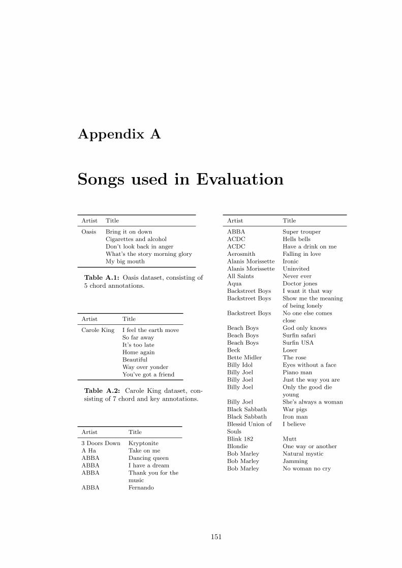
Appendix A
Songs used in Evaluation
Artist Title
Oasis Bring it on downCigarettes and alcoholDon’t look back in angerWhat’s the story morning gloryMy big mouth
Table A.1: Oasis dataset, consisting of5 chord annotations.
Artist Title
Carole King I feel the earth moveSo far awayIt’s too lateHome againBeautifulWay over yonderYou’ve got a friend
Table A.2: Carole King dataset, con-sisting of 7 chord and key annotations.
Artist Title
3 Doors Down KryptoniteA Ha Take on meABBA Dancing queenABBA I have a dreamABBA Thank you for the
musicABBA Fernando
Artist Title
ABBA Super trouperACDC Hells bellsACDC Have a drink on meAerosmith Falling in loveAlanis Morissette IronicAlanis Morissette UninvitedAll Saints Never everAqua Doctor jonesBackstreet Boys I want it that wayBackstreet Boys Show me the meaning
of being lonelyBackstreet Boys No one else comes
closeBeach Boys God only knowsBeach Boys Surfin safariBeach Boys Surfin USABeck LoserBette Midler The roseBilly Idol Eyes without a faceBilly Joel Piano manBilly Joel Just the way you areBilly Joel Only the good die
youngBilly Joel She’s always a womanBlack Sabbath War pigsBlack Sabbath Iron manBlessid Union of I believeSoulsBlink 182 MuttBlondie One way or anotherBob Marley Natural mysticBob Marley JammingBob Marley No woman no cry
151
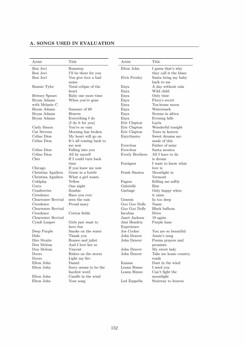
A. SONGS USED IN EVALUATION
Artist Title
Bon Jovi RunawayBon Jovi I’ll be there for youBon Jovi You give love a bad
nameBonnie Tyler Total eclipse of the
heartBritney Spears Baby one more timeBryan Adams When you’re gonewith Melanie CBryan Adams Summer of 69Bryan Adams HeavenBryan Adams Everything I do
(I do it for you)Carly Simon You’re so vainCat Stevens Morning has brokenCeline Dion My heart will go onCeline Dion It’s all coming back to
me nowCeline Dion Falling into youCeline Dion All by myselfCher If I could turn back
timeChicago If you leave me nowChristina Aguilera Genie in a bottleChristina Aguilera What a girl wantsColdplay YellowCorrs One nightCranberries ZombieCreedence Have you everClearwater Revival seen the rainCreedence Proud maryClearwater RevivalCreedence Cotton fieldsClearwater RevivalCyndi Lauper Girls just want to
have funDeep Purple Smoke on the waterDido Thank youDire Straits Romeo and julietDon Mclean And I love her soDon Mclean VincentDoors Riders on the stormDoors Light my fireElton John DanielElton John Sorry seems to be the
hardest wordElton John Candle in the windElton John Your song
Artist Title
Elton John I guess that’s whythey call it the blues
Elvis Presley Santa bring my babyback to me
Enya A day without rainEnya Wild childEnya Only timeEnya Flora’s secretEnya Tea-house moonEnya WatermarkEnya Storms in africaEnya Evening fallsEric Clapton LaylaEric Clapton Wonderful tonightEric Clapton Tears in heavenEurythmics Sweet dreams are
made of thisEverclear Father of mineEverclear Santa monicaEverly Brothers All I have to do
is dreamForeigner I want to know what
love isFrank Sinatra Moonlight in
VermontFugees Killing me softlyGabrielle RiseGarbage Only happy when
it rainsGenesis In too deepGoo Goo Dolls NameGoo Goo Dolls Black balloonIncubus DriveJanet Jackson 19 againJimi Hendrix Purple hazeExperienceJoe Cocker You are so beautifulJohn Denver Annie’s songJohn Denver Poems prayers and
promisesJohn Denver My sweet ladyJohn Denver Take me home country
roadsKansas Dust in the windLeann Rimes I need youLeann Rimes Can’t fight the
moonlightLed Zeppelin Stairway to heaven
152
Artist Title
Lionel Richie Endless loveLive I aloneMadonna Take a bowMariah Carey One sweet dayMariah Carey HeroMariah Carey Anytime you need
a friendMariah Carey Without youMetallica Nothing else mattersMichael Jackson Heal the worldMichael Jackson Beat itMike Oldfield Moonlight shadowMuse UnintendedNatalie Imbruglia TornNeil Diamond Sweet carolineNeil Diamond Red red wineNeil Diamond ShiloNeil Diamond Play meNeil Diamond Song sung blueNeil Diamond I am I saidNeil Sedaka Love will keep us
togetherNeil Sedaka Laughter in the rainNirvana Smells like teen spiritNo Doubt Just a girlNo Doubt Don’t speakNsync Bye bye byeNsync This I promise youO Town All or nothingOasis WonderwallOffspring Self esteemOlivia Newton John If you love meOlivia Newton John I honestly love youPapa Roach Last resortPaul Simon Bridge over troubled
waterPaul Simon The sound of silencePeter Gabriel SteamPhil Collins I wish it would
rain downPhil Collins In the air tonightPolice Message in a bottlePolice Every breath you
takePolice RoxannePresidents of the LumpUSA
Artist Title
Procol Harum A whiter shadeof pale
R Kelly I believe I can flyRadiohead Karma policeRem Everybody hurtsRichard Marx Right here waitingRicky Martin Livin la vida locaRod Stewart SailingRod Stewart Have i told you latelyRolling Stones Honky tonk womanRolling Stones Beast of burdenRoy Orbison Blue bayouRoy Orbison CryingRoy Orbison Oh pretty womanSarah Mclachlan AdiaSarah Mclachlan AngelSelena Dreaming of youShaggy AngelSimon and El condor pasa
(If I could)GarfunkelSimon and CeciliaGarfunkelSimon and The boxerGarfunkelSixpence None Kiss meThe RicherSoft Cell Tainted loveSoundgarden Black hole sunSpice Girls 2 become 1Stevie Wonder Sir dukeStevie Wonder Isn’t she lovelyStevie Wonder You are the sunshine
of my lifeStevie Wonder SuperstitionSting Fields of goldSublime Don t pushSublime SanteriaSurvivor Eye of the tigerTemple Of The Dog Hunger strikeThird Eye Blind Semi-charmed lifeTom Petty I won’t back downU2 With or without youVan Halen JumpVan Morrison Brown eyed girlVengaboys We’re going to IbizaWeezer El scorchoWeezer Hash pipe
153

A. SONGS USED IN EVALUATION
Artist Title
Weezer Island in the sunWhitney Houston Greatest love of all
Table A.3: USpop dataset, consistingof 193 chord annotations.
Artist Title
The Beatles I saw her standing thereMiseryAnna go to himChainsBoysAsk me whyPlease please meLove me doP.S. I love youBaby it’s youDo you want to knowa secretA taste of honeyThere’s a placeTwist and shoutIt won’t be longAll I’ve got to doAll my lovingDon’t bother meLittle childTill there was youPlease mister postmanRoll over beethovenHold me tightYou really got a holdon meI wanna be your manDevil in her heartNot a second timeMoney that’s what I wantA hard day’s nightI should have known betterIf I fellI’m happy just to dancewith youAnd I love herTell me whyCan’t buy me love
Artist Title
Any time at allI’ll cry insteadThings we said todayWhen I get homeYou can’t do thatI’ll be backNo replyI’m a loserBaby’s in blackRock and roll musicI’ll follow the sunMr moonlightKansas city hey heyEight days a weekWords of loveHoney don’tEvery little thingI don’t want to spoil the partyWhat you’re doingEverybody s trying to be my babyHelpThe night beforeYou’ve got to hide your love awayI need youAnother girlYou’re going to lose that girlTicket to rideAct naturallyIt’s only loveYou like me too muchTell me what you seeI’ve just seen a faceYesterdayDizzy miss lizzyDrive my carNorwegian wood (this bird has flown)You won’t see meNowhere manThink for yourselfThe wordMichelleWhat goes onGirlI’m looking through youIn my lifeWaitIf I needed someoneRun for your life
154
Artist Title
TaxmanEleanor RigbyI’m only sleepingLove you toHere there and everywhereYellow submarineShe said she saidGood day sunshineAnd your bird can singFor no oneDoctor RobertI want to tell youGot to get you into my lifeTomorrow never knowsSgt. Pepper’s lonely hearts clubbandWith a little help from myfriendsLucy in the sky withdiamondsGetting betterFixing a holeShe’s leaving homeBeing for the benefit ofMr KiteWithin you without youWhen I’m sixty-fourLovely RitaGood morning good morningSgt. pepper’s lonely hearts clubband (reprise)A day in the lifeMagical mystery tourThe fool on the hillFlyingBlue jay wayYour mother should knowI am the walrusHello goodbyeStrawberry fields foreverPenny laneBaby you’re a rich manAll you need is loveBack in the USSRDear prudenceGlass onionOb-la-di ob-la-daWild honey pie
Artist Title
The continuing story of bungalowBillWhile my guitar gently weepsHappiness is a warm gunMartha my dearI’m so tiredBlackbirdPiggiesRocky raccoonDon’t pass me byWhy don’t we do it in the roadI willJuliaBirthdayYer bluesMother nature’s sonEverybody’s got something to hideexcept me and my monkeySexy sadieHelter skelterLong long longRevolution 1Honey pieSavoy truffleCry baby cryGood nightCome togetherSomethingMaxwell’s silver hammerOh darlingOctopus’s gardenI want you (she’s so heavy)Here comes the sunBecauseYou never give me your moneySun kingMean Mr MustardPolythene PamShe came in through the bathroomwindowGolden slumbersCarry that weightThe endHer majestyTwo of usDig a ponyAcross the universeI me mine
155
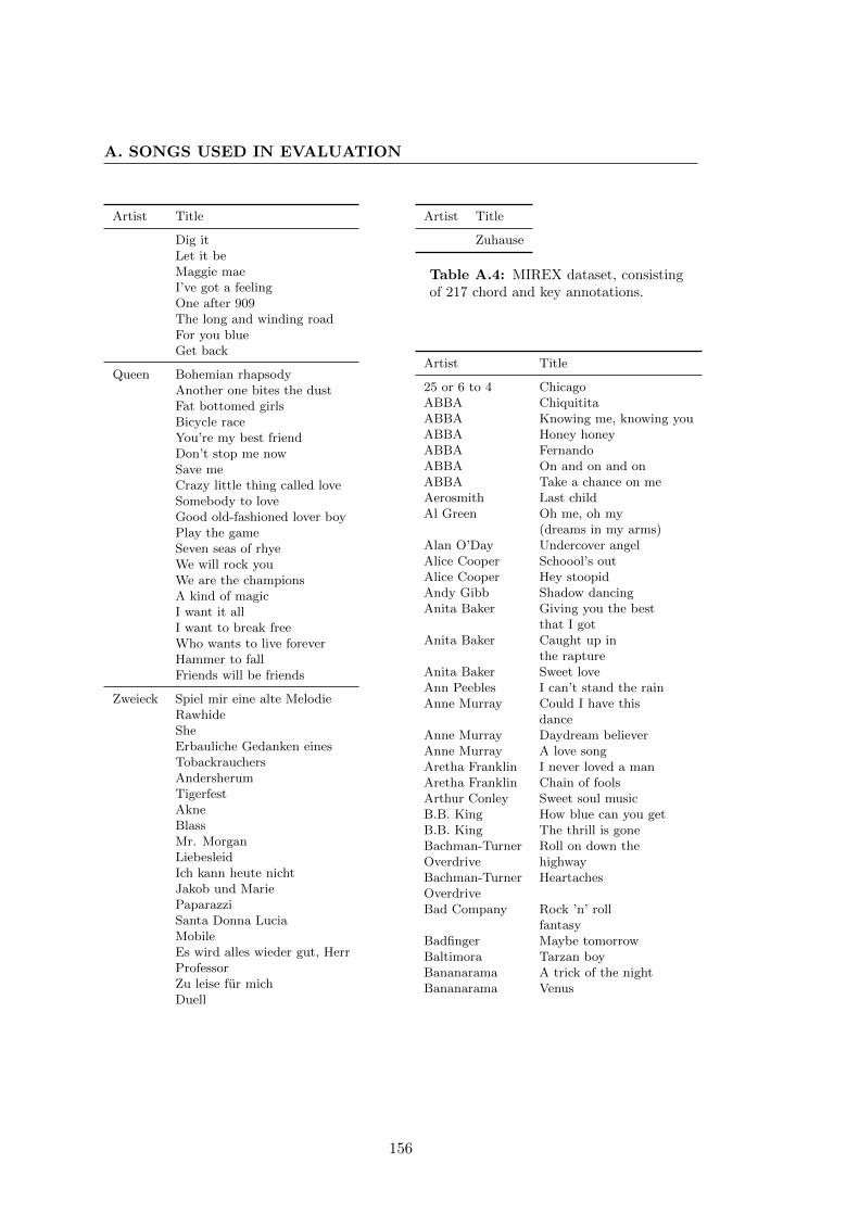
A. SONGS USED IN EVALUATION
Artist Title
Dig itLet it beMaggie maeI’ve got a feelingOne after 909The long and winding roadFor you blueGet back
Queen Bohemian rhapsodyAnother one bites the dustFat bottomed girlsBicycle raceYou’re my best friendDon’t stop me nowSave meCrazy little thing called loveSomebody to loveGood old-fashioned lover boyPlay the gameSeven seas of rhyeWe will rock youWe are the championsA kind of magicI want it allI want to break freeWho wants to live foreverHammer to fallFriends will be friends
Zweieck Spiel mir eine alte MelodieRawhideSheErbauliche Gedanken einesTobackrauchersAndersherumTigerfestAkneBlassMr. MorganLiebesleidIch kann heute nichtJakob und MariePaparazziSanta Donna LuciaMobileEs wird alles wieder gut, HerrProfessorZu leise fur michDuell
Artist Title
Zuhause
Table A.4: MIREX dataset, consistingof 217 chord and key annotations.
Artist Title
25 or 6 to 4 ChicagoABBA ChiquititaABBA Knowing me, knowing youABBA Honey honeyABBA FernandoABBA On and on and onABBA Take a chance on meAerosmith Last childAl Green Oh me, oh my
(dreams in my arms)Alan O’Day Undercover angelAlice Cooper Schoool’s outAlice Cooper Hey stoopidAndy Gibb Shadow dancingAnita Baker Giving you the best
that I gotAnita Baker Caught up in
the raptureAnita Baker Sweet loveAnn Peebles I can’t stand the rainAnne Murray Could I have this
danceAnne Murray Daydream believerAnne Murray A love songAretha Franklin I never loved a manAretha Franklin Chain of foolsArthur Conley Sweet soul musicB.B. King How blue can you getB.B. King The thrill is goneBachman-Turner Roll on down theOverdrive highwayBachman-Turner HeartachesOverdriveBad Company Rock ’n’ roll
fantasyBadfinger Maybe tomorrowBaltimora Tarzan boyBananarama A trick of the nightBananarama Venus
156

Artist Title
Barbara Lewis Hello strangerBarbara Streisand PeopleBarry White You’re the first,
the last, myeverything
Beastie Boys Brass monkeyBeautiful Gordon lightfootBen E. King AmorBertha Tillman Oh my angelBette Midler The roseBilly Idol Flesh for fantasyBilly Idol White weddingBilly Idol Catch my fallBilly Idol Hot in the cityBilly Joel PressureBilly Joel Just the way you
areBilly Joel Don’t ask me whyBilly Preston With you I’m born
againBilly Squier Don’t say you love
meBilly Squier The strokeBing Crosby Silent nightBiz Markie Just a friendBlondie One way or
anotherBlue Eyes Cryin’ Willie nelsonBo Diddley You can’t judge a
book by the coverBob Dylan Gotta serve
somebodyBob Seger Old time rock &
rollBob Seger Like a rockBob Seger & The Silver Trying to live myBullet Band life without youBobbi Martin I love you soBobby Bare Detroit cityBobby Womack That’s the way I
feel about chaBobby Womack Sweet Caroline (good
times never seemedso good)
Bonnie Raitt Nick of timeBoston Feelin’ satisfiedBoyz II Men Motown phillyBread If
Artist Title
Bread Sweet surrenderBrenda Lee Sweet nothin’sBrenda Lee As usualBrenda Lee Dum dumBrenda Lee Losing youBrenda Lee Heart in handBrenda Lee Too many riversBrenda Lee Everybody loves me
but youBrenda Lee Coming on strongBrother Jack McDuff Theme from electric
surfboardBrownsville Station Smokin’ in the
boys roomBruce Channel Hey babyCandi Staton Young hearts run
freeCanned Heat Let’s work togetherCanned Heat On the road againCarl Carlton Everlasting loveCharlie Rich A very special
love songCheap Trick I want you to
want meCheap Trick Dream policeCheap Trick Stop this gameCheap Trick SurrenderCher Just like Jesse JamesCher If I could turn
back timeChicago Along comes a
womanChicago Feelin’ stronger
every dayChicago Old daysChico DeBarge Talk to meChiffons Swing talkin’ guyChubby Checker The twistChuck Berry Sweet little
rock n’ rollChuck Berry Almost grownClarence Carter PatchesClarence Carter Too weak to
fightCliff Richard CarrieCommodores StillCorey Hart In your soul
157
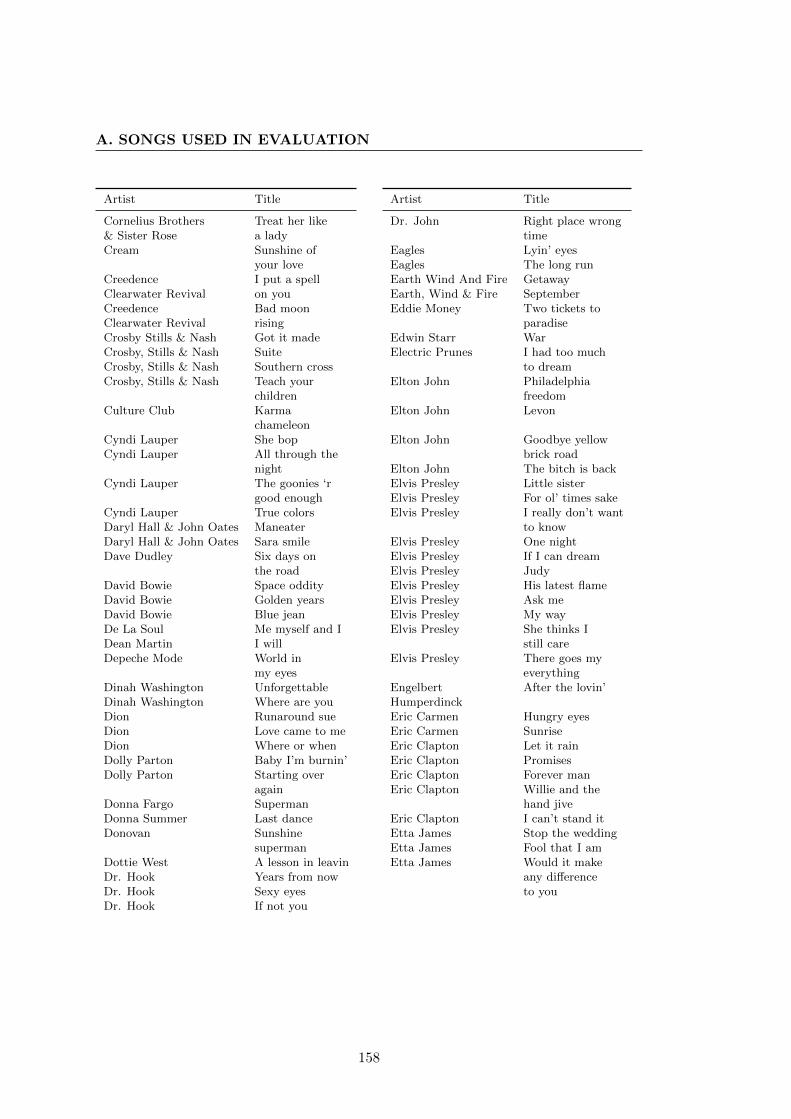
A. SONGS USED IN EVALUATION
Artist Title
Cornelius Brothers Treat her like& Sister Rose a ladyCream Sunshine of
your loveCreedence I put a spellClearwater Revival on youCreedence Bad moonClearwater Revival risingCrosby Stills & Nash Got it madeCrosby, Stills & Nash SuiteCrosby, Stills & Nash Southern crossCrosby, Stills & Nash Teach your
childrenCulture Club Karma
chameleonCyndi Lauper She bopCyndi Lauper All through the
nightCyndi Lauper The goonies ‘r
good enoughCyndi Lauper True colorsDaryl Hall & John Oates ManeaterDaryl Hall & John Oates Sara smileDave Dudley Six days on
the roadDavid Bowie Space oddityDavid Bowie Golden yearsDavid Bowie Blue jeanDe La Soul Me myself and IDean Martin I willDepeche Mode World in
my eyesDinah Washington UnforgettableDinah Washington Where are youDion Runaround sueDion Love came to meDion Where or whenDolly Parton Baby I’m burnin’Dolly Parton Starting over
againDonna Fargo SupermanDonna Summer Last danceDonovan Sunshine
supermanDottie West A lesson in leavinDr. Hook Years from nowDr. Hook Sexy eyesDr. Hook If not you
Artist Title
Dr. John Right place wrongtime
Eagles Lyin’ eyesEagles The long runEarth Wind And Fire GetawayEarth, Wind & Fire SeptemberEddie Money Two tickets to
paradiseEdwin Starr WarElectric Prunes I had too much
to dreamElton John Philadelphia
freedomElton John Levon
Elton John Goodbye yellowbrick road
Elton John The bitch is backElvis Presley Little sisterElvis Presley For ol’ times sakeElvis Presley I really don’t want
to knowElvis Presley One nightElvis Presley If I can dreamElvis Presley JudyElvis Presley His latest flameElvis Presley Ask meElvis Presley My wayElvis Presley She thinks I
still careElvis Presley There goes my
everythingEngelbert After the lovin’HumperdinckEric Carmen Hungry eyesEric Carmen SunriseEric Clapton Let it rainEric Clapton PromisesEric Clapton Forever manEric Clapton Willie and the
hand jiveEric Clapton I can’t stand itEtta James Stop the weddingEtta James Fool that I amEtta James Would it make
any differenceto you
158
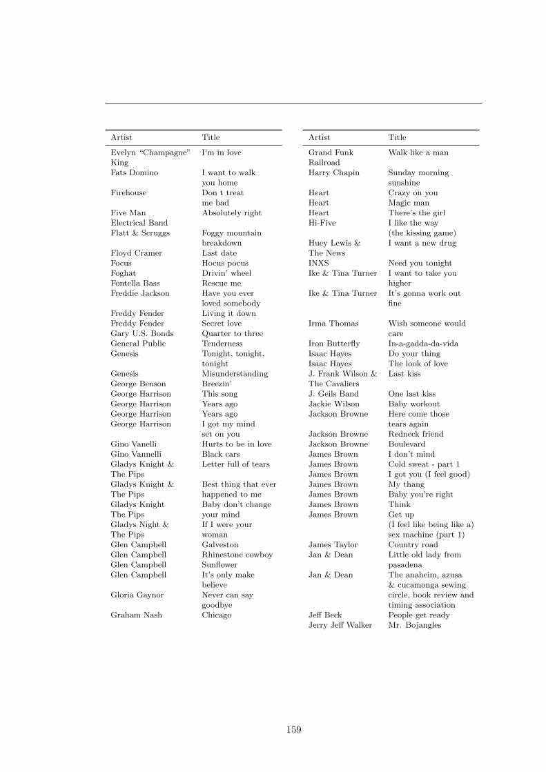
Artist Title
Evelyn “Champagne” I’m in loveKingFats Domino I want to walk
you homeFirehouse Don t treat
me badFive Man Absolutely rightElectrical BandFlatt & Scruggs Foggy mountain
breakdownFloyd Cramer Last dateFocus Hocus pocusFoghat Drivin’ wheelFontella Bass Rescue meFreddie Jackson Have you ever
loved somebodyFreddy Fender Living it downFreddy Fender Secret loveGary U.S. Bonds Quarter to threeGeneral Public TendernessGenesis Tonight, tonight,
tonightGenesis MisunderstandingGeorge Benson Breezin’George Harrison This songGeorge Harrison Years agoGeorge Harrison Years agoGeorge Harrison I got my mind
set on youGino Vanelli Hurts to be in loveGino Vannelli Black carsGladys Knight & Letter full of tearsThe PipsGladys Knight & Best thing that everThe Pips happened to meGladys Knight Baby don’t changeThe Pips your mindGladys Night & If I were yourThe Pips womanGlen Campbell GalvestonGlen Campbell Rhinestone cowboyGlen Campbell SunflowerGlen Campbell It’s only make
believeGloria Gaynor Never can say
goodbyeGraham Nash Chicago
Artist Title
Grand Funk Walk like a manRailroadHarry Chapin Sunday morning
sunshineHeart Crazy on youHeart Magic manHeart There’s the girlHi-Five I like the way
(the kissing game)Huey Lewis & I want a new drugThe NewsINXS Need you tonightIke & Tina Turner I want to take you
higherIke & Tina Turner It’s gonna work out
fine
Irma Thomas Wish someone wouldcare
Iron Butterfly In-a-gadda-da-vidaIsaac Hayes Do your thingIsaac Hayes The look of loveJ. Frank Wilson & Last kissThe CavaliersJ. Geils Band One last kissJackie Wilson Baby workoutJackson Browne Here come those
tears againJackson Browne Redneck friendJackson Browne BoulevardJames Brown I don’t mindJames Brown Cold sweat - part 1James Brown I got you (I feel good)James Brown My thangJames Brown Baby you’re rightJames Brown ThinkJames Brown Get up
(I feel like being like a)sex machine (part 1)
James Taylor Country roadJan & Dean Little old lady from
pasadenaJan & Dean The anaheim, azusa
& cucamonga sewingcircle, book review andtiming association
Jeff Beck People get readyJerry Jeff Walker Mr. Bojangles
159
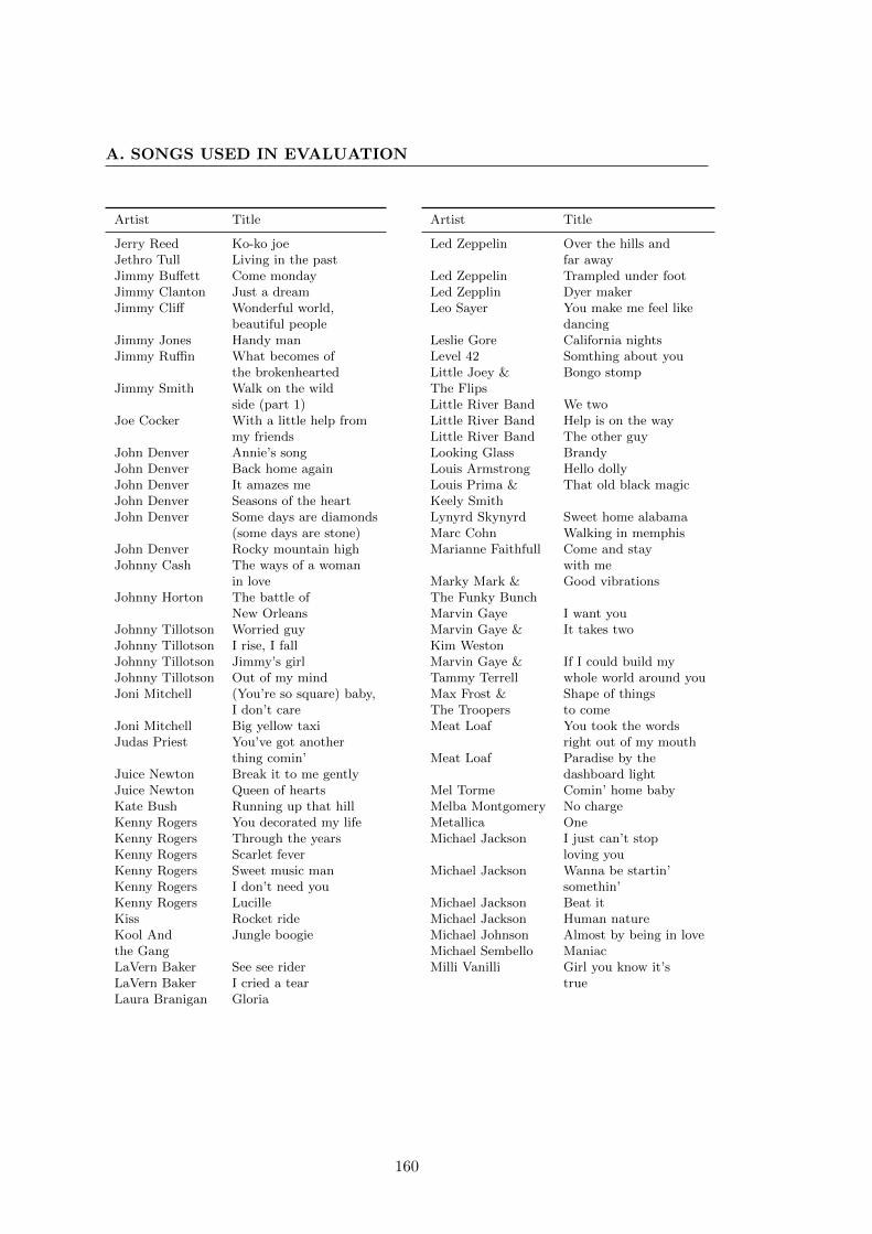
A. SONGS USED IN EVALUATION
Artist Title
Jerry Reed Ko-ko joeJethro Tull Living in the pastJimmy Buffett Come mondayJimmy Clanton Just a dreamJimmy Cliff Wonderful world,
beautiful peopleJimmy Jones Handy manJimmy Ruffin What becomes of
the brokenheartedJimmy Smith Walk on the wild
side (part 1)Joe Cocker With a little help from
my friendsJohn Denver Annie’s songJohn Denver Back home againJohn Denver It amazes meJohn Denver Seasons of the heartJohn Denver Some days are diamonds
(some days are stone)John Denver Rocky mountain highJohnny Cash The ways of a woman
in loveJohnny Horton The battle of
New OrleansJohnny Tillotson Worried guyJohnny Tillotson I rise, I fallJohnny Tillotson Jimmy’s girlJohnny Tillotson Out of my mindJoni Mitchell (You’re so square) baby,
I don’t careJoni Mitchell Big yellow taxiJudas Priest You’ve got another
thing comin’Juice Newton Break it to me gentlyJuice Newton Queen of heartsKate Bush Running up that hillKenny Rogers You decorated my lifeKenny Rogers Through the yearsKenny Rogers Scarlet feverKenny Rogers Sweet music manKenny Rogers I don’t need youKenny Rogers LucilleKiss Rocket rideKool And Jungle boogiethe GangLaVern Baker See see riderLaVern Baker I cried a tearLaura Branigan Gloria
Artist Title
Led Zeppelin Over the hills andfar away
Led Zeppelin Trampled under footLed Zepplin Dyer makerLeo Sayer You make me feel like
dancingLeslie Gore California nightsLevel 42 Somthing about youLittle Joey & Bongo stompThe FlipsLittle River Band We twoLittle River Band Help is on the wayLittle River Band The other guyLooking Glass BrandyLouis Armstrong Hello dollyLouis Prima & That old black magicKeely SmithLynyrd Skynyrd Sweet home alabamaMarc Cohn Walking in memphisMarianne Faithfull Come and stay
with meMarky Mark & Good vibrationsThe Funky BunchMarvin Gaye I want youMarvin Gaye & It takes twoKim WestonMarvin Gaye & If I could build myTammy Terrell whole world around youMax Frost & Shape of thingsThe Troopers to comeMeat Loaf You took the words
right out of my mouthMeat Loaf Paradise by the
dashboard lightMel Torme Comin’ home babyMelba Montgomery No chargeMetallica OneMichael Jackson I just can’t stop
loving youMichael Jackson Wanna be startin’
somethin’Michael Jackson Beat itMichael Jackson Human natureMichael Johnson Almost by being in loveMichael Sembello ManiacMilli Vanilli Girl you know it’s
true
160
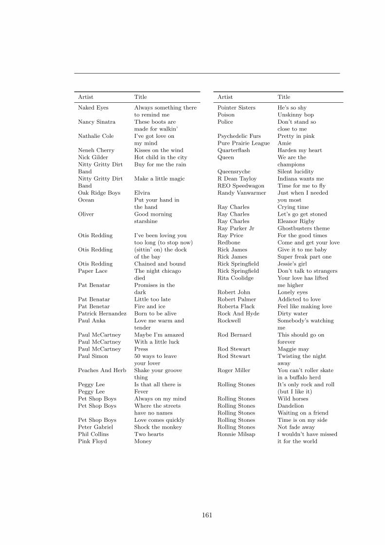
Artist Title
Naked Eyes Always something thereto remind me
Nancy Sinatra These boots aremade for walkin’
Nathalie Cole I’ve got love onmy mind
Neneh Cherry Kisses on the windNick Gilder Hot child in the cityNitty Gritty Dirt Buy for me the rainBandNitty Gritty Dirt Make a little magicBandOak Ridge Boys ElviraOcean Put your hand in
the handOliver Good morning
starshine
Otis Redding I’ve been loving youtoo long (to stop now)
Otis Redding (sittin’ on) the dockof the bay
Otis Redding Chained and boundPaper Lace The night chicago
diedPat Benatar Promises in the
darkPat Benatar Little too latePat Benetar Fire and icePatrick Hernandez Born to be alivePaul Anka Love me warm and
tenderPaul McCartney Maybe I’m amazedPaul McCartney With a little luckPaul McCartney PressPaul Simon 50 ways to leave
your loverPeaches And Herb Shake your groove
thingPeggy Lee Is that all there isPeggy Lee FeverPet Shop Boys Always on my mindPet Shop Boys Where the streets
have no namesPet Shop Boys Love comes quicklyPeter Gabriel Shock the monkeyPhil Collins Two heartsPink Floyd Money
Artist Title
Pointer Sisters He’s so shyPoison Unskinny bopPolice Don’t stand so
close to mePsychedelic Furs Pretty in pinkPure Prairie League AmieQuarterflash Harden my heartQueen We are the
championsQueensryche Silent lucidityR Dean Tayloy Indiana wants meREO Speedwagon Time for me to flyRandy Vanwarmer Just when I needed
you mostRay Charles Crying timeRay Charles Let’s go get stonedRay Charles Eleanor RigbyRay Parker Jr Ghostbusters themeRay Price For the good timesRedbone Come and get your loveRick James Give it to me babyRick James Super freak part oneRick Springfield Jessie’s girlRick Springfield Don’t talk to strangersRita Coolidge Your love has lifted
me higherRobert John Lonely eyesRobert Palmer Addicted to loveRoberta Flack Feel like making loveRock And Hyde Dirty waterRockwell Somebody’s watching
meRod Bernard This should go on
foreverRod Stewart Maggie mayRod Stewart Twisting the night
awayRoger Miller You can’t roller skate
in a buffalo herdRolling Stones It’s only rock and roll
(but I like it)Rolling Stones Wild horsesRolling Stones DandelionRolling Stones Waiting on a friendRolling Stones Time is on my sideRolling Stones Not fade awayRonnie Milsap I wouldn’t have missed
it for the world
161

A. SONGS USED IN EVALUATION
Artist Title
Roxette The lookRoxy Dance awayRoy Orbison Cry softly lonely oneRun-D.M.C. Walk this wayRush The spirit of radioSammy Hagar Give to liveSammy Hager I can’t drive 55The Animals San Franciscan
nightsSantana Evil waysSanto & Johnny Sleep walkSea Of Heartbreak Don gibsonShirley Brown Woman to womanSimple Minds Sanctify yourselfSimon & Mrs. RobinsonGarfunkelSinead O Connor The emperor’s
new clothesSly & The Family Hot fun in the
summertimeStoneSmokey Robinson Cruisin’Snap The powerSoft Cell Tainted loveSonny & Cher All I ever need is youSpandau Ballet TrueSteppenwolf Born to be wildSteve Miller Band The jokerStevie B Because I love youStevie Wonder Higher groundStevie Wonder If you really love meStevie Wonder That girlStevie Wonder Do I doSting If you love somebody
set them freeStyx Fooling yourself (the
angry young man)Swingin’ Medallions Double shot
(of my baby’s love)Talking Heads And she wasTalking Heads Burning down
the houseTanya Tucker Here’s some loveTeddy Pendergrass I don’t love you
anymoreTen Years After I’d love to change
the worldThe 5th Dimension Never my love
Artist Title
The 5th Dimension (Last night) I didn’tget to sleep at all
The 5th Dimension If I could reach youThe Allan Parsons Eye in the skyProjectThe Allman Brothers Straight from the
heartThe Amboy Dukes Journey to the
center of the mindThe Band Life is a carnivalThe Beach Boys Still cruisinThe Beach Boys Sail on sailorThe Beach Boys In my roomThe Beach Boys Bluebirds over the
mountainThe Beach Boys WendyThe Beach Boys Surfin’ safari
The Beatles Do you want toknow a secret
The Beatles Come togetherThe Beatles Eight days a weekThe Beatles I saw her standing
thereThe Beginning of Funky nassauthe EndThe Box Tops Cry like a babyThe Buckinghams Kind of a dragThe Byrds Eight miles highThe Castaways Liar, liarThe Commodores EasyThe Commodores NightshiftThe Contours Do you love meThe Cowsills HairThe Crystals He’s a rebelThe Cure Just like heavenThe Doors Riders on the stormThe Drifters On broadwayThe Eagles Already goneThe Everly Brothers Walk right backThe Everly Brothers Bird dogThe Everly Brothers On the wings
of a nightingaleThe Falcons I found a loveThe Fifth Dimension Where do you
wanna goThe Fireballs Sugar shackThe Hollies Long dark road
162

Artist Title
The Hollies Carrie-anneThe Isley Brothers It’s your thingThe J. Geils Band Just can’t waitThe J. Geils Band Looking for a loveThe Jacksons Dancing machineThe Kendalls Heaven’s just a
sin awayThe Kinks Better thingsThe Kinks Till the end of
the dayThe Miracles Baby, baby
don’t cryThe Miracles I don’t blame you
at allThe Miracles I second that
emotionThe Moments Walk right inThe Music Machine The people in meThe O’Jays Love trainThe Osmonds One bad appleThe Power Station Some like it hotThe Rascals People got to be
freeThe Rembrandts SomeoneThe Righteous Unchained melodyBrothersThe Righteous Soul andBrothers inspirationThe Ritchie Family The best disco
in townThe Robert Cray Smoking gunBandThe Rolling Stones Tumbling diceThe Rolling Stones Honky tonk womenThe Rolling Stones Doo doo doo doo
dooThe Rolling Stones Going to a go-goThe Rolling Stones Miss youThe Ronettes Be my babyThe Sopwith Camel Hello helloThe Staple Singers City in the skyThe String-A-Longs WheelsThe Supremes Floy joyThe Supremes Stoned loveThe Tee Set Ma belle amieThe Temptations Ain’t too proud
to beg
Artist Title
The Temptations I wish it wouldrain
The Trammps Disco infernoThe Ventures PerfidiaThe Weather Girls It’s raining menThe Who Pinball wizardThe Who Happy jackThe Yardbirds Heart full of soulThe Yardbirds Shapes of thingsThe Youngbloods Get togetherTina Turner The bestTina Turner Private dancerTodd Rundgren A dream goes on foreverTom D Hall I loveTom Jones She’s a ladyTommy James Crystal blue persuasionTommy James Mony monyTracie Spencer This houseTracy Chapman Baby can I hold
youTwilight Zone Golden earringU2 With or without youUB40 Red red wineUB40 The way you do the
things you doUrban Dance Squad Deeper shade of soulVillage People In the navyWang Chung Dance hall daysWaylon Jennings Theme from the
dukes of hazzardWham! Wake me up before
you go-goWhitesnake Here I go againWilson Phillips Hold onWilson Pickett Don’t Knock
My Love - Pt. 1Wilson Pickett I found a true loveYaz SituationZZ Top La grange
Table A.5: Billboard dataset, consist-ing of 522 chord and key annotations.
163

A. SONGS USED IN EVALUATION
164
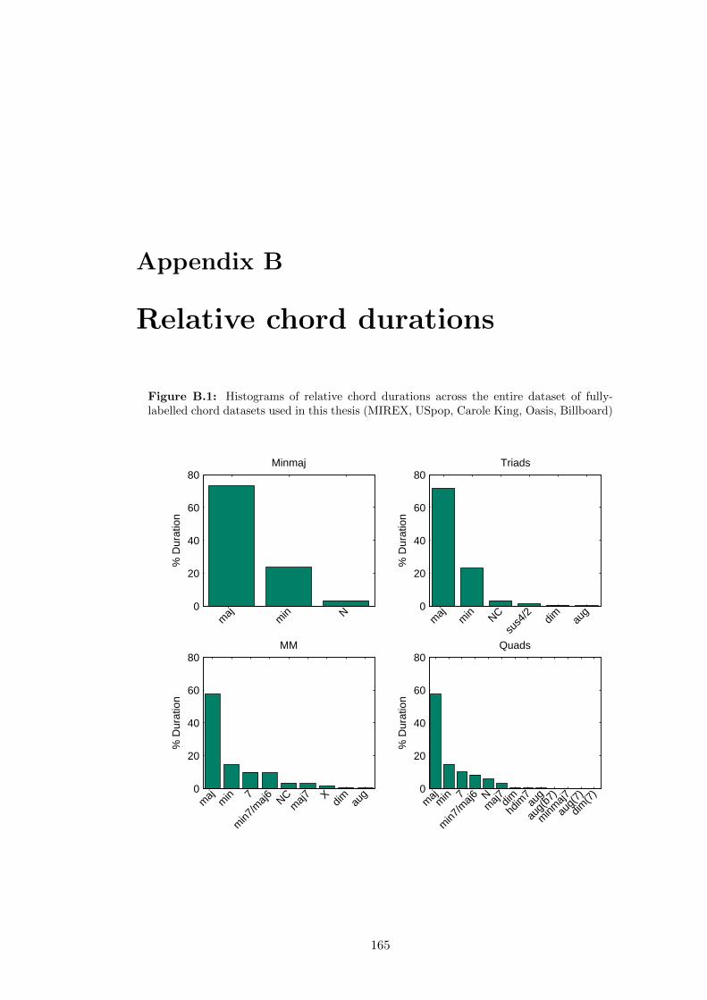
Appendix B
Relative chord durations
Figure B.1: Histograms of relative chord durations across the entire dataset of fully-labelled chord datasets used in this thesis (MIREX, USpop, Carole King, Oasis, Billboard)
0
20
40
60
80Minmaj
% D
urat
ion
maj
min N
0
20
40
60
80Triads
% D
urat
ion
maj
min NC
sus4
/2 dim aug
0
20
40
60
80MM
% D
urat
ion
maj
min 7
min7
/maj6 NC
maj7 X
dim aug 0
20
40
60
80Quads
% D
urat
ion
maj
min 7
min7
/maj6 N
maj7dim
hdim
7au
g
aug(
b7)
minm
aj7
aug(
7)
dim(7
)
165