a macro stress test model of credit risk for the brazilian ... · test of credit risk for the...

CHAPTER 29

A Macro Stress Test Model of Credit Risk for the Brazilian Banking Sector

FRANCISCO VAZQUEZ • BENJAMIN M. TABAK • MARCOS SOUTO

This chapter proposes a model to conduct a macro stress test of credit risk for the banking sector based on scenario analysis. We employ an origi-nal bank- level data set that splits bank credit portfolios into 21 granular categories, covering house hold and corporate loans. The results cor-

roborate the presence of a strong procyclical behavior of credit quality and show a robust negative relationship between the logistic transformation of NPLs and GDP growth, with a lag response up to three quarters. The results also indicate that the procyclical behavior of loan quality varies across credit types. This is novel in the literature and suggests that banks with larger exposures to highly procyclical credit types and economic sectors would tend to undergo sharper deterioration in the quality of their credit portfolios during an economic downturn. Lack of suffi cient port-folio granularity in macro stress testing fails to capture these eff ects and thus introduces a source of bias that tends to underestimate the tail losses stemming from the riskier banks in a system.

METHOD SUMMARY

Overview The model enables macro stress testing of credit risk based on scenario analysis.

Application • The stress test framework comprises three components that are integrated in sequence: (1) a macro vector autoregression model; (2) a micro logit panel; and (3) a credit value- at- risk (VaR) model based on the CreditRisk+ formulation.

• It is appropriate for situations where granular data at the portfolio level are available.

Nature of approach Econometric analysis.

Data requirements • Bank- level nonperforming loan (NPL) data that split bank credit portfolios in granular categories, covering house hold and corporate loans.

• Macro variables such as GDP growth, credit growth, and interest rates. • Information on distressed probabilities of default is estimated from the credit VaR model.

Strengths The model allows the simulation of credit risk at the bank level under distressed macroeconomic scenarios, while minimiz-ing portfolio aggregation bias.

Weaknesses • The model does not capture potential feedback eff ects between the banking system and the economy under distressed scenarios.

• In addition, the model implicitly assumes a linear, symmetric response of credit quality to macroeconomic conditions throughout the cycle, which may not be appropriate.

• The implementation requires granular data on NPLs at the bank level, split by sectors for corporate loans and by size (small, medium, and large) for house hold loans.

Tool • For the panel econometrics, the Stata script is available from the authors upon request. • For the credit VaR, the CreditRisk+ model is available with this book. • Contact authors: F. Vazquez and M. Souto.

Th is chapter was previously published in the Journal of Financial Stability (2012), Vol. 8, No. 2, pp. 69– 83 (Vazquez, Tabak, and Souto, 2012). Th e authors would like to thank Pedro Rodriguez, Rafael Romeu, Gilneu Vivan, seminar participants at the Central Bank of Brazil and IMF, two anonymous reviewers, and the journal editor Iftekhar Hasan for useful comments. Benjamin M. Tabak gratefully acknowledges fi nancial support from the CNPQ Foundation.

536-57355_IMF_StressTestHBk_ch04_3P.indd 453 11/5/14 12:22 AM

A Macro Stress Test Model of Credit Risk for the Brazilian Banking Sector 454

tive relationship between (the logit transformation of ) NPLs and GDP growth, with a lag response up to three quarters. Comparative static exercises indicate that a 2 percentage point drop in yearly GDP growth, which is akin to the maximum drop observed in Brazil during 1996– 2008, would cause a two- time increase in NPLs from their March 2009 levels, to about 7 percent. In addition, credit quality displays a strong inertial behavior across all credit types, with autoregressive co-effi cients implying that a 1 percentage point increase in NPLs in a given quarter produces a 0.4 percentage increase in NPLs in the next quarter. Credit to individuals, vehicles, and retail commerce was found to be relatively more sluggish.

Th e models also indicate substantial variations in the cycli-cal behavior of NPLs across credit types, with no statistically signifi cant diff erences across state- owned and private banks, suggesting that the results are not due to likely diff erences in credit origination practices across these two types of banks.3 At the same time, some credit types appeared to be more sensitive to changes in economic activity, particularly agriculture, sugar and alcohol, livestock, small consumer credit, and textiles. Consequently, the quality of these credit types would likely undergo more severe erosion under a protracted drop in eco-nomic activity. Banks with higher exposures to these credit types may need to be followed up more closely.

Overall, the stress tests suggest that the Brazilian bank-ing sector is well prepared to absorb the credit losses associ-ated with a set of distressed macroeconomic scenarios without threatening fi nancial stability. Four alternative macroeco-nomic scenarios, each one projected over two years, were analyzed. Th ese comprised a baseline refl ecting the expected path of GDP growth and three distressed scenarios that were deemed to be extreme but nevertheless likely under current circumstances. Overall, the results of the baseline scenario indicate that NPLs peak at 6.7 percent in the fourth quarter of 2010, before recovering. Th e simulated NPLs for the dis-tressed scenarios are higher than for the baseline. Th e more severe deterioration in credit quality is associated with a slow-down in GDP growth akin to two standard deviations below its 2001– 9 mean, with overall NPLs reaching a maximum of 8.5 percent, which is about a two- time increase from their starting levels.

Th e remainder of the chapter is structured as follows: Section 1 presents a brief literature review, whereas Section 2 discusses the methodology. Section 3 presents the empirical results. Finally, Section 4 concludes the chapter.

1. LITERATURE REVIEWSince the seminal works of Wilson (1997a, 1997b), which present a framework to examine credit risk under distressed macroeconomic conditions, several papers have applied macro

3 Recent literature for the Brazilian banking system suggests that there may be important diff erences across banks because of own ership (Tabak and Staub, 2007; Staub, da Silva e Souza, and Tabak, 2010; Tecles and Tabak, 2010; Tabak, Fazio, and Cajueiro, 2011).

Th ere has been a growing literature on stress testing in recent years. Th e importance of these exercises has been high-lighted by the recent crisis and the cascade of bank failures in many countries. A deep understanding of the resilience of a banking sector to adverse macroeconomic scenarios is of crucial importance for the proper evaluation of systemic risk and has a direct connection with the development of new regulatory and prudential tools.

Th is chapter describes a model to conduct a macro stress test of credit risk for the Brazilian banking sector based on scenario analysis. Th e proposed framework comprises three in de pen dent, yet complementary modules that are combined in sequence. Th e fi rst module uses time series econometrics to estimate the relationship between selected macroeconomic variables and uses the results to simulate distressed, internally consistent, macroeconomic scenarios spanning two years. Th e second module uses panel data econometrics to estimate the sensitivity of nonperforming loans (NPLs) to GDP growth and uses the results to simulate the evolution of credit quality for individual banks and credit types under distressed sce-narios.1 Th is module exploits a rich database that tracks the evolution of NPLs for 78 individual banks and 21 categories of credit for the 2001– 9 period.2 Th e third module uses the predicted NPLs as a proxy for distressed probabilities of de-fault (PDs) and combines this information with data on the exposures and concentration of bank credit (gross loans) port-folios to estimate tail credit losses, using a credit value- at- risk (VaR) framework.

Th is study makes three main contributions to the literature on stress testing. First, it exploits a rich partition of bank credit portfolios by borrower types (i.e., consumer versus corporates) and economic sectors and assesses the extent of diff erences in the sensitivity of credit quality to macroeconomic conditions across credit types. Second, it illustrates that macro stress test models based on insuffi ciently granular data on banks’ credit portfolios may be biased in a material way. In par tic u lar, mac-roeconomic stress test models based on undiff erentiated credit data may tend to underestimate the credit losses stemming from the highly procyclical credit types (and overestimate the losses associated with the relatively safer credit types). To the extent that the composition of bank credit portfolios varies across institutions, the use of insuffi ciently granular credit data would tend to underestimate the tail losses of riskier banks, which runs against prudent principles. Th ird, we present and discuss the results for the Brazilian banking system, which is one of the largest banking systems in Latin America.

Th e results corroborate the presence of a strong procycli-cal behavior of credit quality, as indicated by a robust nega-

1 NPLs for each credit type are computed as the ratio of loans past due in excess of 90 days relative to the total loans in the corresponding category.

2 Th e data come from information reported by the supervised institutions to the credit registry of the Central Bank of Brazil. In general, the credit portfolios analyzed in this study cover virtually all the bank credit to the private sector under market conditions. Th is represents about two- thirds of total bank credit, owing to the exclusion of credit operations granted under statutory conditions (the so- called directed lending).


Francisco Vazquez, Benjamin M. Tabak, and Marcos Souto 455

tressed macroeconomic scenarios, and the results are then mapped into banks’ solvency and aggregated to get a systemic picture. Possibly because of data constraints, however, bottom- up models fail to exploit granular data on the characteristics of individual banks’ credit portfolios (i.e., portfolio concentra-tion and loan per for mance by credit types).6

Our study contributes to this literature by presenting a macro stress test model of credit risk that combines the use of bank- level information with a granular partition of banks’ credit portfolios between consumer and corporate loans, classifying the former by size and the latter by economic sec-tors. In par tic u lar, we assess the sensitivity of credit quality to macroeconomic conditions using a bank- level data set that keeps track of 21 credit categories during 2001– 9. Th e estimated pa ram e ter vectors are used to simulate the evolu-tion of credit quality for individual banks and specifi c credit types, under adverse macroeconomic scenarios. Th is infor-mation is then combined using a credit portfolio approach to estimate the bank- specifi c capital needs conditional on the realization of the adverse macroeconomic scenarios.

Overall, the results suggest that the procyclical behavior of credit quality varies across credit types. By failing to account for these diff erences, current macro stress test models may be biased in a material way, underestimating the riskiness of banks that are more heavily exposed to highly procyclical credit types and economic sectors. We illustrate this bias by running par-allel simulations of bank- level NPLs under adverse macro-economic scenarios, using two approaches. Th e fi rst, akin to typical macro stress test models of credit risk, uses bank- level data on credit quality, without allowing for diff erences in the behavior of credit quality across credit types. Th e second, fol-lowing the approach presented in this study, exploits granular information on the characteristics of bank credit portfolios. Th e fi ndings provide strong evidence of a data aggregation bias that tends to underestimate the impact of macro shocks on the quality of bank credit portfolios. Papers reporting that banking systems were resilient to adverse macroeconomic sce-narios may have been infl uenced partly by this underestima-tion of credit risk.

2. METHODOLOGY

A. Overview of the methodology

Th e stress test framework presented in this chapter com-prises three components that are integrated in sequence:

• A macroeconomic model to estimate the relationship between selected macroeconomic variables with the help of times- series analysis. Th is model is used to simulate distressed, internally consistent, macroeco-nomic scenarios, projected over two years.

6 Th ere is to date little research using the bottom- up approach. Interest-ing examples are the works of Coffi net and Martin (2009) and Coffi net and Lin (2010), which perform a bottom- up stress test for French banks profi tability and income subcomponents, respectively.

stress test tools to assess the resilience of various banking sys-tems to adverse macroeconomic shocks (Berkowitz, 1999; Pe-sola, 2001, 2005; Frøyland and Larsen, 2002; Hoggarth and Whitley, 2003; Gerlach, Peng, and Shu, 2004; Sorge, 2004; Virolainen, 2004; Barnhill, Souto, and Tabak, 2006; van den End, Hoeberichts, and Tabbae, 2006; Boss and others, 2007; and Misina and Tessier, 2008, among others).4 In this litera-ture, the main objective is to gauge the vulnerability of a portfolio (market, credit, or both) to adverse macroeconomic scenarios or to extreme but plausible events or shocks. Th e objective of such tests is to make risks more transparent, as-sessing the potential losses of a given portfolio under abnor-mal markets. Th ese tools are commonly used by fi nancial institutions as part of their internal models and management systems and to inform decisions regarding risk taking and capital allocation. Besides, these tools have become used in-creasingly by fi nancial regulators to evaluate the soundness of the fi nancial systems under their control.

Typically, macro stress tests of credit risk involve three major tasks: fi rst, the development of a model to capture the interrelationships between selected macroeconomic and fi nan-cial variables; second, the calibration of pa ram e ter vectors linking macroeconomic and fi nancial variables to specifi c mea sures of loan per for mance; third, the design of adverse macroeconomic scenarios and the computation of their impact on credit quality and banks’ solvency. Usually, the macro-economic variables used in stress test models include mea sures of economic activity (i.e., GDP growth, the output gap, and unemployment) and mea sures of monetary conditions and key prices (i.e., interest rate, exchange rate, infl ation, money growth, and property prices).

Th e investigation of how adverse scenarios may aff ect asset quality and solvency in the banking sector can be done using two approaches: top- down or bottom- up. Th e fi rst one builds on aggregated data on bank credit portfolios, some-times split by credit types or economic sectors, and simulates evolution of aggregated credit quality under distressed macro scenarios with the help of time-series analysis (see, e.g., Viro-lainen, 2004; and Wong, Choi, and Fong, 2006). A key short-coming of this approach is its limited capacity to assess the fi nancial conditions of individual institutions, which are fre-quently the focus of the analysis. Th e bottom- up approach ad-dresses this shortcoming by resorting to the use of bank- level data.5 Typically, models based on this approach use panel data econometrics to gauge the evolution of asset quality under dis-

4 See Sorge and Virolainen (2006) for an overview of stress test method-ologies. See also Illing and Liu (2006); Rodriguez and Trucharte (2007); Blank, Buch, and Neugebauer (2009); Castrén, Dées, and Za-her (2010); and Cardarelli, Elekdag, and Lall (2011). Foglia (2009) pro-vides a very interesting review of current approaches to stress testing employed by supervisory authorities.

5 An example is Duellmann and Erdelmeier (2009), who stress test the credit portfolio of German banks using a diff erent approach from ours (Merton- type multifactor credit risk model). Th e authors show that it is crucial to capture credit risk dependencies between sectors. Th e focus is on the automobile sector (key sector) and its interdependencies with other sectors.



events, including a substantial shock in 2002– 3, when the ref-erential interest rate shot up by almost 10 percentage points to 26.5 percent and the exchange rate depreciated from 2.3 to almost 4 Brazilian real (BRL) per U.S. dollar (USD). Th e memory of this shock is important to help model the dy-namics of the global fi nancial crisis, which also aff ected Bra-zil, particularly since the third quarter of 2008. Th e substantial contraction in GDP is an important consideration for the vector autoregression (VAR) specifi cation as it will, mechan-ically, force the factor to rebound in a way that may not be completely consistent with macroeconomic dynamics going forward. We present credit growth, GDP growth, and changes in the yield curve for the Brazilian economy in Figure 29.1.

Th e selected specifi cation captures linkages between GDP growth, credit growth, and changes in the slope of the domes-tic yield curve. We choose a parsimonious specifi cation given the relatively short length of the time series. Th e variables were selected after exploring the relationships between a larger set of macroeconomic variables restricting the factors to those that were statistically more relevant to the VAR specifi -cation, also yielding tighter error bands.8 Th e selected variables are defi ned as follows: (1) GDP growth, GDP, computed by taking the fi rst diff erence to the natural log of the seasonally

8 Th e set of variables used in the selection of the specifi cation include: the short- term policy rate (i.e., SELIC), the spread between bank lending and deposit rates, the U.S. yield curve (mea sured by the diff erence be-tween the seven- year and three- month Trea sury bill rates, the Chicago VIX index, the Emerging Market Bond Index (EMBI) spreads, a com-modity price index (proxied by the Commodity Research Bureau Index), the unemployment rate, and the exchange rate. We have estimated the correlation for slope between estimations with the 7 years and 3 months and 10 years and 3 months periods, and it is above 99 percent.

• A microeconomic model to assess the sensitivity of loan quality to macroeconomic conditions with the help of dynamic panel econometrics. Th e model is based on bank- level data, using separate equations for 21 credit types. Th e results are used to simulate the path of NPLs for each bank and for each of the 21 categories of credit, under the distressed macroeconomic sce-narios produced in the previous stage.

• A credit VaR model to estimate the banks’ capital needs to cover tail credit losses under the distressed scenarios. Th e model uses the simulated distributions of NPLs for each bank and credit type as a proxy for the distribution of distressed PDs and combines this information with data on the credit exposures of individual banks using the CreditRisk+ approach with the programs developed by Avesani and others (2006).

B. The macro model

Th e model outlined in this section uses times-series econo-metrics to capture the relationship between selected macro-economic variables. As mentioned before, the results are used to build distressed scenarios projected over two years.

Macroeconomic data on key target series are available at a quarterly frequency, from the fi rst quarter of 2001 to the fi rst quarter of 2009.7 Although the length of the time series is somewhat short, the period covers some important macro

7 Before 2001, we had the peg regime in exchange rate and a transition to the fl oating rate regime. After 2001, fl oating rate regime was in perma-nent regime.

–.1

–.05

0

.05

.1

2000q1 2003q1 2006q1 2009q1

Change in the slope of the yield curveFirst difference of log creditFirst difference of log GDP

Source: Authors.

Figure 29.1 Selected Macroeconomic Variables, First Diff erences, 2000– 9



growth and GDP growth, and there is a strong positive rela-tionship between the last two variables. Th ere is also evidence that the decline of GDP growth during the last quarter of 2008 and the fi rst quarter of 2009 was larger than otherwise explained by the interaction between the endogenous vari-ables included in the model, as indicated by the coeffi cient of the dummy variable, which is negative and statistically sig-nifi cant. Th e results also indicate that the domestic credit mar-kets were somehow isolated from the eff ects of the global fi nancial crisis, which is likely attributable to the strong ex-pansion of credit by state- owned banks to compensate for the collapse of credit growth by private banks during this period. Similar conclusions can be extracted from the results of a re-stricted VAR, presented in the right three columns. Postes-timation tests (not reported to save space) indicate that the models are stable and that the errors are not autocorrelated and pass standard normality tests. Th e impulse response func-tions, together with 95 percent confi dence error bands, are presented in Figure 29.2.

Th e fi rst diff erence of the slope of the yield curve would represent a change in the yield curve slope from one period to the next. Changes in yield curve slope are associated with investors’ perception about future monetary policy, vis-à- vis current interest rates. For example, if GDP decreases from one period to the next, investors may expect the interest rates to go down in the future, causing a drop in the slope of the yield curve.

C. The microeconomic model

Data on credit portfolios were gathered from the credit reg-istry of the Central Bank of Brazil, which contains rich in-formation on individual credit operations granted by the supervised banks. Th e registry covers the bulk of credit in the system, leaving aside operations lower than a minimum reporting threshold and credits granted by unsupervised en-tities (such as nonfi nancial corporations).10 Th e data used in this exercise, however, focus on lending granted with non-earmarked resources, which accounts for about 70 percent of total credit, as information on directed lending was not available.11 For the purposes of the analysis, the data were aggregated at the level of individual banks and classifi ed in 21 categories (Table 29.3). For each one, we have (1) total (gross) loans; (2) NPLs; (3) number of loan operations; (4) number of loan operations in default; and (5) (specifi c) loan- loss provisions.

Overall, the database covers the credit operations of 78 banks, at a quarterly frequency, between 2003:Q1 and 2009:Q1. Th e size of the credit portfolios included in the

10 It is important to highlight that the credit registry covers operations that represent more than 80 percent of the total volume of credit. Also, in Brazil most credit operations are performed within the regulated bank-ing system. Th erefore, the database is highly representative of the credit operations in Brazil.

11 Nonearmarked resources are credit granted by fi nancial institutions without implicit or explicit subsidies from the government.

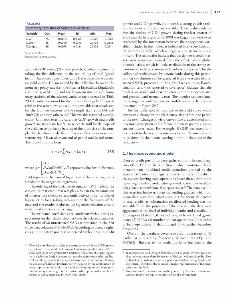
adjusted GDP series; (2) credit growth, Credit, computed by taking the fi rst diff erence to the natural log of total (gross) loans in bank credit portfolios; and (3) the slope of the domes-tic yield curve, YC, mea sured by the diff erence between the monetary policy rate (i.e., the Sistema Especial de Liquidação e Custodia, or SELIC) and the long- term interest rate. Sum-mary statistics of the selected variables are presented in Table 29.1. In order to control for the impact of the global fi nancial crisis in the system, we add a dummy variable that equals one for the last two quarters of the sample (i.e., 2008:Q4 and 2009:Q1) and zero otherwise.9 Th is variable is treated as exog-enous. Unit root tests indicate that GDP growth and credit growth are stationary but fail to reject the null for the slope of the yield curve, probably because of the short size of the sam-ple. We therefore use the fi rst diff erence of the series to achieve stationarity. All variables are end of period and in real terms. Th e model is of the form

yt = c + Asyt s +Bxt + t ,s=1

p

(29.1)

where y =D. ycD.Ln(Credit )D.Ln(GDP )

, D represents the fi rst diff erence,

Ln(·) represents the natural logarithm of the variables, and x stands for the exogenous regressors.

Th e ordering of the variables in equation (29.1) refl ects the conjecture that credit markets play a role in the transmission of interest rate shocks to economic activity. Th e number of lags is set to four, taking into account the frequency of the data and the results of alternative lag order selection criteria (which indicate two to fi ve lags).

Th e estimated coeffi cients are consistent with a priori ex-pectations on the relationship between the selected variables. Th e results of an unrestricted VAR are presented in the fi rst three data columns of Table 29.2. According to these, a tight-ening in monetary policy is associated with a drop in credit

9 We tried a number of variables to capture external eff ects (GDP growth in the United States and the Eu ro pe an Union, commodity prices, EMBI, VIX) with poor (insignifi cant) t- statistics. Th erefore, this may suggest that a decline in foreign demand was not the main reason aff ecting Bra-zil. One likely cause is the sharp exchange rate depreciation following the collapse of Lehman Brothers, partly triggered by the combination of heavy capital outfl ows with the sudden unwinding of corporate posi-tions in foreign exchange rate derivatives, which prompted a number of monetary policy responses by the Central Bank.

TABLE 29.1

Summary Statistics of Selected VariablesVariable Obs Mean SD Min Max

D.yc 35 0.0005 0.0164 0.0507 0.0514D.Lncr 35 0.0399 0.0318 0.0736 0.0878D.Lngdp 35 0.0075 0.0124 0.0372 0.0241

Source: Authors.Note: Obs = observations.



sampled period, which is relatively high considering the favor-able macroeconomic environment and the rapid expansion of credit portfolios. Furthermore, credit quality has been dis-persed across banks and throughout time, as indicated by the size of the standard deviations of NPLs, which are gener-ally two to three times larger than their corresponding mean values (Table 29.5). Th e extent of the dispersion of credit quality and the severity of loan nonper for mance in some in-stitutions is also illustrated by the NPL ratios of banks in the 90th percentile of the distribution, which exceeded 10 per-cent in many sectors. Across credit types, the higher average rates of NPLs have been associated with credit to individuals (particularly small- and medium- sized loans), fi rms operating in the ser vices sector, producers of livestock, and electric and electronic equipment.

Th e evolution of NPLs was also diverse across bank types. Overall, state- owned banks displayed better loan quality dur-ing the sampled period, interrupted only by a sharp increase in NPLs on exposures to the petrochemical and food indus-

analysis is rather continuous throughout the sampled period (Table 29.4). Th e sample, however, is unbalanced because of the exit or merging of some banks and the incorporation of new ones. As of March 2009, the sample included 49 banks jointly accounting for about 85 percent of total bank credit.12 Th e time coverage was dictated by data availability. In par-tic u lar, the construction of time series going further back in time was not possible because of a change in accounts and data reporting defi nitions introduced in 2002. Th e quality of the data was deemed to be good. Several fi lters were ap-plied to identify potential inconsistencies, and a few data reporting issues were found to be (generally) associated with a specifi c subgroup of banks.

A look at the bank- level data indicates that credit quality has been relatively poor and extremely heterogeneous across credit types. Overall, NPLs averaged 3.6 percent during the

12 Credit is highly concentrated in Brazil, with the largest fi ve banks ac-counting for approximately 70 percent of total credit.

TABLE 29.2

Macro Model Specifi cationUnrestricted Model Restricted Model

Variable D_yc D_lncr D_lngdp D_yc D_lncr D_lngdp

LD.yc 0.594*** 0.575** 0.263*** 0.618*** 0.595*** 0.259***(0.000) (0.022) (0.004) (0.000) (0.007) (0.004)

L2D.yc 0.027 0.16 0.135 0.054(0.885) (0.580) (0.205) (0.536)

L3D.yc 0.089 0.178 0.207** 0.269***(0.605) (0.511) (0.038) (0.002)

L4D.yc 0.03 0.316 0.059(0.868) (0.261) (0.566)

LD.lncr 0.209** 0.391*** 0.148*** 0.239*** 0.306** 0.159***(0.013) (0.003) (0.002) (0.001) (0.014) (0.000)

L2D.lncr 0.167* 0.051 0.177*** 0.180*** 0.197* 0.197***(0.054) (0.705) (0.000) (0.006) (0.074) (0.000)

L3D.lncr 0.119 0.212 0.079 0.137* 0.315*** 0.065(0.162) (0.112) (0.106) (0.074) (0.008) (0.135)

L4D.lncr 0.264*** 0.261** 0.04 0.304*** 0.230**(0.001) (0.032) (0.371) (0.000) (0.028)

LD.lngdp 0.039 1.100*** 0.514*** 0.918*** 0.504***(0.856) (0.001) (0.000) (0.000) (0.000)

L2D.lngdp 0.182 1.129** 0.524*** 0.656* 0.482***(0.557) (0.020) (0.003) (0.089) (0.002)

L3D.lngdp 0.001 0.779* 0.425** 0.436***(0.997) (0.097) (0.014) (0.001)

L4D.lngdp 0.107 0.606 0.279* 0.304**(0.696) (0.159) (0.078) (0.019)

dummy_crisis 0.01 0.004 0.044*** 0.044***(0.280) (0.788) (0.000) (0.000)

Constant 0.002 0.009 0.008*** 0.001 0.014* 0.009***(0.674) (0.264) (0.005) (0.802) (0.061) (0.001)

Observations 31 31 31 31 31 31R 0.63 0.63 0.63 0.56 0.56 0.56AIC 16.9 16.9 16.9 16.5 16.5 16.5HQIC 16.2 16.2 16.2 15.8 15.8 15.8SBIC 14.9 14.9 14.9 14.5 14.5 14.5

Source: Authors.Note: p- values in parentheses. *** p < .01; ** p < .05; * p < .1.AIC = Akaike’s information criterion; HQIC = Hannan- Quinn information criterion; SBIC = Schwarz Bayesian Information Criterion.



specifi c), long- term and short- term interest rates, bank lending spreads, and the change of the exchange rate (both in nom-inal and real terms). Th e inclusion of credit growth in the exploratory specifi cations was motivated by the observa-tion that credit quality tends to improve in the early stages of an episode of accelerating credit expansion. However, after exploring with various lag structures and using both aggregate and bank- specifi c credit growth, this variable turned out to be not signifi cant in the regressions. Simi-larly, and more in line with expectations, the real exchange rate was also not signifi cant, likely refl ecting the lack of material dollarization in the credit portfolios of Brazilian banks.

Th e main criterion guiding model selection was the preci-sion of the pa ram e ter estimates and the robustness of the re-sults, refl ecting the purpose of the exercise (i.e., simulating loan quality under alternative macroeconomic scenarios). In par tic u lar, we postulate that the logit- transformed NPLs of each credit type of bank i follow an AR(1) pro cess and are infl uenced by past GDP growth, with up to S lags:

tries in 2005– 6 (Figure 29.3). Remarkably, the segments of private and foreign banks experienced a moderate but sus-tained increase in NPL ratios after 2005, despite rapid credit growth and the supportive economic environment. More recently, since the third quarter of 2008, credit quality deteri-orated rapidly and across the board, refl ecting the impact of the global fi nancial crisis on the macroeconomic and fi -nancial environment. As mentioned before, however, these aggregate fi gures mask large diff erences in loan quality across individual banks and credit types. In general, the smaller banks have tended to underperform, also display-ing higher concentration in their loan exposures to specifi c credit types.

Th e model discussed in this section analyzes the sensi-tivity of NPLs to macroeconomic conditions with the help of dynamic panel econometric techniques. Th e specifi ca-tion was selected after exploring the sensitivity of NPLs to a combination of candidate macroeconomic and bank- level variables encompassing, inter alia, GDP growth, the unem-ployment rate, credit growth (both aggregated and bank-

–1

0

1

2

–1

0

1

2

–1

0

1

2

0 2 4 6 8 0 2 4 6 8 0 2 4 6 8

IR, Dlncr, Dlncr IR, Dlncr, Dlngdp IR, Dlncr, Dyc

IR, Dlngdp, Dlncr IR, Dlngdp, Dlngdp IR, Dlngdp, Dyc

IR, Dyc, Dlncr IR, Dyc, Dlngdp IR, Dyc, Dyc

QuartersIR, Impulse variable, ResponseBands indicate 95 percent confidence intervals

Source: Authors.Note: This fi gure presents the impulse- responses of the VAR model described in equation (29.1).Dlncr is the fi rst diff erence in the natural logarithm of bank’s credit growth, where credit is estimated as the total loans in the aggregate banking sector portfolio, at the end of the period, and growth is estimated quarter- on- quarter.Dlngdp is the fi rst diff erence in the natural logarithm of GDP growth, where GDP growth is computed as the natural logarithm of the seasonally adjusted GDP series, quarter- on- quarter, using end of the period numbers for GDP.Dyc is the fi rst diff erence in the yield curve slope, mea sured by the diff erence between the monetary policy yield curve (i.e., SELIC), and the long- term interest rate.

Figure 29.2 Macro Model Impulse Response Functions



TABLE 29.3

Structure of Loan Portfolios across Bank Own ership, March 2009, in PercentNonperforming Loans Share in Loan Portfolio

SectorPrivate

Domestic Public ForeignPrivate

Domestic Public Foreign

Consumer (large) 2.9 2.0 3.3 1.4 5.8 2.5Consumer (medium) 6.5 2.0 7.1 7.5 13.4 10.7Consumer (small) 8.9 2.9 7.2 28.3 20.3 25.8Agriculture 2.7 1.0 3.8 2.0 2.2 2.7Food 3.2 1.4 2.8 2.2 2.7 2.5Livestock 2.4 1.2 3.9 3.0 3.9 3.2Vehicles 4.4 2.3 5.1 3.0 2.6 2.5Electrical and electronic 6.8 2.9 5.0 1.4 1.5 1.5Electricity and gas 0.0 0.0 1.1 3.2 3.0 3.7Wood and furniture 2.9 2.5 2.8 8.8 6.0 8.8Recreation ser vices 4.7 3.3 4.8 1.8 1.6 1.8Petrochemicals 2.3 0.7 2.4 3.1 5.6 2.6Chemicals 3.8 1.6 2.3 1.5 1.6 2.2Health ser vices 2.7 1.9 2.6 1.9 1.6 2.5Other ser vices 3.9 3.0 4.0 3.8 1.9 3.2Metal products 1.3 0.4 1.5 3.2 4.4 2.6Sugar and alcohol 1.2 1.4 1.4 3.8 1.5 3.1Textile 6.5 3.1 5.5 2.5 3.3 3.0Transportation 1.8 1.0 2.2 6.5 3.2 4.2Retail trade 3.8 1.8 2.9 2.7 3.4 2.6Other 1.4 0.8 1.3 8.5 10.3 8.2

Sources: Authors; and Central Bank of Brazil.

TABLE 29.4

Brazilian Banking System, Sample Coverage, 2003– 9Number of Sampled Banks

Year: Quarter Public Private Foreign Total

Total Loans (in million BRL)

2003:Q1 6 37 25 68 214,8382003:Q2 7 39 23 69 214,3682003:Q3 7 39 22 68 219,4992003:Q4 7 38 20 65 239,1022004:Q1 6 38 20 64 242,7602004:Q2 6 38 19 63 258,2302004:Q3 6 37 19 62 268,0662004:Q4 6 37 20 63 277,6702005:Q1 6 37 21 64 291,0322005:Q2 6 36 21 63 303,8052005:Q3 6 36 21 63 316,1632005:Q4 6 35 21 62 343,9662006:Q1 5 36 21 62 357,9012006:Q2 5 35 20 60 380,8062006:Q3 5 35 19 59 401,2412006:Q4 5 35 19 59 438,6372007:Q1 5 35 19 59 456,8632007:Q2 5 34 18 57 490,6802007:Q3 5 33 18 56 533,3892007:Q4 3 27 15 45 533,4582008:Q1 5 33 18 56 619,5362008:Q2 5 32 18 55 676,0952008:Q3 4 32 17 53 733,8942008:Q4 4 32 16 52 767,6652009:Q1 4 29 16 49 779,501

Sources: Authors; and Central Bank of Brazil.



Under this specifi cation, the short- term eff ect of a change in quarter- on- quarter GDP growth on the logit of NPLs is given by the sum of the estimated coeffi cients. By the chain rule, the eff ect of a shock to GDP growth on the untrans-formed NPL ratios, evaluated at the sample mean of NPLs is given by equations (29.3) and (29.4):

Short-term eff ect: NPL

ln(GDP)= NPL (1 NPL)

t ss

, (29.3)

Long-term eff ect: NPL

ln(GDP)= 11

× NPL

× (1 NPL) × t ss

. (29.4)

As a fi rst approximation, we estimate equation (29.2) for the overall NPL ratios of individual banks, without distinguish-ing between credit types, which is the typical approach used in macro stress test models. Th e estimation was carried out using several alternative methods to assess the robustness of the results. We then selected a preferred estimation method and reestimated equation (29.2) for each of the 21 credit types. All the models were computed over the entire sample of banks and separately for state- owned, private domestic, and foreign banks with the help of interacting dummies. Th e last were used to explore for diff erences in the sensitivity of loan qual-ity to macroeconomic conditions across bank types, possibly induced by systematic diff erences in loan origination practices and bank clientele across state- owned, private, and foreign

lnNPLi, t

1 NPLi, t= i + ln

NPLi, t 1

1 NPLi, t 1

+ t s ln(GDP)t s + i, t ,s=0

S

(29.2)

where NPLi, t stands for the ratio of NPLs to total gross loans of each credit type of bank i in period t, and GDPt stands for GDP in quarter t.13 Th e inclusion of the lagged dependent variable is motivated by the per sis tence of NPLs. Th e term i refers to the bank- level fi xed eff ects, which are treated as stochastic, and the idiosyncratic disturbances i,t are assumed to be in de pen dent across banks and serially un-correlated (i.e., after the inclusion of the lagged dependent variable).14 Th e coeffi cient is expected to be positive but less than one, and the coeffi cients are expected to be nega-tive, refl ecting deteriorating loan quality during the eco-nomic downturn.

13 Because the NPL ratio is bounded in the interval [0, 1], the dependent variable was subject to the logit transform log(NPL/(1 NPL)), to avoid problems associated with non- Gaussian errors.

14 Th erefore, the model assumes that the (positive) correlation of NPLs across individual banks originates exclusively from their common exposure to macroeconomic conditions. It also assumes that the eff ect of macro-economic conditions on loan quality is symmetric during the upturn and the downturn of the economic cycle and neglects possible nonlinear dynamics and potential feedback eff ects running from credit markets to macroeconomic activity. A set of alternative specifi cations (available upon request) was estimated, exploring for nonlinear eff ects and for potential diff erences in the sensitivity of loan quality to economic activity through-out the cycle, with nonsignifi cant results.

TABLE 29.5

Selected Statistics of NPLs across Loan Types and Bank Own ership, 2003:Q1– 2009:Q1, in PercentPrivate Domestic Public Banks Foreign Banks Total Sample

Sector Mean SD Pct. 90 Mean SD Pct. 90 Mean SD Pct. 90 Mean SD Pct. 90

Consumer (large) 4.6 14.7 7.3 4.0 6.2 14.0 1.5 4.7 2.7 3.6 11.8 7.1Consumer (medium) 7.4 12.2 17.6 3.3 3.9 7.9 4.3 7.6 9.9 6.1 10.6 14.7Consumer (small) 6.9 9.0 14.0 3.0 1.7 4.8 4.7 8.2 10.2 5.9 8.4 12.9Wood and furniture 5.0 11.1 12.7 3.6 4.8 7.4 1.3 4.1 2.8 3.8 9.1 8.5Transportation 4.7 13.6 8.9 5.5 11.5 12.2 1.5 6.9 2.1 3.8 11.8 7.7Petrochemicals 3.9 10.1 9.6 9.7 23.6 26.8 0.7 2.4 1.8 3.6 11.4 7.4Metal products 2.9 12.4 4.2 2.8 6.8 8.8 0.3 1.6 0.8 2.1 10.0 2.9Electricity and gas 1.8 7.9 3.1 1.3 5.9 1.5 0.6 3.9 0.7 1.3 6.6 1.5Livestock 5.4 16.7 8.0 5.8 11.4 17.2 1.4 4.5 2.6 4.2 13.8 6.9Other ser vices 6.3 14.6 19.3 5.7 8.4 13.6 1.8 5.2 3.1 5.0 12.3 12.7Sugar and alcohol 0.5 2.9 0.5 0.3 1.2 0.7 0.8 6.7 0.2 0.6 4.3 0.5Retail trade 4.5 13.0 9.0 5.2 8.9 15.5 1.4 7.5 2.3 3.7 11.3 7.1Textile 4.2 10.1 10.1 5.3 9.2 11.5 2.8 10.7 4.4 3.9 10.2 9.2Vehicles 3.8 11.5 7.2 3.2 9.1 6.0 0.9 2.1 2.5 3.0 9.6 5.5Food 4.0 11.7 8.2 14.0 27.2 60.3 1.2 3.9 2.7 4.3 13.5 7.7Agriculture 2.2 8.9 4.0 2.3 7.3 4.0 0.6 2.5 1.0 1.7 7.3 2.9Health ser vices 3.9 12.2 6.7 2.2 3.8 5.2 1.8 7.5 2.1 3.2 10.5 5.0Chemicals 2.5 9.6 4.3 3.3 4.1 8.8 0.9 3.2 2.3 2.2 7.8 4.1Recreation ser vices 5.4 14.6 15.3 4.7 5.4 10.0 2.4 7.1 5.3 4.5 12.4 9.9Electrical and electronic

equipment5.9 16.1 13.3 5.4 6.1 16.6 2.2 7.1 3.4 4.9 13.4 11.1

Other 3.6 10.7 7.2 4.7 10.5 11.5 1.3 6.2 1.4 2.9 9.5 6.6

Sources: Authors; and Central Bank of Brazil.Note: Pct. 90 = 90th percentile.



estimator of is expected to fall between the OLS and the within- groups estimators. Th is is, in fact, the case for all the models that follow, which are based on GMM estimators. Th e results presented in columns (3) and (4) use the Arellano- Bond GMM estimator in fi rst diff erences, treating GDP growth as strictly exogenous in the fi rst case and as predeter-mined in the second (see Arellano and Bond, 1991; Blundell and Bond, 1998). Th e latter seems to be the preferred treat-ment, as indicated by the results of the Hansen test presented at the bottom, which fail to reject the null of orthogonality between the instruments and the error term. In turn, the results presented in columns (5) and (6) use the Arellano- Bover System GMM estimator, which exploits additional informa-tion from the equations in levels but requires the additional assumption that GDP growth is uncorrelated with the bank- level fi xed eff ects, which may not be realistic. In all the GMM estimations, the number of instruments was limited by set-ting a maximum of six lags, to avoid problems associated with instrument proliferation.

Th e estimates of a full set of parallel regressions, one for each credit type, also are consistent with expectations and broadly robust. All the coeffi cients of the lagged dependent variable are positive in the interval [0, 1] as expected and sta-tistically signifi cant at conventional levels (Table 29.7). Th e average value across all credit types is 0.4, which is slightly below the estimate obtained for the entire loan portfolios, likely refl ecting the stronger sluggishness of the loan portfo-lios induced by diversifi cation. Th e results also indicate that the AR(1) specifi cation is adequate to eliminate the autocor-

banks. However, because the results showed no evidence of systematic diff erences across bank types, the fi nal speci-fi cation was computed over the entire sample to increase effi ciency.

Th e results of the exploratory regressions were consistent with expectations and extremely robust under alternative es-timation methods, including pooled ordinary least squares (OLS), within- group estimation, and two alternative applica-tions of generalized method of moments (GMM) estimators, treating GDP growth as either predetermined or strictly ex-ogenous for the panel variables (Table 29.6). After exploring with various lag structures, we selected four lags of GDP growth, also refl ecting the frequency of the data. Overall, the coeffi cients of the lagged dependent variable are around 0.6, refl ecting the strong per sis tence of NPLs. In turn, the coeffi -cients of the lagged GDP growth are negative, as expected, and signifi cant for up to three lags, falling within a relatively narrow interval.

On the basis of a comparison across estimation methods, we select the specifi cation presented in column (4) of Table 29.6 as the preferred model. In par tic u lar, the estimation in column (1) uses OLS in levels, which produce upward- biased estimates of the coeffi cients associated with the lagged depen-dent variable (the i,s ) due to the positive correlation between the latter and the fi xed eff ects. Th e within- groups estimator in column (2) eliminates the fi xed eff ects by subtracting the mean from the series but introduces a downward bias stem-ming from negative correlation between the lagged dependent variable and the transformed errors. Th erefore, the consistent

1

2

3

4

5

2003q1 2004q3 2006q1 2007q3 2009q1

NPLs, in percent

Foreign banksPrivate banks Public banks

Source: Authors.Note: NPL = nonperforming loan.

Figure 29.3 Evolution of NPLs across Bank Types



for medium- sized loans and 10.4 percent for small loans. Among lending to fi rms, the sectors reaching the highest NPL levels include textile, electric and electronic equipment, retail trade, and vehicles. In relative terms, the distressed NPL ratios are generally between 11 ⁄2 and 2 times higher than their March 2009 values, with the most sensitive sectors being electricity and gas, livestock, agriculture, food, sugar and alcohol, and retail trade.

3. STRESS TESTSTh is section summarizes the results of stress test exercises of credit risk based on scenario analysis. It describes the criteria used in the construction of the scenarios and provides a brief comparison of their evolution. It also discusses the main characteristics of the out- of- sample simulations of NPLs un-der selected scenarios and presents an illustration of the bias that can result from inadequate granularity in the credit portfolio data. Finally, the section presents the results of a credit VaR calculation based on these projections.

A. Simulation of NPLs under alternative scenarios

Th e exercises to assess credit risk are based on four macroeco-nomic scenarios, including a baseline that refl ects the expected path of GDP growth and three distressed scenarios. Design-ing relevant stress scenarios is not a trivial issue. One can use history as guidance to construct the shocks, but history hardly repeats and the circumstances surrounding the shocks are almost always diff erent, which raises questions about the validity of the scenarios. Alternatively, the shocks can also

relation of the errors, as the tests of autocorrelation of order 2 in the fi rst- diff erenced errors fail to reject the null in all cases. In turn, the sums of the coeffi cients of lagged GDP growth are negative in all cases, with the exception of credit to trans-port and “other credits” categories, and statistically signifi -cant at the 5 percent level in about one- half of the cases. Th e largest autoregressive coeffi cients are obtained for small credits to consumers, retail, textiles, and vehicles, indicating higher sluggishness in loan quality to these sectors. In turn, the larg-est coeffi cients for GDP growth are obtained for agriculture, sugar and alcohol, and energy. In order to gauge the sensitiv-ity of NPLs to economic activity, however, these coeffi cients have to be rescaled by the average NPLs of the correspond-ing credit types, as shown in equations (29.3) and (29.4).

Using these results, we compute “rule- of- thumb” estimates of the impact of a change in GDP growth on NPLs (Table 29.8). For the overall sample, displayed at the bottom of Table 29.8, we go back to the regression presented in column (4) of Table 29.7, where the coeffi cients of GDP growth add up to

24.4. Plugging this into equation (29.2), and using the av-erage NPLs (2.8 percent), we fi nd that a 2 percentage point drop in GDP growth (which is akin to the maximum drop observed between 1996 and 2008) would cause a 1.3 per-centage point increase in NPLs in the short term (i.e., 0.028 × (1 0.028) × 24.4 × 2). In turn, using equation (29.3), the pre-dicted long- term increase in NPLs would be 3.3 percentage points (i.e., 1.3 ÷ (1 0.6)), entailing a distressed NPL level of 7.2 percent, which is almost two times higher than their March 2009 levels. Carrying out similar calculations for each credit type gives a range of results. Th e higher NPL ratios are obtained for consumer credit, which reaches 7.6 percent

TABLE 29.6

Results of Exploratory Panel Regressions(1) (2) (3) (4) (5) (6)

Variable Pooled OLS Within GroupsDiff erence GMM

GDP Exog.Diff erence GMM

GDP Pred.System GMM

GDP Exog.System GMM

GDP Pred.

L.Logit (NPL) 0.905*** 0.569*** 0.589*** 0.597*** 0.602*** 0.631***(0.024) (0.064) (0.124) (0.123) (0.088) (0.082)

D.LnGDP 7.481*** 7.853*** 9.529*** 8.804*** 7.767*** 6.928***(2.032) (1.903) (2.198) (2.132) (1.927) (1.939)

LD.LnGDP 2.569 4.544** 6.081*** 5.729*** 3.922* 3.086(2.282) (1.935) (2.254) (1.990) (2.026) (2.023)

L2D.LnGDP 7.482** 6.877** 10.675*** 9.152*** 8.123** 5.971*(3.197) (3.081) (3.627) (3.361) (3.138) (3.077)

L3D.LnGDP 1.597 1.067 0.423 0.734 1.225 0.828(3.273) (3.172) (3.433) (3.130) (3.337) (3.322)

Observations 1201 1201 1121 1121 1201 1201R 0.83 0.341Hansen test (p) 0.02 0.13 0.04 0.11AR(1) (p) 0.00 0.00 0.00 0.00AR(2) (p) 0.184 0.175 0.184 0.191Number of instruments 11 17 13 17Number of banks 70 69 69 70 70

Source: Authors.Note: Robust standard errors are in parentheses. Exog. = exogenous; GMM = Generalized Method of Moments; NPL = nonperforming loan; OLS = ordinary least squares; Pred. = predetermined. *p < .1; **p < .05; ***p < .01.



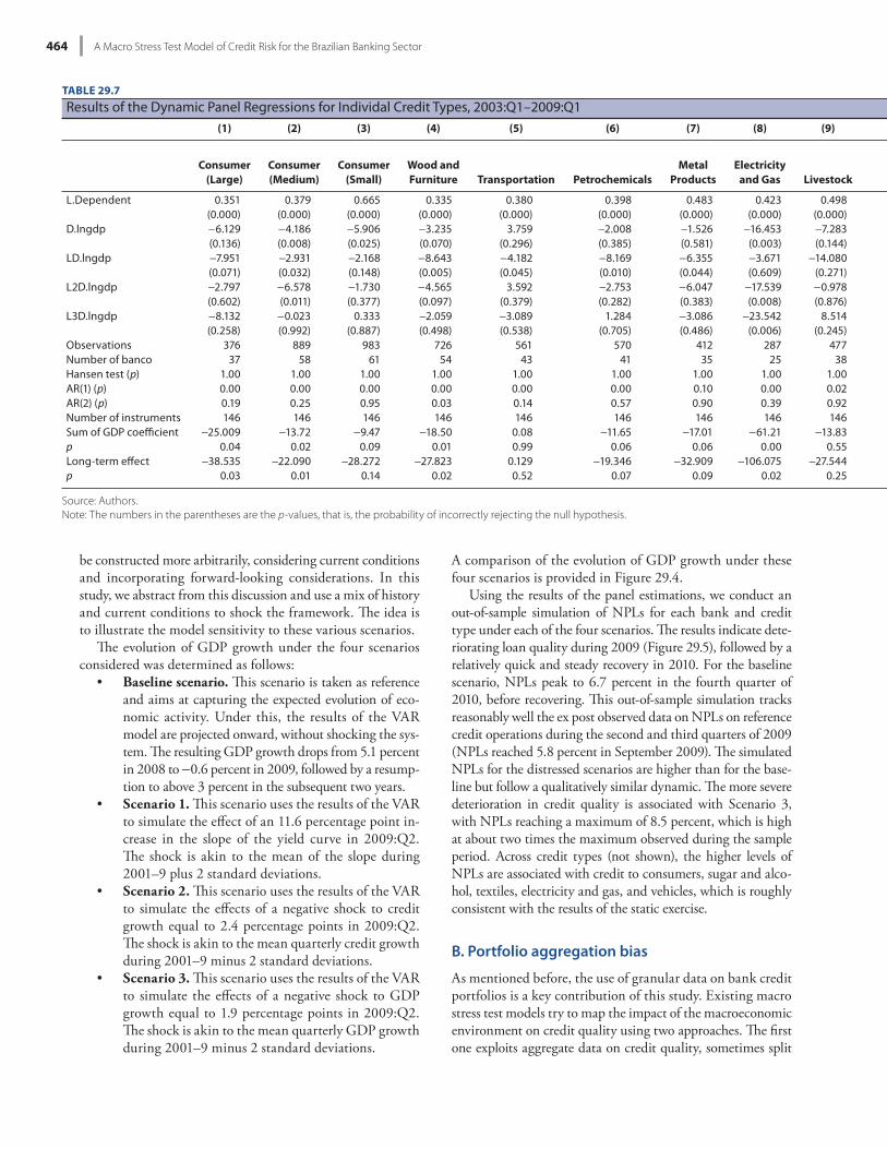
TABLE 29.7

Results of the Dynamic Panel Regressions for Individal Credit Types, 2003:Q1– 2009:Q1(1) (2) (3) (4) (5) (6) (7) (8) (9)

Consumer (Large)

Consumer (Medium)

Consumer (Small)

Wood and Furniture Transportation Petrochemicals

Metal Products

Electricity and Gas Livestock

L.Dependent 0.351 0.379 0.665 0.335 0.380 0.398 0.483 0.423 0.498(0.000) (0.000) (0.000) (0.000) (0.000) (0.000) (0.000) (0.000) (0.000)

D.lngdp 6.129 4.186 5.906 3.235 3.759 2.008 1.526 16.453 7.283(0.136) (0.008) (0.025) (0.070) (0.296) (0.385) (0.581) (0.003) (0.144)

LD.lngdp 7.951 2.931 2.168 8.643 4.182 8.169 6.355 3.671 14.080(0.071) (0.032) (0.148) (0.005) (0.045) (0.010) (0.044) (0.609) (0.271)

L2D.lngdp 2.797 6.578 1.730 4.565 3.592 2.753 6.047 17.539 0.978(0.602) (0.011) (0.377) (0.097) (0.379) (0.282) (0.383) (0.008) (0.876)

L3D.lngdp 8.132 0.023 0.333 2.059 3.089 1.284 3.086 23.542 8.514(0.258) (0.992) (0.887) (0.498) (0.538) (0.705) (0.486) (0.006) (0.245)

Observations 376 889 983 726 561 570 412 287 477Number of banco 37 58 61 54 43 41 35 25 38Hansen test (p) 1.00 1.00 1.00 1.00 1.00 1.00 1.00 1.00 1.00AR(1) (p) 0.00 0.00 0.00 0.00 0.00 0.00 0.10 0.00 0.02AR(2) (p) 0.19 0.25 0.95 0.03 0.14 0.57 0.90 0.39 0.92Number of instruments 146 146 146 146 146 146 146 146 146Sum of GDP coeffi cient 25.009 13.72 9.47 18.50 0.08 11.65 17.01 61.21 13.83p 0.04 0.02 0.09 0.01 0.99 0.06 0.06 0.00 0.55Long- term eff ect 38.535 22.090 28.272 27.823 0.129 19.346 32.909 106.075 27.544p 0.03 0.01 0.14 0.02 0.52 0.07 0.09 0.02 0.25

Source: Authors.Note: The numbers in the parentheses are the p-values, that is, the probability of incorrectly rejecting the null hypothesis.

A comparison of the evolution of GDP growth under these four scenarios is provided in Figure 29.4.

Using the results of the panel estimations, we conduct an out- of- sample simulation of NPLs for each bank and credit type under each of the four scenarios. Th e results indicate dete-riorating loan quality during 2009 (Figure 29.5), followed by a relatively quick and steady recovery in 2010. For the baseline scenario, NPLs peak to 6.7 percent in the fourth quarter of 2010, before recovering. Th is out- of- sample simulation tracks reasonably well the ex post observed data on NPLs on reference credit operations during the second and third quarters of 2009 (NPLs reached 5.8 percent in September 2009). Th e simulated NPLs for the distressed scenarios are higher than for the base-line but follow a qualitatively similar dynamic. Th e more severe deterioration in credit quality is associated with Scenario 3, with NPLs reaching a maximum of 8.5 percent, which is high at about two times the maximum observed during the sample period. Across credit types (not shown), the higher levels of NPLs are associated with credit to consumers, sugar and alco-hol, textiles, electricity and gas, and vehicles, which is roughly consistent with the results of the static exercise.

B. Portfolio aggregation bias

As mentioned before, the use of granular data on bank credit portfolios is a key contribution of this study. Existing macro stress test models try to map the impact of the macroeconomic environment on credit quality using two approaches. Th e fi rst one exploits aggregate data on credit quality, sometimes split

be constructed more arbitrarily, considering current conditions and incorporating forward- looking considerations. In this study, we abstract from this discussion and use a mix of history and current conditions to shock the framework. Th e idea is to illustrate the model sensitivity to these various scenarios.

Th e evolution of GDP growth under the four scenarios considered was determined as follows:

• Baseline scenario. Th is scenario is taken as reference and aims at capturing the expected evolution of eco-nomic activity. Under this, the results of the VAR model are projected onward, without shocking the sys-tem. Th e resulting GDP growth drops from 5.1 percent in 2008 to 0.6 percent in 2009, followed by a resump-tion to above 3 percent in the subsequent two years.

• Scenario 1. Th is scenario uses the results of the VAR to simulate the eff ect of an 11.6 percentage point in-crease in the slope of the yield curve in 2009:Q2. Th e shock is akin to the mean of the slope during 2001– 9 plus 2 standard deviations.

• Scenario 2. Th is scenario uses the results of the VAR to simulate the eff ects of a negative shock to credit growth equal to 2.4 percentage points in 2009:Q2. Th e shock is akin to the mean quarterly credit growth during 2001– 9 minus 2 standard deviations.

• Scenario 3. Th is scenario uses the results of the VAR to simulate the eff ects of a negative shock to GDP growth equal to 1.9 percentage points in 2009:Q2. Th e shock is akin to the mean quarterly GDP growth during 2001– 9 minus 2 standard deviations.



To illustrate the bias stemming from the use of insuffi -cient granularity in banks’ credit portfolios, we use the re-sults of the previous section to estimate the bank- specifi c NPLs under two approaches. Th e fi rst one, akin to typical macro stress test models of credit risk, simulates the evolu-tion of bank- level NPLs without exploiting information on specifi c credit types ( joint portfolios), while the second ex-ploits a partition of banks’ credit portfolios in specifi c credit categories (granular portfolios). Th e two approaches share the same estimation techniques and the two- year macroeco-nomic scenarios described earlier.

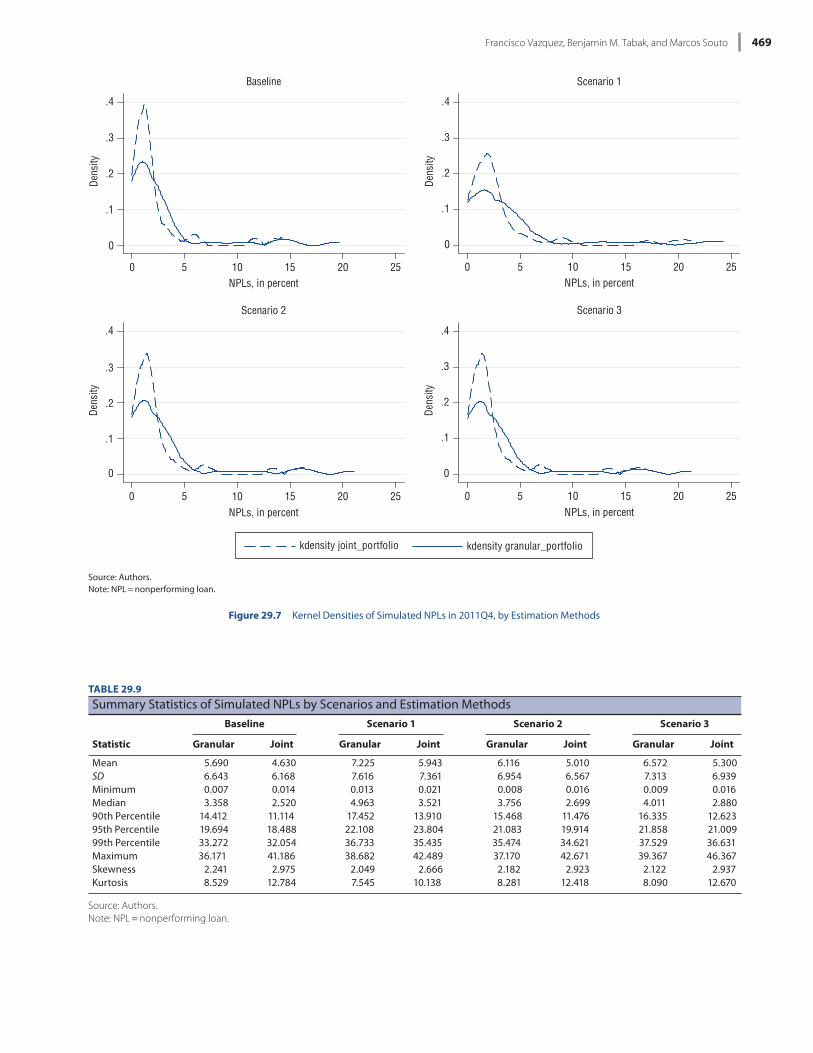
Th e results are consistent with the presence of a bias stem-ming from inadequate granularity in the credit portfolios. In par tic u lar, the weighted average of the simulated NPLs using joint portfolios is always lower than the simulated NPLs un-der the granular portfolios (Figure 29.6). Th e kernel densities of the simulated NPLs under the two approaches also illus-trate this portfolio aggregation bias (Figure 29.7). In par-tic u lar, the mean and the median NPLs under the granular approach exceed those of the joint approach in all cases (Table 29.9). Similarly, the probability mass at the (right) tail of the distributions is also thicker under the granular ap-proach.15 On the other hand, the skewness and kurtosis of the granular approach are lower than those of the joint ap-proach, refl ecting the bias induced by the latter. Paired t- tests

15 Th e maximum value under the granular approach, however, was smaller than the joint approach because of a small bank that started the simula-tion period with very low credit quality.

by economic sectors, and applies econometric techniques to compute (elasticity) pa ram e ters linking macroeconomic con-ditions to credit quality. Th is approach is frequently used to assess systemic fi nancial stability, but it has important short-comings, as the profi les of banks’ credit portfolios and the cushions to absorb credit losses are likely to diff er across banks. Th e validity of the results under this approach becomes weaker as bank sizes, solvency, and risk profi le of their credit portfolios depart from the population mean.

Th e second approach exploits bank- by- bank data on credit quality, albeit without diff erentiating between types of credit and without taking into account information on large expo-sures and other mea sures of portfolio concentration. Although this approach allows the assessment of bank solvency at the level of individual institutions, it has its own shortcomings and po-tential sources of bias. In par tic u lar, the estimated elasticities linking macroeconomic conditions to credit quality refl ect aver-age values, mixing divergent elasticities between types of credit.

Arguably, the latter approach would tend to lead to bi-ased estimations, as the sensitivity of credit quality to mac-roeconomic conditions is likely to diff er between economic sectors. A bank with larger exposures to highly cyclical sec-tors would tend to be more vulnerable to credit losses under an adverse economic scenario. Th erefore, simulations based on this approach would underestimate the potential losses of riskier banks, which is contrary to a prudent principle. In addition, the lack of information on portfolio concentration is a critical shortcoming, as concentration plays a major role in the risk profi le of banks’ credit portfolios.

(10) (11) (12) (13) (14) (15) (16) (17) (18) (19) (20) (21)

Other Ser vices

Sugar and Alcohol

Retail Trade Textile Vehicles Food Agriculture

Health Ser vices Chemicals

Recreation Ser vices

Electrical and Electronic

Equipment Other

0.409 0.340 0.628 0.543 0.522 0.465 0.451 0.443 0.468 0.172 0.352 0.287(0.000) (0.004) (0.000) (0.003) (0.000) (0.000) (0.000) (0.000) (0.000) (0.042) (0.000) (0.000)

2.102 6.134 0.798 0.684 2.170 7.343 11.447 1.207 1.794 3.641 1.032 0.957(0.265) (0.485) (0.722) (0.855) (0.370) (0.005) (0.006) (0.743) (0.442) (0.162) (0.786) (0.769)

3.057 11.806 6.651 10.950 2.901 6.508 11.446 2.730 3.751 5.318 5.744 0.913(0.143) (0.117) (0.004) (0.000) (0.116) (0.032) (0.000) (0.372) (0.188) (0.148) (0.004) (0.704)0.498 24.826 4.095 7.673 1.249 0.124 5.723 2.194 0.632 2.213 1.932 1.008

(0.897) (0.005) (0.239) (0.026) (0.689) (0.971) (0.213) (0.584) (0.863) (0.632) (0.629) (0.854)2.879 24.430 3.719 2.667 5.113 1.821 6.605 2.649 1.060 3.243 9.148 2.825

(0.442) (0.122) (0.189) (0.557) (0.040) (0.628) (0.029) (0.512) (0.670) (0.381) (0.003) (0.450)659 184 502 577 509 549 377 515 443 521 469 711

51 18 41 44 36 42 30 37 39 41 42 511.00 1.00 1.00 1.00 1.00 1.00 1.00 1.00 1.00 1.00 1.00 1.000.00 0.01 0.00 0.00 0.00 0.00 0.00 0.00 0.00 0.01 0.01 0.000.84 0.18 0.11 0.88 0.42 0.35 0.08 0.54 0.85 0.42 0.92 0.82146 144 146 146 146 146 146 146 146 146 146 146

8.54 67.20 15.26 21.97 11.43 15.80 35.22 8.78 3.85 14.42 13.99 3.790.26 0.01 0.01 0.01 0.07 0.03 0.00 0.33 0.43 0.07 0.08 0.69

14.443 101.812 41.030 48.083 23.918 29.525 64.155 15.763 7.242 17.409 21.593 5.3140.18 0.12 0.08 0.26 0.20 0.00 0.00 0.44 0.17 0.17 0.42 0.88



where default rates are assumed to be distributed accord-ing to a gamma distribution, ( k, k ) with k = k

2/ k2 and

k = k2/ k. In turn, k is estimated as k = k/vk, where k is

the expected loss and vk the exposure to credit type k. We use the bank- specifi c estimates of NPLs for each credit type under Scenario 1 as a proxy for distressed PDs. In par tic u lar, we take the average of the out- of- sample simulation of NPLs for each bank and credit type over the fi rst simulated year of Scenario 3 (the more severe) as a proxy for distressed PDs of the corresponding credit categories. To account for uncer-tainty on the true value of the PDs ( k), we use the standard deviation of the NPLs over the corresponding fi rst year of the out- of- sample simulation. Admittedly, NPLs are an im-perfect proxy for PDs because of their “backward- looking” nature. While PDs are intended to capture the likelihood of borrowers’ default within a given horizon (i.e., one year ahead), NPLs typically mea sure the proportion of loans that are more than 90 days past due in total credit portfolios. Th erefore, PDs would vary in response to changes in the repayment capac-ity of a given borrower, which may not immediately translate

of mean diff erences confi rm that the population mean under the granular approach exceeds those resulting from the joint approach in all cases, although diff erences in their population variances are not statistically signifi cant (Table 29.10).

C. Credit VaR

Th is section uses the previous results to compute a credit VaR and come up with an estimate of banks’ (unexpected) credit losses under an adverse macroeconomic environment. For each bank, we model the distribution of credit losses using the CreditRisk+ (Credit Suisse Financial Products, 1997) formula-tion and the exposures of each bank as of March 2009. Under CreditRisk+ and assuming that default probabilities are ran-dom, the probability- generating function G(z) of the normal-ized total expected losses of a portfolio of n credit types can be written as (Avesani and others, 2006)

G(z) = exp1

k2 ln[1 k

2 Pk (z)]k=1

n

, (29.5)

TABLE 29.8

Eff ect of a 2 Percentage Point Drop in GDP Growth on NPLs, by Credit Types (in percent unless indicated)(1) (2) (3) (4) (5) (6) (7) (8) (9) (10)

Estimates of Panel Regressions Increase in NPLs Stressed NPLs

Sector

Average NPLs

2003– 9

NPLs March 2009

Coef. Lagged

NPLs

Sum Coef. GDP

GrowthLong- Term

Eff ectScale

Factor

Short- Term (Percentage

Points)

Long- Term (Percentage

Points) LevelTimes

Increase

Consumer (large) 3.6 2.5 0.4 25.0 38.5 0.035 1.7 2.7 5.2 2.1Consumer (medium) 6.1 5.0 0.4 13.7 22.1 0.057 1.6 2.5 7.6 1.5Consumer (small) 5.9 7.3 0.7 9.5 28.3 0.055 1.0 3.1 10.4 1.4Wood and furniture 3.8 2.8 0.3 18.5 27.8 0.036 1.3 2.0 4.8 1.7Transportation 3.8 1.7 0.4 0.1 0.1 0.037 0.0 0.0 1.7 1.0Petrochemicals 3.6 1.7 0.4 11.6 19.3 0.035 0.8 1.3 3.0 1.8Metal products 2.1 1.0 0.5 17.0 32.9 0.021 0.7 1.4 2.4 2.4Electricity and gas 1.3 0.3 0.4 61.2 106.1 0.013 1.6 2.8 3.1 10.0Livestock 4.2 2.4 0.5 13.8 27.5 0.041 1.1 2.2 4.6 2.0Other ser vices 5.0 3.7 0.4 8.5 14.4 0.047 0.8 1.4 5.1 1.4Sugar and alcohol 0.6 1.3 0.3 67.2 101.8 0.006 0.8 1.2 2.5 1.9Retail trade 3.7 3.0 0.6 15.3 41.0 0.035 1.1 2.9 5.9 2.0Textile 3.9 5.2 0.5 22.0 48.1 0.038 1.7 3.6 8.8 1.7Vehicles 3.0 4.0 0.5 11.4 23.9 0.029 0.7 1.4 5.4 1.3Food 4.3 2.6 0.5 15.8 29.5 0.041 1.3 2.4 5.0 1.9Agriculture 1.7 2.6 0.5 35.2 64.2 0.017 1.2 2.2 4.7 1.8Health ser vices 3.2 2.5 0.4 8.8 15.8 0.031 0.5 1.0 3.5 1.4Chemicals 2.2 2.8 0.5 3.9 7.2 0.021 0.2 0.3 3.1 1.1Recreation ser vices 4.5 4.4 0.2 14.4 17.4 0.043 1.2 1.5 5.9 1.3Electrical equipment 4.9 5.3 0.4 14.0 21.6 0.046 1.3 2.0 7.3 1.4Other 2.9 1.2 0.3 3.8 5.3 0.029 0.2 0.3 0.9 0.7

Overall sampled credit 2.8 3.9 0.6 24.4 60.6 0.027 1.3 3.3 7.2 1.8

Source: Authors.Note: Change in yearly GDP growth:1. Computed as (5) = (4)/(1–(3)).2. The scale factor is computed as: (6) = (1)/(1 – (1)) (i.e., NPL * (1 NPL)).3. Assuming a 2 pp drop in GDP growth, the short- term increase in NPLs is computed as: (7) = (4) * (6) * (– 2).4. The long- term increase in NPLs is computed as: (8) = (7)/(1–(3))5. The stressed PD are computed as: (9) = (2) + (8)Coef. = coeffi cient; NPL = nonperforming loan.



–2

0

2

4

6

2005q3 2007q1 2008q3 2010q1 2011q3

GDP growth, in percent

Baseline Scenario 1 Scenario 2 Scenario 3

Source: Authors.

Figure 29.4 Evolution of GDP Growth under Alternative Scenarios (in percent year- on- year)

0

2

4

6

8

10

2003q1 2006q1 2009q1 2012q1

In percent

Private banks

0

2

4

6

8

10

2003q1 2006q1 2009q1 2012q1

In percent

Public banks

0

2

4

6

8

10

2003q1 2006q1 2009q1 2012q1

In percent

Foreign banks

0

2

4

6

8

10

2003q1 2006q1 2009q1 2012q1

In percent

Total system

Scenario base Scenario 1Scenario 2 Scenario 3

Source: Authors.

Figure 29.5 Evolution of NPLs under Alternative Scenarios



VaR calculation. Moreover, LGDs are likely to vary across credit types, also depending on the existence of collateral on individual credit operations, which we cannot observe. Th ere is also evidence that LGDs tend to vary throughout the cycle, increasing during the economic downturn. Con-versely, to the extent that potential diff erences in the sensi-tivity of LGDs to the economic cycle across credit types go in tandem with the dynamics of their respective PDs, which is likely the case, our relative assessment of individual banks’ solvency would not be biased. Furthermore, our assumption of a 50 percent LGD is likely to be conservative.

Th e pa ram e ters used in the credit VaR are bank specifi c. Although the sensitivities of credit quality to macroeco-nomic conditions are the same for each credit type, the qual-ity of individual banks’ credit portfolios in each of the distressed scenarios would vary according to their starting conditions. Overall, consumer loans and credit to the textile industry, agriculture, and sugar and alcohol are the most procyclical and concentration to the last more pronounced (Table 29.11). Using these pa ram e ters, the distribution of credit losses is computed using the probability- generating function defi ned in equation (29.5), and the unexpected

into changes in NPLs. Using NPLs as a proxy for PDs is prone to various sources of bias that may operate in opposite direc-tions. During the upturn of the economic cycle, which tends to be associated with strong credit growth, NPLs may under-estimate the risk profi le of banks’ credit portfolios. In contrast, NPLs may overestimate credit risk during the downturn, as banks defer loan write- off s.

For each credit type, we conduct an initial calculation of the average exposures to individual borrowers, by dividing the corresponding total exposures over the number of loan operations. Th is treatment, however, may underestimate portfolio concentration and therefore the results of the credit VaR. We thus consider an alternative exercise by assuming that 80 percent of the exposures under each credit category are concentrated in 20 percent of the number of credit op-erations (and the remaining 20 percent of the exposures cor-respond to 80 percent of the number of credit operations). Because we do not have information on losses given default (LGDs), we choose a generic value of 50 percent for all credit types. We recognize that this is also a critical assumption in our assessment of banks’ solvency, as higher LGD would mechanically lead to higher unexpected losses in the credit

2

4

6

8

2003q1 2006q1 2009q1 2012q1

In percent

Baseline

2

4

6

8

2003q1 2006q1 2009q1 2012q1

In percent

Scenario 1

2

4

6

8

2003q1 2006q1 2009q1 2012q1

In percent

Scenario 2

2

4

6

8

2003q1 2006q1 2009q1 2012q1

In percent

Scenario 3

Granular portfolios Joint porfolios


Figure 29.6 Evolution of NPLs by Scenarios and Computation Methods



0

.1

.2

.3

.4De

nsity

0 5 10 15 20 25NPLs, in percent

Baseline

0

.1

.2

.3

.4

Dens

ity


Scenario 1

0

.1

.2

.3

.4

Dens

ity


Scenario 2

0

.1

.2

.3

.4

Dens

ity


Scenario 3

kdensity joint_portfolio kdensity granular_portfolio


Figure 29.7 Kernel Densities of Simulated NPLs in 2011Q4, by Estimation Methods

TABLE 29.9

Summary Statistics of Simulated NPLs by Scenarios and Estimation MethodsBaseline Scenario 1 Scenario 2 Scenario 3

Statistic Granular Joint Granular Joint Granular Joint Granular Joint

Mean 5.690 4.630 7.225 5.943 6.116 5.010 6.572 5.300SD 6.643 6.168 7.616 7.361 6.954 6.567 7.313 6.939Minimum 0.007 0.014 0.013 0.021 0.008 0.016 0.009 0.016Median 3.358 2.520 4.963 3.521 3.756 2.699 4.011 2.88090th Percentile 14.412 11.114 17.452 13.910 15.468 11.476 16.335 12.62395th Percentile 19.694 18.488 22.108 23.804 21.083 19.914 21.858 21.00999th Percentile 33.272 32.054 36.733 35.435 35.474 34.621 37.529 36.631Maximum 36.171 41.186 38.682 42.489 37.170 42.671 39.367 46.367Skewness 2.241 2.975 2.049 2.666 2.182 2.923 2.122 2.937Kurtosis 8.529 12.784 7.545 10.138 8.281 12.418 8.090 12.670




TABLE 29.11

Results of the Credit VaR (in million BRL, unless otherwise indicated)

Bank Number

Credit VaR

Credit VaR/Net

Exposure (Percent)

Credit VaR/

Gross Exposure (Percent)

Gross Exposure

Share of Loans in Sample

(Percent)

1 4,689 5.0 2.5 1,89,052 24.32 11,095 12.8 6.4 1,73,172 22.23 6,865 10.1 5.1 1,35,276 17.44 8,181 14.0 7.0 1,16,957 15.05 1,479 9.3 4.7 31,798 4.16 906 5.8 2.9 31,378 4.07 1,152 10.9 5.5 21,118 2.78 551 11.4 5.7 9,642 1.29 286 6.3 3.2 9,046 1.2

10 347 10.2 5.1 6,839 0.911 20 0.6 0.3 6,348 0.812 506 16.3 8.1 6,216 0.813 185 10.0 5.0 3,675 0.514 161 9.1 4.5 3,538 0.515 200 11.4 5.7 3,502 0.416 71 4.6 2.3 3,113 0.417 309 20.7 10.4 2,985 0.418 116 9.1 4.5 2,563 0.3

Total 37,118 9.8 4.9 7,56,218 97.0

Source: Authors.Notes: Net exposures are computed by subtracting the estimated recov-ery values from the gross credit exposures. Loss given default = 0.5; model = Poisson defaults/fast Fourier transform; VaR = valve at risk. Pa-ram e ters: VaR level = 0.99.

(unexpected) credit losses associated with a 99 percent credit VaR for the 18 banks with the largest credit portfolios in the sample amount to about BRL37 billion, or 4.9 percent of their gross exposures (Table 29.12). As a reference, these losses are roughly equivalent to about 19 percent of the joint tangible capital of these banks. Our mea sure of tangible capital equals regulatory capital minus the sum of specifi c loan loss provi-sions included in banks’ own resources, deferred taxes, and goodwill. Th erefore, the capital cushions of the largest banks appear suffi cient to absorb the credit losses associated with the scenarios considered without threatening fi nancial stability.

4. CONCLUSIONTh e econometric estimations presented in this study provide strong evidence of cyclical behavior of loan quality. Th e estimations substantiate the existence of a robust inverse rela-tionship between GDP growth and NPLs, with the eff ects operating with up to three quarter lags. Th e results also indi-cate diff erences in the per sis tence of NPLs across credit types, and in their sensitivity to economic activity. Loan quality in Brazil appears to be more sensitive to GDP growth for small consumer loans, credit to agriculture, sugar and alcohol, live-stock, and textiles. In addition, credit for vehicle acquisition and electric and electronic equipment displayed a high level of NPLs under distressed macroeconomic scenarios. Banks with relatively higher exposures to these sectors are likely to expe-rience larger credit losses under a macroeconomic downturn.

Although intuitive, the modeling of diff erences in the sensi-tivity of loan quality to macroeconomic conditions at the level of individual banks is novel to the macro stress testing litera-ture. Existing models based on bank- level data do not allow for a diff erential response of credit quality to macroeconomic conditions across credit types, possibly owing to lack of data availability. Conversely, existing macro stress test models that exploit variations in the sensitivity of loan quality to macro-

losses are estimated as the 99th percentile of the expected losses distribution.

Th e results suggest that the banking sector is well prepared to undergo the credit losses associated with the distressed sce-narios considered without threatening fi nancial stability. Th e

TABLE 29.10

Comparison of Simulated Distributions of NPLsTest Baseline Scenario 1 Scenario 2 Scenario 3

Mean paired t- test

(1) Granular (Mean) 5.690 7.225 6.116 6.572(2) Joint (Mean) 4.630 5.943 5.010 5.300Diff erence (1)–(2) 1.060 1.282 1.105 1.273H1: Mean Diff <0 (p) 1.000 1.000 1.000 1.000H1: Mean Diff ~0 (p) 0.000 0.000 0.000 0.000H1: Mean Diff >0 (p) 0.000 0.000 0.000 0.000

Variance ratio test

(1) Granular (SD) 6.643 7.616 6.954 7.313(2) Joint (SD) 6.168 7.361 6.567 6.939Diff erence (1)–(2) 0.475 0.254 0.387 0.374H1: Mean Diff <0 (p) 0.933 0.754 0.876 0.856H1: Mean Diff ~0 (p) 0.134 0.493 0.247 0.288H1: Mean Diff >0 (p) 0.067 0.246 0.124 0.144

Source: Authors.Note: Diff = diff erence; NPL = nonperforming loan.



economic conditions across credit types are based on aggre-gated data, and are therefore less suited to assess the adequacy of bank capital at the level of individual institutions.

Th e results presented in this study show that the lack of suf-fi ciently granular data on the composition of bank credit port-folios can bias the results in a way that is contrary to a prudent criterion. To the extent that the sensitivity of credit quality to macroeconomic conditions varies between diff erent credit types, the lack of diff erentiation would tend to underestimate the deterioration of credit quality for the highly procyclical credit types and sectors under a distressed macroeconomic en-vironment (and overestimate the deterioration of credit quality for the relatively safer credit types). Th ese biases would trans-late in a systematic way into the assessment of bank risk pro-fi les, leading to an underestimation of tail losses in the more vulnerable institutions in the banking system under analysis.

Th e model presented in this study represents an improve-ment over existing literature but is still subject to several im-portant caveats. First, the model assumes a linear relationship between loan quality and macroeconomic conditions, which may fail to capture potential nonlinear relationships during periods of severe macroeconomic distress. Second, the model assumes that historic correlations between loan quality and macroeconomic conditions are symmetric during the upturn and the downturn of the economic cycle and remain valid during periods of severe distress. Th ird, the model fails to capture potential feedback eff ects between credit quality and economic growth, as it does not fully integrate the macro and microeconomic modules. In par tic u lar, the macroeconomic

module allows credit volumes to vary over time, while the microeconomic module assumes that individual banks main-tain constant credit portfolios. To the extent that credit qual-ity tends to deteriorate during periods of slow credit growth, the model presented in this study may underestimate banks’ loan losses. All these caveats may likely bias the results in the same direction during periods of fi nancial distress, causing a potential underestimation of bank credit losses. Further anal-ysis is needed to address these shortcomings.

REFERENCESArellano, Manuel, and Stephen Bond, 1991, “Some Tests of Specifi -

cation for Panel Data: Monte Carlo Evidence and an Application to Employment Equations,” Review of Economic Studies, Vol. 58, No. 2, pp. 277– 97.

Avesani, Renzo, Kexue Liu, Alin Mirestean, and Jean Salvati, 2006, “Review and Implementation of Credit Risk Models of the Fi-nancial Sector Assessment Program,” IMF Working Paper 06/134 (Washington: International Monetary Fund). Available via the Internet: http:// www .imf .org /external /pubs /cat /longres .aspx ?sk =19111

Barnhill, Th eodore, Marcos R. Souto, and Benjamin M. Tabak, 2006, “An Analysis of Off - Site Supervision of Banks’ Profi t-ability, Risk and Capital Adequacy: A Portfolio Simulation Approach Applied to Brazilian Banks,” Working Paper No. 117 (Brasilia: Central Bank of Brazil). Available via the Internet: http:// www .bcb .gov .br /pec /wps /port /wp117 .asp ?idiom=I

Berkowitz, Jeremy, 1999, “A Coherent Framework for Stress- Testing,” Working Paper No. 29, Finance and Economics Discussion Series (Washington: Board of Governors of the Federal Reserve

TABLE 29.12

Credit Risk Pa ram e ters Used to Estimate Credit VaRDistressed PDs Credit Exposures

Sector Mean Median MaxAverage Size (Million BRL)

Number of Operations

Average Credit (Million BRL)

Agriculture 0.14 0.09 0.86 915 1,802 0.508Food 0.03 0.02 0.11 999 4,344 0.230Livestock 0.09 0.03 0.69 1,360 2,513 0.541Vehicles 0.06 0.05 0.21 1,185 7,728 0.153Electrical and electronic equipment 0.11 0.06 0.51 624 4,944 0.126Electricity and gas 0.03 0.00 0.44 1,376 175 7.867Wood and furniture 0.05 0.05 0.12 3,369 17,700 0.190Recreation ser vices 0.04 0.03 0.09 742 9,708 0.076Other 0.02 0.01 0.17 3,755 7,098 0.529Petrochemicals 0.09 0.04 0.42 1,559 4,121 0.378Consumer (large) 0.07 0.04 0.29 1,103 1,782 0.619Consumer (medium) 0.11 0.12 0.22 4,114 66,188 0.062Consumer (small) 0.10 0.09 0.23 10,814 814,219 0.013Chemicals 0.02 0.01 0.07 701 3,760 0.187Health ser vices 0.05 0.04 0.20 809 5,741 0.141Other ser vices 0.07 0.05 0.29 1,318 11,036 0.119Metal products 0.03 0.02 0.17 1,421 1,770 0.803Sugar and alcohol 0.22 0.20 0.77 1,351 172 7.860Textile 0.18 0.13 0.67 1,184 12,264 0.097Transportation 0.02 0.02 0.08 2,173 7,222 0.301Retail trade 0.10 0.05 0.81 1,213 11,631 0.104

Source: Authors.Note: PD = probability of default; VaR = valve at risk.



Pesola, Jarmo, 2001, “Th e Role of Macroeconomic Shocks in Bank-ing Crises,” Discussion Paper 6/2001 (Helsinki: Bank of Fin-land). Available via the Internet: http:// www .suomenpankki .fi /en /julkaisut /tutkimukset /keskustelualoitteet /Pages /dp2001 _6 .aspx ?hl=Th e %20Role %20of %20Macroeconomic %20Shocks %20in %20Banking %20Crises

———, 2005, “Banking Fragility and Distress: An Economic Study of Macroeconomic Determinants,” Discussion Paper 13/2005 (Helsinki: Bank of Finland). Available via the Internet: http:// www .suomenpankki .fi /en /julkaisut /tutkimukset /keskustelua loitteet /Pages /dp2005 _13 .aspx ?hl=Banking %20Fragility %20and %20Distress %3A %20An %20Economic %20Study %20of %20 Ma croeconomic %20Determinants

Rodriguez, Adolfo, and Carlos Trucharte, 2007, “Loss Coverage and Stress Testing Mortgage Portfolios: A Non- Parametric Approach,” Journal of Financial Stability, Vol. 3, No. 4, pp. 342– 67.

Sorge, Marco, 2004, “Stress- Testing Financial Systems: An Over-view of Current Methodologies,” BIS Working Paper No. 165 (Basel: Bank for International Settlements). Available via the Internet: http:// www .bis .org /publ /work165 .htm

———, and Kimmo Virolainen, 2006, “A Comparative Analysis of Macro Stress- Testing Methodologies with Application to Fin-land,” Journal of Financial Stability, Vol. 2, No. 2, pp. 113– 51.

Staub, Roberta B., Geraldo da Silva e Souza, and Benjamin M. Tabak, 2010, “Evolution of Bank Effi ciency in Brazil: A DEA Approach,” Eu ro pe an Journal of Operational Research, Vol. 202, No. 1, pp. 204– 13.

Tabak, Benjamin M., Dimas M. Fazio, and Daniel O. Cajueiro, 2011, “Th e Eff ects of Loan Portfolio Concentration on Brazilian Banks’ Return and Risk,” Journal of Banking and Finance, Vol. 35, No. 11, pp. 3065– 76.

Tabak, Benjamin M., and Roberta B. Staub, 2007. “Assessing Finan-cial Instability: Th e Case of Brazil,” Research in International Business and Finance, Vol. 21, No. 2, pp. 188– 202.

Tecles, Patricia Langsch, and Benjamin M. Tabak, 2010, “Deter-minants of Bank Effi ciency: Th e Case of Brazil,” Eu ro pe an Jour-nal of Operational Research, Vol. 207, No. 3, pp. 1587– 98.

van den End, Jan Willem, Marco Hoeberichts, and Mostafa Tabbae, 2006, “Modelling Scenario Analysis and Macro Stress- Testing,” DNB Working Paper No. 119 (Amsterdam: De Nederlandsche Bank). Available via the Internet: http:// www .dnb .nl /en /publica tions /dnb -publications /dnb -working -papers -series /dnb -working -papers /auto101896 .jsp

Vazquez, Francisco, Benjamin M. Tabak, and Marcos Souto, 2012, “A Macro Stress Test Model of Credit Risk for the Brazilian Banking Sector,” Journal of Financial Stability, Vol. 8, No. 2, pp. 69– 83.

Virolainen, Kimmo, 2004, “Macro Stress Testing with a Macro-economic Credit Risk Model for Finland,” Discussion Paper 18/2004 (Helsinki: Bank of Finland). Available via the Internet: http:// www .suomenpankki .fi /en /julkaisut /tutkimukset /keskust elualoitteet /Pages /dp2004 _18 .aspx ?hl=Macro %20Stress %20 Test ing %20with %20a %20Macroeconomic %20Credit %20Risk %20Model %20for %20Finland

Wilson, Th omas, 1997a, “Portfolio Credit Risk (i),” Risk, Vol. 10, No. 9, pp. 111– 17.

———, 1997b, “Portfolio Credit Risk (ii),” Risk, Vol. 10, No. 10, pp. 56– 61.

Wong, Jim, Ka- fai Choi, and Tom Fong, 2006, “A Framework for Stress Testing Bank’s Credit Risk,” Research Memorandum 15/2006 (Hong Kong SAR: Hong Kong Monetary Authority). Available via the Internet: http:// www .hkma .gov .hk /eng /publi cations -and -research /research /working -papers /pre -2007 .shtml

System). Available via the Internet: http:// www .federalreserve .gov /pubs /feds /1999 /199929 /199929abs .html

Blank, Sven, Claudia M. Buch, and Katja Neugebauer, 2009, “Shocks at Large Banks and Banking Sector Distress: Th e Banking Gran-ular Residual,” Journal of Financial Stability, Vol. 5, No. 4, pp. 353– 73.

Blundell, Richard, and Stephen Bond, 1998, “Initial Conditions and Moment Restrictions in Dynamic Panel Data Models,” Journal of Econometrics, Vol. 87, No. 1, pp. 115– 43.

Boss, Michael, Gerald Krenn, Claus Puhr, and Markus S. Schwaiger, 2007, “Stress Testing the Exposure of Austrian Banks in Central and Eastern Eu rope,” Financial Stability Report, No. 13, pp. 115– 34.

Cardarelli, Roberto, Selim Elekdag, and Subir Lall, 2011, “Financial Stress and Economic Contractions,” Journal of Financial Stabil-ity, Vol. 7, No. 2, pp. 78– 97.

Castrén, Olli, Stéphane Dées, and Fadi Zaher, 2010, “Stress- Testing Euro Area Corporate Default Probabilities Using a Global Macro-economic Model,” Journal of Financial Stability, Vol. 6, No. 2, pp. 64– 78.

Coffi net, Jérôme, and Surong Lin, 2010, “Stress Testing Banks’ Prof-itability: Th e Case of French Banks,” Working Paper No. 306 (Paris: Banque de France). Available via the Internet: http:// www .banque -france .fr /en /economics -statistics /research /working -paper -series /document /306 -1 .html

Coffi net, Jérôme, and Clément Martin, 2009, “Stress Testing French Banks’ Income Subcomponents,” Working Paper No. 242 (Paris: Banque de France). Available via the Internet: http:// www .banque -france .fr /en /economics -statistics /research /working -paper -series /document /242 -1 .html

Credit Suisse Financial Products, 1997, “CreditRisk+: A Credit Risk Management Framework,” Technical Report (London: Credit Suisse First Boston). Available via the Internet: http:// www .csfb .com /institutional /research /assets /creditrisk .pdf

Duellmann, Klaus, and Martin Erdelmeier, 2009, “Crash Testing German Banks,” International Journal of Central Banking, Vol. 5, No. 3, pp. 139– 79.

Foglia, Antonella, 2009, “Stress Testing Credit Risk: A Survey of Authorities’ Approaches,” International Journal of Central Bank-ing, Vol. 5, No. 3, pp. 9– 45.

Frøyland, Espen, and Kai Larsen, 2002, “How Vulnerable Are Finan-cial Institutions to Macroeconomic Changes? An Analysis Based on Stress Testing,” Economic Bulletin, Vol. 3, No. 11, pp. 127– 69.

Gerlach, Stefan, Wensheng Peng, and Chang Shu, 2004, “Macro-economic Conditions and Banking Per for mance in Hong Kong: A Panel Study,” Working Paper (Hong Kong SAR: Hong Kong Monetary Authority). Available via the Internet: http:// www .hkma .gov .hk /eng /publications -and -research /research /working -papers /pre -2007 .shtml

Hoggarth, Glenn, and John Whitley, 2003, “Assessing the Strength of U.K. Banks through Macroeconomic Stress Tests,” Financial Stability Review, No. 14 (London: Bank of En gland). Available via the Internet: http:// www .bankofengland .co .uk /publications /Pages /fsr /2003 /fsr14 .aspx

Illing, Mark, and Ying Liu, 2006, “Mea sur ing Financial Stress in a Developed Country: An Application to Canada,” Journal of Financial Stability, Vol. 2, No. 3, pp. 243– 65.

Misina, Miroslav, and David Tessier, 2008, “Non- Linearities, Model Uncertainty and Macro Stress Testing,” Working Paper 2008- 30 (Ottawa: Bank of Canada). Available via the Internet: http:// www .bankofcanada .ca /2008 /09 /publications /research /working -paper -2008 -30 /


a macro stress test model of credit risk for the brazilian ... · test of credit risk for the...

Documents