a mapping tool for climatological applications

METEOROLOGICAL APPLICATIONSMeteorol. Appl. 18: 230–237 (2011)Published online 17 September 2010 in Wiley Online Library(wileyonlinelibrary.com) DOI: 10.1002/met.233

A mapping tool for climatological applications

Olaf Matuschek and Andreas Matzarakis*Meteorological Institute, Albert-Ludwigs-University Freiburg, Freiburg, Germany

ABSTRACT: Modern GIS tools are inclined to be complex and not well suited to climatological applications. To redressthis situation, a free tool for the creation of maps at different spatial resolutions for biometeorological and climatologicalpurposes has been developed for use by GIS users and non-specialists alike. The method produces grids and isolines onmaps at the same time using a climate mapping tool (CMT), which employs two different algorithms for deriving isolinesfrom gridded data. CMT allows the creation and mapping based on ASCII and CSV files as well as the import of the mostcommon GIS data file formats. The algorithms and the mapping tool developed can be used for a variety of applications,such as mapping of bioclimate indices. A case study using physiologically equivalent temperature (PET) is presented todemonstrate the features of CMT. Copyright 2010 Royal Meteorological Society

KEY WORDS climate mapping tool; isolines; grid data; bioclimate; physiologically equivalent temperature

Received 15 June 2009; Revised 16 April 2010; Accepted 21 July 2010

1. Introduction

Construction of climatological and biometeorologicalmaps is frequently required in climate research(Unkasevic and Radinovic, 2000; Daly et al. 2002; Chap-man and Thornes, 2003; Matzarakis et al., 2007a, 2007b).The tools required for this are particularly relevant to bothclimate change studies and simple climate mapping tasks(Matzarakis et al., 1998; Daly et al. 2002). Traditionalmapping techniques are usually based on the interpolationof point data (usually from meteorological and climato-logical networks) in space (Saurer und Behr, 1997; ESRI,2005; Neteler and Mitasova, 2008). Nowadays, there isa demand for interpolation and mapping of output fromclimate models (Jacob et al., 2001; Zebish et al., 2005;Wunram, 2005; Bohm et al., 2006; Will et al., 2006).Data from regional climate model simulations cover arange of spatial resolutions (from 10 km to more than200 km). In order to visualize such data in meaning-ful ways, several options have to be provided to users.Moreover, it is often necessary to blend together two ormore types of information (Saurer and Behr, 1997). Exist-ing Geographical Information System (GIS) methods andsoftware packages offer such possibilities (Chapman andThornes 2003; ESRI, 2005; Haberman, 2005; Shipley,2005; Neteler and Mitasova, 2008). However, for manytypes of climatological studies, the routines in these pack-ages are too complex. Consequently, the process is diffi-cult and time consuming.

GIS information is often comprised of spatial databasesthat represent aspects of the cultural and physical environ-ment of a particular geographic region. GIS applications

* Correspondence to: Andreas Matzarakis, Meteorological Institute,Albert-Ludwigs-University Freiburg, Werthmannsr. 10, D-79085Freiburg, Germany. E-mail: [email protected]

are used to generate graphical and statistical productsfrom these databases (Saurer and Behr, 1997; Bill, 1999).A typical GIS, therefore, consists of three modules: datainput, data management and visual or statistical output.To visualize different types of information, usually oneor more layers of information can be superimposed. Forclimatological mapping, it is convenient to allow for atleast two layers, such as elevation and the relevant cli-mate parameter or variable. With this in mind, the aimof the current work is to develop an easy to use tool thatcombines the three steps of data input, data managementand visualization into one single step and, at the sametime, provide a visualization of two or more layers ofinformation (Matzarakis et al., 2007b).

The paper is organized as follows. First, relevant mete-orological applications are reviewed. Next, developmentof the climate mapping tool is described, followed by adescription of the development of algorithms for the cre-ation of isolines. Finally, a case study is presented, whichinvolves the creation of a maps of the biometeorologicalthermal index Physiologically Equivalent Temperature(PET). The PET index describes the effect of climateon the human organism based on future regional climatescenarios runs for Europe.

2. Methods

The focus of the method presented here is to develop auser friendly tool for the generation of meteorological orclimatological maps. Although these maps can be createdusing a standard GIS package, they are expensive andrequire specialized knowledge and considerable time tocomplete the mapping task. The aim here is to producea user friendly, easy-to-use mapping tool that is freelyavailable via the Web, for example along the lines

Copyright 2010 Royal Meteorological Society

A mapping tool for climatological applications 231

provided by ‘RayMan’ (Matzarakis et al., 2007c). As theprogramming language used is C#, calculation routinescan be run on any standard Microsoft Windows-basedcomputer.

The approach allows data of different formats andstructures to be read (imported) and then processed so asto produce maps using a variety of different visualizationtechniques. The user is given different options, but ineach case gridded and isoline output can be mapped atthe same time. The technique developed to draw isolinesis one of the most challenging yet important features ofthis tool. Details are presented in Section 2.3.

2.1. Existing meteorological applications

Existing meteorological visualization mapping applica-tions include ArcGIS (ESRI, 2005), GRASS and GrADS.These are all complex software packages that can beused via Windows (ArcGIS, GRASS) or Linux (GRASS,GrADS) operating systems. While ArcGIS has a graph-ical user interface, the latter two software packages arelargely operated through the command line or a scriptinginterface. All three software packages require the userto have acquired considerable experience with the soft-ware and its procedures and are several steps away froma ‘switch-on-and-use’ mapping product.

Meteorological and climatological data for modellingare typically processed in tab-delimited text format, oras comma separated values (CSV) (Matzarakis et al.,2007c). Each line contains the latitude, longitude andheight, as well as other relevant parameters such asair temperature and water vapour pressure. These textformats have the advantage of being ‘human readable’.They can be easily processed by a variety of standard

software tools such as Microsoft Excel or the SPSSstatistics package. Working with text files is possiblewith all three above mentioned visualization packages,though certain limitations apply. ArcGIS has a text importfilter that allows the user to convert specially preparedtext files to ‘point-shape’ files. With further processingsteps, these shape files can be converted and visualizedas raster grids, or in any of the various options providedby ArcGIS. Similar text-import filters exist in Excel andSPSS packages as well. The steps for use involve firstimporting several text files (for example, one with thespecial distribution of mean air temperature, and onewith the calculated PET), then further pre-processingsteps in which the user is able to visualize the outputfor comparison (for example, by presenting one airtemperature as raster, and PET on top as isolines).

Although visualization of biometeorological or climatemodel data is possible using any of the three softwarepackages mentioned above, acquiring the software iscostly and using it is quite involved.

2.2. Climate mapping tool

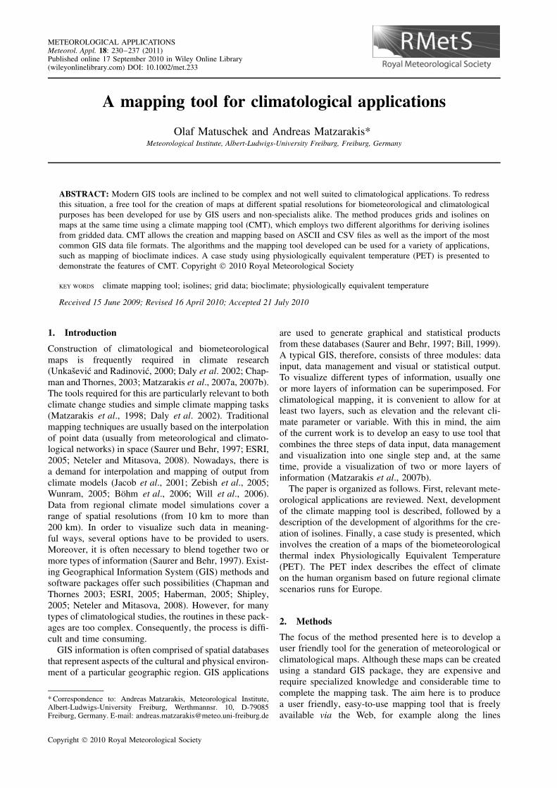
The climate mapping tool (CMT) generates maps frommeteorological and climatological grid data. CMT allowsthe visualization of several data sets by overlaying multi-ple layers. In the lower layer grid, data can be visualizedby defining a colour gradient. In the overlaid layers iso-lines can be drawn using the algorithms described below.Figure 1 shows a screenshot of the program displayingthe topography of the Black Forest in southwest Ger-many. A legend is included on the right hand side.

A typical workflow with CMT is as follows (Figure 1).First, the desired dataset is loaded by clicking on ‘Add

Figure 1. ‘Climate Mapping Tool’ software. This figure is available in colour online at wileyonlinelibrary.com/journal/met

Copyright 2010 Royal Meteorological Society Meteorol. Appl. 18: 230–237 (2011)

232 O. Matuschek and A. Matzarakis

Data Source’ and selecting the appropriate file. Raster fileformats that are supported include CSV and ASCII data,produced with Excel or SPSS, or, for example, ‘RayMan’(Matzarakis et al., 2007c). CMT includes an algorithmto detect encoding, column separator and number formatof these files automatically, so that the time consumingstep of manually entering these values found in mostother software packages is not necessary. Furthermore,CMT automatically detects the structure of rows andcolumns of CSV and ASCII files. Other file formatsthat are supported include GeoTIFF and several formatsproduced by output from weather forecast and climatemodels, though certain restrictions apply. GIS data suchas rivers or state boundaries can be loaded as well, to givea more detailed or realistic picture of the geographicalstructures. Typical GIS file formats such as shape filesand E00 files are supported. After selecting the data, theresults will show up in the data layer list on the upperright side of Figure 1.

The second step is to configure the visualization. Thisincludes selecting certain data from the data source to bevisualized, which can be the column in CSV files, or thetime step found in GRIB files. The type of visualization isselected through ‘Display Mode’, which for grid data canbe as raster through a colour gradient or as a collectionof isolines. The third step is to configure map generationoptions, including generation of map title, ticks and northarrow. If selected, map ticks are drawn automaticallyat logical positions. A specially developed algorithmcalculates this position, so that the step of entering tickposition manually found in most other GIS is no longernecessary. In addition, geographical projections can beapplied in order to produce more realistic maps for theuser. The last step consists of the generation of the mapby selecting the ‘Generate’ button. The maps can besaved in PNG or JPG format and printed by any graphicssoftware.

2.3. Raster and vector concepts

Spatial data in GIS are represented either as grid or asvector data (Saurer and Behr, 1997). A raster divides anarea in elements (cells) of specific size, usually in squaresor rectangles. Each cell can be addressed with its uniquecoordinate X/Y. A cell contains information such as totalprecipitation amount or mean annual air temperature ata specific height, usually at 2 m above sea level. Thisinformation, the value of the cell, can be continuous ordiscrete. For example, precipitation would be continuous,but climate classification would be discrete. Grid pointsrepresent a similar concept, but differ from grid cellsinsofar as here its value is associated with the point onthe edges, not with the area of the cell.

Gridded (raster) data are best used for spatially con-tinuous data. On the other hand, vector data are mostsuitable for spatially discrete data, such as the location ofcities, the run of a river, or the borders and area of a coun-try. Vector data can also be used to represent spatiallycontinuous data, for example through triangular irregular

nets or isolines. Isolines can be seen as a different rep-resentation of the same underlying information as rasterdata. Both representations can, therefore, be transformedinto each other.

2.4. Deriving isolines from raster data

Isolines are represented in a GIS as multiple vectorizedlines. Each line connects points with the same nominalvalue, e.g. 20 °C. Both algorithms developed here workon the basis of deriving each isoline independently oneafter the other. Therefore, only the creation of a singleisoline is discussed below.

The first algorithm developed, the point connectingalgorithm, (a) first finds all raster cells that belong toan isoline, and, (b) connects these cells to an isoline.Detecting raster cells is done by checking the four cornersof each cell. If there are values higher and lower than thevalue of the isoline, it will certainly cross this cell.

Figure 2 shows the basics of this algorithm. Each lineis scanned for line segments, that is points lying nextto each other (Figure 2(a)). All segments identified areconnected to segments on the previous line (Figure 2(b)).Depending on location of start points and end points, asegment might have to be swapped when connected. InFigure 2(e), the segment 10-11-12 has to be connectedas 12-11-10 to point 8. Finally, partial isolines have tobe checked and closed if appropriate (Figure 2(f)). Thereis a couple of special cases to consider when connectingthe points. One such case is shown in Figure 3. Afterconnecting the points 35 and 36 in Figure 3(a), the nextstep with the algorithm described above would be toconnect the segment 41-40-39-38 to point 35. After this,a connection to point 36 is not possible. Such potentiallyambiguous cases are detected by checking all partitionedisolines after the processing of each row, if their start andendpoint are on the same row. If this is not the case, thelast added segments are checked if they can be broken upto satisfy this condition (Figure 3(c)). A few other specialcases may exist with segments consisting of only one, twoor three points, where segments have to be broken up aswell (see Figure 3(c), point 37).

The second algorithm for deriving isolines, the edgeinterpolation algorithm, is based on Snyder (1978), whopresents an algorithm to output isolines derived froma raster on a plotter. While this algorithm as a wholeis not suitable for the problem, its determination ofisoline segment proves most useful. To find parts ofan isoline, four adjoining raster points representing arectangle are evaluated at a time. Each grid edge is thentested for an intersection with an isoline through linearinterpolation. Three cases have to be distinguished: (1) nointersections, no isoline segments, (2) two intersections,the two intersecting points are connected with an isolinesegment, and, (3) four intersections, depending on thelocation on the intersection points on the upper and loweredge two isoline segments are connected. After findingthe segments going through each cell, they can be relativestraightforwardly connected to isolines: segments that



Figure 2. Connection between point and isolines (simple case).

Figure 3. Connection between point and isolines (special cases).

have to be connected share the same point on a gridedge. There are eight ambiguous cases to consider, andthese occur when one or more grid point values equal theisoline value.

During the development of the isoline algorithms, agraphical interface for testing the algorithms was devel-oped. This graphical interface allows for the testing ofthe algorithm row by row by visualizing their output.This immediate visual feedback allowed assessing map-ping problems that might arise at each stage.

3. Results with examples

A variety of possible options is presented by (a) by test-ing and comparing the two different kinds of algorithmsfor isolines drawn (identified), and, (b) the application

and visualization of a thermal index (PET) for the assess-ment of the thermal environment of humans based onresults of regional climate models for the IPCC futureclimate scenario A1B.

3.1. Comparison of algorithms

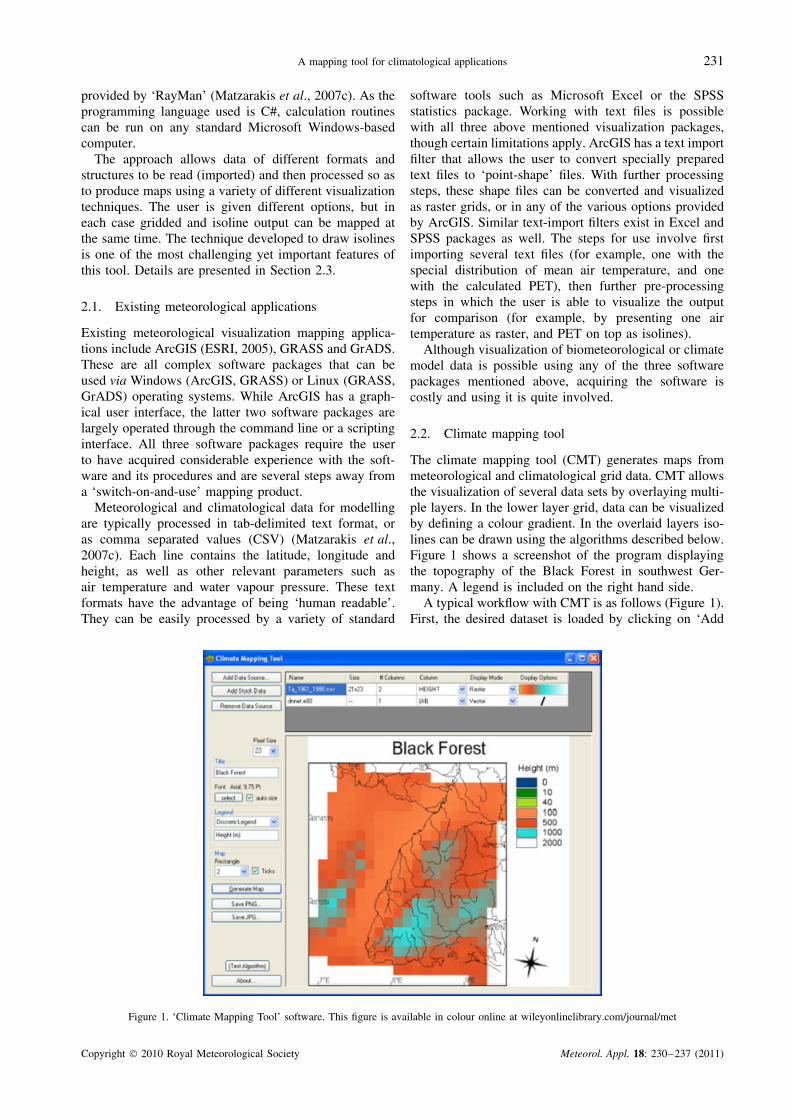
The comparison of the algorithms used is shown inFigure 4. The study area in this case is the German NorthSea coast. The cells contain the number of days per yearwith temperature >20 °C for a specific period and the35 day isoline calculated. Cells with a black backgroundhave been detected by the first algorithm step (a) tobelong to an isoline. Cells with a grey background arenot to be crossed by an isoline, as determined by thisalgorithm. Cells in white are those with no data.



Point connecting algorithm, with smoothing

Edge interpolating algorithm, no smoothing

(a)

(b)

Figure 4. Comparison of algorithms for the creation of isolines.

Both algorithms successfully connect all highlightedraster cells. Algorithm (a) is successful in connecting allspecial cases in the upper right corner: however, iso-lines always go through the middle of each cell. Despitesmoothing (Armstrong, 2005), it appears blocky. Iso-lines generated by algorithm (b) run through interpolatedpoints and seem to be more exact.

In the upper right corner both algorithms generate iso-lines of a different shape. Again algorithm (b) generatesmore accurate results, since it can operate on more infor-mation: it does not connect contextless points as algo-rithm (a), but premade parts of an isoline.

3.2. Comparison of overlay techniques andinterpolation considerations

There are three important techniques for combining twoor more climate/meteorological parameters on one mapfor visual comparison. These are mapematics (i.e. mapalgebra), transparency and isolines. Mapematics is animportant methodology for combining raster data byapplying an algebraic formula to cell values from two ormore layers (ESRI, 2005). Its application is best suited totask where in-depth data analysis is required. Mapematicsrequire exact knowledge of the calculation process anddata interpretation. CMT is intended to be a simplegeneration tool for climate and climate modelling data inraster formats. Therefore, mapematics are not included.Algebraic calculations on the input data can be performedbefore using CMT. Transparency has not been integratedinto CMT in favour of isolines, which seems to be themost straightforward way to overlay two types of data.

An often requested feature for CMT is the gener-ation of maps from irregularly spaced locations, e.g.weather stations. While this would allow for easy visu-alization of measured meteorological parameters, a fewtheoretical problems arise. Drawing maps from irregu-lar spaced locations requires spatial interpolation betweenthese locations. There is no general algorithm to trans-fer point information to space for any meteorologi-cal/climatological parameter (Mesquita and Sousa, 2009).Different approaches and limitations exist for the differ-ent meteorological parameters, and for different regionsof the world (Mesquita and Sousa, 2009). For air tem-perature, for example, a digital elevation model (DEM)at least has to be considered.

3.3. Application of CMT for PET mapping

In this section a regional climate scenario run based onthe CLM – model (Wunram, 2005; Bohm et al., 2006;Will et al., 2006) is used. The daily data from theA1B scenario are used for the periods 1991–2000 and2091–2100, and calculated PET based on VDI (1998),Hoppe (1999) and Matzarakis et al. (1999), in order toquantify the human thermal bioclimate for the wholeof Europe. PET builds a valuable method in order toquantify the effect of the thermal environment on humansbased on the energy exchange of the human body andquantifies the heat effects, i.e. heat stress conditions(Hoppe, 1999). The calculation of PET is produced bythe RayMan model (Matzarakis et al., 2007c). Daily datafrom CLM (air temperature, air humidity, wind speed,global radiation, albedo and Bowen’s ratio) have beenimported into the RayMan and PET calculation routines



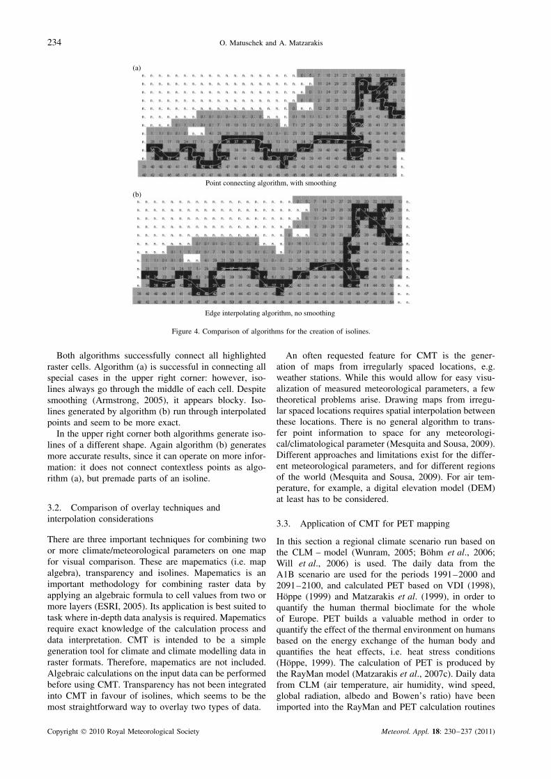
for standard PET thermophysiological conditions (VDI,1998). From the PET results the PET >35 °C days hasbeen accounted and used as import values for CMT-mapping.

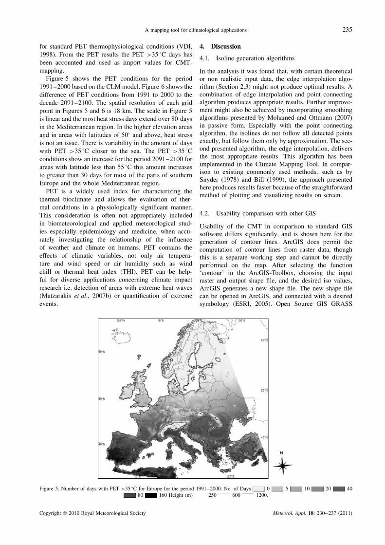
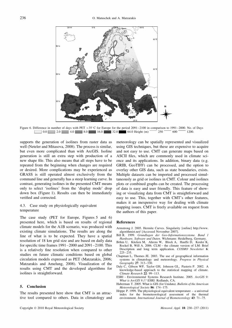
Figure 5 shows the PET conditions for the period1991–2000 based on the CLM model. Figure 6 shows thedifference of PET conditions from 1991 to 2000 to thedecade 2091–2100. The spatial resolution of each gridpoint in Figures 5 and 6 is 18 km. The scale in Figure 5is linear and the most heat stress days extend over 80 daysin the Mediterranean region. In the higher elevation areasand in areas with latitudes of 50° and above, heat stressis not an issue. There is variability in the amount of dayswith PET >35 °C closer to the sea. The PET >35 °Cconditions show an increase for the period 2091–2100 forareas with latitude less than 55 °C this amount increasesto greater than 30 days for most of the parts of southernEurope and the whole Mediterranean region.

PET is a widely used index for characterizing thethermal bioclimate and allows the evaluation of ther-mal conditions in a physiologically significant manner.This consideration is often not appropriately includedin biometeorological and applied meteorological stud-ies especially epidemiology and medicine, when accu-rately investigating the relationship of the influenceof weather and climate on humans. PET contains theeffects of climatic variables, not only air tempera-ture and wind speed or air humidity such as windchill or thermal heat index (THI). PET can be help-ful for diverse applications concerning climate impactresearch i.e. detection of areas with extreme heat waves(Matzarakis et al., 2007b) or quantification of extremeevents.

4. Discussion

4.1. Isoline generation algorithms

In the analysis it was found that, with certain theoreticalor non realistic input data, the edge interpolation algo-rithm (Section 2.3) might not produce optimal results. Acombination of edge interpolation and point connectingalgorithm produces appropriate results. Further improve-ment might also be achieved by incorporating smoothingalgorithms presented by Mohamed and Ottmann (2007)in passive form. Especially with the point connectingalgorithm, the isolines do not follow all detected pointsexactly, but follow them only by approximation. The sec-ond presented algorithm, the edge interpolation, deliversthe most appropriate results. This algorithm has beenimplemented in the Climate Mapping Tool. In compar-ison to existing commonly used methods, such as bySnyder (1978) and Bill (1999), the approach presentedhere produces results faster because of the straightforwardmethod of plotting and visualizing results on screen.

4.2. Usability comparison with other GIS

Usability of the CMT in comparison to standard GISsoftware differs significantly, and is shown here for thegeneration of contour lines. ArcGIS does permit thecomputation of contour lines from raster data, thoughthis is a separate working step and cannot be directlyperformed on the map. After selecting the function‘contour’ in the ArcGIS-Toolbox, choosing the inputraster and output shape file, and the desired iso values,ArcGIS generates a new shape file. The new shape filecan be opened in ArcGIS, and connected with a desiredsymbology (ESRI, 2005). Open Source GIS GRASS

Figure 5. Number of days with PET >35 °C for Europe for the period 1991–2000. No. of Days 0 5 10 20 4080 160 Height (m) 250 600 1200.



Figure 6. Difference in number of days with PET >35 °C for Europe for the period 2091–2100 in comparison to 1991–2000. No. of Days0.0 2.0 4.0 8.0 16.0 32.0 64.0 Height (m) 250 600 1200.

supports the generation of isolines from raster data aswell (Neteler and Mitasova, 2008). The process is similar,but even more complicated than with ArcGIS. Isolinegeneration is still an extra step with production of anew shape file. This also means that all steps have to berepeated from the beginning when changes are requiredor desired. More complications may be experienced asGRASS is still operated almost exclusively from thecommand line and generally has a steep learning curve. Incontrast, generating isolines in the presented CMT meansonly to select ‘isolines’ from the ‘display mode’ dropdown box (Figure 1). Results can then be immediatelyverified and corrected.

4.3. Case study on physiologically equivalenttemperature

The case study (PET for Europe, Figures 5 and 6)presented here, which is based on results of regionalclimate models for the A1B scenario, was produced withexisting climate simulations. The results are along theline of what is to be expected. They have a spatialresolution of 18 km grid size and are based on daily datafor specific time frames 1991–2000 and 2091–2100. Thisis a relatively fine resolution when compared to otherstudies on future climatic conditions based on globalcirculation models expressed as PET (Matzarakis, 2006;Matzarakis and Amelung, 2008). Visualization of theresults using CMT and the developed algorithms forisolines is straightforward.

5. Conclusion

The results presented here show that CMT is an attrac-tive tool compared to others. Data in climatology and

meteorology can be spatially represented and visualizedusing GIS techniques, but these are expensive to acquireand not easy to use. CMT can generate maps based onASCII files, which are commonly used in climate sci-ence and its applications. In addition, binary data (e.g.GRIB, GeoTIFF) can be processed, and the option tooverlay other GIS data, such as state boundaries, exists.Multiple datasets can be imported and processed simul-taneously as grid or isolines in CMT. Colour and isolinesplots or combined graphs can be created. The processingof data is easy and user friendly. This feature of show-ing or visualizing data from CMT is straightforward andeasy to use. This, together with CMT’s other features,makes it an inexpensive way for dealing with climatemapping issues. CMT is freely available on request fromthe authors of this paper.

ReferencesArmstrong J. 2005. Hermite Curves. Singularity [online] http://www.

algorithmist.net/ [Accessed November 2007].Bill R. 1999. Grundlagen der Geo-Informationssysteme. Band 1

Hardware, Software und Daten. Wichmann: Heidelberg, Germany.Bohm U, Kucken M, Ahrens W, Block A, Hauffe D, Keuler K,

Rockel B, Will A. 2006. CLM – the climate version of LM: BriefDescription and long term application. COSMO Newsletter 6:225–235.

Chapman L, Thornes JE. 2003. The use of geographical informationsystems in climatology and meteorology. Progress in PhysicalGeography 27: 313–330.

Daly C, Gibson WP, Taylor GH, Johnson GL, Pasteris P. 2002. Aknowledge-based approach to the statistical mapping of climate.Climate Research 22: 99–113.

ESRI – Environmental Systems Research Institute. 2005. ArcGIS 9:What is ArcGIS 9.1? ESRI: Redlands, CA.

Haberman T. 2005. What is GIS (for Unidata). Bulletin of the AmericanMeteorological Society 86: 174–175.

Hoppe P. 1999. The physiological equivalent temperature – a universalindex for the biometeorological assessment of the thermalenvironment. International Journal of Biometeorology 43: 71–75.



Jacob D, Andrae U, Elgered G, Fortelius C, Graham LP, Jack-son SD, Karstens U, Koepken Chr, Lindau R, Podzun R, Rockel B,Rubel HB, Sass RND, Smith BJJM, Van den Hurk X, Yang X. 2001.A comprehensive model intercomparison study investigating thewater budget during the BALTEX-PIDCAP period. Meteorology andAtmospheric Physics 77: 19–43.

Matzarakis A. 2006. Weather and climate related information fortourism. Tourism and Hospitality Planning & Development 3:99–115.

Matzarakis A, Amelung B. 2008. Physiologically equivalent tem-perature as indicator for impacts of climate change on ther-mal comfort of humans. In Seasonal Forecasts, Climatic Changeand Human Health, Advances in Global Change Research , Thom-son MC, Garcia-Herrera R, Beniston M (eds), Vol. 30. Springer-Sciences and Business Media: Dordrecht, the Netherlands; 161–172.

Matzarakis A, Balafoutis Ch, Mayer H. 1998. Construction ofbioclimate and climate maps of Greece. Proceedings of the4th Panhellenic Congress Meteorology-Climatology-Physics of theAtmosphere, September 1998, Vol. 3, Athens, Greece; 477–482.

Matzarakis A, de Freitas CR, Scott D. 2007a. Developments in TourismClimatology. ISBN 978-3-00-024110-9. Self publishing: Freiburg,Germany.

Matzarakis A, Koch E, Rudel E. 2007b. Analysis of summer tourismperiod for Austria based on climate variables on daily basis. InDevelopments in Tourism Climatology, Matzarakis A, de Freitas CR,Scott D (eds). 122–128.

Matzarakis A, Mayer H, Iziomon MG. 1999. Application of a universalthermal index: physiological equivalent temperature. InternationalJournal of Biometeorology 43: 76–84.

Matzarakis A, Rutz F, Mayer H. 2007c. Modelling radiation fluxesin simple and complex environments – application of the RayManmodel. International Journal of Biometeorology 51: 323–334.

Mesquita S, Sousa AJ. 2009. Bioclimatic mapping using geostatisticalapproaches: application to mainland Portugal. International Journalof Climatology 29: 2156–2170.

Mohamed KA, Ottmann T. 2007. Active-smoothing in digital inkenvironments. EMME 07: Proceedings of the International Workshopon Educational Multimedia and Multimedia Education, held inSeptember 2007. ACM: Augsburg, Germany; 119–120.

Neteler M, Mitasova H. 2008. Open Source GIS : A GRASS GISApproach, 3rd edn. Springer: New York, NY.

Saurer H, Behr R. 1997. Geographische Informationssysteme. EineEinfuhrung. Wissenschaftliche Buchgesellschaft: Darmstadt, Ger-many.

Shipley ST. 2005. GIS applications in meteorology, or adventures ina parallel universe. Bulletin of the American Meteorological Society86: 171–173.

Snyder WV. 1978. Algorithm 531 – contour plotting [J6]. ACMTransactions on Mathematical Software 4: 290–294.

Unkasevic M, Radinovic D. 2000. Statistical analysis of dailymaximum and monthly precipitation at Belgrade. Theoretical andApplied Climatology 66: 241–249.

VDI. 1998. VDI-Guidelines 3787, Part I: Climate. Part 2: Methods forthe Human-Biometeorological Evaluation of Climate and Air Qualityfor Urban and Regional Planning . Beuth: Berlin; 29 pp.

Will A, Keuler K, Block A. 2006. The climate local model –evaluation results and recent developments. TerraFLOPS Newsletter8: 2–3.

Wunram C. 2005. Regional climate modelling with CLM. TerraFLOPSNewsletter 6: 5–6.

Zebisch M, Grothmann T, Schroter D, Hasse C, Fritsch U, Cramer W.2005. Climate change in Germany - vulnerability and adaptation ofclimate sensitive sectors. Climate Change 10/05. Umweltbundesamt:Dessau, Germany.


a mapping tool for climatological applications

Documents