a mathematical and numerical framework for the … · a mathematical and numerical framework for...

Journal of Computational Physics, Accepted 24 February (2016)

1

A Mathematical and Numerical Framework for the Analysis of Compressible Thermal Convection

in Gases at very high Temperatures Marcello Lappa1

1Department of Mechanical and Aerospace Engineering, University of Strathclyde, James Weir Building, 75 Montrose Street, Glasgow, G1 1XJ, UK – email: [email protected], [email protected] The relevance of non-equilibrium phenomena, nonlinear behavior, gravitational effects and fluid compressibility in a wide range of problems related to high-temperature gas-dynamics, especially in thermal, mechanical and nuclear engineering, calls for a concerted approach using the tools of the kinetic theory of gases, statistical physics, quantum mechanics, thermodynamics and mathematical modeling in synergy with advanced numerical strategies for the solution of the Navier-Stokes equations. The reason behind such a need is that in many instances of relevance in this field one witnesses a departure from canonical models and the resulting inadequacy of standard CFD approaches, especially those traditionally used to deal with thermal (buoyancy) convection problems. Starting from microscopic considerations and typical concepts of molecular dynamics, passing through the Boltzmann equation and its known solutions, we show how it is possible to remove past assumptions and elaborate an algorithm capable of targeting the broadest range of applications. Moving beyond the Boussinesq approximation, the Sutherland law and the principle of energy equipartition, the resulting method allows most of the fluid properties (density, viscosity, thermal conductivity, heat capacity and diffusivity, etc.) to be derived in a rational and natural way while keeping empirical contamination to the minimum. Special attention is deserved as well to the well-known pressure issue. With the application of the socalled multiple pressure variables concept and a projection-like numerical approach, difficulties with such a term in the momentum equation are circumvented by allowing the hydrodynamic pressure to decouple from its thermodynamic counterpart. The final result is a flexible and modular framework that on the one hand is able to account for all the molecule (translational, rotational and vibrational) degrees of freedom and their effective excitation, and on the other hand can guarantee adequate interplay between molecular and macroscopic-level entities and processes. Performances are demonstrated by computing some incompressible and compressible benchmark test cases for thermal (gravitational) convection, which are then extended to the high-temperature regime taking advantage of the newly developed features.

Keywords: Buoyancy Convection, High temperature, Projection method, non-Boussinesq effects,

Molecular degree of freedom excitation

1. Introduction

Variable density flows occurring at low Mach number are encountered in several physical

phenomena. Applications involving such flows abound in the fields of thermal, mechanical,

chemical, civil and nuclear engineering. Many industrial (and also nonindustrial) applications in

heat transfer have directly or indirectly engaged with research in these fields.

As an example, the “natural” motion of gases in enclosures with different aspect ratios is relevant to

various engineering areas such as heat transfer from electronic packaging (Sun and Jaluria [1]),


2

furnace engineering (Baltasar et al. [2]), the production of semiconductor and optoelectronics

materials (where the processing itself requires that the high-temperature melt is in contact with a

gas, e.g., the Bridgman, CZ and Floating Zone methods, Lappa and Savino [3]; Lappa [4] and

references therein).

Low-Mach-number natural flows of compressible gases play a key role in numerous other

technological contexts, such as the cooling of high-power devices, solar energy and nuclear power

plants (von Backström and Gannon [5]; Elmo and Cioni [6]; Hu et al.[7]; Martineau et al. [8]).

Other relevant examples include (but are not limited to) plumes from urban mass fires, the release

in the atmosphere of smokes from industrial stacks (McGrattan et al. [9]), plumes resulting from

nuclear explosions and pyroclastic flows from volcanic eruptions (Valentine and Wohletz [10]).

In spite of considerable research and efforts on such topics, a clear and urgent need does exist to

develop new strategies to attack these problems.

First of all, the vast majority of natural convection calculations that have been reported in the

literature have been performed after invoking the Oberbeck–Boussinesq (OB) approximation (see,

e.g., Lappa [11,12]). This approximation relies on a first-order Taylor series to approximate the

density variations according to the difference between local temperature and a reference

temperature. More precisely, it ignores the temperature dependence of all fluid properties, except

for the temperature-induced density variation that is retained in the buoyant force driving the flow.

This philosophy is highly effective if density variations are low. Nevertheless, neglecting the

importance of density variations in thermal flows of gravitational nature with strong temperature

differences can cause a considerable departure from the correct prediction of fluid flow behavior

(non-Oberbeck–Boussinesq (NOB) effects inevitably arise).

For large temperature differences, the Boussinesq assumption breaks down (Gray and Giorgini [13])

and, in order to capture NOB effects, one needs to resort to a compressible flow model, or since the

Mach number remains small, to a low Mach number approximation model.

2. A review of existing algorithms

As explained in Munz et al. [14] and Beccantini et al. [15], the main difficulty in constructing

numerical methods for low-speed compressible flows is the fact that, in the transition from

compressible to incompressible flows, the governing equations change nature. The popular Euler

equations for compressible flows are hyperbolic in nature, but they become hyperbolic-elliptic as

the characteristic flow speed becomes zero compared with the sound speed (i.e. in the limit as the

Mach number tends to zero).

The strategies elaborated over the years to deal with such a complex issue can be roughly divided

into two main categories: the so-called density-based solvers and the pressure-based methods,

which in turn have given rise to two lines of inquiry running in parallel in the literature.

The first category consists of variants of methods originally conceived to deal with the compressible

Navier-Stokes equations. It is well known that such methods in their original fully-compressible


3

formulation cannot be used to compute flows at low Mach regime without major modification. The

reason is the existence of a large disparity between the eigenvalues of the Euler equations (Turkel

[16]). In the last two decades, different techniques have been developed to extend these solvers to

the quasi-incompressible regime, based on the modification of the time-dependent properties of the

governing equations (to cluster the otherwise poorly distributed eigenvalues of the Euler equations)

or on alternate forms of the related integration strategies (Volpe [17]; Guillard and Viozat [18];

Mary et al. [19]; Paillere et al. [20]; Vierendeels et al. [21]; Parchevsky [22]; Martineau et al. [8];

Könözsy and Drikakis [23]). The resulting solvers often allow the simulation of flows ranging from

supersonic to low Mach number regime, including aeroacoustics and natural thermal flows.

The second category includes techniques derived from standard methods for incompressible flows

(see, e.g., the excellent methods by Kothe et al. [24]) properly extended to the compressible regime.

The main distinguishing mark of this approach is the selection of pressure as a dependent variable

in preference to density, such a choice being motivated by the significant changes experienced by

pressure at low Mach numbers as opposed to variations in density (which become very small,

Moukalled, and Darwish [25]).

These techniques are known under several names: projection method, fractional-step method or

pressure-correction method (also simply referred to as primitive-variables methods). This approach

was originally introduced by Harlow and Welch [26] and Welch et al. [27] as the MAC method, and

successively modified in the projection method developed independently by Chorin [28] and

Temam [29,30]. Despite some minor differences, basically, a common feature of all these methods

is that they are conceived to “turn around” the coupling between the pressure and the velocity that is

implied by the incompressibility constraint. Related variants for compressible flows have been

elaborated by extending the related principles to non-divergence free velocity flows (basically, from

a purely mathematical point of view, they rely on the Ladyzhenskaya decomposition theorem,

Ladyzhenskaya [31], which states that any vector function can be decomposed into a part of given

divergence plus the gradient of a scalar potential).

Obviously, each of the two main theoretical frameworks discussed above has its own advantages

and disadvantages, strengths and weaknesses.

In the first case (density-based solvers), the major difficulty is related to the large differences

existing from a physical point of view between the acoustic and convective scales (see, e.g.,

Gauthier. [32]). The low Mach number regime is characterized by a large discrepancy between the

flow velocity and the speed of sound, leading to physical effects on different length scales and of

different orders of magnitude, which can greatly reduce the accuracy of the solver (if no specific

countermeasures are undertaken see, e.g., Casulli and Greenspan [33]).

Moreover, computations using fully compressible Navier-Stokes equations with explicit methods,

in general, require very small time-steps for matching stability conditions, which make them

unsuitable for computing slowly-evolving (e.g. natural) convective flows.

On the other hand, pressure-based methods are not free of bottlenecks. With such methods, pressure

is always computed implicitly, for example, as the solution of a Poisson-like equation. Because this


4

equation in its original form exhibits elliptic behavior, it cannot mimic the hyperbolic nature of

compressible flow, which is a major source of problems in using these methods in the compressible

regime.

As a natural consequence, a variety of hybrid methods have been elaborated over the last 10-15

years trying to incorporate the main benefits coming from one or the other philosophy.

Regardless of specific differences, in general, a common prerequisite (a necessary condition) for the

elaboration of all such variants has been represented by the availability of asymptotic analyses

addressing the low Mach number “limit” behavior of the compressible balance equations and

related solutions.

A first step in this direction was undertaken by Paolucci [34] and Majda and Sethian [35]. The latter

authors presented a limiting system of equations to describe combustion processes at low Mach

number in either confined or unbounded regions and numerically solved these equations for the case

of a flame propagating in a closed vessel. Thereby, they showed that this simplified system of

equations could account for large heat release, substantial temperature and density variations, as

well as substantial interaction with the flow field. Such a system was much simpler than the

complete system of equations of compressible reacting gas flow since the detailed effects of

acoustic waves had been removed (the reader is referred to the similar work by Paolucci [34] for the

analogous case of a nonreacting flow).

Klein [36] presented an asymptotic analysis of the Euler equations in the limit of vanishing Mach

number, specifically conceived to extend the validity of numerical methods from the compressible

to the low Mach number regime. Later, Meister [37] provided a rigorous mathematical justification

of this asymptotic investigation.

On the analytical side, another development worth of attention is the study by Roller and Munz

[38]. Their single time scale, multiple space scale asymptotic analysis shows that “the pressure” can

be decomposed into three parts with different physical meanings, these accounting separately for

thermodynamic effects, acoustic wave propagation and the balance of forces (pressure dynamics

effect).

All such knowledge has led to the development of methods specifically relying on the possibility to

filter out some undesired effects while retaining other physical phenomena of interest. The so-called

multiple-pressure-variables (MPV) numerical techniques pertain to this category (where ideas and

numerical strategies derived directly from the multiple scale asymptotics have been used to allow

accurate capturing of various physical phenomena which are operative on very different length

scales). This approach has been used in different ways displaying great versatility and reliability.

Another milestone work, on which several numerical approaches would successively rely, was the

study by Müller [39]. His multiple-time scale, single-space scale asymptotic analysis of the

compressible Navier-Stokes equations could reveal how the heat-release rate and heat conduction

affect the zeroth-order global thermodynamic pressure, the divergence of velocity and the material

change of density at low-Mach-numbers. In this analysis, the acoustic time change of the heat-

release rate was identified as the dominant source of sound in low-Mach-number flow. It was also


5

clarified that the viscous and buoyancy forces enter the computation of the second-order

“incompressible” pressure in low-Mach-number flow in a similar way as they enter the pressure

computation in incompressible flow (except for the aforementioned nonzero velocity-divergence

constraint). Removing acoustics from the equations altogether was shown to lead to the low-Mach-

number equations, which allow for large temperature and density changes as opposed to the

Boussinesq equations, as already shown by Paolucci [34] and Majda and Sethian [35].

Among other things, by the above discussion it becomes also evident that such a pressure splitting

approach is at the root of many of the variants derived by the extension to the compressible regime

of projection (or fractional) techniques originally introduced to deal with incompressible flow.

Relevant and excellent examples along these lines are Chenoweth and Paolucci [40], Fröhlich and

Gauthier [41], Crockera and Paranga [42], Cook and Riley [43], Nicoud [44], Hung and Cheng [45],

Munz et al. [14], Park and Munz [46], Weisman et al. [47], Beccantini et al. [15], Benteboula and

Lauriat [48], Bouloumou et al. [49]. Although the specifics of the techniques used by these authors

vary, the basic idea is the same. Further worthy theoretical and numerical studies are in progress at

the time of submission of the present paper.

In Munz et al. [14] it is stated that, in general, these methods are more robust than density-based

solvers. Nevertheless, it is obvious that the range of validity of pressure-based solvers arising from

asymptotics is in general more limited than the range of validity of density-based solver (which can

be used in principle to compute flows at all speeds).

In such a context, another (non-trivial) distinction must be invoked between time-marching

algorithms and methods conceived to provide directly the steady state. Indeed, the popular topic of

extending incompressible numerical formulations to the compressible or variable density regime,

has originated a parallel branch of inquiry attempting to develop general strategies for compressible

flow through minor modifications of algorithms working with the incompressible steady Navier-

Stokes equations (the socalled SIMPLE class of algorithms). Examples pertaining to this branch are

Van Doormal et al. [50], Karki and Patankar [51], Shyy et al. [52], Demirdzic et al. [53], Kobayashi

and Pereira [54], Darbandi and Schneider [55], Becker and Braack [56], Heuveline [57], Darbandi

and Hosseinizadeh [58-61]. These methods share with the time-marching analogues some

fundamental characteristics (see, e.g., Bijl and Wesseling [62]), among them, the use of staggered

grids and the derivation of velocities and pressure in a segregated way (by solving separately the

momentum equations and a specific Poisson-like equation for pressure, respectively). The

linearization of the balance equation and the approach used to solve the resulting linearized

algebraic equations are the essential factors determining the performance of these numerical

methods, though some attention has to be also paid to mass conservation issues and related physical

connections with the behavior of pressure (Mazumder [63]). This parallel branch of development of

numerical methods has led to important results deserving attention as well.


6

3. Thermal convection in gases at very high temperatures

This review of literature shows that really an impressive effort has been devoted to expand the

range of applicability of existing methods and techniques to the general problem of low-speed

compressible flows, in which compressible thermal convection is just one effective realization.

Many directions of research have been undertaken and several useful generalizations have been

made. Most surprisingly, however, efforts towards an adequate modeling and the related

development of a numerical framework to account for the phenomena which characterize thermal

convection at very high temperatures seem to be very rare and limited.

Compressibility effects due to the very large temperature differences considered (Gray and Giorgini

[13]) are not the only sources of departure from standard behaviors. A high value of temperature

can be a source of problems per se regardless of whether it undergoes strong variations through the

domain, or not. At very high temperatures several effects conspire to make traditional models and

standard CFD techniques inadequate and not suitable for treating these subjects.

By “very high temperatures” we mean here one or more characteristic thresholds above which the

standard concepts of the kinetic theory of gases (derived from classical mechanics) are no longer

applicable. Among them: the principle of energy equipartition and the concept of fully excited

molecular degrees of freedom. Such assumptions are at the basis of most of existing mathematical

models, conveniently used by investigators to allow for relatively simple representations of the heat

capacity coefficients. Similar arguments apply to the Sutherland’s law, traditionally employed to

account for changes in the gas viscosity, and similar analytic relationships for other fluid properties

or the assumption of a constant Prandtl number (which are not valid in certain temperature ranges).

Despite the perceived importance in other contexts (essentially hypersonic aerodynamics, see

Pezzella et al. [64]), these issues have not been adequately addressed for the case of low-speed

compressible flows.

This lack of modeling greatly limits the effective applicability of the abovementioned algorithms to

many cases of potential interest and this is particularly true for thermal convection.

Indeed, unlike other categories of flows typically encountered in engineering applications (external

or “forced” flows), the properties of this kind of convection (flow structure, heat transfer rate, etc.)

are strongly linked to the sequence of bifurcations this kind of flow undergoes when the temperature

difference is increased. This process is extremely sensitive to the physical properties of the fluid.

Non-Boussinesq effects can arise from compressibility and variation of thermal conductivity or

viscosity with temperature. Even minute variations in such properties can lead to significant

changes in the aforementioned sequence, causing a dramatic departure from reality [65-73].

Although (given the complexity of the subject), we limit ourselves to considering gases with a fixed

chemical composition (negligible dissociation and ionization phenomena in the considered range of

temperatures; this will be the subject of a future study specifically devoted to such issues), however,

maximum effort is given to devise the model in the most general form.


7

For such a reason we explicitly ignore the many empirical correlations available in the literature

(for viscosity, the heat capacity coefficients and other fluid properties as a function of temperature).

Rather we concentrate on a critical analysis of principles and concepts that can provide a solid

theoretical foundation to a general and comprehensive framework where the Boussinesq model, the

principle of equipartition of energy, the Sutherland’s law, etc. are naturally recovered when the

considered circumstances support their validity.

Along these lines, empirical contamination is kept at minimum, parameters to be provided in input

being restricted to a limited amount of information, which model from a physical point of view gas

molecular interactions at microscopic level.

Given the underlying complexity, the ingredients of our overall conceptual architecture are

provided and discussed with a step-by-step approach with the declared intention to define the

involved sub-models as a simply as possible and then build and grow the framework “organically”

by progressive integration of components and parts.

The class of such sub-parts or sub-models (well known or partially of a prototypical nature as we

will see later in this manuscript) is highly diverse including energy storage models at microscopic

(molecular) level, the kinetic theory of gases and extensions provided by quantum mechanics, and

computational fluid dynamics in synergy with non-dimensional and asymptotic analyses.

This paper is articulated into several sections. In Section 4, we describe shortly how we model the

typical gas thermodynamic properties (to improve the manuscript readability, our efforts to develop

an elegant and coherent framework in terms of the so-called Chapman-Enskog solutions of the

Boltzmann equation and all the related details are reported in two appendices). We restrict our

attention to a single-component, calorically non perfect, diatomic gas at atmospheric pressure (let us

recall that the main components of air are gases of such a kind). The description of fully

compressible equations, the ones arising from asymptotic analysis with respect to the Mach number

is elaborated in Sect. 5. The pressure-based solver for compressible thermal convection

(incorporating the capacity to deal with the increased ability of the fluid to store energy in degrees

of freedom other than the classical translational and rotational ones) is dealt in Section 6. Finally, in

Section 7, the reliability and accuracy of the algorithm are checked by computing compressible and

incompressible benchmark test cases, which are then extended to more general circumstances.

4. Gas Thermodynamic Properties

Before embarking in the presentation of the balance (partial differential) equations governing fluid

behavior, for the convenience of the reader we review shortly in the present section the models

adopted to account for the dependence on the temperature of the typical fluid physical properties

which in such equations appear in the form of “coefficients” (namely, the specific heat Cv, the

viscosity µ and the thermal conductivity ; the interested reader being referred to Appendix A and

Appendix B for related physical reasonings, non-equilibrium concepts and other advanced notions

coming from quantum mechanics and statistical thermodynamics).


8

We assume for the energy atoms:

TRe gastot 2

3 (1a)

and for molecules

gasvibr

vibrgasgastot R

TTRTRe

1)/exp(2

3

(1b)

where Rgas=R/m is the gas constant given by the ratio of the universal gas constant and the gas molar mass m and vibr is the socalled characteristic temperature for vibration.

For atoms:

gasV RC2

3 (2a)

and for molecules

gas

vibr

vibrvibrgasgasV R

T

T

TRRC

2

2

1)/exp(

)/exp(

2

3

(2b)

For a gas with only translational and rotational energy (no vibrational mode), we have

gasV RC2

3 for atoms and (3a)

gasV RC2

5 for diatomic molecules (3b)

That is CV, is constant. This is the case of calorically perfect gas. As an example, for air at or

around room temperature, CV = 5Rgas/2, Cp = CV + Rgas = 7Rgas/2, and hence = Cp/ CV = = 1.4 =

const. So we see that air under normal conditions has translational and rotational energy, but no

significant vibrational energy, and that the results of statistical thermodynamics predict = 1.4 =

const

However, when the temperature reaches O(103) K or higher, vibrational energy is no longer

negligible. Under these conditions, we say that "vibration is excited"; consequently CV = f(T) and becomes a function of the temperature. In the theoretical limit as T eq. (2b) predicts CV

7Rgas/2, and again we would expect CV to be a constant. In the following we will base our further

theoretical elaborations as well as the resulting formalism of all the considered fluid equations on eq.

(2b).


9

For the dynamic viscosity we assume the following relationship

)2,2()2( ~1

16

51

m

RT

N

m

N

m

AVAV

(4)

Where NAV is the Avogadro number (NAV =6.022x1023 g-mol-1).

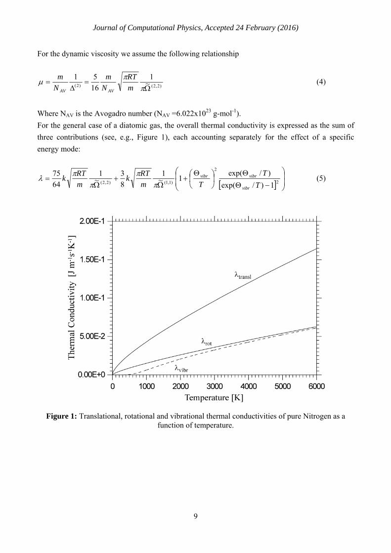
For the general case of a diatomic gas, the overall thermal conductivity is expressed as the sum of

three contributions (see, e.g., Figure 1), each accounting separately for the effect of a specific

energy mode:

2

2

)1,1()2,2( 1)/exp(

)/exp(1~

1

8

3~

1

64

75

T

T

Tm

RTk

m

RTk

vibr

vibrvibr

(5)

Figure 1: Translational, rotational and vibrational thermal conductivities of pure Nitrogen as a function of temperature.


10

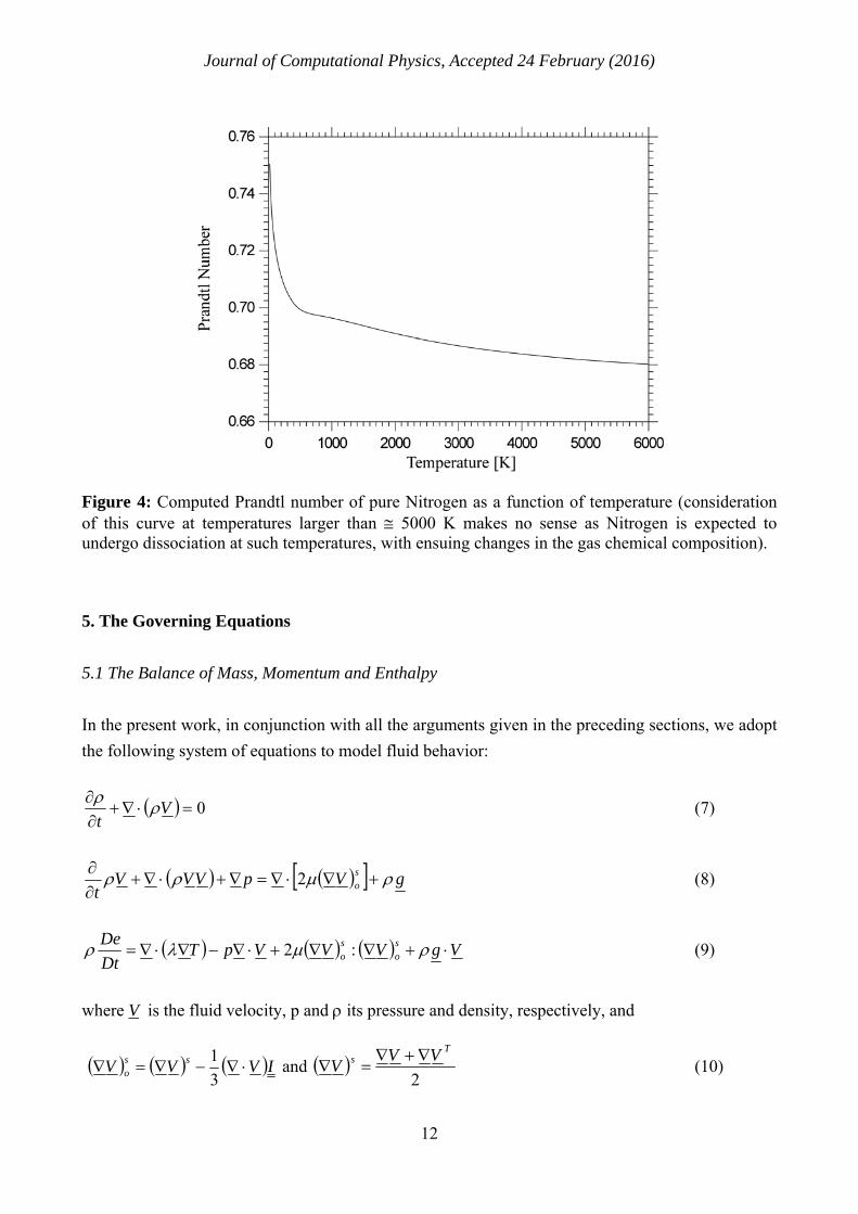
The resulting gas Prandtl number is cast in compact form as

22

)1,1()2,2(

2

22

)2,2(

)/exp(1)/exp(~1

8

3~

1)/exp(

64

75

)/exp(1)/exp(2

7~

1

16

5

)(Pr

TTT

T

TTT

Tvibr

vibrvibrvibr

vibrvibrvibr

eff

(6)

where )1,1(~ and )2,2(~ are the socalled collision cross-sections (see again the appendices).

In the following we concentrate on nitrogen as a typical paradigmatic diatomic gas.

Nitrogen is an inert, neutral and colorless gas. Apart from being one of the main components of air,

it has been one of the most important reference fluids for both tests of physical models and for the

calibration of experimental equipment. More than 14000 experimental data for many types of

thermodynamic properties are available in the fluid region of nitrogen (Yos [74]; Wood et al. [75];

Span et al. [76]; Lemmon and Jacobsen [77] and references therein). Together with water, argon,

methane, ethylene and carbon dioxide, nitrogen belongs to the group of substances possessing the

most extensively published data sets.

For temperatures between 20 and 500 K, the heat capacity can be calculated as a classical rigid-

rotor and harmonic oscillator with an uncertainty of 0.01%. Below about 15 K, the quantum effects

on the heat capacity of nitrogen isotopes become significant because the molecules of this gas have

a low rotational characteristic temperature (around 2.8 K).

At high temperatures (above 2000 K), additional contributions occur from the high vibrational

characteristic temperature (about 3400 K) as well as from a high electronic characteristic

temperature of about 72000 K for the first excited electronic state.

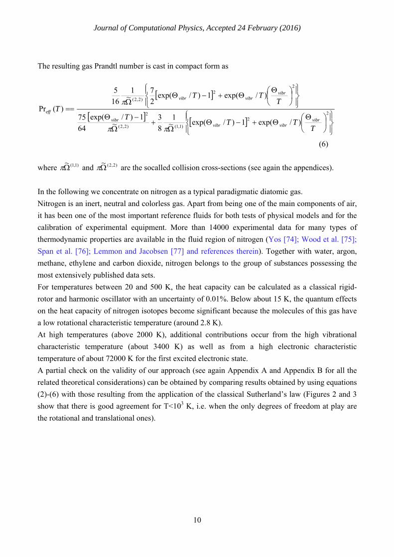
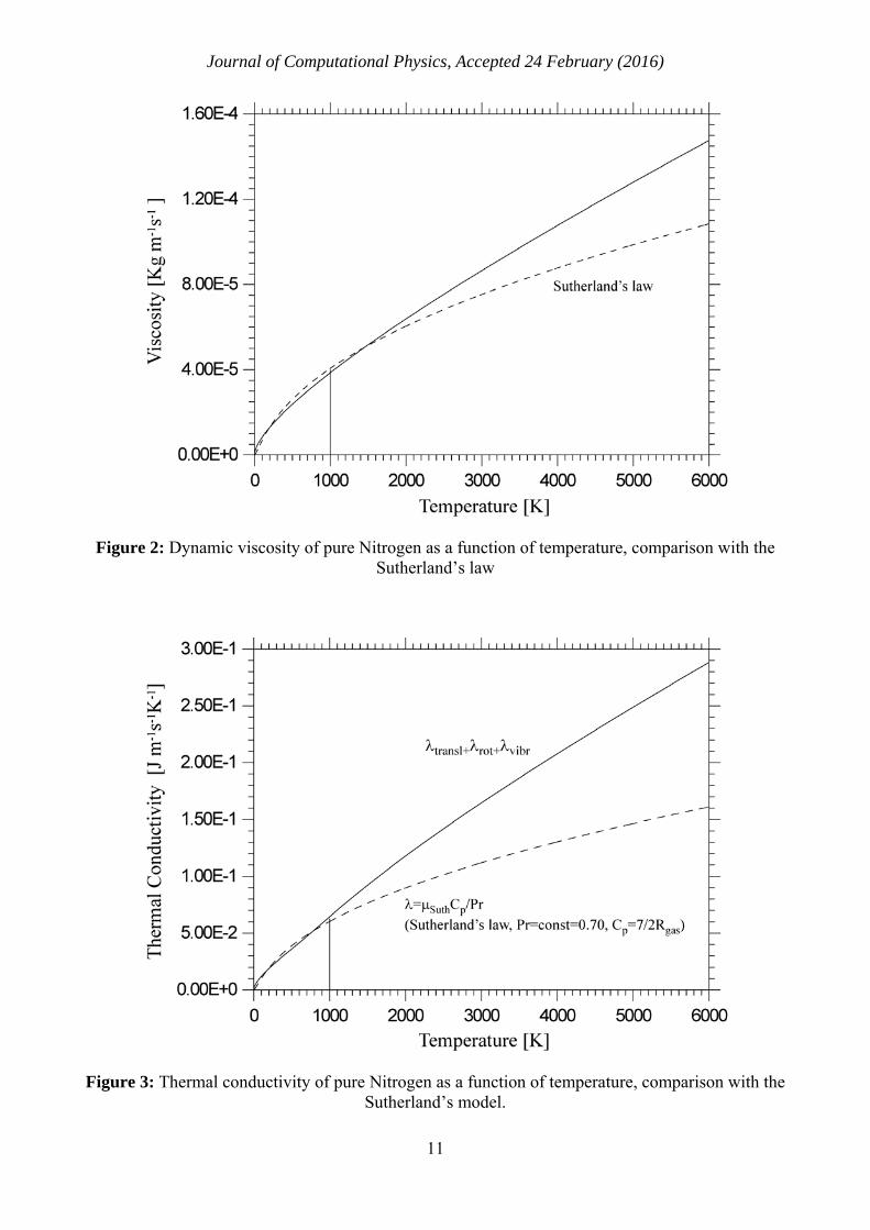
A partial check on the validity of our approach (see again Appendix A and Appendix B for all the

related theoretical considerations) can be obtained by comparing results obtained by using equations

(2)-(6) with those resulting from the application of the classical Sutherland’s law (Figures 2 and 3

show that there is good agreement for T<103 K, i.e. when the only degrees of freedom at play are

the rotational and translational ones).


11

Figure 2: Dynamic viscosity of pure Nitrogen as a function of temperature, comparison with the Sutherland’s law

Figure 3: Thermal conductivity of pure Nitrogen as a function of temperature, comparison with the Sutherland’s model.


12

Figure 4: Computed Prandtl number of pure Nitrogen as a function of temperature (consideration of this curve at temperatures larger than 5000 K makes no sense as Nitrogen is expected to undergo dissociation at such temperatures, with ensuing changes in the gas chemical composition).

5. The Governing Equations

5.1 The Balance of Mass, Momentum and Enthalpy

In the present work, in conjunction with all the arguments given in the preceding sections, we adopt

the following system of equations to model fluid behavior:

0

Vt

(7)

gVpVVVt

so

2 (8)

VgVVVpTDt

De so

so :2 (9)

where V is the fluid velocity, p and its pressure and density, respectively, and

IVVV sso

3

1

and

2

Ts VV

V

(10)


13

TRp gas (11)

As already mentioned, the Boussinesq incompressible model cannot be used if the temperature

variations are large even if the Mach number is extremely low (Gray and Giorgini [13]; Paolucci

[34]).

Here, in particular, following earlier works (Beccantini et al. [15], Bouloumou et al. [49]), we move

from an internal-energy to a specific-enthalpy formulation in order to put the equations in a form

suitable for the derivation and ensuing utilization of the socalled low-Mach approximation

repeatedly mentioned in the preceding pages. Introducing the specific enthalpy as h = e + p/,

taking into account that in terms of substantial derivatives the following expression holds

Dt

Dp

Dt

Dp

Dt

Dh

Dt

De 2

1 (12a)

which, using the continuity equation, in turn can be rewritten as:

Vp

Dt

Dp

Dt

Dh

Dt

De

1

(12b)

by substituting the above expression in the energy equation, we finally cast the balance equation for

enthalpy in condensed form as

VgVVTDt

Dp

Dt

Dh so

so :2 (13)

where TReTCTCTReeeh gasvibrVtrotVtranslgasvibrrottransl

gasvibr

vibrvibr R

Te

1)/exp(

(14)

For the convenience of the reader, it should be pointed out that the above expression defines an

implicit relation between h and T, which needs a separate treatment (in order to be in a position to

determine T as a function of h as provided by the solution of eq. 13). Towards this end (we will be

more precise later), here, we conveniently introduce a linear relationship between evibr and T by

introducing a coefficient VvibrC~

(se Figure 5) defined as:

gasvibr

vibrvibrVvibr R

T

T

T

eC

1)/exp(

/~

(15)


14

that has to be computed numerically “a priori”, i.e. before entering the effective solution process of

the system of equations (7-13). Accordingly, the specific enthalpy can be formally expressed as a

“quasi-linear” function of temperature:

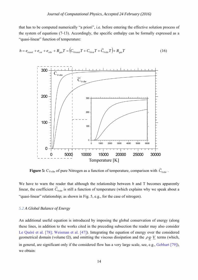
TRTCTCTCTReeeh gasVvibrVtrotVtranslgasvibrrottransl

~ (16)

Figure 5: CVvibr of pure Nitrogen as a function of temperature, comparison with VvibrC~

.

We have to warn the reader that although the relationship between h and T becomes apparently

linear, the coefficient VvibrC~

is still a function of temperature (which explains why we speak about a

“quasi-linear” relationship; as shown in Fig. 5, e.g., for the case of nitrogen).

5.2 A Global Balance of Energy

An additional useful equation is introduced by imposing the global conservation of energy (along

these lines, in addition to the works cited in the preceding subsection the reader may also consider

Le Quéré et al. [78]; Weisman et al. [47]). Integrating the equation of energy over the considered geometrical domain (volume ), and omitting the viscous dissipation and the Vg terms (which,

in general, are significant only if the considered flow has a very large scale, see, e.g., Gebhart [79]),

we obtain:


15

dsn

Ted

t

(17a)

where the second integral involves the heated or cooled boundaries of the considered geometry.

Equation (17a) accounts for the internal energy conservation over the total volume. By expressing e

as the sum of the related translational, rotational and vibrational contributions and taking into

account that Cvtransl and Cvrot can be assumed to be constant and independent of temperature, the

above expression can be expanded as

det

dsn

TTdCC

t vibrrotVtranslV (17b)

By multiplying by the gas constant Rgas and dividing each term by the constant quantity (Cvtransl +

Cvrot), the balance of energy can be also conveniently rewritten as:

detCC

Rds

n

T

CC

RRTd

t vibr

rotVtranslV

gas

rotVtranslV

gas 111 (17c)

Finally, using the equation of state to replace RT with the pressure, this equation is cast in compact

form as:

detCC

Rds

n

T

CC

R

dt

dPvibr

rotVtranslV

gas

rotVtranslV

gas 11 (18a)

where

RTdP 1 (18b)

may be regarded as a “space-averaged pressure”.

5.3 Non dimensional formulation and Characteristic Numbers

The main motivation of the present section is the selection of characteristic scales for length, time,

density, velocity, pressure, temperature and so on, so that the governing equations introduced in the

earlier sections are conveniently made dimensionless:

medgas

tref TR

P0 (19a)

medTTref (19b)


16

refrefref (19c)

medTTrottranslref

(19d)

gasVref RC (19e)

gasref

refref

R2

7

(19f)

2

2

Lp refref

ref

(19g)

LV ref

ref

(19h)

refref

Lt

2

(19i)

Where L is a reference length,

0tP is the system pressure at the initial instant t=0 (assumed to be

uniform) and ref and αref are the reference gas kinematic viscosity and thermal diffusivity,

respectively. T is the considered temperature difference.

The nondimensional temperature is introduced as T

TTT ref

* and, accordingly,

TReh gasrefref . Tref is assumed equal to the average gas temperature at the initial instant t=0

(Tref = Tmed).

The resulting grouping of physical properties and characteristic scales form dimensionless numbers

which represent ratios of various forces or quantities:

medT

T (20)

)(PrPr refeffref

ref T

(21)

2

2

ref

gas TLR

(22)

For problem closure, these 3 independent nondimensional numbers must be supplemented with the

relevant value of the Rayleigh number. Given the compressible nature of the flow (and our declared

intention to drop out the Boussinesq approximation), an adequate definition of this nondimensional

parameter is not straightforward as one may expect. Here, we define it by analogy with the

equivalent expression traditionally used in the context of studies dealing with incompressible

(Boussinesq) buoyancy convection (Lappa [11]):


17

refref

T TLgRa

3

(23)

where the socalled isobaric thermal expansion coefficient (from a formal point of view this can be

obtained by considering the density multivariate Taylor expansion in series and neglecting all the

terms of order higher than one)

constpT T

1

(24a)

generally assumed to be an intrinsic property of the fluid, is computed by resorting to the equation

of state (=p/RT) as follows:

TRT

p

T constpT

1112

(24b)

Following a common practice in the literature, in particular, we assume T=1/Tmed

refrefmedT

TLgRa

3 (25)

5.4 Low-Mach-Number Asymptotics

For many applications, the equations in Sects. 5.1 And 5.2 are too complex and broad in scope. In

the absence of observational information to properly constrain the model, a reduction of them is

beneficial. As already explained to a certain extent in Sect. 2, a commonly used approach is to

project such equations in a low-Mach-number space of parameters.

The related procedure envisages that all the primitive variables of the flow are expanded in power

series law of a small parameter M2 << 1 (where, obviously, M is the reference Mach number).

222*

1*0

* )(MOM (26a)

222*1

*0 )(MOMppp (26b)

222*1

*0 )(MOMVVV (26c)

222*1

*0 )(MOMTTT (26d)


18

To derive the low Mach number equations, primitive variables are substituted by their expansions in

the fully compressible Navier-Stokes equations in non-dimensional form and the lowest order terms

in M2 are collected (Beccantini et al. [15]; Benteboula and Lauriat [48]).

At the order -1, the non-dimensional momentum equation reduces to:

0*

0 p (27)

At the order zero, the following low-Mach number governing equations are obtained for mass and

momentum:

*

*0*

0*0 tV

(28)

*0

*0

*0

*1

*0

*0

*0

*0

*0*

Pr2Pr

Ra

VpVVVt

s

o

(29)

with the state equation:

1*

0*0

*0

Tp (30)

being required to recover the density *

0 (r, t).

It becomes evident at this stage that the most important outcome of the low Mach number

approximation is the possibility to split the pressure into two components; a thermodynamic

pressure p0 homogeneous in space and allowed to vary in time, and a dynamic pressure p1

decoupled from density and temperature fluctuations.

The reader will also easily realize that the homogeneous pressure p0 will be playing essentially the

role of the average pressure defined by eq. (18b) (Beccantini et al. [15] Benteboula and Lauriat [48],

Le Quéré et al. [78]); the second pressure p1 is decoupled from the density, so that the

decomposition eliminates acoustic waves.

Let us recall that, as already outlined in Sect. 2, density variations are responsible for fast acoustic

waves which are the major source of issues in time-advancing numerical algorithms (indeed, due to

their speed of propagation that is two or three orders of magnitude larger than the convective

velocities, very small time integration steps must be used to guarantee algorithm stability).

Moreover, such waves play generally no significant role in typical problems of thermal convection.

In the following for the sake of clarity, the subscripts related to the asymptotic expansions will be

omitted, with the zero-th and first order pressure contributions p0 and p1 simply indicated as P and

p’, respectively.


19

Denoting for simplicity by class the ordinary thermal conductivity (accounting for the influence of translational and rotational degrees of freedom only), i.e. rottranslclass , the global energy

balance (evolution in time of the thermodynamic pressure) simply reads:

**

*

***

**

*

5

2

5

7dS

n

T

dt

dPvibrclass where ***

*

det vibr (31)

where it is easy to recognize (via the equation of state) that the first term simply accounts for the

change in time of the (constant in space) thermodynamic pressure.

For the specific enthalpy balance we have:

*

******

*

**

7

2

dt

dPThV

t

hvibrclass

(32)

where *1*1***** 112

3vibrvibrrottransl eTTeeeh

and

1***

02**

**2

*

** ~

1)/exp(

)/exp(*

TCdTT

T

Te Vvibr

T

vibr

vibrvibrvibr

1**1***** 1~

12

3

TCTeeeh Vvibrvibrrottransl

*

1**

*

~

2

7

~

2

7

Vvibr

Vvibr

C

Ch

T

(33)

To summarize, in the above equations the conservation of internal energy has been obtained

neglecting the contribution of the dynamic pressure in the internal energy and the viscous

dissipation, while in the time-evolution equation for the enthalpy, we have discarded the term O(M2)

in the pressure asymptotic expansion as well as the temperature variation due to the viscous

dissipation. In all the equations, the density has been replaced using the (asymptotic) equation of

state, in which the contribution of the dynamic pressure is neglected.

It is also worth highlighting that, as already explained to a certain extent in Sect. 5.1, *~VvibrC

appearing in the above relationship does depend on T*, which implies that eq. (33) has to be solved

resorting to an iterative process.


20

6. The modified projection method for high-temperature gases

Hereafter, for brevity asterisks used to denote nondimensional quantities are omitted.

Let us start from the simple remark that a property common to all variants of the projection method

is their ability to proceed as a type of fractional step method by first writing a modified momentum

equation and then updating the velocity field using the computed pressure to account for the

continuity equation. More precisely, at each time step, an intermediate field V~~ is determined

without the knowledge of the correct pressure field, and therefore no condition related to the

conservation of mass is enforced. The intermediate velocity field is then corrected by a second step

in which a pressure equation is solved and then the computed pressure is used to produce a velocity

field satisfying the continuity equation.

In the first step, the approximate (often also referred to as the “provisional”) field V~~ can be

computed neglecting the gradient of dynamic pressure in the momentum equation, i.e.,

n

so

nn RaVVVtVV

Pr

2Pr~~ (34)

In the second substep, the dynamic pressure field must be computed by solving a Poisson equation

introduced using the continuity equation tV nn /11 and taking into account that 11 nn V is related to V

~~ by the relationship ptVV nn ~~11 :

t

ptVV nn

~~11

t

Vpt

~~2 (35)

Finally, the velocity field can be updated using the computed dynamic pressure field to account for

continuity:

ptVVnn

n

11

1 1~~1

(36)

6.1 Spatial discretization

In our simulations we cover the computational domain with a staggered grid, the fluxes and

velocities being located at the centers of the faces and, the scalar variables density, temperature and

pressure at the center of the cells. A centered finite-difference scheme with a second-order accuracy

is retained for the spatial discretization. However, we use a third-order-accurate upwind scheme for


21

the convective terms in the energy equation. To this end, the convective term V has to be

reformulated as

VVV (37)

The third-order-accurate upwind scheme is applied only to the conservative part V .

This scheme appears to be necessary for high density ratios in order to damp the spurious

oscillations introduced by the centered treatment of convective terms (see Benteboula and Lauriat

[48]).

6.2 Time discretization

A second-order backward scheme is then employed for approximating the time derivative at the

right-hand side of the elliptic (Poisson) equation. It reads

tt

nnn

2

43 11 (38)

This term is generally an instability source for such an algorithm, as reported in Nicoud [44], Cook

and Riley [43] and Benteboula and Lauriat [48].

6.3 Outline of the time marching procedure

Our effective resolution process is finally articulated into four main macro stages of computation.

First macro stage:

The time derivative of the integral related to the vibrational energy at the right-hand side of eq. (31),

denoted by , is discretized with a first-order backward scheme involving known quantities at tn

and tn-1:

dTCdTC

tde

tnn

Vvibrnnn

Vvibrn

n

vibrn 11111 ~~1 (39)

Second macro stage:

A second-order explicit Adams-Bashforth scheme is used to advance in time thermodynamic

pressure and enthalpy:


22

nn

nvibr

nclass

nnvibr

nclass

nn tdSn

TtdS

n

TtPP

5

2

5

7

2

1

5

7

2

3 1111

(40)

11

1111

11

11

1

7

2

2

11

2

1

1

7

2

2

31

2

3

nnn

nnvibr

nclassn

nn

nnn

nnvibr

nclassn

nnnn

PPThVt

PPThVthh

(41)

Temperature is determined accordingly (via an iterative process) through its relationship with the

specific enthalpy:

kVvibr

kVvibr

n

k

C

Ch

T~

2

7

~

2

7 11

1

assuming )(

~~ nVvibr

kVvibr TCC for k=1 and )(

~~ kVvibr

kVvibr TCC for k>1

(42)

(in general, two or three iterations are sufficient to attain convergence).

Density is computed via the state equation using the newly determined values of P and T:

11

11

n

nn

T

P (43)

Third macro stage:

The intermediate (provisional) momentum field is computed as:

111111 Pr2Pr

2

1

Pr2Pr

2

3~~

ns

onnnnn

ns

onnnnnnn

RaVVVt

RaVVVtVV

(44)

And the dynamic pressure is computed solving the equation:

t

Vptnnn

2

43~~11

2 (45)


23

Final stage

ptVVnn

n

11

1 1~~1

(46)

n+1=(Tn+1), n+1=(Tn+1) , )(~~ 11 n

Vvibrn

Vvibr TCC (47)

7. The benchmark problem and its extensions

As indicated at the end of Sect. 3, our overall framework has been built via the integration of self-

contained modules, which could be individually tested.

However, because it is crucial that the entire numerical architecture is tested as a single integrated

unit, we considered available solutions in the literature for comparison.

To enhance progress in this field of study, several benchmark problems have been defined for

natural (buoyancy) convection in closed cavities and enclosures. These benchmarks have been

specifically conceived to allow the validation of newly developed numerical approaches and

algorithms.

Though most of these studies were concentrated on cases with low temperature gradients where the

Boussinesq assumption is definitely valid (for example, one of these is the benchmark solution

discussed by DeVahl Davis [79,80], see also Bucchignani [81]), however, in 2000 the CEA Nuclear

Reactor Division of the French Atomic Energy Commission organized a workshop at the Institut

National des Sciences & Techniques Nucléaires (INSTN) in Saclay, France (CEA [82]) to account

for the effect of compressibility. In the call for contributions to this workshop, a new benchmark

problem was designed around the extension of the incompressible de Vahl Davis benchmark

problem to cases with large temperature differences imposed upon the vertical walls (see, e.g.,

Paillère and Le Quéré [83]). Eight test cases, simulating air at a prescribed Rayleigh number of Ra

= 106 in a two-dimensional square cavity (see Fig. 6) were defined by fixing four non-dimensional

temperature differences and both constant and variable viscous and thermal diffusion coefficients,

with the temperature dependent coefficients modelled by the Sutherland’s Law. Four years later, the

results presented at such a workshop were further refined in the framework of the conference on the

Mathematical and Numerical Aspects of Low Mach Number Flows organized by INRIA and MAB

[84] in Proquerolles, France. The results by different participants were collected in a couple of

papers (Le Quéré et al. [78]; Paillère et al. [85]).


24

Figure 6: Square cavity with adiabatic bottom and top walls and lateral walls at different temperatures (no slip conditions along the entire boundary).

As a sensitive parameters for comparison, participants decided to concentrate on the value of the

Nusselt number (Nu). For the sake of consistency with the definition of Nu used by such author,

here we define it as:

dyyNuL

Nu loc

L

)(1

0 where

wallvibrrottransl

oloc x

T

T

LyNu

)()(

)(

, medTTrottranslo

(48)

(such a definition guarantees that in the absence of vibrational effects, our definition of the Nusselt

number matches exactly the one considered by these authors).

Table I illustrates the comparison between the results presented at the two aforementioned

congresses and those obtained using the present numerical code.


25

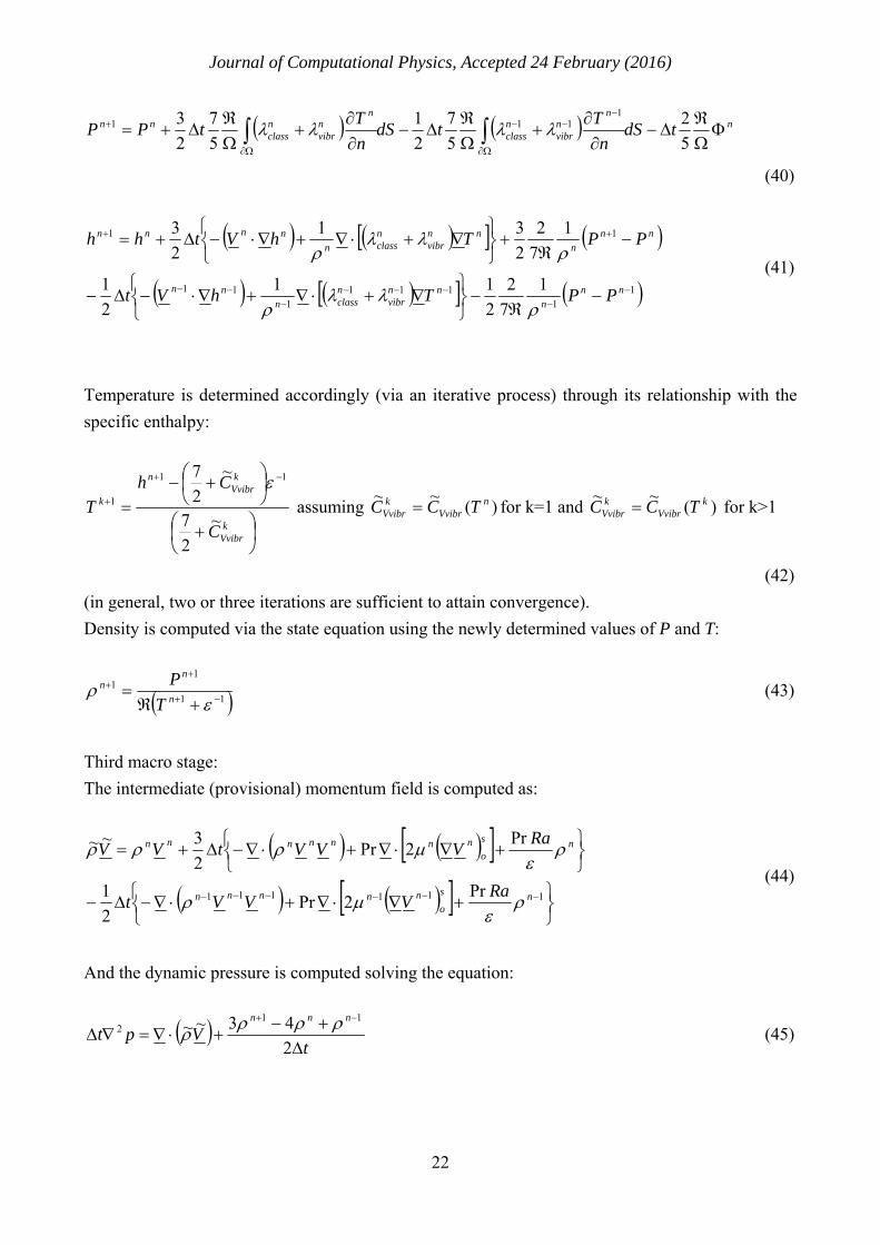
Table I: Comparison between the present numerical results and earlier results by other authors (data considered for the simulations: air, Po = 101325 [Pa], Tmed=To=600 [K], Rgas = 287 [J kg-1K-1], ρo = Po/RgasTo, γ = 1.4, g = 9.81 [ms-2], Pr = 0.71, Ra=106).

Tcold [K] Thot [K] Nucold Nuhot Viscosity Author

594 606 8.8 8.8 Constant de Vahl Davis

594 606 8.8133 8.8112 Constant Present

240 960 8.6866 8.6866 Sutherland’s CEA 2000

240 960 8.6866 8.6866 Sutherland’s Vierendeels

240 960 8.6866 8.6866 Sutherland’s Braack

240 960 8.6855 8.6916 Sutherland’s Dabbene

240 960 8.6747 8.6868 Sutherland’s Beccantini

240 960 8.6338 8.6953 Sutherland’s Kloczko

240 960 8.6861 8.6889 Sutherland’s Heuveline

240 960 8.7150 8.7150 Sutherland’s Darbandi

240 960 8.7135 8.7160 Coll. Int. Present

The reader will easily realize that the present results agree with those by other authors within a

percentage less that 2%. Perhaps, the small difference noticeable for the case with larger

temperature difference (Thot=960 K, Tcold=240 K,) with respect to the other results might be justified

by taking into account that we did not use the Sutherland’s law to reproduce the results of the

benchmark. Rather, towards the end of further testing the code subroutines and their reliability, we

carried out the simulation using for viscosity and thermal conductivity the more general laws shown

in Figs 2 and 3, respectively. Although we derived such curves for the case of pure diatomic

Nitrogen, they may be regarded as a good approximation of the Sutherland’s law for air as well for

T<103 K (see, e.g., Gupta et al. [86]).

At this stage, it should be clearly pointed out that the range of temperature considered for the

benchmark (240 < T < 960 K) is not sufficient to excite the vibrational degree of freedom of the air

components (let us recall that, as reported in the Appendix B, the characteristic vibrational

temperatures vibr of Oxygen and Nitrogen, as obtained from spectroscopic data, are 2270 K and

3390 K, respectively), which means the only NOB effects at play in such simulations were the gas

compressibility and the dependence of viscosity and thermal conductivity on temperature (via the

Sutherland’s law).

In order to extend the benchmark to a case where the vibrational degree of freedom does a play a

role and the departures from the Sutherland’s law become significant for viscosity, thermal

conductivity and specific heat coefficient, we have considered Nitrogen at an average temperature

of 3500 K (as shown in Fig. 4, the related value of the Prandtl number, Pr0.69, is relatively close

to the one that was considered for the 2004 benchmark, Pr=0.71). In particular, we have assumed as


26

thermal conditions on the lateral cold and hot walls, a temperature well below and well above the

characteristic vibrational temperature of Nitrogen (Tcold=2000 K< vibr< Thot=5000 K).

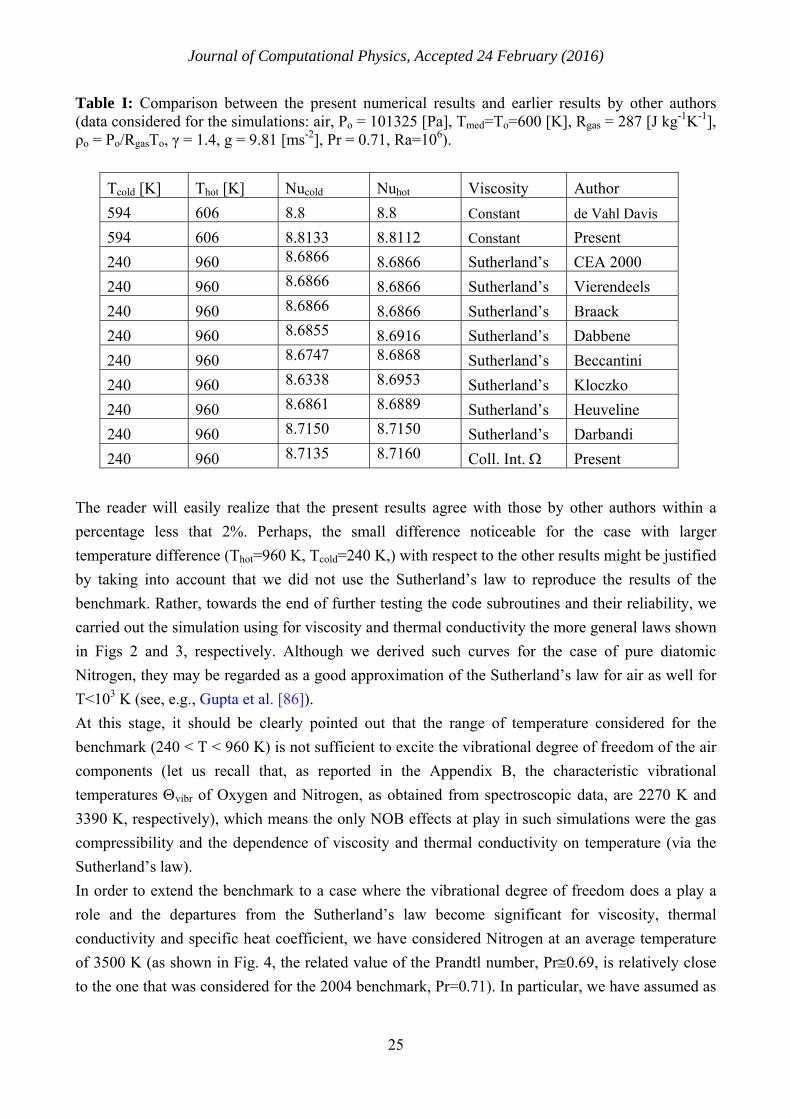
The results shown in Fig. 7, reveal that while the thermofluid-dynamic field does not show

significant qualitative changes with respect to the pattern obtained for the benchmark test case (see,

e.g., Darbandi and Hosseinizadeh [60]), the Nusselt number is shifted to a slightly lower value

Nu8.512159.

Figure 7: Thermofluid-dynamic field (steady state) in a square cavity filled with Nitrogen gas (lateral walls at temperatures Tcold=2000 K and Thot=5000 K, respectively, Nu=8.512159, adiabatic bottom and top walls, grid 320x320, max/min2.6).

According to the present results, however, the most interesting changes (induced by the excitation

of the vibrational degree of freedom in the flow and related NOB effects) emerge when the

direction of the temperature gradient is rotated by 90 with respect to the direction considered in the

benchmark, i.e. when the temperature gradient and the gravity acceleration have the same direction.

This leads us to the well-known Rayleigh-Bénard (RB) convection problem that so much attention

has attracted in the literature due to its relevance to a number of natural and industrial processes

[11,12]. This kind of convection presents, during the evolution from the stationary state to the fully

developed turbulent regime, such a rich scenario of different structures and bifurcations that it is

widely regarded as a reference problem for the study of different transition mechanisms in fluid

dynamics ([87-93]).

When the Rayleigh number is increased beyond a certain critical threshold, it is known that even

under the nonphysical constraint of two-dimensional flow in a square cavity, RB convection can

undergo transition to relatively complex and/or time-dependent regimes. A rigorous categorization

of solutions in terms of the related symmetries can be found in Mizushima [94]. In general, the

distinct modes of convection can be delineated by considering various combinations of the possible

symmetries along the horizontal and vertical directions. This leads to partition the set of possible

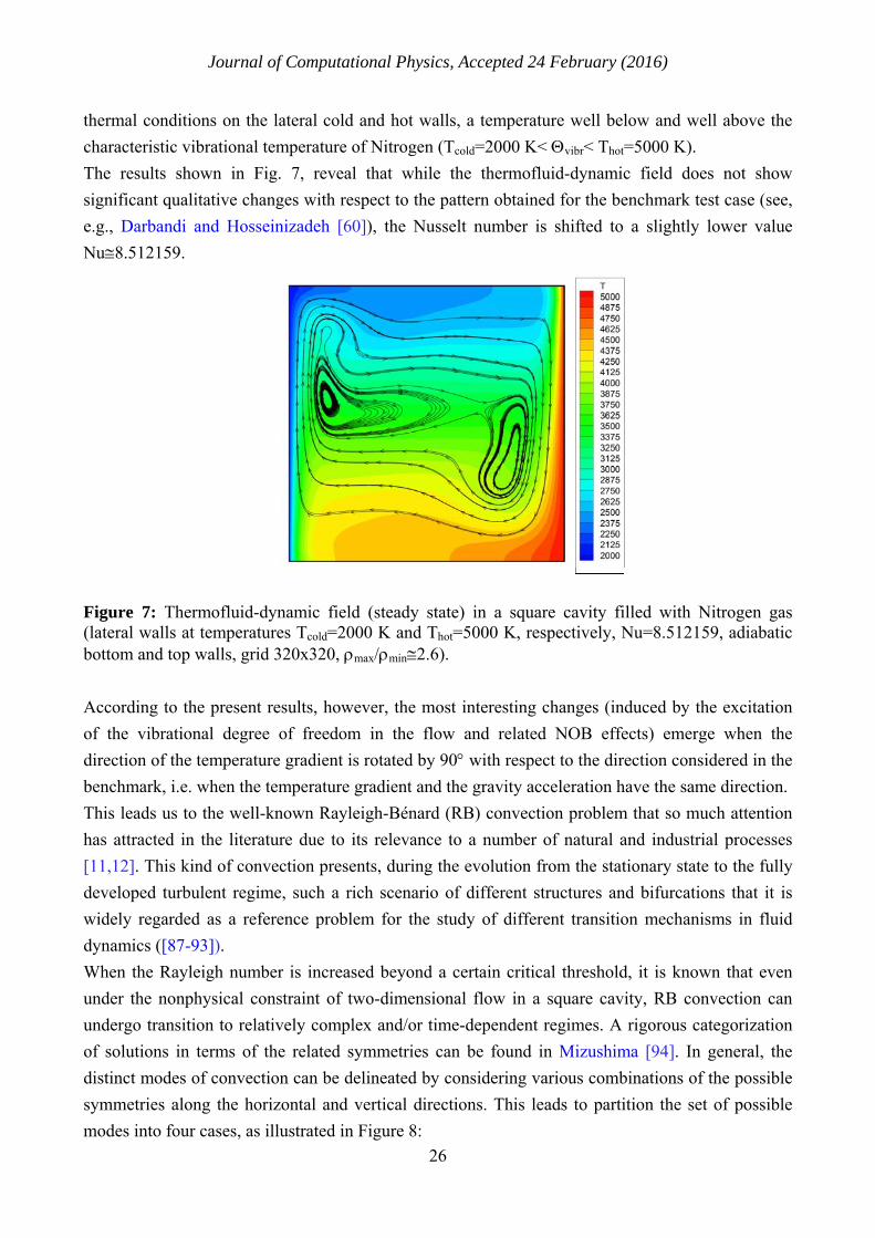
modes into four cases, as illustrated in Figure 8:


27

Fig. 8: Categorization of possible solutions of RB convection in 2D finite enclosures in terms of related symmetries.

• (aa): The antisymmetric–antisymmetric mode. This mode has an odd number of vortex cells along

both the horizontal and the vertical directions.

• (sa): The symmetric–antisymmetric mode. This mode is characterized by an even number of rolls

along the horizontal direction and an odd number of vortices along the y direction.

• (as): The antisymmetric–symmetric mode. This mode exhibits an odd number of rolls along x and

an even number of cells in the perpendicular direction.

• (ss): The symmetric–symmetric mode. This mode has an even number of vortex cells along both

the horizontal and the vertical directions.

In practice, due to the symmetry/antisymmetry properties of the governing equations and of the

boundary conditions, different solutions can appear which can be obtained by reflection about the

vertical cavity centreline (parallel to the applied temperature gradient), about the horizontal cavity

centerline (perpendicular to the gradient) and about both of them.

In particular, as originally illustrated by Mizushima and Adachi [95], for Pr=O(10) it is known that

the initial modes with the (aa) or (sa) symmetries can produce modes with different symmetries via

a nonlinear interaction mechanism when the Rayleigh number is sufficiently high.

In the following, in particular, we concentrate on Ra=106, such a choice (although it was used for

the benchmark as well) being motivated by the earlier numerical results by Goldhirsch et al. [96],

who found (for this specific value of the Rayleigh number, for Pr=0.71 and for incompressible flow

and constant thermodynamic properties) the solution to be characterized by the unusual (as)

symmetry. For this value of the Prandtl number, they also identified this specific value of the

Rayleigh number as a threshold value roughly separating steady solutions (for smaller values of Ra)

from oscillatory solutions (for larger values of Ra).

Although we consider pure Nitrogen, Figure 9, shows that when the behaviour can be considered

incompressible (very small value of the temperature gradient, 1 K only) and the average

temperature is much smaller than the vibrational characteristic temperature, the emerging solution is

very similar to that obtained by Goldhirsch et al. [96].


28

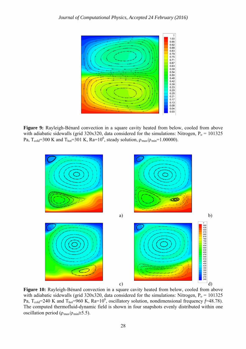
Figure 9: Rayleigh-Bénard convection in a square cavity heated from below, cooled from above with adiabatic sidewalls (grid 320x320, data considered for the simulations: Nitrogen, Po = 101325 Pa, Tcold=300 K and Thot=301 K, Ra=106, steady solution, max/min=1.00000).

a) b)

c) d) Figure 10: Rayleigh-Bénard convection in a square cavity heated from below, cooled from above with adiabatic sidewalls (grid 320x320, data considered for the simulations: Nitrogen, Po = 101325 Pa, Tcold=240 K and Thot=960 K, Ra=106, oscillatory solution, nondimensional frequency f=48.78). The computed thermofluid-dynamic field is shown in four snapshots evenly distributed within one oscillation period (max/min5.5).


29

Figure 11: Computed Nusselt number for the same configuration shown in Fig. 10 (Nuhot-solid line,

Nucold-dashed line).

Figure 12: Rayleigh-Bénard convection in a square cavity heated from below, cooled from above with adiabatic sidewalls (grid 320x320, data considered for the simulations: Nitrogen, Po = 101325 Pa, Tcold=2000 K< vibr< Thot=5000 K, Ra=106, steady solution, max/min2.6).

Indeed, the temperature contour plot and the associated velocity field show a stationary roll-over-

roll structure with three boundary layers: two at the top and bottom plates and one in between the

rolls.

Figures 10-12, however, reveal that when NOB effects are taken into account, the symmetries of the

emerging flow change dramatically depending on the effective temperature gradient applied and the

fluid average temperature (this clearly indicates that NOB effects of various natures can exert a


30

strong influence on the pattern-symmetry selection process that takes place via the aforementioned

mode nonlinear interaction mechanism). Such effects can even change the nature of the resulting

flow from steady to oscillatory, as shown in Figs. 10 and 11.

By comparing Figs. 9 and 10, the reader will immediately realize that when the effects of

compressibility are taken into account, the perfect mirror symmetry with respect to the midsection,

seen in Fig. 9 for the case of an almost incompressible flow, should no longer be considered as a

characteristic property of the pattern. The upper roll takes a size much larger than that of the roll

affecting the lower half of the enclosure. The latter, in turn, undergoes evident oscillatory motion,

which seems to be produced by the periodic growth and decay of a secondary roll embedded in the

lower circulation system (such interpretation being consistent with the clearly observable presence

of a wave travelling along the bottom thermal boundary layer).

For Tcold=2000 K< vibr< Thot=5000 K where the effects produced by the activation of the

vibrational degree of freedom can be considered dominant, although we are still considering the

same value of the Rayleigh number (Ra=106) the flow pattern is again steady (Fig. 12). It comprises

a main convective cell with deformed shape and two smaller satellite vortices located in upper left

and in the lower right corners, respectively.

These results indicate that the mechanism originally identified by Mizushima and Adachi [95] for a

larger value of the Prandtl number is still relevant to the present case. For Pr=O(1), however, it is

driven essentially by modes with the (as) and (sa) symmetries. Being involved with different

relative amplitudes (the ratio of such amplitudes being linked to the degree of vertical asymmetry

introduced in the problem by the temperature-dependent fluid physical properties, i.e. NOB effects),

the superposition/competition of these modes gives rise to oscillatory or steady patterns. The

changes experienced accordingly by the Nusselt number are summarized in Table II.

Table II: Rayleigh-Bénard convection in a square cavity heated from below, cooled from above with adiabatic sidewalls (grid 320x320, data considered for the simulations: Nitrogen, Po = 101325 [Pa], Ra=106).

Tcold [K] Thot [K] Nucold Nuhot Solution 300 301 4.3978 4.3977 Steady

240 960 4.11

(average) 4.11 (average)

Weakly Oscillatory

2000 5000 6. 0701 6.0722 Steady

The above results should be regarded as a paradigmatic example of the significant changes that the

resulting thermofluid-dynamic field can exhibit for a fixed value of the Rayleigh number due to

NOB effects.


31

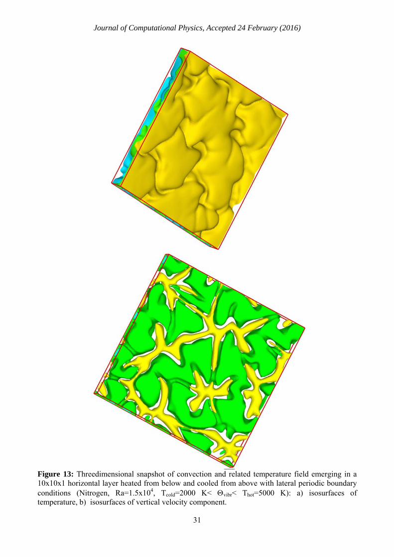
Figure 13: Threedimensional snapshot of convection and related temperature field emerging in a 10x10x1 horizontal layer heated from below and cooled from above with lateral periodic boundary conditions (Nitrogen, Ra=1.5x104, Tcold=2000 K< vibr< Thot=5000 K): a) isosurfaces of temperature, b) isosurfaces of vertical velocity component.


32

Given the intimate three-dimensional nature of this kind of flow when relatively supercritical

conditions are considered, the additional example shown in Fig. 13 has been obtained using the

fully 3D version of the present numerical code. In particular, we have considered a shallow layer

with periodic boundary conditions at the sides, for which on the basis of classical theory (the

socalled Busse balloon, see, e.g., Lappa [11]) the emerging secondary modes of RB convection for

Ra=O(104) should appear in the form of elongated oscillatory rolls.

Figure 13 clearly shows that NOB effects can cause a significant departure from the secondary

modes of RB convection in liquid layers as predicted by the classical theory. Indeed, when the

upper and lower solid surfaces bounding the layer are kept at Tcold=2000 K and Thot=5000 K,

respectively, a kind of oscillatory spoke convection appears in place of oscillating elongated rolls.

Due to page limits and not to increase further the length of this article (that has been devoted

essentially to the presentation of the numerical method and its new aspects with respects to earlier

efforts available in the literature), the detailed analysis of NOB effects expressly produced by the

activation of the vibrational degree of freedom is delayed to future studies. Other possible routes to

further expand the potentialities of the present algorithm are outlined in the conclusions.

7. Conclusions and Future directions

In this work, we addressed the question of how a departure from the known behaviour of gases at

ordinary temperatures can affect the flow and how a typical numerical framework for low-Mach-

number compressible flows can be adequately extended so to make it suitable for the simulation of

thermal (natural) flows at large temperatures and/or driving temperature gradients.

In particular, starting from existing strategies for the solution of compressible (low-Mach) thermal

convection, some effort has been provided to strengthen the used approach by incorporating in the

algorithm the possibility to account for the activation of the molecule vibrational degree of freedom.

This has required the application of a set of complementary points of view on the problem,

spanning different length scales, covering different disciplines, ranging from the classical kinetic

theory of gases, to some results provided by quantum mechanics, passing through the known

solutions of the Boltzmann equation and related Eucken extensions, taking advantage of useful

indications provided by existing asymptotic analyses and the resulting multiple-pressure-variables

approach, up to extending the class of projection methods to the case of compressible flows.

The advantage of the resulting framework lies in its capability to deal with a broad range of cases in

terms of average value of the system temperature and applied temperature difference, including

nearly incompressible flows, with a single modeling, without any need to change the

thermodynamic properties representation or to reformulate the governing equations, thereby

alleviating the user from the burden to assess for each case the best set of properties and equations

to be used.


33

We hope this will maximize the strength of this category of (projection-like) methods in enabling

new challenging problems to be addressed across the engineering and physical sciences.

As a concluding remark, we may further emphasize the advantage provided by such a framework by

pointing out how it could be easily extended to the case of non-reacting gas mixtures. Future work

shall be also devoted to considering natural convection in gases which undergo dissociation.

9. References [1] Sun Z. and Jaluria Y., (2011), Conjugate Thermal Transport in Gas Flow in Long Rectangular Microchannel, J. Electron. Packag., 133(2), 021008 (11 pages). [2] Baltasar J., Carvalho M.G., Coelho P., Costa m, (1997), Flue gas recirculation in a gas-fired laboratory furnace: Measurements and modelling, Fuel, 76(10): 919–929. [3] Lappa M. and Savino R., (2002), 3D analysis of crystal/melt interface shape and Marangoni flow instability in solidifying liquid bridges, Journal of Computational Physics, 180 (2): 751-774. [4] Lappa M., (2005), Thermal convection and related instabilities in models of crystal growth from the melt on earth and in microgravity: Past history and current status, Cryst. Res. Technol., 40(6): 531-549 [5] von Backström T. W. and Gannon A.J., (2000), Compressible Flow Through Solar Power Plant Chimneys, J. Sol. Energy Eng., 122(3): 138-145. [6] Elmo M, and Cioni O., (2003), Low Mach number model for compressible flows and application to HTR, Nuclear Engineering and Design, 222: 117–124. [7] Hu S., Henager Jr. C. H., Heinisch H. L., Stan M., Baskes M. I., Valone S. M., (2009), Phase-field modeling of gas bubbles and thermal conductivity evolution in nuclear fuels, Journal of Nuclear Materials, 392(2): 292–300 [8] Martineau R. C., Berry R. A., Esteve A., Hamman K. D., Knoll D. A., Park R., Taitano W., (2010), Comparison of natural convection flows under VHTR type conditions modeled by both the conservation and incompressible forms of the Navier–Stokes equations, Nuclear Engineering and Design, 240: 1371–1385 [9] McGrattan K.B., Baum H.R, and Rehm R.G., (1998), Large eddy simulations of smoke movement, Fire Safety Journal, 30: 161-178. [10] Valentine G.A. and Wohletz K.H., (1989), Numerical Models of Plinian Eruption Columns and Pyroclastic Flows, Journal of Geophysical Research, 94(B2): 1867-1887 [11] Lappa M., (2009). Thermal Convection: Patterns, Evolution and Stability (John Wiley & Sons, Chichester, England, 2009). [12] Lappa M., (2012), Rotating Thermal Flows in Natural and Industrial Processes (John Wiley & Sons, Chichester, England, 2012). [13] Gray D. and Giorgini A., (1976), The validity of the Boussinesq approximation for liquids and gases, Heat and Mass Transfer, 15: 545-551. [14] Munz C.-D., Roller S., Klein R., Geratz K.J., (2003), The extension of incompressible flow solvers to the weakly compressible regime, Computers & Fluids, 32(2): 173–196. [15] Beccantini A., Studer E., Gounand S., Magnaud J.-P., Kloczko T., Corre C. and Kudriakov S., (2008), Numerical simulations of transient injection flow at low Mach number regime, Int. J. Numer. Meth. Engng, 76: 662-696.


34

[16] Turkel E., (1987), Preconditioning methods for solving the incompressible and low speed compressible equations, J. Comput. Phys., 72: 277–298. [17] Volpe G., (1993), Performance of Compressible Flow Codes at Low Mach Numbers, AIAA Journal, 31(1): 49–56. [18] Guillard H. and Viozat C., (1999), On the behaviour of upwind schemes in the low Mach number limit, Comput. Fluids, 28: 63–86. [19] Mary I., Sagaut P., Deville,M., (2000), Algorithm for Low-Mach Number Unsteady Flows, Comput. Fluids, 29(2): 119–147. [20] Paillere H., Viozat C., Kumbaro A., Toumi I., (2000), Comparison of low Mach number models for natural convection, Heat and Mass Transfer, 36(6): 567–573. [21] Vierendeels J., Merci B., and Dick E., (2001), Numerical Study of Natural Convective Heat Transfer with Large Temperature Differences, International Journal of Numerical Methods for Heat and Fluid Flow, 11(4): 329–341. [22] Parchevsky K.V., (2001), Numerical simulation of sedimentation in the presence of 2D compressible convection and reconstruction of the particle-radius distribution function, Journal of Engineering Mathematics, 41: 203-219. [23] Könözsy L. and Drikakis D., (2014), A Unified Fractional-Step, Artificial Compressibility and Pressure-Projection Formulation for Solving the Incompressible Navier-Stokes Equations, Communications in Computational Physics, 16(05): 1135-1180 [24] Kothe D.B., Ferrell R.C., Turner J.A., Mosso S.J., (1997), A high resolution finite volume method for efficient parallel simulation of casting processes on unstructured meshes, presented at the 8th SIAM Conference on Parallel Processing for Scientific Computing, Minneapolis, MN, March 14–17, 1997 [25] Moukalled F. and Darwish M., (2001), A High-Resolution Pressure-Based Algorithm for Fluid Flow at All Speeds, Journal of Computational Physics, 168(1): 101–133. [26] Harlow F.H. and Welch J.E., (1965), Numerical calculation of time-dependent viscous incompressible flow with free surface, Phys. Fluids, 8: 2182-2189. [27] Harlow F., Shannon J. and Welch J., (1965), THE MAC METHOD: A Computing Technique for Solving Viscous, Incompressible, Transient Fluid-Flow Problems involving Free Surfaces, Technical Report LA-3425, Los Alamos Scientific Laboratory (1965). [28] Chorin A.J., (1968), Numerical solutions of the Navier-Stokes equations, Math. Comput., 22: 745-762. [29] Temam R., (1968), Une méthode d'approximation de la solution des équations de Navier-Stokes, Bull. Soc. Math. France, 98: 115-152. [30] Temam R., (1969), Sur l'approximation de la solution des èquations de Navier-Stokes par la mèthode des pas fractionnaires (I), Arch. Rat. Mech. Anal., 33: 377-385. [31] Ladyzhenskaya O.A., (1969), The Mathematical Theory of Viscous Incompressible Flow, Gordon and Breach, 2nd Edition, New York - London, 1969. [32] Gauthier S., (1988), A spectral collocation method for two dimensional compressible convection, J Comput. Phys., 75(1): 217–35. [33] Casulli V. and Greenspan D., (1984), Pressure method for the numerical solution of transient, compressible fluid flows, Int. J. Numerical Methods in Fluids, 4: 1001-1012. [34] Paolucci S., (1982), On the filtering of sound from the Navier–Stokes equations, Technical Report SAND 82-8251, Sandia National Laboratories, Livermore, 1982.


35

[35] Majda A., and Sethian J., (1985), The derivation and numerical solution of the equation for zero Mach number combustion, Combust. Sci. Technol., 42(3-4): 185-205. [36] Klein R., (1995), Semi-implicit extension of a godunov-type scheme on low Mach number asymptotics, J. Comput. Phys., 121: 213-237. [37] Meister A., (1999), Asymptotic single and multiple scale expansions in the low Mach number limit, SIAM Journal on Applied Mathematics, 60: 256–271. [38] Roller, S. and Munz, C.-D., (2000), A low Mach number scheme based on multi-scale asymptotics, Comput. Visual. Sci., 3 (1/2 500): 85–91. [39] Müller B., (1998), Low Mach number asymptotics of the Navier–Stokes equations, J. Eng. Math. 34(1-2), 97–109. [40] Chenoweth D. R. and Paolucci S., (1986), Natural Convection in an Enclosed Vertical Air Layer with Large Horizontal Temperature Differences, J. Fluid Mech., 169: 173–210. [41] Fröhlich J. and Gauthier S., (1993), Numerical investigations from compressible to isobaric Rayleigh–Bénard convection, Eur. J. Mech. B, 12: 141–59. [42] Crockera D. S. and Paranga M., (1994), Thermally driven convection in enclosed compressible fluids, Numerical Heat Transfer, Part A, 26(5): 569-585. [43] Cook A.W. and Riley J.J., (1996), Direct numerical simulation of a turbulent reactive plume on a parallel computer, J. Comput. Phys. 129(2): 263–283. [44] Nicoud F., (2000), Conservative high-order finite-difference scheme for low-Mach number flows, J. Comput. Phys., 158(1): 71–97. [45] Hung K. S. and Cheng C. H., (2002), Pressure Effects on Natural Convection for Non-Boussinesq Fluid in a Rectangular Enclosure, Numer. Heat Transfer A, 41: 515–528. [46] Park J.H. and Munz C.D., (2005), Multiple pressure variables methods for fluid flow at all Mach numbers, International Journal for Numerical Methods in Fluids, 49: 905–931. [47] Weisman C., Barkley D., Le Quéré P., (2005), Transition to unsteadiness of Non-Boussinesq natural convection solutions, 4th International Conference on Computational Heat and Mass Transfer, Paris, France, May 2005 [48] Benteboula S. and Lauriat G., (2009), Numerical simulations of anisothermal laminar vortex rings with large density variations, Int. J. Heat & Fluid Flow, 30: 186-197. [49] Bouloumou O., Serre E., Bontoux P., Fröhlich J., (2012), A 3D pseudo-spectral low Mach-number solver for buoyancy driven flows with large temperature differences, Computers & Fluids, 66: 107-120 [50] Van Doormaal J. P., Raithby G. D., and McDonald B. H., (1987), The Segregated Approach to Predicting Viscous Compressible Fluid Flows, Journal of Turbomachinery, 109(2): 268–277. [51] Karki K. C., and Patankar S.V., (1989), Pressure Based Calculation Procedure for Viscous Flows at All Speeds in Arbitrary Configurations, AIAA Journal, 27(9): 1167–1173. [52] Shyy W., Chen M. H., and Sun C. S., (1992), Pressure-Based Multigrid Algorithm for Flow at All Speeds, AIAA Journal, 30(11): 2660–2669. [53] Demirdzic I., Lilek Z., and Peric M., (1993), A Collocated Finite Volume Method for Predicting Flows at All Speeds, International Journal for Numerical Methods in Fluids, 16(12): 1029–1050. [54] Kobayashi M. H. and Pereira J. C. F., (1996), Characteristic-Based Pressure Correction at All Speeds, AIAA Journal, 34(2): 272–280.


36

[55] Darbandi M. and Schneider G. E., (1999), Application of an All-Speed Flow Algorithm to Heat Transfer Problems, Numerical Heat Transfer, Part A, 35(7): 695–715. [56] Becker R. and Braack M., (2002), Solution of a stationary benchmark problem for natural convection with high temperature difference, Int. J. Thermal Sci., 41: 428–439. [57] Heuveline V., (2003), On Higher-Order Mixed FEM for Low Mach Number Flows: Application to a Natural Convection Benchmark Problem, International Journal for Numerical Methods in Fluids, 41(12): 1339–1356. [58] Darbandi M. and Hosseinizadeh S.-F., (2003), General Pressure-Correction Strategy to Include Density Variation in Incompressible Algorithms, Journal of Thermophysics and Heat Transfer, 17(3): 372-380. [59] Darbandi M. and Hosseinizadeh S. F., (2005), A Two-Step Modification toward Implementing Compressible Source Terms in Low Compressible Flows, Journal of Aerospace Science and Technology, 2(1): 37–44. [60] Darbandi M. and Hosseinizadeh S.-F., (2006), Numerical Simulation of Thermobuoyant Flow with Large Temperature Variation, Journal of Thermophysics and Heat Transfer, 20(2): 285-296. [61] Darbandi M. and Hosseinizadeh S.-F., (2007), Numerical Study of Natural Convection in Vertical Enclosures using a Novel Non-Boussinesq Algorithm, Numerical Heat Transfer, Part A, 52(9): 849-873 [62] Bijl H. and Wesseling P., (1998), A Unified Method for Computing Incompressible and Compressible Flows in Boundary-Fitted Coordinates, Journal of Computational Physics, 141(2): 153–173. [63] Mazumder S., (2007), On the Use of the Fully Compressible Navier-Stokes Equations for the Steady-State Solution of Natural Convection Problems in Closed Cavities, Journal of Heat Transfer, 129: 387-390. [64] Pezzella G., Filippone E., Serpico M., (2009), Re-entry Aerodynamics and Aerothermodynamics Analyses of the Flying Test Bed USV-X in the Framework of a High Lift Return, 16th AIAA/DLR/DGLR International Space Planes and Hypersonic Systems and Technologies Conference, DOI: 10.2514/6.2009-7425 [65] Oliver D. S. and Booker J. R., (1983), Planform of convection with strongly temperature-dependent Viscosity, Geophysical & Astrophysical Fluid Dynamics, 27(1-2): 73-85. [66] Wu X.-Z. and Libchaber A., (1991), Non-Boussinesq effects in free thermal convection, Phys. Rev. A, 43(6) : 2833-2839. [67] Tackley P.J., (1996), Effects of strongly variable viscosity on three-dimensional compressible convection in planetary mantles, Journal of Geophysical Research: Solid Earth, Papers on Geodesy and Gravity Tectonophysics, 101(B2): 3311–3332. [68] Ahlers G., Brown E. Araujo F.F., Funfschilling D. Grossmann S. and Lohse D., (2006), Non-Oberbeck–Boussinesq effects in strongly turbulent Rayleigh–Bénard convection, J. Fluid Mech., 569: 409-445 [69] Ahlers G., Araujo F.F., Funschilling D., Grossmann S. and Lohse D., (2007), Non-Oberbeck–Boussinesq effects in gaseous Rayleigh-Bénard convection, Phys. Rev. Lett., 98, 054501. [70] Madruga S. and Riecke H., (2007), Hexagons and spiral-defect chaos in non-Boussinesq convection at low Prandtl numbers, Phys. Rev. E, 75, 026210–1–14. [71] Madruga S., Riecke H. and Pesch W., (2007), Reentrant hexagons in non-Boussinesq convection, J. Fluid. Mech, 548: 341–360.


37

[72] Sameen A., Verzicco R. and Sreenivasan K. R., (2008), Non-Boussinesq convection at moderate Rayleigh numbers in low temperature gaseous helium, Phys. Scr., T132, 014053 (6 pp) [73] Ahlers G., Dressel B., Oh J. and Pesch W., (2010), Strong non-Boussinesq effects near the onset of convection in a fluid near its critical point, J. Fluid Mech., 642: 15-48. [74] Yos J. M., (1963), Transport Properties of Nitrogen, Hydrogen, Oxygen, and Air to 30,000°K, Tech. Memo. RADTM-63-7 (Contract AF33(616)-7578), AVCO Corp., Mar. 22, 76 pages. [75] Wood R. E., Baer F.W., and Boone Jr. W.J., (1971), Thermal conductivities and Prandtl numbers of nitrogen from 133 to 740 K between 1 and 240 atmospheres, [Washington, D.C.] : U.S. Dept. of Interior, Bureau of Mines, [1971], Bureau of Mones Report of Investigation, RI 7541, 34 p. [76] Span R., Lemmon E. W., Jacobsen R. T., Wagner W. and Yokozeki A., (2000), A Reference Equation of State for the Thermodynamic Properties of Nitrogen for Temperatures from 63.151 to 1000 K and Pressures to 2200 MPa, J. Phys. Chem. Ref. Data, 29(6): 1361-1433. [77] Lemmon E. W. and Jacobsen R. T., (2004), Viscosity and Thermal Conductivity Equations for Nitrogen, Oxygen, Argon, and Air, International Journal of Thermophysics, 25(1): 21-69. [78] Le Quéré P., Weisman C., Paillère H., Vierendeels J., Dick E., Becker R., Braack M. and Locke J., (2005), Modelling of natural convection flows with large temperature differences: A benchmark problem for low Mach number solvers. Part 1. reference solutions, ESAIM: Mathematical Modelling and Numerical Analysis, 39(3): 609–616. [79] de Vahl Davis, G., Jones, I., (1983) Natural convection of air in a square cavity: a comparison exercise, International Journal for Numerical Methods in Fluids, 3: 227–248. [80] de Vahl Davis G., (1983), Natural convection of air in a square cavity: a benchmark solution, Int. J. Numer. Methods Fluids, 3: 249–264. [81] Bucchignani E., (2009), An Implicit Unsteady Finite Volume Formulation for Natural Convection in a Square Cavity, Fluid Dyn. Mater. Process., 5(1): 37-60. [82] CEA/Nuclear Reactor Division, Numerical Workshop, January 25–27, 2000. Modeling and simulation of natural flows with large temperature differences: a benchmark problem for low Mach number solvers. In: 12th Seminar “Computational Fluid Dynamics”, INSTN Saclay, France. [83] Paillère H. and Le Quéré P., (2000) Modelling and simulation of natural convection flows with large temperature differences: a benchmark problem for low Mach number solvers, 12th Séminaire de Mécanique des Fluides Numérique, CEA Saclay, France, 25–26 Jan., 2000. [84] INRIA and MAB, Numerical Workshop, June 21–25, 2004. Mathematical and Numerical Aspects of Low Mach Number Flows. Porquerolles, France. [85] Paillère H., Le Quéré P., Weisman C., Vierendeels J., Dick E., Braack M., Dabbene F., Beccantini A., Studer E., Kloczko T., Corre C., Heuveline V., Darbandi M., and Hosseinizadeh S.F., (2005), Modelling of natural convection flows with large temperature differences: A benchmark problem for low Mach number solvers. Part 2. contributions to the june 2004 conference, ESAIM: Mathematical Modelling and Numerical Analysis, 39(3): 617–621. [86] Gupta R. N., Yos J. M., Thompson R. A., and Lee K. P., (1990), A Review of Reaction Rates and Thermodynamic and Transport Properties for an 11-Species Air Model for Chemical and Thermal Nonequilibrium Calculations to 30 000 K, NASA Reference Publication 1232, Langley Research Center, Hampton, VA, August 1990. [87] Pallarès J., Grau F. X., and Giralt F., (1999), Flow transitions in laminar Rayleigh–Bénard convection in a cubical cavity at moderate Rayleigh numbers, Int. J. Heat Mass Transfer, 43: 753-769.


38

[88] Pallarès J., Arroyo M., Grau F., and Giralt F., (2001), Experimental laminar Rayleigh–Bénard convection in a cubical cavity at moderate Rayleigh and Prandtl numbers, Exp. Fluids, 31: 208-218. [89] Puigjaner D., Herrero J., Giralt F. and Simó C., (2004), "Stability analysis of the flow in a cubical cavity heated from below", Phys Fluids, 16(10): 3639-3655. [90] Puigjaner D., Herrero J., Giralt F. and Simó C., (2006), “Bifurcation analysis of multiple steady flow patterns for Rayleigh-Bénard convection in a cubical cavity at Pr=130”, Phys. Rev. E, 73, 046304 [16 pages]. [91] Lappa M., (2007), Secondary and oscillatory gravitational instabilities in canonical three-dimensional models of crystal growth from the melt, Part1: Rayleigh-Bènard systems, Comptes Rendus-Mécanique, 335(5-6): 253-260. [92] Lappa M., (2011), Some considerations about the symmetry and evolution of chaotic Rayleigh–Bénard convection: The flywheel mechanism and the “wind” of turbulence, Comptes Rendus Mécanique, 339: 563–572. [93] Lappa M., (2013), On the Existence and Multiplicity of One-dimensional Solid Particle Attractors in Time-dependent Rayleigh-Bénard Convection, Chaos, 23(1), 013105 (9 pages). [94] Mizushima J., (1995), Onset of thermal convection in a finite twodimensional box, J. Phys. Soc. Jpn., 64: 2420–2432. [95] Mizushima J. and Adachi T., (1995), Structural stability of the pitchfork bifurcation of thermal convection in a rectangular cavity, J. Phys. Soc. Jpn., 64 (12): 4670–4683. [96] Goldhirsch I., Pelz R. B. and Orszag S. A., (1989), Numerical simulation of thermal convection in a two-dimensional finite box, J. Fluid Mech., 199: 1–28. [97] Herzberg G., (1950), Molecular Spectra and Molecular Structure. l. Spectra of Diatomic Molecules, 2nd ed., Van Nostrand. [98] Vincenti W.G. and Kruger C.H., Introduction to physical gas dynamics, John Wiley and Sons, New York, 1965. [99] Chapman S. and Cowling T. G. (1970), The Mathematical Theory of Non-Uniform Gases (3rd edn). Cambridge University Press. London. DOI: 10.1002/zamm.19920721124 [100] Hirschfelder J. O., Curtiss C. R, and Bird R. B., (1964), Molecular Theory of Gases and Liquids (Corrected Edition). Wiley. New York. [101] Eucken A., (1913), Über des Wärmeleitvermögen, die spezifische Wärme und die innere Reibung der Gase, Phys. Z., Bd. 14, S. 324–332. [102] Mason E. A. and Monchiek L., (1962), Heat Conductivity of Polyatomic and Polar Gases, J. Chem. Phys., 36(6): 1622-1639. [103] Monchick L., Pereira A. N. G. and Mason E. A., (1965), Heat Conductivity of Polyatomic and Polar Gases and Gas Mixtures. J. Chem. Phys., 42(9): 3241-3256. [104] Gnoffo P. A., Gupta R. N., and Shinn J. L., (1989), Conservation Equations and Physical Models for Hypersonic Flows in Thermal and Chemical Nonequilibrium, NASA Technical Paper 2867, Langley Research Center, Hampton, VA, February 1989.


39

Appendix A: The Principle of energy equipartition and its limits

For the convenience of the reader, let us recall that the molar mass of atoms of an element is given

by the atomic mass of the element (e.g., 28.0 for N2 and 32.0 for O2) multiplied by the molar mass

constant, 1×10−3 kg mol-1 = 1 g mol-1. The universal gas constant R is related to the Boltzmann

constant k by R = (k NAV) where k = 1.3806505×10-23 J ⋅ K−1, and NAV = 6.022 x 1023 mol-1

R=8.31451 J K-1 mol-1. The specific gas constant of a gas or a mixture of gases (Rgas) is given by

the universal gas constant divided by the molar mass (m) of the gas/mixture, i.e. Rgas=R/m.

A.1 Degrees of Freedom and Energy Equipartition

At room temperature, air is mainly made of molecular nitrogen and oxygen.

A simple concept of a diatomic molecule (two atoms) is the “dumbbell” model”. These molecules

can store energy in various ways.

1. Because a molecule is moving through the space it possesses energy of a translational kind. Since

motion along each coordinate direction gives a contribution to the total kinetic energy, the molecule

is also said to be characterized by three "thermal degrees of freedom."

2. If a molecule is rotating about the three orthogonal axes in space, it has rotational energy as well.

As for a diatomic molecule, the moment of inertia about the inter-nuclear axis is negligible, and

hence the rotational kinetic energy about this axis tends to be very small (with respect to rotation

about the other two axes), molecules of this kind are said to have only two "geometric" as well as

two "thermal" degrees of freedom.

3. If the considered molecule is not monoatomic, the atoms of the molecule will be also vibrating

with respect to an equilibrium position within the molecule. More precisely, there will be two

sources contributing to the vibrational energy of the molecule: a) the kinetic energy associated with

the linear back-and-forth motion of the two atoms (as they vibrate), and b) the potential energy

intimately related to the intramolecular force. The most remarkable consequence of this realization

is that, although a diatomic molecule has only one geometric degree of freedom (the vibration along

one direction only, i.e. the internuclear axis), it shall be considered in terms of two distinct thermal

degrees of freedom (the contribution of kinetic and potential energy, respectively).

Because the energy of different internal degrees of excitations is additive, the total internal energy

can be found by summing the translational, rotational and vibrational modes.

Therefore, neglecting electronic contributions, we see that the total energy of a molecule is the sum

of its translational, rotational and vibrational energies

etot = etransl + erot + evibr for molecules (A1a)

etot = etransl for atoms (A1b)


40

According to our classical (kinetic) theory of gases, all of these modes (translational, rotational,

vibrational) should be equally occupied at all temperatures (but, in general, they are not). This

result represents a very classical theorem from kinetic theory, the socalled "theorem of equipartition

of energy". Established before the turn of the century, this theorem states that each thermal degree

of freedom of the molecule contributes kT/2 to the energy of each molecule, or RgasT/2 to the

energy per unit mass of gas. As an example, because the translational motion of a molecule or atom

contributes three thermal degrees of freedom, the translational energy per unit mass should be

3(RgasT/2) = 3/2RgasT. Similarly, since for a diatomic molecule, the rotational motion contributes

two thermal degrees of freedom, classically one should write erot = 2(RgasT/2) = RgasT.

Extending this modus operandi to the vibrational motion of a diatomic molecule, we recognize that

the two vibrational thermal degrees of freedom should result in evibr = 2(RgasT/2) = RgasT. However,

this is not confirmed by the results of quantum mechanics (as further explained in the next section).

A.2 Beyond the Principle of Energy Equipartition

Although according to the socalled principle of energy equipartition, collisions between particles

should tend to homogenize the probability of the energetic state of particles so that they tend

towards a thermal equilibrium in which energy is “equally” distributed among particles and

energetic modes, in reality the excitation and attenuation of the internal degrees of freedom of the

molecule conform to complex quantum patterns and are dependent on the structure of the molecule

and on the temperature.

From solution of the appropriate Schrodinger equation it is known that the rotational energy

depends on a characteristic temperature for rotation given by

Ik

hrot 2

2

8 (A2)

(where I is the molecular moment of inertia and h is the Planck’s constant) and that a few

intermolecular collisions are needed to achieve thermodynamic equilibrium.

For T<<rot, erot 0 and Cvrot 0 that is, at sufficiently low temperatures the contribution from the rotation vanishes, whereas for T>>rot, TRe gasrot and gasVrot RC , which means that at

sufficiently high temperatures the rotation contributes RgasT to the internal energy per unit mass.

The rotation is then said to be fully excited.

This is an example of circumstances where the equipartition of energy holds. That is, when the

rotational energy is fully excited it can validly be expressed on the basis of classical mechanics as

the sum of two square terms and each square term then contributes RgasT/2 to the internal energy as

explained before.

The term “fully excited” is perhaps unfortunate in that it suggests that no further energy can then be

taken up by the motion under consideration and that the corresponding internal energy is therefore


41

constant. What is really meant is that the energy increases linearly with T; it is CV that is constant.

The increase of Cvrot from the zero value applicable at very low temperatures to the fully excited

value Rgas takes place at temperatures in the vicinity of rot and is therefore of no consequence in

most applications (for many gases the ratio rot /T is very small at ordinary temperatures, rot, as

obtained from spectroscopic data, is very small e.g., 2.07 K for 02, 2.86 K for N2).

We now turn to the effects of molecular vibration. Here the molecule may be regarded to a good

approximation as a harmonic oscillator of frequency . According to quantum mechanics, if we

define a characteristic temperature for vibration by

k

hvibr

(A3)

then the vibrational energy reads

gasvibr

vibrvibr R

Te

1)/exp(

(A4)

and hence

22

1)/exp(

)/exp(

T

T

TRC

vibr

vibrvibrgasVvibr (A5)

It can be seen from these formulas that as vibr/T tends to zero the contribution of vibration to both

the internal energy and the specific heat vanishes. When vibr/T becomes very large, it is readily

shown that evibr tends to RgasT and Cvvibr tends to Rgas. The vibration is then fully excited, and the

results are again in agreement with the equipartition of energy (the energy of vibration consists,

classically speaking, of two square terms, one from the kinetic energy and one from the potential

energy).

In contrast to the situation for rotation, the value of vibr, as obtained from spectroscopic data, may

be large (e.g., 2270 K for 02, 3390 K for N2), which indicates that in order to achieve these energy

states, a relatively large number of collisions between particles are required.

The variation of Cvvibr with temperature may thus be significant at temperatures encountered in

modern gas dynamics. Therefore, the total Cv reads:

2

2

1)/exp(

)/exp(

2

5

T

T

TRC

vibr

vibrvibrgasV (A6)

This simple formula (Herzberg [97]; Vincenti and Kruger [98]) is useful for many practical

purposes. As illustrated in the preceding text, the contribution of 5Rgas/2 due to molecular


42

translation and rotation can be obtained on purely classical grounds, that is, with no reference to

quantum mechanics. The contribution of vibration, however, depends essentially on quantum-

mechanical concepts. Classical statistical mechanics is capable of giving only the high-temperature

value of Cvvibr = Rgas. It thus provides no variation of Cv with T, a result in notorious contradiction

to the experimental evidence. Success in accounting for the variation of Cv, with T was, in fact, one

of the early triumphs of quantum statistical mechanics.

Appendix B. Variable fluid properties, beyond the Sutherland’s model, the Boltzmann

equation and its solutions

We have seen in the preceding appendix how quantum restrictions normally prevent molecules

from taking the full equipartition energy of their vibrational degrees of freedom, thereby making the

principle of equipartition of energy, as derived above for classical systems, an ideal principle rather

than an effective law applicable to real gases at high temperatures.

As outlined in the introduction, several effects conspire to make traditional models and standard

CFD techniques inadequate and not suitable for treating these subjects.

Such departures, which should be regarded as oversimplification of the reality, occur at different

length scales and concern a number of additional popular simplified formulations.

An example is the Sutherland’s law often used by investigators in conjunction with models for

cases in which the fluid is subjected to large temperature differences (that is when the

compressibility of the fluid manifests itself through low Mach number effects), typically under the

additional assumption that the Prandtl number of the gas can be considered constant.

ST

ST

T

T o

ooSuth

2/3

; Pr2

7 gasSuth

R (B1)

As an example, for Nitrogen, Pr0.70, o=1.68x10-5 Kg m-1 s-1, To=273.15 K, S=110.5 K.

As the temperature increases, however, reality deviates from the Sutherland’s law (viscosity is

underestimated).

In this appendix, we first lay the general foundations of our theoretical treatment of the

thermodynamic properties of the gas (an essential ingredient of any high-temperature flow-field

analysis) in terms of an appropriate description based on the classical kinetic theory of gases. In

order to obtain a model elegant and independent of specific assumptions, we refer directly to the

Boltzmann equation and its typical solutions. Then, the framework is further elaborated, extended

and reinterpreted in the light of the additional illuminating knowledge provided by quantum

mechanics (as we will see, this strategy provides a wealth of information and complementary

aspects that are overlooked or somehow hidden when using other approaches, which otherwise have

to be introduced on empirical bases).


43

Let us recall that technically speaking, the Boltzmann equation is a linear stochastic partial

differential equation, since the unknown function in the equation is a continuous random variable.

From a physical point of view, it may be regarded as a balance of forces, including three

fundamental terms, one for forces exerted on particles by an external influence (not by the particles

themselves), one representing the diffusion of particles in space and another accounting for the

forces acting between particles in collision (the socalled “collision term”). By solving this equation,

it is possible to determine properties characteristic to fluids such as viscosity and thermal

conductivity.

This equation, however, is incomplete, because it cannot be solved if the collision term is unknown.

Unfortunately, the determination of this term is not straightforward as one would expect (it is a

statistical term representing the particle collisions, and requires knowledge of the statistics the

particles obey).

If the molecules attract or repel one another by virtue of intermolecular forces, the theory of

Chapman and Enskog is normally employed (Chapman and Cowling [99]; Hirschfelder, et al.

[100]). In the framework of this theory, the collision term is written as a momentum-space integral

over the product of one-particle distribution functions. There are four important assumptions in this

development: (1) the gas is sufficiently dilute for only binary collisions to occur (ideal gas); (2) the

motion of the molecules during a collision can be described by classical mechanics; particles are

uncorrelated prior to collision; (3) only elastic collisions occur, and (4) the intermolecular forces act

only between fixed centers of the molecules; i.e., the intermolecular potential function is spherically

symmetric.

This approximation gives explicit formulas for the transport properties in terms of certain "collision

integrals", which describe the interaction between molecules of species i and j, and which have the

physical significance of an effective cross section for collisions between molecules i and j.

The coefficients of Viscosity, Thermal Conductivity and Diffusion are thereby related to these

intermolecular potentials and “collision integrals” (Chapman and Cowling [99] and Hirschfelder et

al. [100]).

These integrals have been reduced to standard forms that have been evaluated for a number of

intermolecular potentials. The representation of the intermolecular potential that is appropriate to a

particular gas can be found by both empirical and theoretical methods. Vincenti and Kruger [98]

considered potentials whose effective extent (roughly the molecular "diameter") is much smaller

than the molecular spacing or the average distance between collisions. A discussion of such

considerations for a variety of molecular interactions is given by the aforementioned Hirschfelder et

al. [100]. Simply speaking, it is possible to find analytical representations of the intermolecular

potential for which agreement is obtained between the calculated and measured values of the

thermo-dynamic and transport properties of a given gas or mixture. Such potentials can then be

associated with a particular molecular interaction (for example, nitrogen-nitrogen collisions).

Since, as discussed in the foregoing, the Chapman-Enskog solutions of the Boltzmann equation rely

essentially on the principle of classical mechanics, it becomes evident that some corrections must be


44

introduced in such solutions at a certain stage to account for the main findings of quantum

mechanics as illustrated in the preceding section.

Eucken [101] was the first to make the formula for thermal conductivity more accurate for the case

of polyatomic (including diatomic) molecules by proposing that the fluxes of energy transferred by

the translational and internal (both rotational and vibrational) degrees of freedom should be treated

separately. In addition to having kinetic energies of translational motion, polyatomic gas molecules

have energies of vibration and rotation, and any calculation of the thermal conductivities of such

gases would have to take into account the effective exchange of these kinds of energies during

collisions between molecules.

Eucken suggested an approximate expression for the thermal conductivity of gases for which a large

number of collisions are needed in order to produce any considerable change in the internal energy.

More specifically, he divided into two non-interacting parts, transl and int, which are the

conductivities due to the transport of translational and internal energy, respectively; similarly, he

divided Cv in two parts. For a monoatomic gas, is very nearly equal to 5Cv/2; Eucken assumed

by analogy transl =5Cvtransl/2. On the other hand, since, in principle, there is a weak correlation

between the speed of a molecule and its internal energy, Eucken also assumed int =Cvint (the

assumption is equivalent to supposing that the mean free paths effective in the transport of

momentum and internal energy are equal).

int2

5VVtransl CC (B2)

However, for nearly smooth molecules the transport of internal energy takes place by the diffusion

of molecules from one part of the gas to another, carrying with them the mean internal energy of the

region in which they originate. This means that the free path effective in the transport is that

effective in diffusion, and one should write int = D11Cvint., thereby leading to the socalled

modified Eucken expression:

int112

5VVtransl CDC (B3)

The modified Eucken approximation (eq. (B3) neglects the effects of inelastic collisions on the

thermal conductivity. Such collisions introduce a coupling between the translational and internal

components of the thermal conductivity; this effect tends to reduce the total thermal conductivity

below the value (eq. (B3)) predicted by the modified Eucken approximation. These aspects have

been treated in the literature for various polyatomic gases near room temperature. It. has been found

(Mason and Monchiek [102]; Monchick et al. [103]) that the errors in equation (B3) may approach

10 to 20 percent when there is a rapid exchange of energy between the internal and translational

states through inelastic collisions, as is normally the case for rotational excitation in low-


45

temperature polyatomic gases. However, the errors become smaller when the exchange is less rapid,

and are negligible when 20 or more collisions are required for the exchange of energy between

internal excitation and translation. The effects of inelastic collisions on the thermal conductivity of

high-temperature air have apparently never been treated in detail. However, it appears that the

inelastic cross sections should, in general, be small enough to make errors in the modified Eucken

approximation (eqs. (B3)) negligible for air at temperatures greater than about 1000 K.

Following these theoretical elaborations, even more physically accurate models have been

elaborated over recent years with an explicit identification of the distinct contributions due to the

translational, rotational and vibrational modes.

To the present day, it is widely recognized that internal degrees of freedom are involved in different

ways in the transfer of momentum and energy by the molecules. They play virtually no part in

viscosity but have a very strong influence on the thermal conductivity. Moreover, the internal

energy is known to contribute, proportionately, rather less to the thermal conductivity than does the

translational energy.

In the present work, in particular, we follow the procedure of Gnoffo et al. [104]. Related

computations require essentially the evaluation of two modified collision terms (1) and (2), which

in turn are linked to the collision integrals by the relationships:

)1,1()1( ~

3

8

RT

m (B4)

)2,2()2( ~

5

16

RT

m (B5)

where, as outlined before, the collision integrals )1,1(~ and )2,2(~ are weighted averages of the

cross sections that can be determined using several different methods usually relying on modeling

the interaction potential for a pair of particles and integrating the differential cross-section obtained

from that potential.

The viscosity can be expressed as

)2,2()2( ~1

16

51

m

RT

N

m

N

m

AVAV

(B6)

The overall thermal conductivity is expressed as the sum of three contributions, each accounting

separately for the effect of a specific energy mode:

vibrrottransl (B7)

The thermal conductivity for the translational mode can be calculated by,


46

)2,2()2( ~1

64

75

4

15

m

RTk

ktransl (B8)

by which the reader will easily realize that the relationship transl =5Cvtransl/2 (as it was in the

original Eucken’s model) still holds. Unlike the (original or modified) Eucken’s model, however, in

order to correctly take into account the partial excitation of the vibrational mode, the two

contributions brought to the thermal conductivities by the transport of internal energy are modelled

here separately. While, the thermal conductivity for the rotational mode is given by,

)1,1()1( ~1

8

3

m

RTk

krot (B9)

the thermal conductivity for the vibrational mode reads,

)1( Vvibr

AVvibr

C

N

m

22

)1,1(2

2

)1( 1)/exp(

)/exp(~1

8

3

1)/exp(

)/exp(

T

T

Tm

RTk

T

T

T

k

vibr

vibrvibr

vibr

vibrvibrvibr

(B10)

Accordingly the effective Prandtl number reads:

vibrrottransl

Vvibrgas

vibrrottransl

gasVvibrVrotVtransleff

CRRCCC

T

2

7

)(Pr =

22

)1,1()2,2(

2

22

)2,2(

)/exp(1)/exp(~1

83

~1)/exp(

6475

)/exp(1)/exp(27

~1

165

TTT

T

TTT

vibrvibrvibr

vibr

vibrvibrvibr

(B11)

For what concerns the evaluation of collision integrals we refer directly to the excellent data

reported by Gupta et al. [86], where such integrals were expressed in logarithmic form as follows:

11)1,1(~ ED Tae , 11

211 lnln CTBTAE (B12)


47

22)2,2(~ ED Tae , 222

22 lnln CTBTAE (B13)

Where e = 2.71828 and a is a scale factor (a=10-20 to have the resulting cross sections in m2) and the

coefficients A, B, C and D are given in Tables B1 and B2 (by expressing the molar mass m in kg

mol-1, the Boltzmann constant k in J K−1, the Avogadro number NAV in mol-1, and the collision

integrals in m2, the above equations give and in Kg m-1s-1 and, J m-1s-1K-1, respectively).

Table B1: Curve-fit constants for collision cross-section )1,1(~ up to T= 30000 [K]

Gas A B C D

N2 0 -0.0112 -0.1182 4.8464

O2 0 -0.0410 0.4977 1.8302

N 0 -0.0033 -0.0572 5.0452

O 0 -0.0034 -0.0572 4.9901

Table B2: Curve-fit constants for collision cross-section )2,2(~ up to T= 30000 [K]

Gas A B C D

N2 0 -0.0203 0.0683 4.0900

O2 0 -0.0485 0.6475 1.2607

N 0 -0.0118 -0.0960 4.3252

O 0 -0.0207 0.0780 3.5658

Although the data in these Tables have been reported for Nitrogen and Oxygen only, the general

framework developed in this paper can be used in principle for any monoatomic or diatomic gas,

the number of parameters to be provided in input being limited to a set of six curve-fit constants for

the collision cross-sections.

a mathematical and numerical framework for the … · a mathematical and numerical framework for...

Documents