a mathematical model for the acoustic and …
TRANSCRIPT

U.S.N.A. --- Trident Scholar project report; no. 371 (2008)
A MATHEMATICAL MODEL FOR THE ACOUSTIC AND SEISMIC PROPERTIES OF THE LANDMINE DETECTION PROBLEM
by
Midshipman 1/c Michelle B. Mattingly United States Naval Academy
Annapolis, Maryland
______________________________________ (signature)
Certification of Adviser(s) Approval
Professor James Buchanan Mathematics Department
________________________________________ (signature)
_____________ (date)
Professor Murray Korman
Physics Department ________________________________________
(signature) _____________
(date) Professor Reza Malek-Madani
Mathematics Department ________________________________________
(signature) _____________
(date)
Acceptance for the Trident Scholar Committee
Professor Joyce E. Shade Deputy Director of Research & Scholarship
________________________________________
(signature) _____________
(date) USNA-1531-2

REPORT DOCUMENTATION PAGE
Form Approved OMB No. 074-0188
Public reporting burden for this collection of information is estimated to average 1 hour per response, including g the time for reviewing instructions, searching existing data sources, gathering and maintaining the data needed, and completing and reviewing the collection of information. Send comments regarding this burden estimate or any other aspect of the collection of information, including suggestions for reducing this burden to Washington Headquarters Services, Directorate for Information Operations and Reports, 1215 Jefferson Davis Highway, Suite 1204, Arlington, VA 22202-4302, and to the Office of Management and Budget, Paperwork Reduction Project (0704-0188), Washington, DC 20503. 1. AGENCY USE ONLY (Leave blank)
2. REPORT DATE 6 May 2008
3. REPORT TYPE AND DATE COVERED
4. TITLE AND SUBTITLE A Mathematical Model for the Acoustic and Seismic Properties of the Landmine Detection Problem 6. AUTHOR(S) Mattingly, Michelle B.
5. FUNDING NUMBERS
7. PERFORMING ORGANIZATION NAME(S) AND ADDRESS(ES)
8. PERFORMING ORGANIZATION REPORT NUMBER
9. SPONSORING/MONITORING AGENCY NAME(S) AND ADDRESS(ES)
10. SPONSORING/MONITORING AGENCY REPORT NUMBER
US Naval Academy Annapolis, MD 21402
Trident Scholar project report no. 371 (2008)
11. SUPPLEMENTARY NOTES
12a. DISTRIBUTION/AVAILABILITY STATEMENT This document has been approved for public release; its distribution is UNLIMITED.
12b. DISTRIBUTION CODE
13. ABSTRACT (cont from p. 1) of pressure and particle velocity vs. frequency and spatial variables. In the presence of the buried circular target, membrane resonances were predicted by similar modeling techniques. The top plate of the buried landmine was modeled as a circular elastic membrane stretched flush over a cylindrical cavity in a rigid substrate beneath the porous layer. The Helmholtz equation was again solved in the atmospheric layer using cylindrical coordinates and a point source. The homogeneous Helmholtz equation was again used in the porous layer, with a Green’s function representation of the membrane response. In the soil resonance predictions, pressure was plotted as a function of frequency, and the resonances appear as local minimums and maximums. A MATLABTM user interface was created to allow researchers to access the soil resonance information particular to their experiment. The resonances of the membrane-soil model were determined using MATLABTM; describing the effects of frequency, depth, density, and sound, to include radius and elastic parameters of the membrane. Comparison of the results (involving the fluid surface particle velocity profiles across the target) has been made with experiments reported in the literature to evaluate the model’s usefulness.
15. NUMBER OF PAGES 113
14. SUBJECT TERMS landmine, waveguide, Sabatier, scattering
16. PRICE CODE
17. SECURITY CLASSIFICATION OF REPORT
18. SECURITY CLASSIFICATION OF THIS PAGE
19. SECURITY CLASSIFICATION OF ABSTRACT
20. LIMITATION OF ABSTRACT
NSN 7540-01-280-5500 Standard Form 298 (Rev.2-89) Prescribed by ANSI Std. Z39-18
298-102

Contents
1 Acknowledgements 3
2 Introduction 8
3 Background and Prerequisites 123.1 Derivation of the Wave Equation . . . . . . . . . . . . . . . . . . . . . . . . . . . 12
3.1.1 Overview . . . . . . . . . . . . . . . . . . . . . . . . . . . . . . . . . . . 123.1.2 Adiabatic Compressibility . . . . . . . . . . . . . . . . . . . . . . . . . . 123.1.3 Conservation of Momentum . . . . . . . . . . . . . . . . . . . . . . . . . 133.1.4 Equation of Continuity (or Conservation of Mass) . . . . . . . . . . . . . . 143.1.5 The One Dimensional Wave Equation . . . . . . . . . . . . . . . . . . . . 15
3.2 Application to the Two Layer Waveguide Problem . . . . . . . . . . . . . . . . . . 163.3 Fluid Flow Through a Porous Media . . . . . . . . . . . . . . . . . . . . . . . . . 17
4 The Two Layer Waveguide 184.1 Analytical Approach and Separation of Variables . . . . . . . . . . . . . . . . . . 18
4.1.1 Theta Equation . . . . . . . . . . . . . . . . . . . . . . . . . . . . . . . . 204.1.2 Radial Condition . . . . . . . . . . . . . . . . . . . . . . . . . . . . . . . 214.1.3 Depth Equation . . . . . . . . . . . . . . . . . . . . . . . . . . . . . . . . 21
4.2 Insertion of a Point Source . . . . . . . . . . . . . . . . . . . . . . . . . . . . . . 27
5 MATLABTM User Interface for the Two Layer Waveguide 31
5.1 Instructions for the Soil Resonance User Interface . . . . . . . . . . . . . . . . . . 315.1.1 General Instructions for the User Interface . . . . . . . . . . . . . . . . . . 315.1.2 Instructions for Use of the Basic Module . . . . . . . . . . . . . . . . . . 325.1.3 Instructions for Use of the Advanced Module . . . . . . . . . . . . . . . . 325.1.4 General Instructions Following the Basic or Advanced Module . . . . . . . 32
5.2 Theoretical Background . . . . . . . . . . . . . . . . . . . . . . . . . . . . . . . . 335.2.1 The Basic Module . . . . . . . . . . . . . . . . . . . . . . . . . . . . . . 335.2.2 The Advanced Module . . . . . . . . . . . . . . . . . . . . . . . . . . . . 34
1

CONTENTS 2
6 Numerical Analysis of the Two Layer Waveguide Problem 356.1 Determining Resonances for the Two Layer Waveguide Problem . . . . . . . . . . 356.2 Selection of � . . . . . . . . . . . . . . . . . . . . . . . . . . . . . . . . . . . . . 376.3 Selection of za . . . . . . . . . . . . . . . . . . . . . . . . . . . . . . . . . . . . . 386.4 Effects of zs . . . . . . . . . . . . . . . . . . . . . . . . . . . . . . . . . . . . . . 38
7 Solution of the Membrane Problem 427.1 De�nition of the Green's Function . . . . . . . . . . . . . . . . . . . . . . . . . . 427.2 Determination of the Green's Function . . . . . . . . . . . . . . . . . . . . . . . . 447.3 Comparison with Mathews and Walker . . . . . . . . . . . . . . . . . . . . . . . . 49
8 Membrane Imbedded in a Rigid Substrate 518.1 Solution of the Problem . . . . . . . . . . . . . . . . . . . . . . . . . . . . . . . . 52
8.1.1 The Eigenvalue Problem . . . . . . . . . . . . . . . . . . . . . . . . . . . 528.1.2 Predicting Resonances . . . . . . . . . . . . . . . . . . . . . . . . . . . . 578.1.3 The Radial Continuity Conditions . . . . . . . . . . . . . . . . . . . . . . 58
9 Membrane Analysis and Comparison with Sabatier1 64
9.1 Membrane Analysis . . . . . . . . . . . . . . . . . . . . . . . . . . . . . . . . . . 649.1.1 Termination of the In�nite Sum . . . . . . . . . . . . . . . . . . . . . . . 649.1.2 Variance of Parameters . . . . . . . . . . . . . . . . . . . . . . . . . . . . 679.1.3 Membrane Variation . . . . . . . . . . . . . . . . . . . . . . . . . . . . . 70
9.2 Comparison with Sabatier's Findings . . . . . . . . . . . . . . . . . . . . . . . . . 719.2.1 The Sabatier - Waxler - Velea Paper2 . . . . . . . . . . . . . . . . . . . . . 719.2.2 Selection of �m, the Density of the Membrane . . . . . . . . . . . . . . . . 719.2.3 Comparison with Sabatier's Work . . . . . . . . . . . . . . . . . . . . . . 71
10 COMSOLTM Advances 76
A Orthogonality Proofs 81A.1 Orthogonality of the Eigenfunctions . . . . . . . . . . . . . . . . . . . . . . . . . 81
B Additional Proofs 84B.1 Explanation of the Exclusion of Gravity from the Conservation of Momentum
Equation . . . . . . . . . . . . . . . . . . . . . . . . . . . . . . . . . . . . . . . . 84B.2 Proof of the Denominator in equation (4.25) Using Handbook of Mathematical
Functions3 . . . . . . . . . . . . . . . . . . . . . . . . . . . . . . . . . . . . . . . 841[27]2[27]3[2], pg. 362.

CONTENTS 3
C Graph Parameters 86C.1 Common Values . . . . . . . . . . . . . . . . . . . . . . . . . . . . . . . . . . . . 86C.2 Values for Speci�c Figures . . . . . . . . . . . . . . . . . . . . . . . . . . . . . . 86
D MATLABTM Files 88D.1 Common Functions . . . . . . . . . . . . . . . . . . . . . . . . . . . . . . . . . . 88
D.1.1 csqrt.m . . . . . . . . . . . . . . . . . . . . . . . . . . . . . . . . . . . . 88D.1.2 eigs4z.m . . . . . . . . . . . . . . . . . . . . . . . . . . . . . . . . . . . 88D.1.3 mu.m . . . . . . . . . . . . . . . . . . . . . . . . . . . . . . . . . . . . . 88D.1.4 rho.m . . . . . . . . . . . . . . . . . . . . . . . . . . . . . . . . . . . . . 89
D.2 Two-Layer Waveguide Speci�c Programs . . . . . . . . . . . . . . . . . . . . . . 90D.2.1 dZn.m . . . . . . . . . . . . . . . . . . . . . . . . . . . . . . . . . . . . . 90D.2.2 eigsplot.m . . . . . . . . . . . . . . . . . . . . . . . . . . . . . . . . . . . 90D.2.3 gui.m . . . . . . . . . . . . . . . . . . . . . . . . . . . . . . . . . . . . . 91D.2.4 In.m . . . . . . . . . . . . . . . . . . . . . . . . . . . . . . . . . . . . . . 96D.2.5 press.m . . . . . . . . . . . . . . . . . . . . . . . . . . . . . . . . . . . . 96D.2.6 propforz1.m . . . . . . . . . . . . . . . . . . . . . . . . . . . . . . . . . . 97D.2.7 secant.m . . . . . . . . . . . . . . . . . . . . . . . . . . . . . . . . . . . 98D.2.8 velpl.m . . . . . . . . . . . . . . . . . . . . . . . . . . . . . . . . . . . . 99D.2.9 Zn.m . . . . . . . . . . . . . . . . . . . . . . . . . . . . . . . . . . . . . 100
D.3 Eigmovie . . . . . . . . . . . . . . . . . . . . . . . . . . . . . . . . . . . . . . . 100D.3.1 dZn.m . . . . . . . . . . . . . . . . . . . . . . . . . . . . . . . . . . . . . 100D.3.2 eigmovie.m . . . . . . . . . . . . . . . . . . . . . . . . . . . . . . . . . . 100D.3.3 epsl.m . . . . . . . . . . . . . . . . . . . . . . . . . . . . . . . . . . . . . 102D.3.4 Phib.m . . . . . . . . . . . . . . . . . . . . . . . . . . . . . . . . . . . . 103D.3.5 secant.m . . . . . . . . . . . . . . . . . . . . . . . . . . . . . . . . . . . 103
D.3.6 Zn.m . . . . . . . . . . . . . . . . . . . . . . . . . . . . . . . . . . . . . 103D.4 Membrane Problem . . . . . . . . . . . . . . . . . . . . . . . . . . . . . . . . . . 103
D.4.1 alph.m . . . . . . . . . . . . . . . . . . . . . . . . . . . . . . . . . . . . 103D.4.2 Amn.m . . . . . . . . . . . . . . . . . . . . . . . . . . . . . . . . . . . . 104D.4.3 char4z.m . . . . . . . . . . . . . . . . . . . . . . . . . . . . . . . . . . . 104D.4.4 dZn.m . . . . . . . . . . . . . . . . . . . . . . . . . . . . . . . . . . . . . 104D.4.5 epsl.m . . . . . . . . . . . . . . . . . . . . . . . . . . . . . . . . . . . . . 105D.4.6 Imnl.m . . . . . . . . . . . . . . . . . . . . . . . . . . . . . . . . . . . . 105D.4.7 iota.m . . . . . . . . . . . . . . . . . . . . . . . . . . . . . . . . . . . . . 106D.4.8 numb.m . . . . . . . . . . . . . . . . . . . . . . . . . . . . . . . . . . . . 106D.4.9 phip.m . . . . . . . . . . . . . . . . . . . . . . . . . . . . . . . . . . . . 106D.4.10 propforz1.m . . . . . . . . . . . . . . . . . . . . . . . . . . . . . . . . . . 106D.4.11 secant.m . . . . . . . . . . . . . . . . . . . . . . . . . . . . . . . . . . . 108D.4.12 velo1.m . . . . . . . . . . . . . . . . . . . . . . . . . . . . . . . . . . . . 108D.4.13 xi.m . . . . . . . . . . . . . . . . . . . . . . . . . . . . . . . . . . . . . . 109D.4.14 zeta.m . . . . . . . . . . . . . . . . . . . . . . . . . . . . . . . . . . . . . 109

CONTENTS 4
D.4.15 Zn.m . . . . . . . . . . . . . . . . . . . . . . . . . . . . . . . . . . . . . 110
E Variable De�nitions 111

Abstract
Acoustic landmine detection is accomplished by using a loud speaker to generate airborne sourcelow-frequency waves that are transmitted to the soil above a buried landmine target. At a speci�cfrequency, the landmine will �vibrate� at resonance, imparting an enhanced velocity on the soilparticles above it at the surface that is detected by a scanning Laser Doppler Vibrometer system.If the soil surface velocity pro�les measured from these experiments could be predicted mathe-matically under a variety of conditions, the physical system would be able to accurately detectlandmines in more challenging environments.The mathematical modeling of the buried landmine detection problem involved wave propaga-
tion in a layered waveguide in the presence and absence of a buried circular target. In this study,emphasis was placed on acoustic to seismic coupling of an airborne continuous wave point sourceinto the soil. Soil resonances were calculated with a model that represents the soil as a �nite, �uid-�lled rigid porous layer below a �nite atmospheric layer. This two-layer waveguide incorporateddensity and sound speed in both the soil and atmosphere, which was adjusted based on soil type,compactness, and moisture content in both the air and soil. An analytic solution of the two-layerwaveguide problem involved solving the Helmholtz equation in cylindrical coordinates in both lay-ers along with using a delta function point source to simulate a compact loudspeaker in the upperlayer. Boundary conditions along with conditions of orthogonality were used to obtain complicatedanalytical expressions for the eigenvalues and eigenfunctions of the problem. A MATLABTM pro-gram was used to numerically solve for the eigenvalues and plot solutions of pressure and particlevelocity vs. frequency and spatial variables.In the presence of the buried circular target, membrane resonances were predicted by similar
modeling techniques. The top plate of the buried landmine was modeled as a circular elasticmembrane stretched �ush over a cylindrical cavity in a rigid substrate beneath the porous layer.The Helmholtz equation was again solved in the atmospheric layer using cylindrical coordinatesand a point source. The homogeneous Helmholtz equation was again used in the porous layer, witha Green's function representation of the membrane response.In the soil resonance predictions, pressure was plotted as a function of frequency, and the
resonances appear as local minimums and maximums. A MATLABTM user interface was createdto allow researchers to access the soil resonance information particular to their experiment. Theresonances of the membrane-soil model were determined usingMATLABTM; describing the effectsof frequency, depth, density, and sound, to include radius and elastic parameters of the membrane.Comparison of the results (involving the �uid surface particle velocity pro�les across the target)has been made with experiments reported in the literature to evaluate the model's usefulness.
1

CONTENTS 2
Keywords: landmine, waveguide, Sabatier, scattering

Chapter 1
Acknowledgements
I would like to thank Prof. James Buchanan, Prof. Murray Korman, and Prof. Reza Malek-Madanifor the long hours spent working on this problem and this project,Prof. Kevin McIlhany, for the long hours spent working with COMSOL R ,Dr. David Burnett, of the Naval Surface Warfare Center, for his assistance with COMSOL R ,Dr. James Sabatier, of the National Center for Physical Acoustics, for his information and
support,Dr. Harley Cudney and Dr. Keith Wilson, of the U.S. Army Corps of Engineers, for their
assistance and data in the user interface, and theUnited States Naval Academy Mathematics Department and Physics Department, for their
support and assistance with administrative portions of this project.
3

CHAPTER 1. ACKNOWLEDGEMENTS 4
adgoansdgkmlasd�on

CHAPTER 1. ACKNOWLEDGEMENTS 5
adgfonisadgnfsdomafsd

CHAPTER 1. ACKNOWLEDGEMENTS 6
asgdonsdfmacong

CHAPTER 1. ACKNOWLEDGEMENTS 7
sgosomgaognsdfmadcongbasd
Chapter 2
Introduction
Landmines �rst appeared in warfare in the third century BC, however, the �rst use of non-metalliclandmines was in World War I. Due to metal shortages at the end of the war, Germany beganimplementing primitive wooden antitank mines against Allied forces. However, the Germansreverted to metallic mines by the start of the Second World War. By 1942, Allied landmine de-tection technology had advanced signi�cantly: from a long stick with a metal point used to prodthe ground, to the conventional metal detectors common today. The natural solution was to beginmaking landmines from other materials, notably wood, Bakelite (a simple plastic), and glass. Forexample, the German Topfmine was an antitank mine made of plastic, wood, glass, and cardboard;it required over 300 pounds of pressure to be applied to its top to discharge the mine. Approx-imately 800,000 of these mines were constructed during the last year of the war.1 Similar to theTopfmine, the Glasmine-43 was the non-metallic antipersonnel landmine developed by the Ger-mans. Each mine was laid precisely and strategically, and the Germans kept meticulous records oftheir mine�elds throughout the war. Non-metallic landmines were also used in both the Koreanand Vietnam Wars. Frequently, the landmines that were laid in both of these countries and aroundthe world during the Cold War era were not documented, and the rare instances of documentationare no longer accurate due to soil shifting over time.Today, Afghanistan is one of the most heavily mined nations in the world.2 The �rst wide-
spread, massive deployment of landmines in Afganistan was on the Pakistan and Iran borders bythe Soviet Army to enforce a policy of area-denial around 1979. U.S. soldiers continue to lose theirlives to landmines in Operation Enduring Freedom.3 Landmines also affect the civilian population.Red Cross estimates indicate 17 in 1,000 children in Afghanistan have been injured or killed by alandmine.4 The area that could not be controlled by the Soviets in 1979 is still unavailable to thepeople of Afghanistan, who are mostly farmers in need of more crop land. A cost effective methodfor landmine detection and removal is essential for political and economic reasons in this nation.Landmines are used in a wide variety of political and economic situations, including wars, bor-1[28] pg. 113.2[7], pg. 131.3[1], pg. 1.4[14], pg. 1.
8

CHAPTER 2. INTRODUCTION 9
der disputes, con�icts, and coup d'etats.5 The broad usage of landmines is partially made possibleby a variety of methods of detonation, including a change in pressure from personnel or tankstransiting over them, trip wires, or remote �ring from a predetermined location.6 Additionally, thelow cost (between $3-5 U.S.) 7 and effectiveness of killing or maiming humans and destroyingmachinery has made the landmine a tactical military asset. For factions seeking to overthrow agovernment, the laying of landmines instills both chaos and panic within the civilian populationthat the government is seemingly powerless to stop. Landmines are present in approximatelyone-third of developing nations and continue to kill and affect lives long after wars and con�ictshave ended. According to the United Nations in 1995, over 100 million landmines were in use incon�icts throughout the world.8 Estimates of the cost to remove landmines range from $200 (U.S.)to over $1000 (U.S.) per mine,9 making removal by many third world governments economicallyimpossible.The acoustic landmine detection problem has gained much interest in the scienti�c research
community in landmine detection and removal over the last ten years. Some landmine detectionequipment has not been updated signi�cantly since World War II, and the current techniques us-ing ground penetrating radar still need to be perfected for �nding non-metallic landmines due tothe high rate of false alarms. Radar also generates large numbers of false alarms due to soilinhomogenities, that is, it cannot discriminate between the frequency response of the soil inho-mogenities and landmine resonances. To further complicate matters, the technology for detectingnon-metallic landmines is very limited; the only effective known methods are seismic acousticwave penetration and vapor detection. Vapor detection, a chemical method for detection which an-alyzes gas emissions from the mine, is slow, expensive, and dangerous. Additionally, this methodonly indicates that a mine was present at some time in the soil, and cannot predict its exact loca-tion, making it particularly dangerous. Tests require new chemicals that are not reusable, whichincrease the cost of landmine detection.Sabatier and Waxler's work at the National Center for Physical Acoustics (NCPA), supported
by the U.S. Army, Navy, and Marine Corps de-mining programs, suggests that acoustic and seis-mic technology may be the most cost effective and accurate way to detect landmines.10 NCPA'swork on acoustic to seismic landmine detection is one of the most promising methods for detectingnon-metallic landmines at shallow burial depths with low false-alarm rates. A loud speaker actsas an airborne source, generating low-frequency waves which enter the soil over a buried target.At a speci�c frequency known as the resonant frequency, the mine will �vibrate� with a relativelylarge amplitude, imparting a certain velocity on the soil particles above it that is detected at thesurface by a scanning Laser Doppler Vibrometer system. In �eld tests with the Valmara VS 1.6plastic-cased, anti-tank landmine, the system has worked very well, with a probability of detectionexceeding 95% in desert environments.11 There was only one false alarm during the experiment,
5[7], pg. 126.6[21], pg. 18.7[14], pg. 1.8[14], pg. 1.9[14], pg. 1.10[19], pg. 149.11[19], pg. 28.

CHAPTER 2. INTRODUCTION 10
despite rocky soil in an Arizona desert test site. If the soil surface velocity plots could be predictedmathematically under a variety of conditions, the physical system would be able to better discrim-inate between the frequency response of the false alarms and the landmine in more challengingenvironments.Sabatier suggests that the success of airborne acoustics in landmine detection depends on three
assumptions. The �rst assumption is that landmines are signi�cantly more acoustically compli-ant than soil and other natural materials (rocks, roots, etc.). Second, the acoustic properties of alandmine case are assumed to further differentiate the mine through contrast with the porous soil.Last, the interface between the soil and mine is thought to be non-linear, which implies that theinterface relation is complicated, further contrasting the mine from the soil (although it is assumedlinear in this paper for simplicity). The nonlinearity of soil vibration and soil interacting with thetop plate of the mine case is a future problem that could be developed from this Trident ResearchProject down the road. The use of algorithms implemented in the experimental testing has resultedin "almost perfect detection and zero false alarm rates."12Sabatier also indicates that acoustic to seismic mine detection works best in a dry, sandy soil
environment.13 However, he also states that landmine detection is immune to atmospheric moisture,weather, other acoustic (noise) sources, and natural materials, according to his experiments.14 Anyman-made objects (soda cans, etc.) scattered in the soil may be detected as false positives. Largeamounts of vegetation or grass, as well as frozen soil, appear to compromise detection, since themajority of acoustic energy is absorbed or de�ected. Despite these limitations, Sabatier is highlyencouraged by the results that he has been able to obtain in such a short time, and reports that thesystem should be ready for implementation in 4-5 years.15The goal of this project is to theoretically predict the acoustic to seismic soil vibration velocity
pro�les that are related to the experiments reported by Sabatier and others. The landmine scat-tering problem has not been solved analytically because of its complexity, but has been solvedcomputationally for one special case.16 The two mathematical scattering geometries include (1)an atmospheric layer over a single layer of soil bounded by a rigid substrate, and (2) the simpli-�ed geometry demonstrating propagation through a homogeneous soil onto a rigid surface witha circular clamped vibrating membrane over a cavity in the rigid surface. Secondly, the modelsinclude soil variations, angle of incidence, effects of acoustic wave scattering, size and other char-acteristics of the target, and depth of the target from the surface through the programs devised foreach geometry (with the exception of soil variation, which is incorporated individually into theprogram).The mathematical modeling of the wave equation includes implementation of various compu-
tational tools, including MATLABTM and COMSOLTM. COMSOLTM is a �nite element partialdifferential equation solver, which includes a specialized acoustics interface. COMSOLTM wasused as a method of comparison to evaluate the effectiveness of the model. Both methods are12[19], pg. 151.13[27], pg. 1-2.14[27], pg. 1-2.15[19], pg. 151.16[27].

CHAPTER 2. INTRODUCTION 11
compared to verify accuracy. Finally, a user friendly interface program allows researchers in theacoustic �eld to use the mathematical pro�le predictions in this project. The user interface willhopefully contribute to future research in the acoustics detection of the buried landmine problem.

Chapter 3
Background and Prerequisites
3.1 Derivation of the Wave Equation
3.1.1 OverviewThe derivation of the wave equation presented in this paper follows the argument in Morse andIngard,1 and Zwikker and Kosten2. Suppose a �uid in�ltrates a rigid porous solid that resists the�uid's �ow and allows for changes the properties of the �uid. The pores of the solid material arerandomly interconnected, and it is assumed that �uid �ow in each direction has identical acousticimpedance. Let H denote the porosity, the ratio of the �uid volume to the total volume. Let wbe the mean �ow velocity for the porous solid. The �uid has uniform density (�), pressure (P ),entropy (S), and temperature (T ) in the absence of sound. When an incident sound wave impactsthe �uid, the pressure changes to P = P + p (x; t), assuming the wave is one dimensional andpropagating in the x direction. The density, entropy, and temperature also change to � = �+� (x; t),S = S + s (x; t), and T = T + � (x; t), respectively. Assume that p, �, s, and � are small whencompared with P , �, S, and T , respectively. The only energy resulting from the acoustic motionis mechanical, since other forms of energy are eliminated by assuming the medium is nonviscousand non-conducting.
3.1.2 Adiabatic CompressibilityDue to the acoustic motion being completely mechanical, the forces in the problem are limited tocompressive elasticity. Morse and Ingard conclude that at frequencies lower than 1 GHz, compres-sion is adiabatic.3 The compression is referred to as adiabatic because no heat is transferred to orfrom the �uid during the compression. Thus, for an ideal gas, � = �
�P ; S
�, and therefore,
��P ; S
�= � (P; S) +
@
@P� (P; S) p+
@
@S� (P; S) s
1[22], pg. 253.2[29], pg. 18.3[22], pg. 230.
12

CHAPTER 3. BACKGROUND AND PREREQUISITES 13
to the �rst order. Since adiabatic compressibility implies s = 0,
��P ; S
�= � (P; S) +
@
@P� (P; S) p = �+ ��sp (3.1)
where the adiabatic compressibility is
�s =1
�
@�
@P:
Since P = f (S) � for an ideal gas (where f (S) is a function of entropy and is the ratio of thespeci�c heat at constant pressure of the gas to the speci�c heat at constant volume, ie, = Cp
Cv),
1 = f (S) � �1@�
@P
@�
@P=
1
f (S) � �1=
1P� � �1
=�
P;
and therefore,�s =
1
P:
From equation (3.1),� = ��sp: (3.2)
3.1.3 Conservation of MomentumConsider a small volume �V = �x�y�z moving in a vector velocity �eld w. The pressureexerted on the x-faces of the cube is
p (x; y; z; t)�y�z � p (x+�x; y; z; t)�y�z =p (x; y; z; t)� p (x+�x; y; z; t)
�x�V
� � @
@xp (x; y; z; t)�V:
The total pressure exerted on the entire cube is then �rp�V . Newton's second law gives
��V@w
@t= �rp�V; (3.3)
where r is the vector differential operator. Gravitational force is not included in this derivation.(See the discussion in Appendix) The volume element follows a trajectory hx(t); y(t); z(t)i. Thevelocity vector is tangent to the curve: w = hwx; wy; wzi = hx0(t); y0(t); z0(t)i. From the chainrule,
d
dtw (x(t); y(t); z(t); t) =
�@
@xw
�x0(t) +
�@
@yw
�y0(t) +
�@
@zw
�z0(t) +
@
@tw
= wx@
@xw + wy
@
@yw + wz
@
@zw +
@
@tw
= (w � r)w + @
@tw

CHAPTER 3. BACKGROUND AND PREREQUISITES 14
From equation (3.3)
�
�(w � r)w + @
@tw
�= �rp:
Assuming the components of w are small, the linearized equation for continuity of momentum is
�@w
@t= �rp (3.4)
3.1.4 Equation of Continuity (or Conservation of Mass)The mass in a small volume element is
m =RRRR
�dV;
wherem is mass and R is a small volume element. Therefore,dm
dt=RRRR
@�
@tdV
dmdtrepresents the mass �owing into or out of R. Assuming conservation of mass,
dm
dt= �
R R@R
�w � �!n dS
where �!n is the outward normal vector to @R. According to the divergence theorem,dm
dt= �
RRRR
r � (�w) dV:
Therefore, RRRR
@�
@tdV = �
RRRR
r � (�w) dV
and RRRR
�@�
@t+r � (�w)
�dV = 0:
Letting R shrink down to a point, (x; y; z), yields
@�
@t+r � (�w) = 0:
Assuming w is small (and since � was already assumed small), (�+ �)w � �w: Thus, the lin-earized equation for conservation of mass is
@�
@t+r � (�w) = 0
and from equation (3.2)
�s@p
@t= �r � (�w) : (3.5)

CHAPTER 3. BACKGROUND AND PREREQUISITES 15
3.1.5 The One Dimensional Wave EquationFrom conservation of momentum, (eqn. (3.4)).
�@wx@t
= �@p@x
(3.6)
where w is velocity. The equation for continuity for the density is
@�
@t= �@ (�wx)
@x:
If we assume that the change in pressure is related to the change in density by � (x; t) ' ��sp (x; t)(eqn. 3.2), then
��s@p
@t= �� (1 + �sp)
@wx@x
� ��swx@p
@x(3.7)
Since p, �, and � are small in comparison to P , �, and T , the second and third order terms contain-ing p, �, and � in both equation (3.6) and equation (3.7) are neglected. Therefore, eqns. (3.6) and(3.7) are now
@p
@x= ��@wx
@t
�s@p
@t= �@wx
@x
According to Morse and Ingard,4
The �rst of these states that a pressure gradient [along the x-direction] produces an ac-celeration of the �uid; the second states that a velocity gradient [along the x-direction]produces a compression of the �uid.
By differentiating the �rst equation by x and the second equation by t eliminates wx, therebyyielding the acoustic motion equation
@2p
@x2=1
c2@2p
@t2; where c2 =
1
�s�:
The one-dimensional wave equation above can be easily extended to the three-dimensional case.Equation (3.6), relating pressure gradient to �uid acceleration, becomes
(�+ �)@w
@t= �rp
where w, velocity, is a vector. Equation (3.7), relating velocity and compression of the �uid, isnow
@�
@t= �� (1 + �sp)r �w � �s�w � (rp)
4[22], pg. 242.

CHAPTER 3. BACKGROUND AND PREREQUISITES 16
If the same assumptions from the one-dimensional case regarding the signi�cance of small quanti-ties are applied, the equations are now
�rp = �@w@t
�s@�
@t= �r �w
By taking the divergence of the �rst equation, and solving the second to eliminate w gives
r � rp = r2p = �s�@2p
@t2=1
c2@2p
@t2
commonly known as the three-dimensional wave equation.
3.2 Application to the Two Layer Waveguide ProblemThe approach to the two layer waveguide problem begins with the partial differential equationgoverning the propagation of waves through a medium, also known as "the wave equation" inhomogeneous form
r2p� 1
c2@2p
@t2= 0: (3.8)
Time-harmonic motion refers to the repetition of function behavior within a speci�ed period. LetT (t) = Ae�i!t, where i =
p�1, so that T is time-harmonic. Solutions to the wave equation are
of the form p = P (r; �; z)T (t). Then
r2 (PT )� 1
c2@2 (PT )
@t2= 0:
Recognizing that r does not contain a t component and the time derivative does not concern P ,
Tr2P � 1
c2P@2T
@t2= 0:
Assuming time-harmonic motion,
r2P � 1
c2��!2
�P = 0:
Simpli�cation gives
r2P +!2
c2P = 0
and the substitution of the wave number notation, k = !c, results in
r2P + k2P = 0: (3.9)
Equation (3.9) is known as the Helmholtz Equation, and describes acoustic sound waves in termsof their pressure, P . For the remainder of this paper, no distinction will be made between lowercase p and upper case P , that is P = p, referred to as "pressure".
CHAPTER 3. BACKGROUND AND PREREQUISITES 17
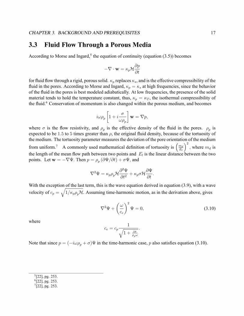
3.3 Fluid Flow Through a Porous MediaAccording to Morse and Ingard,5 the equation of continuity (equation (3.5)) becomes
�r �w = �pH@p
@t
for �uid �ow through a rigid, porous solid. �p replaces �s, and is the effective compressibility of the�uid in the pores. According to Morse and Ingard, �p = �s at high frequencies, since the behaviorof the �uid in the pores is best modeled adiabatically. At low frequencies, the presence of the solidmaterial tends to hold the temperature constant, thus, �p = �T , the isothermal compressibility ofthe �uid.6 Conservation of momentum is also changed within the porous medium, and becomes
i!�p
�1 + i
�
!�p
�w = rp;
where � is the �ow resistivity, and �p is the effective density of the �uid in the pores. �p isexpected to be 1:5 to 5 times greater than �, the original �uid density, because of the tortuosity ofthe medium. The tortuosity parameter measures the deviation of the pore orientation of the mediumfrom uniform.7 A commonly used mathematical de�nition of tortuosity is
�md
El
�2; where md is
the length of the mean �ow path between two points and El is the linear distance between the twopoints. Let w = �r: Then p = �p (@=@t) + �; and
r2 = �p�pH@2
@t2+ �p�H
@
@t:
With the exception of the last term, this is the wave equation derived in equation (3.9), with a wavevelocity of cp =
q1=�p�pH. Assuming time-harmonic motion, as in the derivation above, gives
r2+
�!
ce
�2 = 0; (3.10)
wherece = cp
1q1 + i�
�p!
:
Note that since p = (�i!�p + �) in the time-harmonic case, p also satis�es equation (3.10).
5[22], pg. 253.6[22], pg. 253.7[22], pg. 253.

Chapter 4
The Two Layer Waveguide
The two layer waveguide problem is the simplest model of the soil-air interface (Figure 4.1). Alayer of soil of height zs is bounded by a rigid surface on the bottom, and by the atmosphere onthe top. The partial differential equation governing wave propagation in the soil and air is theHelmholtz Equation, eqn (3.9), which will be solved in cylindrical coordinates.
4.1 Analytical Approach and Separation of VariablesFirst consider the homogeneous problem. Wave propagation through the air and soil, respectively,is described through the following two equations
r2pa + k2apa = 0
r2ps + k2sps = 0;
where ka = !caand ks =
r!2+ i!�
�p
c2s, from substitutions into equations (3.8) and (3.10). Since the
partial differential equations are identical with the exception of the subscripts that determine theappropriate boundary conditions, a "generalized form" of the Helmholtz Equation is used untilboundary conditions with respect to depth are applied. The generalized form of the HelmholtzEquation neglects the difference in acoustic properties between the atmospheric and soil layers,which do not effect the general separation of variables solution with regard to the radial or angularconditions.
r2p+ k2p = 0
Cylindrical coordinates were selected due to the cylindrical features of the membrane problem.1The Helmholtz Equation, rewritten in cylindrical coordinates, is
1
r
@
@r
�r@p
@r
�+1
r2@2p
@�2+@2p
@z2+ k2p = 0
1[16], pg. 2051.
18

CHAPTER 4. THE TWO LAYER WAVEGUIDE 19
Figure 4.1: A mathematical schematic of the two layer waveguide in cylindrical coordinates dis-playing this paper's notation. �a and �s are the density of air and soil, respectively, and ! is theangular frequency imparted from the point source.
Separation of variables, assuming p (r; �; z) = F (r)G (�)Z (z), yields
1
r
@@r(rF 0 (r))
F (r)+1
r2G00 (�)
G (�)= �k2 � Z
00 (z)
Z (z): (4.1)
Equation (4.1) indicates that the two arguments on either side of the equation must equal the sameconstant. This assumption is valid because differentiation of both sides with respect to z impliesthe derivative of Z
00(z)Z(z)
is 0. Therefore, Z00(z)Z(z)
is a constant. This argument works for each variablein equation (4.1). Since sound waves propagate in a way that resembles sinusoidal functions (andnot exponentials), choose �� be an arbitrary constant. Then
�Z00 (z)
Z (z)� k2 = �� (4.2)
and1
r
@@r(rF 0 (r))
F (r)+1
r2G00 (�)
G (�)= ��: (4.3)
Continuing with separation of variables, consider equation (4.3). Multiplication by r2 and rear-ranging yields
r@@r(rF 0 (r))
F (r)+ r2� = �G
00 (�)
G (�): (4.4)

CHAPTER 4. THE TWO LAYER WAVEGUIDE 20
4.1.1 Theta Equation
Equation (4.4) indicates that the two arguments must equal constants, from the same argumentgiven for equation (4.1). Choose � to create sinusoidal functions that will satisfy the periodicityconditions in equation (4.8).
�G00 (�)
G (�)= � (4.5)
r@@r(rF 0 (r))
F (r)+ �r2 = � (4.6)
Equation (4.5) is equal toG00 (�) + �G (�) = 0 (4.7)
Assume � > 0: (� � 0 result in trivial solutions) This assumption is made based on the periodicitycondition implied by the problem con�guration.2 Therefore, solutions are of the form
G (�) = A cos�p���+B sin
�p���
Boundary conditions are now imposed, as described by the periodicity condition below. Thesolution G must therefore satisfy the periodicity conditions
G (��) = G (�) (4.8)
G0 (��) = G0 (�)for continuity at �. After imposing the boundary conditions, the solution becomes
G (�) = A cos (m�) ; (4.9)
with � = m2 wherem = 0; 1; 2; ::
Orthogonality of the Theta Eigenfunctions
Orthogonality is a particularly useful tool in solving partial differential equations. Because orthog-onality will be used in later portions of the mathematical analysis of this problem, it is necessaryto prove the orthogonality of the theta-dependent function, G. By de�nition, a set of functions,f�ng
1n=1 is orthogonal on [0; L] if
R L0�n (x)�m (x) dx = 0, when n 6= m. Using the trigonometric
identity cos (a) cos (b) = 12[cos (a+ b) + cos (a� b)], we obtain thatZ �
��An cos (n�)Am cos (m�) d�
=AnAm2
Z �
��[cos ((n+m) �) + cos ((n�m) �)] d�
2[11], pg. 307.
CHAPTER 4. THE TWO LAYER WAVEGUIDE 21
Performing the integral results in
�nm =
�1 m = n0 m 6= n
�The Kronecker delta function results from An =
q1�in the case where m = n. This selection of
An forms an orthogonal, normalized basis.
4.1.2 Radial ConditionThe radial condition on pressure is established through solving for F (r) (eqn.(4.6))
r@
@r(rF 0 (r)) = ��r2F (r) +m2F (r) :
Rearrangement and multiplication by r2 results in
r2F 00 (r) + rF 0 (r) +��r2 �m2
�F (r) = 0: (4.10)
Let �2 = �r2. Then equation (4.10) becomes a Bessel Differential Equation3
�2 eF 00 (�) + � eF 0 (�) + ��2 �m2� eF (�) = 0:
Solutions to the Bessel Differential Equation are known as Bessel Functions of the �rst and secondkind. Mathematically, these are represented by Jm (�)and Ym (�) : By the principle of super-position, any linear combination of Bessel functions is also a solution to the Bessel DifferentialEquation. One of these combinations is known as a Hankel Function (represented by H(1)
m (�)),which is linear combinations of Bessel Functions of the �rst and second kindeF� (�) = H(1)
m (�) = Jm (�) + iYm (�) (4.11)
eF� (�) = H(2)m (�) = Jm (�)� iYm (�) : (4.12)
4.1.3 Depth EquationWe now consider the z equation, equation (4.2), written in terms of the value of z.(
�Z00a (z)Za(z)
� k2a = �� 0 � z � za�Z00s (z)Zs(z)
� k2s = �� zs � z < 0:
Rearrangement, multiplication by �Z (z) ; and subtraction of (k2 � �) results in�Z 00a (z) + (k
2a � �)Za (z) = 0 0 � z � za
Z 00s (z) + (k2s � �)Zs (z) = 0 zs � z < 0
: (4.13)
3[11], pg. 306.

CHAPTER 4. THE TWO LAYER WAVEGUIDE 22
Suppose k2a > �. Solutions are then of the form
Z (z) =
8<: A cos�p
k2a � �z�+B sin
�pk2a � �z
�0 � z � za
C cos�p
k2s � �z�+D sin
�pk2s � �z
�zs � z < 0
:
As shown in Figure (4.1), there are several boundary conditions that de�ne the solution in the zdirection. First, it is necessary to de�ne an upper limit, za; for the atmosphere when using a pointsource. At and above this limit, the atmosphere is assumed to be a vacuum, that is, the pressure is0. Mathematically, this is written as
p (za) = 0: (4.14)
At the soil-rigid substrate interface, it is expected that some of the energy is re�ected, while someenergy is also absorbed by the rigid substrate. However, the pressure at the interface should beconstant. Therefore,
@
@zp (zs) = 0 (4.15)
At the interface between the atmosphere and soil, (z = 0), the atmospheric pressure should beequal to the acoustic pressure in the soil (Continuity of Pressure).
pa (0) = ps (0) (4.16)
Similarly, at the interface between the atmosphere and soil, the velocity of the acoustic wave shouldbe equal in both the atmosphere and soil. Acoustic impedance relates the �uid velocity to theacoustic pressure.4 Mathematically, acoustic impedance5 is the ratio between acoustic pressure, p,and �uid velocity, represented by the following equation in this problem
�i@@zpa (0)
�a!= �i
@@zps (0)
�s!: (4.17)
Note that this is also continuity of velocity across the air-soil boundary. Equation (4.17) is derivedby assuming time-harmonic oscillations in equation (3.4). Applying the boundary conditions(eqns. (4.14), (4.15), (4.16), and (4.17)) results in
Z (z) =
8<: B1
hcos�p
k2s � �zs�sin�p
k2a � � (za � z)�i
0 � z � zaB1
hsin�p
k2a � �za�cos�p
k2s � � (z � zs)�i
zs � z < 0;
where B1 is an arbitrary constant. From the boundary conditions,24 sin�p
k2a � �za�
cos�p
k2s � �zs�
i
�cos za
pk2a��
�pk2a��
�a!�i
�sin zs
pk2s��
�pk2s��
�s!
35� BD
�=
�00
�:
4[22], pg. 376, 423.5[22], pg. 259.

CHAPTER 4. THE TWO LAYER WAVEGUIDE 23
To ensure that B and D are non-zero, the eigenvalues, �; must force the determinant of the coef�-cient matrix equal to zero. The determinant of the matrix, set equal to zero, is
�spk2a � � cos za
pk2a � � cos zs
pk2s � � (4.18)
+�apk2s � � sin za
pk2a � � sin zs
pk2s � �
= 0:
The solutions to equation (4.18) must be found numerically. A MATLABTM program was writtento solve for the eigenvalues. In order to program this speci�c function into MATLABTM, it wasnecessary to perform a change of variables. This was done so that the eigenvalues would beevenly spaced, and thus, could be found numerically over a long range of values. Therefore, let� = za
pk2a � �. So
� = k2a ���
za
�2and
�s
0@cos (�) cos zssk2s � k2a +
��
za
�21A �
za(4.19)
+�a
0@sin (�) sin zssk2s � k2a +
��
za
�21Ask2s � k2a + � �za�2= 0:
Using MATLABTM and a program for the secant method6, eigenvalues for the depth conditionwere determined.
Air and Soil Eigenvalues
Note that in equation (4.18), �a � �s. Therefore, eigenvalues occur when
cos zapk2a � � cos zs
pk2s � � � 0:
If � is taken to be zapk2a � �, then two sequences of eigenvalues exist; one sequence exists for the
air eigenvalues and another for the soil eigenvalues. The air eigenvalues (�a;n) are given by
�a;n � (2n� 1)�
2;
while the soil eigenvalues (�s;n) are given by
zspk2s � �n = zs
sk2s � k2a +
��s;nza
�2� (2n� 1) �
2;
6[17], pg. 70.

CHAPTER 4. THE TWO LAYER WAVEGUIDE 24
Figure 4.2: This �gure shows the soil and air eigenvalue plots, respectively, for the two-layerwaveguide.
or
�s;n � za
s�(2n� 1) �
2zs
�2� k2s + k2a:
for n 2 N: Resonances occur when �s;n ceases to be evanescent and when �s;n ! 0: Denotethese as E-resonances and Z-resonances. An E-resonance occurs when �s;n = kaza: This resultsin
ks =2�f
cp;s= (2n� 1) �
2 jzsj! f = cp;s
(2n� 1)4 jzsj
:
Similarly, a Z-resonance occurs when �s;n = 0, which gives
fn = (2n� 1)cacs
4 jzsjpc2a � c2s:
The location of the E-resonances and Z-resonances are shown in Figure (4.2). Note that in thisproject, the input values that generated each graph are listed in the appendix.

CHAPTER 4. THE TWO LAYER WAVEGUIDE 25
Figure 4.3: The �rst six eigenvalues for the depth condition. The � values are limited from 0 to20 in this graphic, for demonstration purposes. The zeros of the characteristic function determinethe eigenvalues.
Eigenvalue Plots
Figure (4.3) shows a plot of the characteristic function (eqn. 4.19) at f = 50 Hz. The eigenvaluesin this plot are the E-resonances. Figure (4.3) indicates the �rst of the � eigenvalues occurs atapproximately 2:2, a second eigenvalue of 5:3, and subsequent eigenvalues occurring at intervals ofapproximately �. AMATLABTM program based on the secant method of �nding zeros of a functionwas written, since the secant method converges quickly when the interval containing a zero isknown.7 The eigenvalues depend upon the frequency. Figure (4.4) shows that the eigenvalues arequite sensitive to frequency. Note, however, that the spacing of the values of interest for � remainsat intervals of approximately �. Although there are exceptions to this spacing, the secant methodhas been highly effective in �nding the � which result in zeros of the eigenfunction.
Orthogonality of the Depth Condition
Using a Sturm-Liouville argument, which is outlined in Appendix (A), the eigenfunctions de-scribed in equation (4.18) were con�rmed to be orthogonal. The weight function, as de�ned inAppendix (A), is
� (z) =
��s when 0 < z � za�a when zs � z < 0
7[17], pg. 70.

CHAPTER 4. THE TWO LAYER WAVEGUIDE 26
Figure 4.4: Eigenvalues for the depth condition at multiple frequencies, demonstrating the eigen-function dependence on frequency.
CHAPTER 4. THE TWO LAYER WAVEGUIDE 27
4.2 Insertion of a Point SourceInsertion of a point source, also known as a unit impulse, in the upper waveguide layer leads to theboundary value problem
r2p+ k2p = �1r� (r � r0) � (� � �0) � (z � z0) : (4.20)
The Dirac delta "function", � (x), is a mathematical representation of a function equal to 1 atx = 0, and is equal to 0 for all other values.8 In other words,
� (x� xi) =�0 x 6= xi1 x = xi
(4.21)
Additionally, the delta function has the property that the integral of a function, f (x) ; multipliedby a delta function � (x� x0), over the interval (a; b) (assuming that a � x0 � b)
bRa
f (x) � (x� x0) = f (x0) : (4.22)
Let p (r; �; z) =1Pm=0
1Pn=1
Fmn (r)Gm (�)Zn (z). Then r2p in cylindrical coordinates is repre-
sented by
r2p =1Pm=0
1Pn=1
�F 00mn (r) +
1
rF 0mn (r)
�Gm (�)Zn (z)
�n2
r2Fmn (r)Gm (�)Zn (z) + Fmn (r)Gm (�)
���k2 � �
�Zn (z)
�:
Substitution into eqn (4.20) yields
1Pm=0
1Pn=1
�F 00mn (r) +
1
rF 0mn (r)�
m2
r2Fmn (r) + �nFmn (r)
�Gm (�)Zn (z)
= �1r� (r � r0) � (� � �0) � (z � z0) :
Multiplying by Gk (�)� (z)Zl (z)m; integrating to use the orthogonality of the angular and depthequations, and using the properties of delta functions (eqns. (4.21) and (4.22)) gives�
F 00kl (r) +1
rF 0kl (r)�
m2
r2Fkl (r) + �nFkl (r)
��R��Gk (�)
2 d�zaRzs
� (z)Zl (z)2 dz
= �1r� (r � r0)Gk (�0)� (z0)Zl (z0) :
8[11], pg. 392.

CHAPTER 4. THE TWO LAYER WAVEGUIDE 28
Letting
Ckl =Gk (�0)� (z0)Zl (z0)
�R��Gk (�)
2 d�zaRzs
� (z)Zl (z)2 dz
results inrF 00kl (r) + F
0kl (r) +
�r�n �
m2
r
�Fkl (r) = �Ckl� (r � r0) :
The equation above can be rewritten as
@
@r(rF 0kl (r)) +
�r�n �
m2
r
�Fkl (r) = �Ckl� (r � r0) : (4.23)
and integrating from r0 � " to r0 + " gives
(r0 + ")F0kl (r0 + ")� (r0 � ")F 0kl (r0 � ") +
r0+"Rr0�"
�r�n �
m2
r
�Fkl (r) dr
= �Ckl
Letting "! 0 and requiring that Fkl (r) be continuous at r = r0 gives the conditions
Fkl (r0+) = Fkl (r0�) (4.24)
F 0kl (r0+)� F 0kl (r0�) = �1
r0Ckl
Except at r = r0, equation (4.23) is just Bessel's equation. Thus
Gkl (r) =
�AklJk
�p�lr�; 0 � r < r0
BklH(1)k
�p�lr�; r0 < r
is bounded at the origin and satis�es the Sommerfeld Radiation Condition.9 Bessel functions ofthe �rst kind satisfy boundedness at the origin. The Sommerfeld Radiation Condition states that
limr!1
pr
�@
@rw � ikw
�= 0:
Type 1 Hankel functions satisfy the radiation condition. Additionally, the Hankel function ofthe �rst kind indicates waves propagating outward from the source, which represents the physicalreality. The conditions expressed in (4.24) require
AklJk�p�lr0
��BklH(1)
k
�p�lr0
�= 0
Aklp�lJ
0k
�p�lr0
��Bkl
p�lH
(1)0k
�p�lr0
�= � 1
r0Ckl:
9[25], Ch. 6.32.

CHAPTER 4. THE TWO LAYER WAVEGUIDE 29
Solving for Akl and Bkl results in
Akl = �1r0CklH
(1)k
�p�lr0
��p�lH
(1)0k
�p�lr0
�Jk�p�lr0
�+p�lH
(1)k
�p�lr0
�J 0k�p�lr0
� (4.25)
Bkl = �1r0CklJk
�p�lr0
��p�lH
(1)0k
�p�lr0
�Jk�p�lr0
�+p�lH
(1)k
�p�lr0
�J 0k�p�lr0
� :According to the Handbook of Mathematical Functions10, particularly,
C 0m (z) =�zCm+1 (z) +mCm (z)
z(4.26)
andH(1)k+1 (z)H
(2)k (z)�H(2)
k+1 (z)H(1)k (z) = � 4i
�z; (4.27)
the denominator of equation (4.25) simpli�es to
�p�lH(1)0k
�p�lr0
�Jk�p�lr0
�+p�lH
(1)k
�p�lr0
�J 0k�p�lr0
�= � 2i
�r0:
Thus
Akl = �1r0CklH
(1)k
�p�lr0
�� 2i�r0
= �i�2CklH
(1)k
�p�lr0
�Bkl = �
1r0CklJk
�p�lr0
�� 2i�r0
= �i�2CklJk
�p�lr0
�:
Noting�R��G0 (�)
2 d� = 2�, when G0 (�) = 1
�R��Gm (�)
2 d� = �, when Gm (�) = cos (m�) , sin (m�)
gives
C0n =� (z0)Zn (z0)
2�zaRzs
� (z)Zn (z)2 dz
Cmn =Gm (�0)� (z0)Zn (z0)
�zaRzs
� (z)Zn (z)2 dz
;Gm (�) = cos (m�) , sin (m�) :
10[2], pg. 362, eqn. (9.1.27).

CHAPTER 4. THE TWO LAYER WAVEGUIDE 30
Thus, for r < r0
p (r; �; z) =1Pn=1
� i
4�nH(1)0
�p�nr0
�J0�p�nr�� (z0)Zn (z0)Zn (z) (4.28)
+1Pm=1
1Pn=1
� i
2�n
�H(1)m
�p�nr0
�Jm�p�nr�cos (m�0) cos (m�)
+H(1)m
�p�nr0
�Jm�p�nr�sin (m�0) sin (m�)
�� (z0)Zn (z0)Zn (z)
=1Pn=1
� i
4�nH(1)0
�p�nr0
�J0�p�nr�� (z0)Zn (z0)Zn (z)
+1Pm=1
1Pn=1
� i
2�nH(1)m
�p�nr0
�Jm�p�nr�cos (m (�0 � �))
�� (z0)Zn (z0)Zn (z)
and for r > r0
p (r; �; z) =1Pn=1
� i
4�nH(1)0
�p�nr�J0�p�nr0
�� (z0)Zn (z0)Zn (z) (4.29)
+1Pm=1
1Pn=1
� i
2�nH(1)m
�p�nr�Jm�p�nr0
�cos (m (�0 � �))� (z0)Zn (z0)Zn (z)
where �n =zaRzs
� (z)Zn (z)2 dz.
Velocity in the z-direction is given by
wz = � i
!�(@zp) (4.30)
= � i
!�
� 1Pn=1
� i
4�nH(1)0
�p�nr0
�J0�p�nr�� (z0)Zn (z0)Z
0n (z)
+1Pm=1
1Pn=1
� i
2�nH(1)m
�p�nr0
�Jm�p�nr�cos (m (�0 � �))� (z0)Zn (z0)Z 0n (z)
�
when r < r0, and
wz = � i
!�
� 1Pn=1
� i
4�nH(1)0
�p�nr�J0�p�nr0
�� (z0)Zn (z0)Z
0n (z)
+1Pm=1
1Pn=1
� i
2�nH(1)m
�p�nr�Jm�p�nr0
�cos (m (�0 � �))
�� (z0)Zn (z0)Z 0n (z)]
when r > r0. Note that these results are comparable with similar models found in the literature.11
11[9], [6], [12], [23].

Chapter 5
MATLABTM User Interface for the TwoLayer Waveguide
A user interface, featuring an experimental and laboratory input, was created from the equationsfor the Two Layer Waveguide. Speci�c instructions for the user interface are included, as well asthe theoretical background for the transition of the soil properties to the porous representation.
5.1 Instructions for the Soil Resonance User InterfaceThe soil resonance user interface is designed to aid experimental physicists in predicting soil res-onances in �eld experiments, where equipment is limited, and in laboratory settings, with moreprecisely de�ned measurements and analysis tools. The �eld experiment case ("basic module"),which utilizes atmospheric temperature and humidity and relies on more qualitative measures forsoil type, moisture, and compactness, is designed for rough predictions based on previous data.The laboratory case ("advanced module") uses precise laboratory tests to determine the densityand sound speed through the air and soil.
5.1.1 General Instructions for the User Interface1. Upon obtaining the User Interface �les, save the �les and note their location.
2. Open MATLABTM.
3. In the "Current Directory" script next to the help icon (a yellow ?), select the �le directorywhere the Interface �les are stored.
4. Type "gui" into the "Command Window".
31

CHAPTER 5. MATLABTM USER INTERFACE FOR THE TWO LAYER WAVEGUIDE 32
5.1.2 Instructions for Use of the Basic Module1. To select the basic module, press enter when presented with the advanced selection.
2. Enter the ambient temperature in degrees Celsius.
3. Enter the ambient humidity in decimal form.
4. Select the appropriate soil type which most closely describes the soil in the experiment.Select only the numbers given, decimal values are not acceptable.
5. Approximate the soil moisture on a scale of 1 to 5, with 1 being very dry soil, to 5 beingvery moist soil.
6. Approximate the packing of the soil on a scale of 1 to 4, with 1 being very loose soil, and 4being very compact soil.
5.1.3 Instructions for Use of the Advanced Module1. To select the advanced module, press any number followed by enter when presented with theadvanced selection.
2. Enter the speed of sound in the atmosphere. (Default - 343 m/s). To select the default value,press enter without entering a value. Default values are available for all advanced menuentries. An explanation of the chosen default value follows in the "Theoretical Background"section below.
3. Enter the speed of shear sound waves in the soil. (Default - 210.31 m/s)
4. Enter the speed of compressional sound waves in the soil. (Default - 647 m/s)
5. Enter the �ow resistivity of the soil1. (Default - 0 Pa�sm2 )
6. Enter the density of the atmosphere. (Default - 1.205 kgm3 )
7. Enter the tolerance of the secant method computation. (Default - 5e-5)
5.1.4 General Instructions Following the Basic or Advanced Module1. Enter the depth of the porous soil (above bedrock) AS A NEGATIVE VALUE. For example,if the depth of the soil before hitting bedrock is 0.175 meters, the depth would be entered as"-0.175".
2. Enter the position of the source as a vector. See Figure (5.1) below for further clari�cation.1[3], pg. 175.

CHAPTER 5. MATLABTM USER INTERFACE FOR THE TWO LAYER WAVEGUIDE 33
Figure 5.1: The physical representation of the numerical entry quantities for source and positionof the two-layer waveguide user interface.
3. If interested in a frequency - pressure plot, enter the range of frequencies of interest as avector (ie, if a frequency sweep from 100-200 is desired, enter [100,200]. If a depth -pressure plot is of interest, press enter. Then enter the depth range of interest (in the sameformat as the frequency sweep), press enter and enter the frequency of interest.
5.2 Theoretical BackgroundThe theoretical background necessary to write the programs devised for the numerical implemen-tation is described in this section. The background presented here is applicable for the numericalimplementation shown throughout this paper.
5.2.1 The Basic ModuleThe ambient temperature is used to approximate the density of the air and the sound speed throughthe air. Density was determined using data from E. Sengpiel2, and sound speed was found usingthe formula3
ca;T = 331:4 + 0:6� Tamb�0C�:
2[24]3[24]

CHAPTER 5. MATLABTM USER INTERFACE FOR THE TWO LAYER WAVEGUIDE 34
Figure 5.2: This table shows the user interface soil labels with the soil labels from the originalpaper by Oelze et al6.
Humidity also affects sound speed and density. The atmospheric density was adjusted by
�a = �a;T (1 +H)=(1 + 1:609H);4
where �a;T is the density from the temperature data, andH is the humidity percentage. The soundspeed through the air is determined from
ca = ca;T + 0:6Hca;T :5
The soil type and composition entries are compared to data collected by Oelze et al.6 The soillabels are contained in table (5.2). The exact percentage of composition is also available in theOelze paper.7
5.2.2 The Advanced ModuleThe default values for density and speed in each medium are from data collected by Dr. D. KeithWilson and Dr. H. Cudney in a dry, desert - like environment. The default � = 0 was chosen forsimplicity. Finally, the tolerance for the secant method is a reasonable value for the data.
4[26]5[24]6[8], pg. 792.7[8], pg. 789.

Chapter 6
Numerical Analysis of the Two LayerWaveguide Problem
A MATLABTM program was devised to calculate the pressure and velocity described in equations(4.28) and (4.30). The program and its supporting commands can be found in the appendix. Therewere many reasons behind writing the program for the simple, two layer waveguide problem. Theprogramwill provide the basic structure for future programs involving more complicated problems,and will allow the development of solutions to anticipated problems. Additionally, the effects ofnumerical selection for the atmospheric height (za) and rigid soil depth (zs) need to be investigatedto analyze their contribution to the pressure and velocity. Assumptions for the variables for eachgraphic are as follows (unless otherwise stated): � = 0; cs = 160; ca = 330; zs = �1; za = 500:The value for � was chosen for simplicity, cs, ca and zs are appropriate for the environment ofinterest, and za was computationally determined.
6.1 Determining Resonances for the Two LayerWaveguide Prob-lem
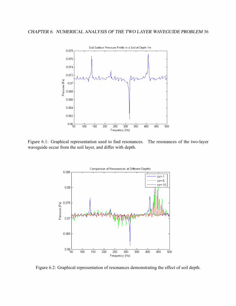
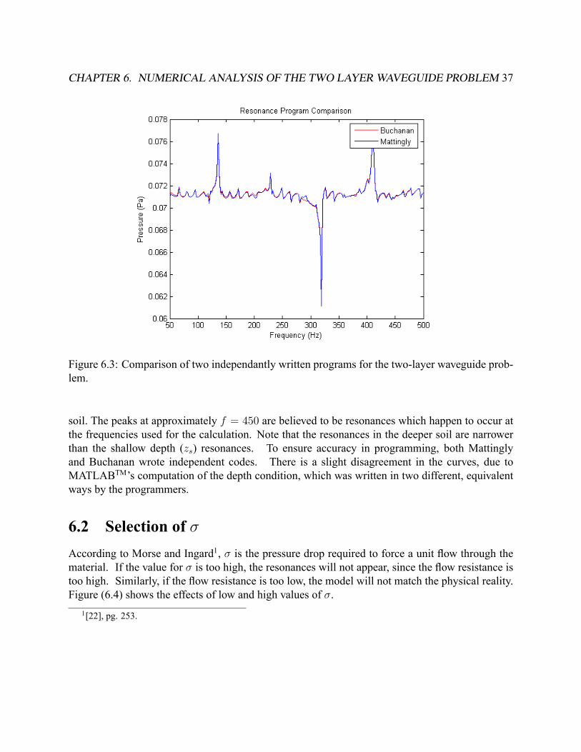
Equation (4.28) describes the pressure at a point (r; �; z). Resonant frequencies, or resonances,are the frequencies at which there are large amplitude oscillations. Thus, resonances are indicatedby large deviations in pressure caused by the acoustic wave. Resonances in Figure (6.1) occur atf � 136; 228; 319; 412Hz. In context of the two layer waveguide problem, resonances indicate thatthe soil surface oscillates at maximum amplitude at these frequencies. The direction of the peak(up or down) is not signi�cant, it is connected to constructive and destructive interference. Shouldlandmine detection be attempted at low soil depths (before hitting bedrock), Figure (6.1) suggeststhat resonances detected in the range of f � 136; 228; 319; 412 Hz are probably soil resonances,instead of mine resonances. Figure (6.2) compares the effect of deeper soil on resonant effects ofthe rigid substrate. It is reasonable that resonances existing at a depth of 1 meter would not beas apparent or appear at all in deeper soil, due to greater attenuation with distance. In fact, thereare more resonances in deeper soil, but these resonances occur at broader frequencies in shallow
35
CHAPTER 6. NUMERICAL ANALYSIS OF THE TWO LAYER WAVEGUIDE PROBLEM 36
Figure 6.1: Graphical representation used to �nd resonances. The resonances of the two-layerwaveguide occur from the soil layer, and differ with depth.
Figure 6.2: Graphical representation of resonances demonstrating the effect of soil depth.
CHAPTER 6. NUMERICAL ANALYSIS OF THE TWO LAYER WAVEGUIDE PROBLEM 37
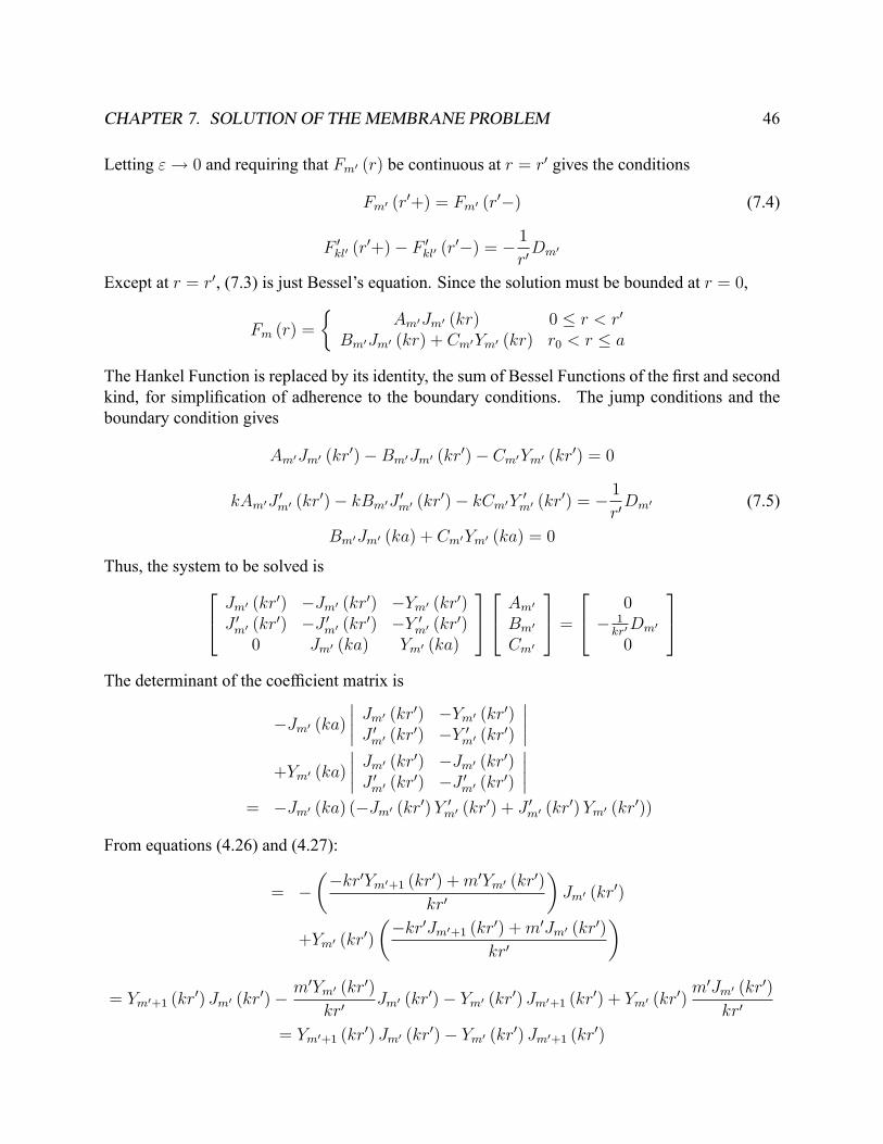
Figure 6.3: Comparison of two independantly written programs for the two-layer waveguide prob-lem.
soil. The peaks at approximately f = 450 are believed to be resonances which happen to occur atthe frequencies used for the calculation. Note that the resonances in the deeper soil are narrowerthan the shallow depth (zs) resonances. To ensure accuracy in programming, both Mattinglyand Buchanan wrote independent codes. There is a slight disagreement in the curves, due toMATLABTM's computation of the depth condition, which was written in two different, equivalentways by the programmers.
6.2 Selection of �According to Morse and Ingard1, � is the pressure drop required to force a unit �ow through thematerial. If the value for � is too high, the resonances will not appear, since the �ow resistance istoo high. Similarly, if the �ow resistance is too low, the model will not match the physical reality.Figure (6.4) shows the effects of low and high values of �.
1[22], pg. 253.

CHAPTER 6. NUMERICAL ANALYSIS OF THE TWO LAYER WAVEGUIDE PROBLEM 38
Figure 6.4: This graph demonstrates the effect of � on pressure. Note that resonances do notappear when � is very high.
6.3 Selection of zaThe effects of the numerical selection for the atmospheric height (za) were considered. The ap-propriate value for za will not show signi�cant deviation from much larger values, and its behaviorwill be consistent with the larger values. za needs to be as small as possible to maximize thecomputational ef�ciency of the program. The receiver height versus pressure graph, Figure (6.5),allows comparison of the different values for za. After investigation, an appropriate value for zais 500 meters. The pressures recorded at 500 meters closely resemble the pressures recorded at800 meters over the span of 100 hertz, as shown in Figure (6.6). Lower values for za, as showin Figure (6.5), show noticeable deviation from za = 500 m. For example, the next lower valueof za = 200 m (in red) does not closely resemble the behavior of za = 800 m, particularly at theresonant frequency, f = 128 Hz.
6.4 Effects of zsThe considerations for the depth of the soil is entirely dependent on the operating environment.The rigid soil depth physically represents the depth at which the porous soil layer interfaces witha more dense (bedrock-type) soil that re�ects most of the acoustic energy. This soil depth isalso dependant on soil type. In Figure (6.7), a dry soil environment, the resonant effects are verydistinguished when compared to Figure (6.8), a moist soil environment. The effects of moisture

CHAPTER 6. NUMERICAL ANALYSIS OF THE TWO LAYER WAVEGUIDE PROBLEM 39
Figure 6.5: Graphical representation of the effect of za on the pressure placed on the mine. Theoptimal value for za will approximate za at much larger values, while remaining computationallyef�cient.
Figure 6.6: Graphical representation of the effect of za on the pressure at z = 0. This graphicshows the comparison for the hypothesized optimal value for za (500m), approximating za at muchlarger values (800 m).

CHAPTER 6. NUMERICAL ANALYSIS OF THE TWO LAYER WAVEGUIDE PROBLEM 40
Figure 6.7: Graphical representation of the effect of zs on the pressure placed on the mine. Thisgraphic shows the comparison for depth of the bedrock layers in a sandy soil environment.
are incorporated into the soil sound speed, cs.2 Smaller pressures are recorded in the moist soilenvironment, and the resonances are barely distinguishable. This mathematical �nding makesphysical sense: a moist soil is more dense, causing more attenuation in the sound wave, whichresults in lower pressure differences and decreased resonant effects. � remained at zero for thecomputation presented below, but future analysis of different soils will need to include different�, which is clearly effected by soil type. Values suggested in a soil sound speed paper3 are beingexamined for their relevance to this problem.
2[8], pg. 792.3[8], pg. 792.

CHAPTER 6. NUMERICAL ANALYSIS OF THE TWO LAYER WAVEGUIDE PROBLEM 41
Figure 6.8: Graphical representation of the effect of zs on the acoustic pressure. This graphicshows the comparison for depth of the bedrock layers in a mixed soil environment. (The compu-tations in this graphic considered only a change in sound speed, since the values for � have yet tobe validated.

Chapter 7
Solution of the Membrane Problem
Figure (7.1) represents the membrane problem, which consists of the top plate of the landmineimbedded in the rigid substrate from the waveguide of the two layer waveguide problem. While thefunctions outside the imaginary cylinder remain identical to those from the two layer waveguideproblem (see eqns. (4.28) and (4.29)), the equations within the cylinder will be derived in thefollowing 2 chapters.
7.1 De�nition of the Green's FunctionSuppose now that a membrane occupies the region D = f(r; �) : r � ag. The equation for themotion of a damped membrane subject to an external pressure p (r; �; t) is
Tr2u� �@tu+ p = �@ttu:
where T is the tension of the membrane and � is its density. If the external pressure is time-harmonic p (r; �; t) = p (r; �) e�i!t and the membrane is �xed at the boundary, then
r2u+ k2u = � 1Tp
u (a; �) = 0
with k2 = (�!2 + i�!) =T . Let G (r; �; r0; �0) denote the Green's function for the problem, that is,
r2(r;�)G + k2G = �
1
r� (r � r0) � (� � �0) (7.1)
G (a; �; r0; �0) = 0;G (r; �; r0; �0) = G (r0; �0; r; �)
42

CHAPTER 7. SOLUTION OF THE MEMBRANE PROBLEM 43
Figure 7.1: A mathematical schematic of the membrane problem in cylindrical coordinates dis-playing this paper's notation. T is the tension of the membrane, which will be examined for thecase of the plastic landmine.

CHAPTER 7. SOLUTION OF THE MEMBRANE PROBLEM 44
Note thataR0
�R��
�G (r; �; r0; �0)r2u (r; �)� ur2
(r;�)G (r; �; r0; �0)�rd�dr
=aR0
�R��
��G (r; �; r0; �0)
�k2u (r; �) +
1
Tp (r; �)
�+
�k2G (r; �; r0; �0) + 1
r� (r � r0) � (� � �0)
�u (r; �)
�rd�dr
= � 1T
aR0
�R��G (r; �; r0; �0) p (r; �) rd�dr + u (r0; �0) :
Since r � (urv) = ru � rv + ur2v, the divergence theorem givesaR0
�R��
�G (r; �; r0; �0)r2u (r; �)� ur2
(r;�)G (r; �; r0; �0)�rd�dr
=RRD
[r � (Gru)�rG � ru� (r � (urG �rG � ru))] dA
=
Z@D
[Gru � n� urG � n] ds = 0
in view of the boundary conditions. Thus, the solution to the non-homogeneous membrane prob-lem is
u (r; �) =1
T
aR0
�R��G (r; �; r0; �0) p (r0; �0) r0d�0dr0 (7.2)
7.2 Determination of the Green's FunctionIt remains to �nd the Green's function. In polar coordinates,
1
r@r (r@rG) +
1
r2@��G + k2G = 0
except at (r; �) = (r0; �0). Seeking solutions of the form �(r; �) = F (r)G (�) gives
1r(rF 0 (r))0
F (r)+1
r2G00 (�)
G (�)+ k2 = 0
�r (rF0 (r))0
F (r)� k2r2 = G00 (�)
G (�)= ��
From equations (4.7) and (4.8) the problem
G00 (�) + �G (�) = 0
G (��) = G (�) ; G0 (��) = G0 (�)

CHAPTER 7. SOLUTION OF THE MEMBRANE PROBLEM 45
has the solution�m = m
2;m = 0; 1; 2; :::
G0 = 1; Gm (�) = cos (m�) ; sin (m�) :
The problem for F (r) isr (rF 0 (r))
0+�k2r2 �m2
�F (r) = 0
F (a) = 0
Substituting a solution of the form G (r; �) =P1
m=0 Fm (r)Gm (�) into the Laplacian gives
1
r@r (r@rG) +
1
r2@��G
=1Xm=0
1
r
d
dr(rF 0m (r))Gm (�) +
1
r2Fm (r)G
00m (�)
=1Xm=0
�F 00m (r) +
1
rF 0m (r)
�Gm (�)�
m2
r2Fm (r)Gm (�)
Substituting this into (7.1) gives1Xm=0
�F 00m (r) +
1
rF 0m (r)
�Gm (�)�
m2
r2Fm (r)Gm (�) + k
2Fm (r)Gm (�)
= �1r� (r � r0) � (� � �0)
1Xm=0
�rF 00m (r) + F
0m (r) +
�k2r � m
2
r
�Fm (r)
�Gm (�) = �� (r � r0) � (� � �0)
Multiplying by Gm0 (�) and integrating gives�rF 00m0 (r) + F 0m0 (r) +
�k2r � m
02
r
�Fm0 (r)
��R��Gm0 (�)2 d�
= �� (r � r0)Gm0 (�0)
rF 00m0 (r) + F 0m0 (r) +
�k2r � m
02
r
�Fm0 (r) = �Dm0� (r � r0) (7.3)
whereDm0 =
Gm0 (�0)�R��Gm0 (�0)
2d�
:
Integrating from r0 � " to r0 + " gives
(r0 + ")F 0m0 (r0 + ")� (r0 � ")F 0m0 (r0 � ") +Z r0+"
r0�"
�k2r � m
02
r
�Fm0 (r) dr
= �Dm0
CHAPTER 7. SOLUTION OF THE MEMBRANE PROBLEM 46
Letting "! 0 and requiring that Fm0 (r) be continuous at r = r0 gives the conditions
Fm0 (r0+) = Fm0 (r0�) (7.4)
F 0kl0 (r0+)� F 0kl0 (r0�) = �
1
r0Dm0
Except at r = r0, (7.3) is just Bessel's equation. Since the solution must be bounded at r = 0,
Fm (r) =
�Am0Jm0 (kr) 0 � r < r0
Bm0Jm0 (kr) + Cm0Ym0 (kr) r0 < r � a
The Hankel Function is replaced by its identity, the sum of Bessel Functions of the �rst and secondkind, for simpli�cation of adherence to the boundary conditions. The jump conditions and theboundary condition gives
Am0Jm0 (kr0)�Bm0Jm0 (kr0)� Cm0Ym0 (kr0) = 0
kAm0J 0m0 (kr0)� kBm0J 0m0 (kr0)� kCm0Y 0m0 (kr0) = �1
r0Dm0 (7.5)
Bm0Jm0 (ka) + Cm0Ym0 (ka) = 0
Thus, the system to be solved is24 Jm0 (kr0) �Jm0 (kr0) �Ym0 (kr0)J 0m0 (kr0) �J 0m0 (kr0) �Y 0m0 (kr0)
0 Jm0 (ka) Ym0 (ka)
3524 Am0
Bm0
Cm0
35 =24 0� 1kr0Dm0
0
35The determinant of the coef�cient matrix is
�Jm0 (ka)
���� Jm0 (kr0) �Ym0 (kr0)J 0m0 (kr0) �Y 0m0 (kr0)
����+Ym0 (ka)
���� Jm0 (kr0) �Jm0 (kr0)J 0m0 (kr0) �J 0m0 (kr0)
����= �Jm0 (ka) (�Jm0 (kr0)Y 0m0 (kr0) + J 0m0 (kr0)Ym0 (kr0))
From equations (4.26) and (4.27):
= ���kr0Ym0+1 (kr
0) +m0Ym0 (kr0)
kr0
�Jm0 (kr0)
+Ym0 (kr0)
��kr0Jm0+1 (kr
0) +m0Jm0 (kr0)
kr0
�
= Ym0+1 (kr0) Jm0 (kr0)� m
0Ym0 (kr0)
kr0Jm0 (kr0)� Ym0 (kr0) Jm0+1 (kr
0) + Ym0 (kr0)m0Jm0 (kr0)
kr0
= Ym0+1 (kr0) Jm0 (kr0)� Ym0 (kr0) Jm0+1 (kr
0)
CHAPTER 7. SOLUTION OF THE MEMBRANE PROBLEM 47
By Abramowitz and Stegun1
J�+1 (z)Yv (z)� J� (z)Yv+1 (z) = �2
� (z)
so our equation yields:= � 2
� (kr0)
Thus, by Cramer's Rule
Am0 = � � (kr0)
2Jm0 (ka)
������0 �Jm0 (kr0) �Ym0 (kr0)
� 1kr0Dm0 �J 0m0 (kr0) �Y 0m0 (kr0)0 Jm0 (ka) Ym0 (ka)
������= �
�� � (kr0)
2Jm0 (ka)
�� 1
kr0Dm0
� ���� �Jm0 (kr0) �Ym0 (kr0)Jm0 (ka) Ym0 (ka)
�����= � � (kr0)
2Jm0 (ka)
�1
kr0Dm0
�(�Jm0 (kr0)Ym0 (ka) + Ym0 (kr0) Jm0 (ka))
= � �
2Jm0 (ka)(Dm0) (�Jm0 (kr0)Ym0 (ka) + Ym0 (kr0) Jm0 (ka))
Similarly,
Bm0 = � � (kr0)
2Jm0 (ka)
������Jm0 (kr0) 0 �Ym0 (kr0)J 0m0 (kr0) � 1
kr0Dm0 �Y 0m0 (kr0)0 0 Ym0 (ka)
������=
�
2Jm0 (ka)Dm0Jm0 (kr0)Ym0 (ka)
Cm0 = � � (kr0)
2Jm0 (ka)
������Jm0 (kr0) �Jm0 (kr0) 0J 0m0 (kr0) �J 0m0 (kr0) � 1
kr0Dm0
0 Jm0 (ka) 0
������= � �
2Jm0 (ka)Dm0Jm0 (kr0) Jm0 (ka) = ��
2Dm0Jm0 (kr0)
Noting that
D0 =G0 (�
0)�R��G0 (�
0)2d�
=1
2�
Dm =Gm (�
0)�R��Gm (�
0)2d�
=Gm (�
0)
�;Gm (�
0) = cos (�0) ; sin (�0)
1[2], pg. 362, eqn. (9.1.16).
CHAPTER 7. SOLUTION OF THE MEMBRANE PROBLEM 48
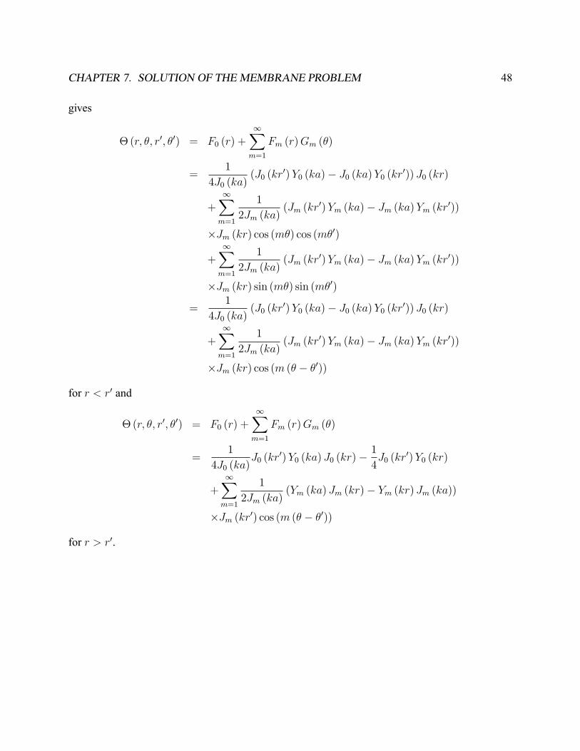
gives
�(r; �; r0; �0) = F0 (r) +
1Xm=1
Fm (r)Gm (�)
=1
4J0 (ka)(J0 (kr
0)Y0 (ka)� J0 (ka)Y0 (kr0)) J0 (kr)
+
1Xm=1
1
2Jm (ka)(Jm (kr
0)Ym (ka)� Jm (ka)Ym (kr0))
�Jm (kr) cos (m�) cos (m�0)
+1Xm=1
1
2Jm (ka)(Jm (kr
0)Ym (ka)� Jm (ka)Ym (kr0))
�Jm (kr) sin (m�) sin (m�0)
=1
4J0 (ka)(J0 (kr
0)Y0 (ka)� J0 (ka)Y0 (kr0)) J0 (kr)
+1Xm=1
1
2Jm (ka)(Jm (kr
0)Ym (ka)� Jm (ka)Ym (kr0))
�Jm (kr) cos (m (� � �0))
for r < r0 and
�(r; �; r0; �0) = F0 (r) +1Xm=1
Fm (r)Gm (�)
=1
4J0 (ka)J0 (kr
0)Y0 (ka) J0 (kr)�1
4J0 (kr
0)Y0 (kr)
+1Xm=1
1
2Jm (ka)(Ym (ka) Jm (kr)� Ym (kr) Jm (ka))
�Jm (kr0) cos (m (� � �0))
for r > r0.
CHAPTER 7. SOLUTION OF THE MEMBRANE PROBLEM 49
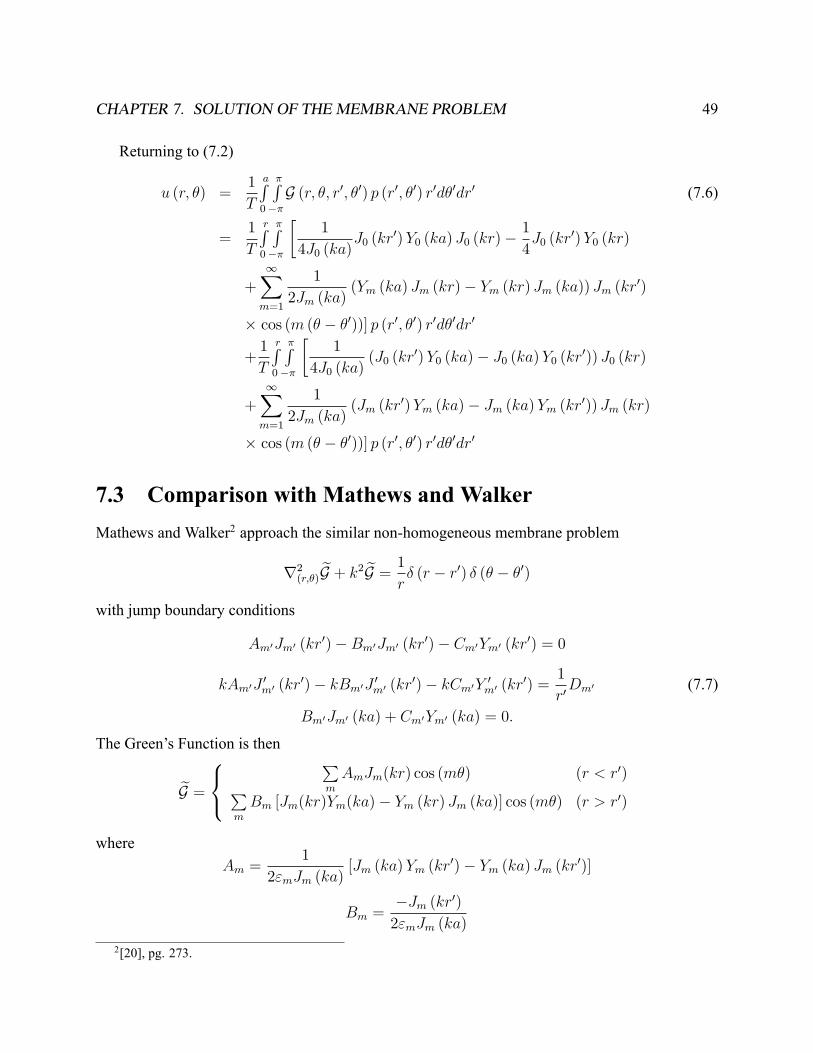
Returning to (7.2)
u (r; �) =1
T
aR0
�R��G (r; �; r0; �0) p (r0; �0) r0d�0dr0 (7.6)
=1
T
rR0
�R��
�1
4J0 (ka)J0 (kr
0)Y0 (ka) J0 (kr)�1
4J0 (kr
0)Y0 (kr)
+1Xm=1
1
2Jm (ka)(Ym (ka) Jm (kr)� Ym (kr) Jm (ka)) Jm (kr0)
� cos (m (� � �0))] p (r0; �0) r0d�0dr0
+1
T
rR0
�R��
�1
4J0 (ka)(J0 (kr
0)Y0 (ka)� J0 (ka)Y0 (kr0)) J0 (kr)
+1Xm=1
1
2Jm (ka)(Jm (kr
0)Ym (ka)� Jm (ka)Ym (kr0)) Jm (kr)
� cos (m (� � �0))] p (r0; �0) r0d�0dr0
7.3 Comparison with Mathews and WalkerMathews and Walker2 approach the similar non-homogeneous membrane problem
r2(r;�)
eG + k2 eG = 1
r� (r � r0) � (� � �0)
with jump boundary conditions
Am0Jm0 (kr0)�Bm0Jm0 (kr0)� Cm0Ym0 (kr0) = 0
kAm0J 0m0 (kr0)� kBm0J 0m0 (kr0)� kCm0Y 0m0 (kr0) =1
r0Dm0 (7.7)
Bm0Jm0 (ka) + Cm0Ym0 (ka) = 0:
The Green's Function is then
eG =8<:
Pm
AmJm(kr) cos (m�) (r < r0)Pm
Bm [Jm(kr)Ym(ka)� Ym (kr) Jm (ka)] cos (m�) (r > r0)
whereAm =
1
2"mJm (ka)[Jm (ka)Ym (kr
0)� Ym (ka) Jm (kr0)]
Bm =�Jm (kr0)2"mJm (ka)
2[20], pg. 273.

CHAPTER 7. SOLUTION OF THE MEMBRANE PROBLEM 50
and"m =
�2 ifm0 = 01 ifm0 > 0
Therefore, for r < r0,
eG =Pm
AmJm(kr) cos (m�)
=1
4J0 (ka)[J0 (ka)Y0 (kr
0)� Y0 (ka) J0 (kr0)] J0(kr)
+Pm
1
2Jm (ka)[Jm (ka)Ym (kr
0)� Ym (ka) Jm (kr0)]
�Jm(kr) cos (m�)
while for r > r0,
eG =Pm
Bm [Jm(kr)Ym(ka)� Ym (kr) Jm (ka)] cos (m�)
=�J0 (kr0)4J0 (ka)
[J0(kr)Y0(ka)� Y0 (kr) J0 (ka)]
+Pm
�Jm (kr0)2Jm (ka)
[Jm(kr)Ym(ka)� Ym (kr) Jm (ka)] cos (m�)
The solution in Mathews and Walker is identical to the solution presented in this paper, with theexception of a negative sign in each portion (due to the absence of the negative sign preceding 1
r0 inequation (7.7)).
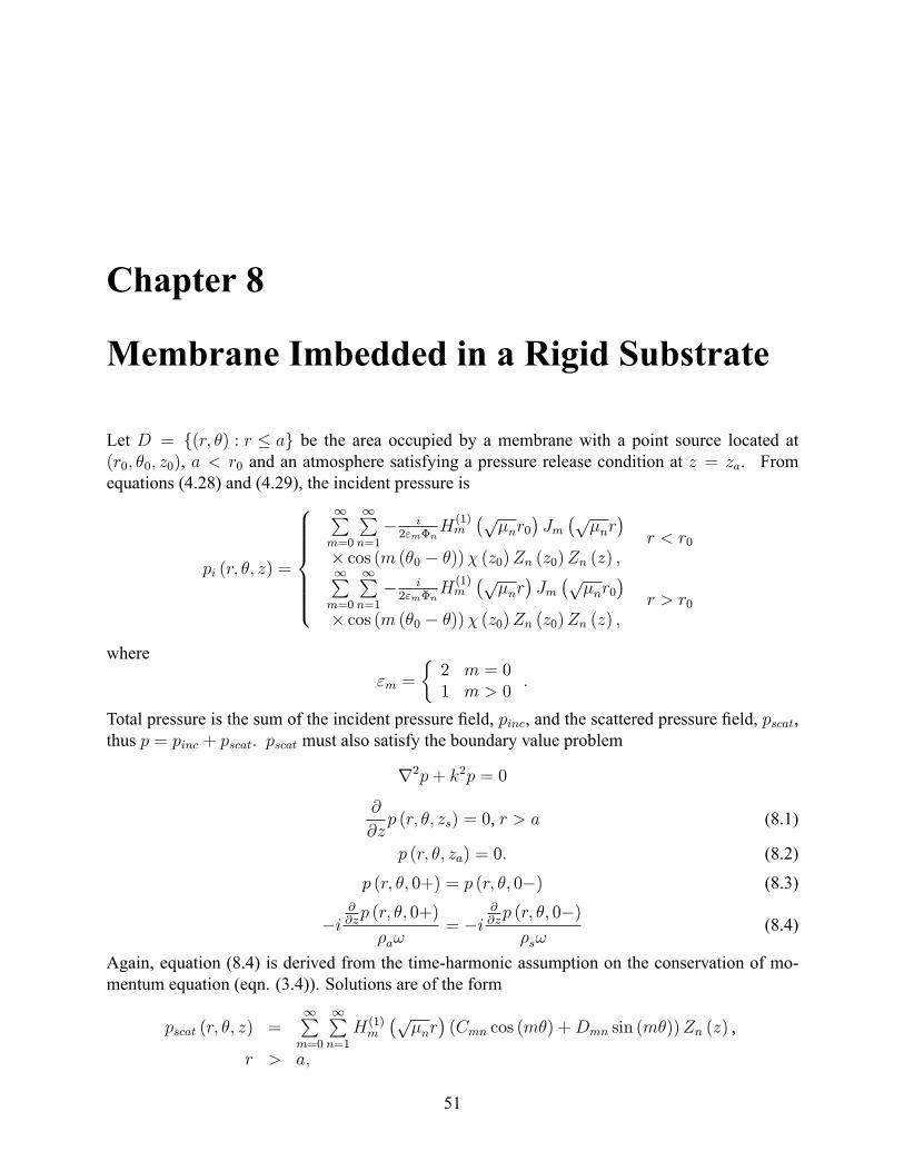
Chapter 8
Membrane Imbedded in a Rigid Substrate
Let D = f(r; �) : r � ag be the area occupied by a membrane with a point source located at(r0; �0; z0), a < r0 and an atmosphere satisfying a pressure release condition at z = za. Fromequations (4.28) and (4.29), the incident pressure is
pi (r; �; z) =
8>>>>><>>>>>:
1Pm=0
1Pn=1
� i2"m�n
H(1)m
�p�nr0
�Jm�p�nr�
� cos (m (�0 � �))� (z0)Zn (z0)Zn (z) ;r < r0
1Pm=0
1Pn=1
� i2"m�n
H(1)m
�p�nr�Jm�p�nr0
�� cos (m (�0 � �))� (z0)Zn (z0)Zn (z) ;
r > r0
where"m =
�2 m = 01 m > 0
:
Total pressure is the sum of the incident pressure �eld, pinc, and the scattered pressure �eld, pscat,thus p = pinc + pscat: pscat must also satisfy the boundary value problem
r2p+ k2p = 0
@
@zp (r; �; zs) = 0, r > a (8.1)
p (r; �; za) = 0: (8.2)
p (r; �; 0+) = p (r; �; 0�) (8.3)
�i@@zp (r; �; 0+)
�a!= �i
@@zp (r; �; 0�)�s!
(8.4)
Again, equation (8.4) is derived from the time-harmonic assumption on the conservation of mo-mentum equation (eqn. (3.4)). Solutions are of the form
pscat (r; �; z) =1Pm=0
1Pn=1
H(1)m
�p�nr�(Cmn cos (m�) +Dmn sin (m�))Zn (z) ,
r > a;
51

CHAPTER 8. MEMBRANE IMBEDDED IN A RIGID SUBSTRATE 52
where �n are the eigenvalues from Problem two layer waveguide (eqn. 4.18). Above the mem-brane, total pressure is given by
p (r; �; z) =1Pm=0
1Pn=1
Jm
�p�mnr
�(Amn cos (m�) +Bmn sin (m�))�mn (z) , (8.5)
r < a;
where the eigenvalues �mn and the eigenfunctions �mn (z) are to be determined.At the interface r = a the continuity conditions
pscat (a+; �; z) + pinc (a+; �; z) = p (a�; �; z) (8.6)
@rpscat (a+; �; z) + @rpinc (a+; �; z) = @rp (a�; �; z)are imposed. At z = zs continuity of velocity gives, in the case of the time-harmonic oscillations,
�i!u (r; �) = 1
i!�s@zp (r; �; zs) ; r < a (8.7)
where u is the vertical displacement of the membrane and �s is the density of the soil.
8.1 Solution of the Problem
8.1.1 The Eigenvalue ProblemThe eigenfunctions in the atmosphere �mn;a (z) satisfy the equations
�00mn;a (z) +�k2a � �
��mn;a (z) = 0
�mn;a (za) = 0
The differential equation has solution
�mn;a (z) = E cos (az) + F sin (az) ;
where2a = k
2a � �:
The pressure release condition (eqn. (8.2)) gives
E cos (aza) + F sin (aza) = 0
E cos (aza) = �F sin (aza) :Note that �mn;a (z) becomes E1 sin (a (z � za)) for some E1. The eigenfunctions in the soilsatisfy the equations
�00mn;s (z) +�k2s � �
��mn;s (z) = 0

CHAPTER 8. MEMBRANE IMBEDDED IN A RIGID SUBSTRATE 53
The differential equation has solution
�mn;s (z) = K cos (sz) + L sin (sz) ;
where2s = k
2s � �:
Note that equation (8.1) does not apply, since for �mn;s, r � a:The atmosphere-soil interfacecondition (eqn. (8.3)) on pressure implies
�E1 sin (a (za)) = Kand continuity of velocity (eqn. (8.4)) gives
�ia (cos (aza))�a!
= �isL�s!
Substitution into �mn;a (z) yields
�mn;a (z) = E1 sin (a (z � za))and �mn;s (z) is
�mn;s (z) = E1
��sa�as
cos (aza) sin (sz)� sin (aza) cos (sz)�
Thus, the eigenfunctions have the form
�mn (z) =
�sin (a (z � za)) 0 � z � za
�sa�as
cos (aza) sin (sz)� sin (a (za)) cos (sz) zs � z < 0:
From (7.6) the response of the membrane to an external pressure, pe; is
u (r; �) =1
2T
rR0
�R��
1Xm=0
1
"mJm (ka)(Ym (ka) Jm (kr)� Ym (kr) Jm (ka)) (8.8)
�Jm (kr0) cos (m (� � �0)) pe (r0; �0) r0d�0dr0
+1
2T
aRr
�R��
1Xm=0
1
"mJm (ka)(Jm (kr
0)Ym (ka)� Jm (ka)Ym (kr0))
�Jm (kr) cos (m (� � �0)) pe (r0; �0) r0d�0dr0
=1
2T
1Xm=0
1
"mJm (ka)(Ym (ka) Jm (kr)� Ym (kr) Jm (ka))
�rR0
Jm (kr0)
�R��cos (m (� � �0)) pe (r0; �0) d�0r0dr0
+1
2T
1Xm=0
Jm (kr)
"mJm (ka)
aRr
(Jm (kr0)Ym (ka)� Jm (ka)Ym (kr0))
��R��cos (m (� � �0)) pe (r0; �0) d�0r0dr0:

CHAPTER 8. MEMBRANE IMBEDDED IN A RIGID SUBSTRATE 54
Since in this problem pe (r0; �0) = p (r0; �0; zs) where p is given by (8.5),�R��cos (m (� � �0)) pe (r0; �0) d�0
=�R��
1Pm0=0
1Pn=1
Jm0
�p�mnr
0�(Am0n cos (m
0�0) +Bm0n sin (m0�0))
��mn (zs) cos (m (� � �0)) d�0
= "m�1Pn=1
Jm
�p�mnr
0�(Amn cos (m�) +Bmn sin (m�))
��cos (aza) cos (szs)�
�sa�as
sin (aza) sin (szs)
�in which case equation (8.8) becomes
u (r; �) =�
2T
1Xm=0
1Xn=1
1
Jm (ka)(Ym (ka) Jm (kr)� Ym (kr) Jm (ka))
� (Amn cos (m�) +Bmn sin (m�))rR0
Jm (kr0) Jm
�p�mnr
0�r0dr0
���sa�as
cos (aza) sin (szs)� sin (aza) cos (szs)�
+�
2T
1Xm=0
1Xn=1
Jm (kr)
Jm (ka)(Amn cos (m�) +Bmn sin (m�))
�aRr
(Jm (kr0)Ym (ka)� Jm (ka)Ym (kr0)) Jm
�p�mnr
0�r0dr0
���sa�as
cos (aza) sin (szs)� sin (aza) cos (szs)�
According to MAPLETM
(Ym (ka) Jm (kr)� Ym (kr) Jm (ka))rR0
Jm (kr0) Jm
�p�mnr
0�r0dr0
+Jm (kr)aRr
(Jm (kr0)Ym (ka)� Jm (ka)Ym (kr0)) Jm
�p�mnr
0�r0dr0
=k
k2 � �mn
�rJm (ka) Jm
�p�mnr
�[Jm (kr)Ym+1 (kr)� Jm+1 (kr)Ym (kr)]
+aJm (kr) Jm�p�mna
�[Jm+1 (ka)Ym (ka)� Jm (ka)Ym+1 (ka)]
�=
2
� (k2 � �mn)
�Jm (kr) Jm
�p�mna
�� Jm (ka) Jm
�p�mnr
��where the identity1
Jm+1 (z)Ym (z)� Jm (z)Ym+1 (z) =2
�z1[2], pg. 362, eqn. (9.1.16).

CHAPTER 8. MEMBRANE IMBEDDED IN A RIGID SUBSTRATE 55
has been used. Thus,
u (r; �) =1
T
1Xm=0
1Xn=1
1
(k2 � �mn) Jm (ka)(Amn cos (m�) +Bmn sin (m�))
��Jm (kr) Jm
�p�mna
�� Jm (ka) Jm
�p�mnr
�����sa�as
cos (aza) sin (szs)� sin (aza) cos (szs)�
and from equation (8.5)
@zp (r; �; zs) =1Pm=0
1Pn=1
Jm
�p�mnr
�(Amn cos (m�) +Bmn sin (m�))
���sa�a
cos (aza) cos (szs) + s sin (aza) sin (szs)
�and equation (8.7) becomes
�s!2
T
1Xm=0
1Xn=1
1
(k2 � �mn) Jm (ka)(Amn cos (m�) +Bmn sin (m�))
��Jm (kr) Jm
�p�mna
�� Jm (ka) Jm
�p�mnr
�����sa�as
cos (aza) sin (szs)� sin (aza) cos (szs)�
=1Pm=0
1Pn=1
Jm
�p�mnr
�(Amn cos (m�) +Bmn sin (m�))
���sa�a
cos (aza) cos (szs) + s sin (aza) sin (szs)
�:
Equating the coef�cients of the trigonometric functions gives
�a!2
T
1Xn=1
1
(k2 � �mn) Jm (ka)
�Amn�Jm (kr) Jm
�p�mna
�� Jm (ka) Jm
�p�mnr
�����sa�as
cos (aza) sin (szs)� sin (aza) cos (szs)�
=1Pn=1
Jm
�p�mnr
�Amn
���sa�a
cos (aza) cos (szs) + s sin (aza) sin (szs)
�
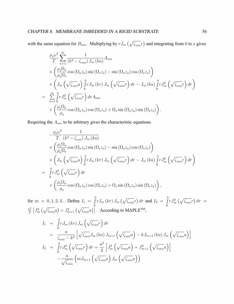
CHAPTER 8. MEMBRANE IMBEDDED IN A RIGID SUBSTRATE 56
with the same equation for Bmn. Multiplying by rJm�p�mnr
�and integrating from 0 to a gives
�s!2
T
1Xn=1
1
(k2 � �mn) Jm (ka)Amn
���sa�as
cos (aza) sin (szs)� sin (aza) cos (szs)�
��Jm
�p�mna
� aR0
rJm (kr) Jm
�p�mnr
�dr � Jm (ka)
aR0
rJ2m
�p�mnr
�dr
�=
1Pn=1
aR0
rJ2m
�p�mnr
�drAmn
���sa�a
cos (aza) cos (szs) + s sin (aza) sin (szs)
�:
Requiring the Amn to be arbitrary gives the characteristic equations
��s!2
T
1
(k2 � �mn) Jm (ka)
���sa�as
cos (aza) sin (szs)� sin (aza) cos (szs)�
��Jm
�p�mna
� aR0
rJm (kr) Jm
�p�mnr
�dr � Jm (ka)
aR0
rJ2m
�p�mnr
�dr
�=
aR0
rJ2m
�p�mnr
�dr
���sa�a
cos (aza) cos (szs) + s sin (aza) sin (szs)
�;
for m = 0; 1; 2; 3::: De�ne I1 =aR0
rJm (kr) Jm�p�mnr
�dr and I2 =
aR0
rJ2m�p�mnr
�dr =
a2
2
�J2m�p�mna
�+ J2m+1
�p�mna
��: According to MAPLETM,
I1 =aR0
rJm (kr) Jm
�p�mnr
�dr
=a
�mn � k2hp�mnJm (ka) Jm+1
�p�mna
�� kJm+1 (ka) Jm
�p�mna
�iI2 =
aR0
rJ2m
�p�mnr
�dr =
a2
2
hJ2m
�p�mna
�+ J2m+1
�p�mna
�i� ap
�mn
�mJm+1
�p�mna
�Jm
�p�mna
��

CHAPTER 8. MEMBRANE IMBEDDED IN A RIGID SUBSTRATE 57
which results in
��s!2
T
1
(k2 � �mn) Jm (ka)
���sa�as
cos (aza) sin (szs)� sin (aza) cos (szs)�
��Jm
�p�mna
�I1 � Jm (ka) I2
�� I2
���sa�a
cos (aza) cos (szs) + s sin (aza) sin (szs)
�= 0;m = 0; 1; 2; 3:::
Change of variables for analysis of the characteristic equation in MATLABTM requires that �mn =zapk2a � �mn, which implies that �mn = k2a �
��mnza
�2. This ensures the eigenvalues, �mn, will
be approximately evenly spaced, similar to the change of variables from the two-layer waveguide.The characteristic equation therefore becomes
��s!2
T
1
(k2 � �mn) Jm (ka)(8.9)
�
�s�mn
za�apk2s � �mn
cos (�mn) sin�zspk2s � �mn
�� sin (�mn) cos
�zspk2s � �mn
�!��Jm
�p�mna
�I1 � Jm (ka) I2
�+ I2
���s�mnza�a
cos (�mn) cos�zspk2s � �mn
�+pk2s � �mn sin (�mn) sin
�zspk2s � �mn
��= 0;m = 0; 1; 2; 3:::
8.1.2 Predicting ResonancesConsider equation (8.9). Substitution of s results in
��s!2
T
1
(k2 � �mn) Jm (ka)
���s�mnza�as
cos (�mn) sin (zss)� sin (�mn) cos (zss)�
��Jm
�p�mna
�I1 � Jm (ka) I2
�+ I2
���s�mnza�a
cos (�mn) cos (zss) +pk2s � �mn sin (�mn) sin (zss)
�= 0;m = 0; 1; 2; 3:::

CHAPTER 8. MEMBRANE IMBEDDED IN A RIGID SUBSTRATE 58
For a Z-resonance (� ! 0), assuming �a � �s,
��s!2
T
1
(k2 � k2a)sin�zspk2s � k2a
�(J0 (kaa) I1 � J0 (ka) I2)
+J0 (ka) I2
�cos�zspk2s � k2a
��= 0
withI1 =
a
k2a � k2(kaJ0 (ka) J1 (kaa)� kJ1 (ka) J0 (kaa))
andI2 =
a2
2
�J20 (kaa) + J
21 (kaa)
�� a
ka(mJ1 (kaa) J0 (kaa)) :
For an E-resonance (�mn ! 0);
��s!2
T(sin (zsks))
�J1 (ka)
k� J0 (ka)
a
2
�� ksk2J0 (ka)
a
2cos (zsks) = 0:
Recall that � = zapk2a � �mn, and � represents the resonant properties of the membrane. These
equations are plotted over a broad range of frequencies for the Sabatier parameters (�g (8.1)).
8.1.3 The Radial Continuity ConditionsThe �rst of the radial continuity conditions (8.6) gives
1Pm=0
1Pn=1
H(1)m
�p�na�(Cmn cos (m�) +Dmn sin (m�))Zn (z)
+1Pm=0
1Pn=1
� i
2"m�nH(1)m
�p�nr0
�Jm�p�na�cos (m (�0 � �))
�� (z0)Zn (z0)Zn (z)
=1Pm=1
1Pn=1
Jm
�p�mna
�(Amn cos (m�) +Bmn sin (m�))�mn (z)
where
�mn (z) =
�sin (a (z � za)) 0 � z � za
�sa�as
cos (aza) sin (sz)� sin (a (za)) cos (sz) zs � z < 0:
The second of the radial continuity conditions (8.6) gives1Pm=0
1Pn=1
p�nH
(1)0m
�p�na�(Cmn cos (m�) +Dmn sin (m�))Zn (z)
+1Pm=0
1Pn=1
�ip�n
2"m�nH(1)m
�p�nr0
�J 0m�p�na�cos (m (�0 � �))� (z0)Zn (z0)Zn (z)
=1Pm=1
1Pn=1
p�mnJ
0m
�p�mna
�(Amn cos (m�) +Bmn sin (m�))�mn (z) :

CHAPTER 8. MEMBRANE IMBEDDED IN A RIGID SUBSTRATE 59
Figure 8.1: Eigenvalues of the Membrane Problem. The eigenvalues corresponding to frequenciesare determined from the zero crossings.

CHAPTER 8. MEMBRANE IMBEDDED IN A RIGID SUBSTRATE 60
Equating the coef�cients of the trigonometric functions gives
1Pn=1
Jm
�p�mna
��mn (z)Amn �H(1)
m
�p�na�Zn (z)Cmn
= � i
2"m�nH(1)m
�p�nr0
�Jm�p�na�cos (m�0)� (z0)Zn (z0)Zn (z)
1Pn=1
Jm
�p�mna
��mn (z)Bmn �H(1)
m
�p�na�Zn (z)Dmn
= � i
2"m�nH(1)m
�p�nr0
�Jm�p�na�sin (m�0)� (z0)Zn (z0)Zn (z)
1Pn=1
p�mnJ
0m
�p�mna
��mn (z)Amn �
p�nH
(1)0m
�p�na�Zn (z)Cmn
= �ip�n
2"m�nH(1)m
�p�nr0
�J 0m�p�na�cos (m�0)� (z0)Zn (z0)Zn (z)
1Pn=1
p�mnJ
0m
�p�mna
��mn (z)Bmn �
p�nH
(1)0m
�p�na�Zn (z)Dmn
= �ip�n
2"m�nH(1)m
�p�nr0
�J 0m�p�na�sin (m�0)� (z0)Zn (z0)Zn (z) :
If �0 = 0 it suf�ces to consider the cosine equations. Multiplying by �Zn and integrating on z fromzs to za and using the orthogonality of the Zn gives
1Pl=1
Jm
�p� la�ImnlAml � �nH(1)
m
�p�na�Cmn
= ��ni
2"m�nH(1)m
�p�nr0
�Jm�p�na�� (z0)Zn (z0)
1Pl=1
p� lJ
0m
�p� la�ImnlAml � �n
p�nH
(1)0m
�p�na�Cmn
= ��nip�n
2"m�nH(1)m
�p�nr0
�J 0m�p�na�� (z0)Zn (z0)
where, according to MAPLETM,
�n =zaRzs
� (z)Zn (z)2 dz =
0Rzs
�aZs;n (z)2 dz +
zaR0
�sZa;n (z)2 dz
= ��azs2�
sin(�n)2(cos(�n) sin(�n) + �n) +
�sza2�n
cos(�n)2(� cos(�n) sin(�n) + �n)

CHAPTER 8. MEMBRANE IMBEDDED IN A RIGID SUBSTRATE 61
Imnl =zaRzs
� (z)�ml (z)Zn (z) dz =0Rzs
�a�ml;s (z)Zn;s (z) dz +zaR0
�s�ml;a (z)Zn;a (z) dz
=sin (�n) zs
za (��2mn + �2n)
��zs�s�mn cos (�mn) cos (�mn) + za�a�n sin (�n) sin (�mn)��mnza�a sin (�mn) sin (�mn) + zs�s�mn cos (�n) cos (�mn)
�+za�s cos (�n) (��mn cos (�mn) sin (�n) + �n sin (�mn) cos (�n))
�2n � � 2mnwhere
�n = zapk2a � �n
�n = zspk2s � �n
�mn = zapk2a � �mn
�mn = zspk2s � �mn
and
�n = k2a �
��nza
�2:
Eliminating Cmn gives1Pl=1
hp�nH
(1)0m
�p�na�Jm
�p� lma
��p� lmJ
0m
�p� lma
�H(1)m
�p�na�iImnlAml(8.10)
= �ip�n
2"m� (z0)Zn (z0)H
(1)m
�p�nr0
� " H(1)0m
�p�na�Jm�p�na�
�J 0m�p�na�H(1)m
�p�na� # :
Equation (8.10) is an in�nite dimensional linear system for Aml. In computing Aml, the in�nitelimit will be replaced by a suf�ciently high value, N , to form a �nite dimensional system. This isone of the equations that will be programmed into MATLABTM to solve the Membrane Problem.Note that C 0v (z) = �Cv+1 (z) + v
zCv (z), if C is a Bessel or Hankel Function.2 For simplicity,
rewrite equation (8.10), de�ning the �rst and second lines.
1Pl=1
hp�nH
(1)0m
�p�na�Jm
�p� lma
��p� lmJ
0m
�p� lma
�H(1)m
�p�na�iImnlAml (8.11)
= �ip�n
2"m� (z0)Zn (z0)H
(1)m
�p�nr0
� �H(1)0m
�p�na�Jm�p�na�� J 0m
�p�na�H(1)m
�p�na��:(8.12)
The bracketed portion of line (8.12) can be rewritten
H(1)0m
�p�na�Jm�p�na�� J 0m
�p�na�H(1)m
�p�na�
=
��H(1)
m+1
�p�na�+
mp�na
H(1)m
�p�na��Jm�p�na�
�H(1)m
�p�na���Jm+1
�p�na�+
mp�na
Jm�p�na��
2[2], pg. 361.

CHAPTER 8. MEMBRANE IMBEDDED IN A RIGID SUBSTRATE 62
Combining like terms yields
= Jm�p�na���H(1)
m+1
�p�na�+
mp�na
H(1)m
�p�na�� mp�na
H(1)m
�p�na��
+Jm+1�p�na�H(1)m
�p�na�
= Jm+1�p�na�H(1)m
�p�na�� Jm
�p�na�H(1)m+1
�p�na�
(8.13)
The bracketed portion of line (8.11) can be rewrittenp�nH
(1)0m
�p�na�Jm
�p� lma
��p� lmJ
0m
�p� lma
�H(1)m
�p�na�
=p�n
��H(1)
m+1
�p�na�+
mp�na
H(1)m
�p�na��Jm
�p� lma
��p� lmH
(1)m
�p�na� �Jm+1
�p� lma
�+
mp� lma
Jm
�p� lma
�!Combining like terms yields
= Jm
�p� lma
�� �p�nH
(1)m+1
�p�na�+p�n
mp�na
H(1)m
�p�na��p� lm
mp� lma
H(1)m
�p�na�!
+p� lmJm+1
�p� lma
�H(1)m
�p�na�
=p� lmJm+1
�p� lma
�H(1)m
�p�na��p�nJm
�p� lma
�H(1)m+1
�p�na�
(8.14)
Lines (8.13) and (8.14) were entered into the formula for Amn: Therefore,1Pl=1
hp� lmJm+1
�p� lma
�H(1)m
�p�na��p�nJm
�p� lma
�H(1)m+1
�p�na�iImnlAml
= �ip�n
2"m� (z0)Zn (z0)H
(1)m
�p�nr0
� " Jm+1�p�na�H(1)m
�p�na�
�Jm�p�na�H(1)m+1
�p�na� # :
The Cmn are then given by
Cmn =
1Pl=1
Jm�p� la�ImnlAml
�nH(1)m
�p�na� �
iH(1)m
�p�nr0
�Jm�p�na�� (z0)Zn (z0)
2"m�nH(1)m
�p�na� :
Velocity in the atmosphere is
w =1
i!�a@zp (8.15)
=1
i!�a
1Pm=0
1Pn=1
Jm
�p�mnr
�Amn cos (m�)�
0mn (z) ; r < a
CHAPTER 8. MEMBRANE IMBEDDED IN A RIGID SUBSTRATE 63
where�mn (z) = sin (a (z � za)) :
and�0mn (z) = a cos (a (z � za)) :

Chapter 9
Membrane Analysis and Comparison withSabatier1
9.1 Membrane AnalysisIn this section, the blue line in each graph represents the Sabatier parameters. All other colorsare variations on the indicated parameter. Note that the Sabatier parameters are zs = �0:175 m,ca = 340 m/s, �a = 1:2
kgm3 , ccomp;s = 160 m/s, cshear;s = 75 m/s, and �s = 1400
kgm3 :
9.1.1 Termination of the In�nite SumIn order to obtain reasonable solutions, it is necessary to extend the solution in equation (8.15) toat least the �rst soil eigenvalue. This eigenvalue results from equation (4.18), particularly fromthe cos zs
pk2s � � in the �rst line. Since cos (x) = 0 when x =
(2n�1)�2
, zspk2s � � =
(2n�1)�2
:
Therefore, � = k2s ��(2n�1)�2zs
�2! � = za
rk2a � k2s +
�(2n�1)�2zs
�2: Since the �rst soil resonance
is of interest, n = 1; and � = za
rk2a � k2s +
��2zs
�2: With the appropriate substitutions made,
� = 500
s�2�fca
�2��2�f
�2�f+i �
�p
�c2ss
�+��2zs
�2. To ensure that the �rst resonance is completely
accounted for, � + 1000 will be used to terminate the in�nite sum. Figure (9.1) represents earlyand late termination of the sum, around this predicted value, for the �rst mechanical resonance forthe Sabatier parameters.
64

CHAPTER 9. MEMBRANE ANALYSIS AND COMPARISON WITH SABATIER2 65
Figure 9.1: This �gure represents the effects of early termination of the in�nite sum. Note theexaggeration and unreasonable difference in magnitude between the resonance. The vertical scaleis 1� 10�3:

CHAPTER 9. MEMBRANE ANALYSIS AND COMPARISON WITH SABATIER3 66
Figure 9.2: This graphic shows how increasing the depth results in much weaker mechanical andacoustic resonances. Note how the resonances change with depth. The vertical scale is 1� 10�6:The units of zs are meters.

CHAPTER 9. MEMBRANE ANALYSIS AND COMPARISON WITH SABATIER4 67
Figure 9.3: Results of varying the compressional wave speed within the Sabatier parameters. Theunits of cp;s are m/s.
9.1.2 Variance of ParametersDepth of Mine Detection Limitations
As seen in Figure (9.2), as depth increases, the mechanical resonance moves to the right anddecreases in strength. If the large mechanical resonance disappears, the acoustical resonance isalso very hard to detect. The resonance of the mine itself is much stronger than the acousticresonance. Resonances at larger depths are soil resonances, and can be predicted from the two-layer waveguide. According to Sabatier, landmines are usually buried less than 10 centimeters (.1m) from the soil surface. As indicated by Figure (9.2), the soil particle velocity plots are moreprecise at shallow depths.
Soil Variations
Compressional sound speed (�g. (9.3)) affects the curvature, location, and magnitude of the reso-nance. Larger values for compressional sound speed move the resonances to the left, and decreasethe curvature of the leading part of the resonance. There does not appear to be any correlation
1[27]

CHAPTER 9. MEMBRANE ANALYSIS AND COMPARISON WITH SABATIER5 68
Figure 9.4: Results of varying the shear wave speed within the Sabatier parameters. The units ofcs are m/s. The vertical scale is 1� 10�5:
between large and small values with magnitude; however, magnitude does show some dependenceon compressional wave speed. Note that Sabatier suggests a value of 160 m
s, while experiments
from Dr. D. Keith Wilson and Dr. Harley Cudney of the US Army Corps of Engineers suggestvalues may be as high as 647m
sin shallow desert soil. With such a large variance in soil parame-
ters, ascertaining the effect of sound speed on the pro�les is a very important step in predicting thelandmine resonances.According to Figure (9.4), larger values of shear sound speed appear to move the resonance to
the right, and decrease the intensity of the soil velocity response.Similarly, the density of the soil appears to have signi�cant effect (�g. (9.5)). This parameter
seems to adjust resonance width, amplitude, and a slight shift in the resonant frequency. The onlyapparent correlation is between the magnitude of �p and the resonance shift: small �p appear tothe right of larger values for �p: Sabatier suggests a value of 1400
kgm3 , while the experimental data
from Wilson and Cudney suggest 1600 kgm3 . Note that �s = �p + i�
!; and that the �p was altered
by changing �s; the value given the key for the graph.

CHAPTER 9. MEMBRANE ANALYSIS AND COMPARISON WITH SABATIER6 69
Figure 9.5: This graphic demonstrates the sensitivity of the soil particle velocity to changes in�p:The vertical scale is 1� 10�6:

CHAPTER 9. MEMBRANE ANALYSIS AND COMPARISON WITH SABATIER10 70
Figure 9.6: This pro�le shows the effect of the size of the mine with regard to the resonance. Noteeven small changes in the radius a seem to have large effects. The vertical scale is 1� 10�5:
9.1.3 Membrane VariationThe membrane density and tension are dif�cult quantities to assign since they are particular toeach landmine. Since this model is based on the VS 1.6 Anti-Tank mine, a brief discussion ofthe selection process for �m follows in the discussion on the comparison with Sabatier's model.However, this discussion suggests that either the mechanical resonance or exact parameters withregard to both tension and density must be known for accurate detection.The size of the landmine also affects detectability. The VS 1.6 is approximately the size of a
dinner plate, with a radius of 7 centimeters (.07 m). However, the smaller the mine, the smallerthe amplitude of the resonances, making the mine harder to detect. This is shown in Figure (9.6).Note that small changes (not even order of magnitude changes) have a large effect on the resonantfrequencies.
CHAPTER 9. MEMBRANE ANALYSIS AND COMPARISON WITH SABATIER13 71
9.2 Comparison with Sabatier's Findings
9.2.1 The Sabatier - Waxler - Velea Paper7
In An Effective Fluid Model for Landmine Detection using Acoustic to Seismic Coupling, Sabatieret. al create a "right circular waveguide with rigid walls, [which] contains air in the upper half,soil in the lower half, and a buried mine placed concentrically on the waveguide's axis."8 Usinga mass-spring problem analogy, Sabatier then uses a "brute force numerical scheme"9 to solve thepressure equation, using the same boundary conditions as this project. The paper from Sabatier etal. does not consider the scattering effects of the mine or soil for an incident acoustic or seismicwave; whereas this project has included the scattering effects.The Sabatier parameters refer to the properties used by Sabatier in his research. The �rst
parameter described is the depth of the buried mine, referred to as zs in this project, at 3 inches, or0.075 meters. The mine's radius is next mentioned, referred to as a in this project, and assigneda value of 0.07 meters. The frequency sweep that Sabatier performs ranges from f = 80 � 300Hz. Finally, the air and soil parameters that Sabatier uses are listed as ca = 340 m/s, �a = 1:2
kgm3 ,
cs = 160 m/s, and �s = 1400kgm3 :
9.2.2 Selection of �m, the Density of the MembraneThe selection of �m, along with other variables, determines the resonances for the soil-membranesystem. Sabatier's model of the system as a mass-spring damper lists parameters speci�c to themass and spring that cannot be easily translated into values for this project. Expecting that themechanical resonance should occur at approximately 100 Hz, reasonable approximations are madefrom the mathematical equations for �m: From equation (8.9), a mechanical resonance occurswhen J0 (ka) = 0, where k 2 R: Recall that k =
q�m!
2+i�m!T
is actually complex, where ! isthe angular frequency (! = 2�f ), �m accounts for the damping, and T is the tension. The �rstzero of the Bessel function occurs when ka = 2:405:11 If a = :07 m, as in Sabatier's experiment,then k = 34:3571 �
q�m!
2
T: Sabatier's parameters are assumed for the other variables to be
! = 2� (100) Hz; �m = 1000 N-s/m; and T = 2; 000; 000 kg/s2, then �m = 5980:04 � 6000kg/m3:
9.2.3 Comparison with Sabatier's WorkA mechanical resonance is de�ned as "the resonant frequencies of any mechanical system forwhich the input mechanical reactance goes to zero."12 The mechanical system refers to the land-mine itself, explaining the narrow band response observed in this paper's frequency response graph.
7[27]8[27], pg. 1993.9[27], pg. 1996.11[5], pg. x.12[18], pg. 48.

CHAPTER 9. MEMBRANE ANALYSIS AND COMPARISON WITH SABATIER14 72
Figure 9.7: Sabatier's measured values in a soil surface velocity plot. Note the increments areapproximately 10 Hz.

CHAPTER 9. MEMBRANE ANALYSIS AND COMPARISON WITH SABATIER15 73
Figure 9.8: Predictions based on the theoretical solution presented in this paper for Sabatier'sparameters.

CHAPTER 9. MEMBRANE ANALYSIS AND COMPARISON WITH SABATIER17 74
Man-made objects, like a landmine case, tend to have a relatively narrow band response due to thehighly organized molecular structure of the solid material when compared with the granular andsigni�cantly more random structure of the soil particles. This higher quality factor "Q" responseallows acoustic to seismic landmine detection to remain fairly accurate (in discriminating detec-tions from false alarms) in even rocky soil, where conventional detection techniques fail. Note thecommon resonance in the Sabatier plot (�g. (9.7)) and this project's plot (�g. (9.8)) at approxi-mately 100 Hz.The anti-resonance is the frequencies which result in a local minimum for the frequency re-
sponse plot. This can be compared to the destructive interference between two propagating waves.Sabatier claims the anti-resonance occurs from 180-210 Hz, while the data from this paper suggestsanti-resonances occur precisely before the mechanical resonances.The prediction also suggests a second mechanical resonances for the membrane at approxi-
mately 230 Hz.There appears to be a peak in Sabatier's work near f = 240 Hz that is unlabeled. This is a soil
resonance, predicted by the two-layer waveguide problem in this paper (see �g. (9.9)). The samesoil resonance is observed in the plot from this project's derivation.The �rst acoustical resonance is term de�ned by Sabatier to be the frequency at which "the layer
of soil between the top of the mine and the surface of the soil"16 vibrates at maximum amplitude.This resonance occurs very clearly in Sabatier's graph at approximately f = 280 Hz. However,according to Figure (9.9), the second soil resonance occurs at this same frequency.
16[27], pg. 1994.

CHAPTER 9. MEMBRANE ANALYSIS AND COMPARISON WITH SABATIER18 75
Figure 9.9: This plot shows the predicted soil resonances for the false alarm case, generated fromthe two-layer waveguide using the Sabatier parameters.
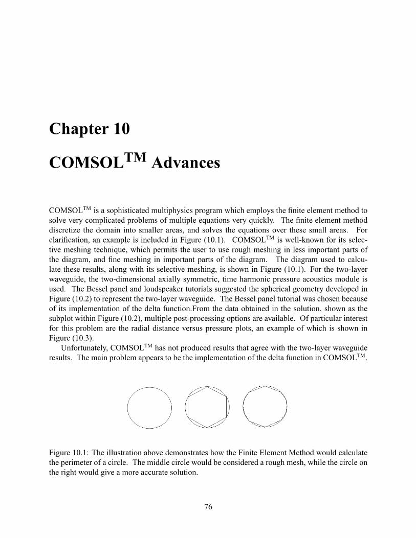
Chapter 10
COMSOLTM Advances
COMSOLTM is a sophisticated multiphysics program which employs the �nite element method tosolve very complicated problems of multiple equations very quickly. The �nite element methoddiscretize the domain into smaller areas, and solves the equations over these small areas. Forclari�cation, an example is included in Figure (10.1). COMSOLTM is well-known for its selec-tive meshing technique, which permits the user to use rough meshing in less important parts ofthe diagram, and �ne meshing in important parts of the diagram. The diagram used to calcu-late these results, along with its selective meshing, is shown in Figure (10.1). For the two-layerwaveguide, the two-dimensional axially symmetric, time harmonic pressure acoustics module isused. The Bessel panel and loudspeaker tutorials suggested the spherical geometry developed inFigure (10.2) to represent the two-layer waveguide. The Bessel panel tutorial was chosen becauseof its implementation of the delta function.From the data obtained in the solution, shown as thesubplot within Figure (10.2), multiple post-processing options are available. Of particular interestfor this problem are the radial distance versus pressure plots, an example of which is shown inFigure (10.3).Unfortunately, COMSOLTM has not produced results that agree with the two-layer waveguide
results. The main problem appears to be the implementation of the delta function in COMSOLTM.
Figure 10.1: The illustration above demonstrates how the Finite Element Method would calculatethe perimeter of a circle. The middle circle would be considered a rough mesh, while the circle onthe right would give a more accurate solution.
76

CHAPTER 10. COMSOLTM ADVANCES 77
Figure 10.2: This diagram shows the geometry of the COMSOL model drafted for the two-layerwaveguide. A quarter circle with a radius of 500 representing the atmospheric layer was placedatop a rectangle of depth 1 meter. Appropriate boundary conditions were selected, and the solutionin the location around the point source is shown as an insert.
The source in the problem plotted in Figure (10.3) was at r0 = 0, so the highest pressure shouldlogically appear at r � 0. The COMSOLTM solution is still being worked on, and hopefully aresult matching the MATLABTM computed two-layer waveguide will be obtained.

CHAPTER 10. COMSOLTM ADVANCES 78
Figure 10.3: An example of a radial distance versus pressure plot for the two-layer waveguide.

Bibliography
[1] Interview with SPC Daniel P. Staciak, USA, 2d Battalion, 87th Inf, 3rd Brigade, 10thMountian Division. Deployment from 05 February, 2006 - 25 May, Afganistan, 2007.
[2] M. Abramowitz and I. Stegun, editors. Handbook of Mathematical Functions. Dover, NewYork, 1965.
[3] K. Attenborough, S. Taherzadeh, H. Bass, R. Raspet, G. Becker, A. Gudesen, A. Chrestman,G. Daigle, A. L'Esperance, Y. Gabillet, K. Gilbert, Y. Li, M. White, P. Naz, J. Noble, andH. van Hoof. Benchmark cases for outdoor sound propagation models. J. Acoust. Soc. Am.,97(1):173�191, 1995.
[4] P. Bergmann. The wave equation in a medium with a variable index of refraction. J. Acoust.Soc. Am., 17:329�333, 1946.
[5] F. Bowman. Introduction to Bessel Functions. Dover Publications Inc., New York, 1958.
[6] C. Boyles. Acoustic Waveguides. John Wiley and Sons, New York, 1984.
[7] M. Croll. The History of Landmines. Pen and Sword Books, Ltd., Barnsley, Great Britian,1998.
[8] M. O. R. Darmody and W. O'Brien. Measurement of attenuation and speed of sound in soils.Soil Sci. Soc. Am. J., 66:788�796, 2002.
[9] G. Frisk. Ocean and Seabed Acoustics. Prentice Hall, Englewood Cliffs, New Jersey, 1994.
[10] E. Gossard. Waves in the Atmosphere. Elsevier, Amsterdam, 1975.
[11] R. Haberman. Applied Partial Differential Equations. Pearson Education, Inc., Boston, 2004.
[12] R. Hackman. Acoustical scattering in an inhomogeneous waveguide:theory. J. Acoust. Soc.Am., 80:1447�1458, 1986.
[13] N. Haskell. Asymptotic approximation for the normal modes in sound channel wave propa-gation. J. Appl. Phys., 22:157�168, 1951.
[14] A. Healey and W. Webber. Sensors for the detection of land-based munitions. DefenseTechnical Information Center - Naval Postgraduate School, Monterey, California, 1995.
79

BIBLIOGRAPHY 80
[15] C. Hines. Atmospheric gravity waves: A new toy for the wave theorist. Radio Sci., 69:375�380, 1965.
[16] F. Ingenito. Scattering from an object in a strati�ed medium. J. Acoust. Soc. Am., 82:2051�2059, 1987.
[17] A. Kharab and R. Guenther. An Introduction to Numerical Methods. Chapman and Hall,London, 2006.
[18] A. C. L.E. Kinsler, A.R. Frey and J. Sanders. Fundamentals of Acoustics, 4th Edition. JohnWiley and Sons, New York, 2000.
[19] J. MacDonald, J. Lockwood, J. McFee, T. Altshuler, T. Broach, L. Carin, R. Harmon, C. Rap-paport, W. Scott, and R. Weaver. Alternatives for Landmine Detection. RAND Science andTechnology Policy Institute, Santa Monica, California, 2003.
[20] J. Mathews and R. Walker, editors. Mathematical Methods of Physics. Addison Wesley,Boston, 1971.
[21] R. McGrath. Landmines and Unexploded Ordnance: A Resource Book. Pluto Press, London,2000.
[22] P. Morse and K. Ingard. Theoretical Acoustics. Princeton University Press, Princeton, NewJersy, 1968.
[23] F. I. N. Makris and W. Kuperman. Detection of a submerged object insoni�ed by surfacenoise in an ocean waveguide. J. Acoust. Soc. Am., 96(3):1703�1724, 1994.
[24] E. Sengpiel. für Mikrofonaufnahmetechnik und Tonstudiotechnik - Microphone for RecordingTechnique and Recording Studio Technology. online at sengpielaudio.com, University of theArts, Berlin.
[25] A. Sommerfeld, editor. Partial Differential Equations of Physics. Academic Press, NewYork, 1964.
[26] E. Toolbox. Density of Dry Air, Water Vapor, and Moist Humid Air. online at engineering-toolbox.com, The Engineering Toolbox.
[27] D. Velea, R. Waxler, and J. Sabatier. An effective �uid model for landmine detection usingacoustic to seismic coupling. J. Acoust. Soc. Am., 115(5):1993�2002, 2004.
[28] N. Youngblood. The Development of Mine Warfare. Praeger Security International, Westport,Conneticut, 2006.
[29] C. Zwikker and C. Kosten. Sound Absorbing Materials. Elsevier Publishing Corp., NewYork, 1949.

Appendix A
Orthogonality Proofs
A.1 Orthogonality of the EigenfunctionsThe generic Sturm-Liouville Differential Equation in the z coordinate is represented by
@
@z
�p (z)
@Z
@z
�+ [�� (z) + q (z)]Z = 0: (A.1)
In the case of the two layer waveguide problem,
Z 00a (z) +���+ k2a
�Za (z) = 0
Z 00s (z) +���+ k2s
�Zs (z) = 0
p (z) = 1, � = ��, and q (z) =�k2a 0 < z � zak2s za � z < 0
, to obtain the Z (z) =�Za 0 < z � zaZs zs � z < 0
function. Let Zm and Zn be eigenfunctions of the depth equation (Z (z)). The following proofimplies that eigenfunctions Zm and Zn of the Sturm-Liouville equation are orthogonal on (a; b)with respect to the weight function � (z) if
bRa
Zm (z) (p (z)Z0n (z))
0dz +
bRa
q (z)Zm (z)Zn (z) dz + �nbRa
� (z)Zm (z)Zn (z) dz = 0: (A.2)
In the case of the two layer waveguide problem, the condition above refers to the two intervals of(zs; 0) and (0; za), written as
0Rzs
Zs;m (z)Z00s;n (z) dz +
0Rzs
k2sZs;m (z)Zs;n (z) dz � �n0Rzs
� (z)Zs;m (z)Zs;n (z) dz = 0
zaR0
Za;m (z)Z00a;n (z) dz +
zaR0
k2aZa;m (z)Za;n (z) dz � �nzaR0
� (z)Za;m (z)Za;n (z) dz = 0:
81

APPENDIX A. ORTHOGONALITY PROOFS 82
Using integration by parts on the �rst integral of both conditions gives
bRa
Zm (z) (p (z)Z0n (z))
0dz = Zm (z) p (z)Z
0n (z) jba �
bRa
p (z)Z 0m (z)Z0n (z) dz
or, in the speci�c cases presented in this paper,
0Rzs
Zs;m (z)Z00s;n (z) dz = Zs;m (z)Z
0s;n (z) j0zs �
0Rzs
Z 0s;m (z)Z0s;n (z) dz
zaR0
Za;m (z)Z00a;n (z) dz = Za;m (z)Z
0a;n (z) jza0 �
zaR0
Z 0a;m (z)Z0a;n (z) dz:
The governing boundary conditions are that Z (za) = 0, Za (0) = Zs (0), �sZ 0a (0) = �aZ 0s (0) andZ 0 (zs) = 0. Therefore,
Zs;m (z)Z0s;n (z) j0zs = Zs;m (0)Z
0s;n (0)� Zs;m (zs)Z 0s;n (zs) = Zs;m (0)Z 0s;n (0)
Za;m (z)Z0a;n (z) jza0 = Za;m (za)Z
0a;n (za)� Za;m (0)Z 0a;n (0) = �Za;m (0)Z 0a;n (0)
= ��a�sZs;m (0)Z
0s;n (0) :
So,
Zs;m (0)Z0s;n (0)�
0Rzs
Z 0s;m (z)Z0s;n (z) dz+
0Rzs
k2sZs;m (z)Zs;n (z) dz��n0Rzs
� (z)Zs;m (z)Zs;n (z) dz = 0
0 = �Za;m (0)Z 0a;n (0)�zaR0
Z 0a;m (z)Z0a;n (z) dz
+zaR0
k2aZa;m (z)Za;n (z) dz � �nzaR0
� (z)Za;m (z)Za;n (z) dz:
Switchingm and n gives
0 = Zs;n (0)Z0s;m (0)�
0Rzs
Z 0s;n (z)Z0s;m (z) dz
+0Rzs
k2sZs;n (z)Zs;m (z) dz � �m0Rzs
� (z)Zs;n (z)Zs;m (z) dz
0 = �Za;n (0)Z 0a;m (0)�zaR0
Z 0a;n (z)Z0a;m (z) dz
+zaR0
k2aZa;n (z)Za;m (z) dz � �mzaR0
� (z)Za;n (z)Za;m (z) dz:

APPENDIX A. ORTHOGONALITY PROOFS 83
Subtracting the two equations, respectively, results in
Zs;m (0)Z0s;n (0)� Zs;n (0)Z 0s;m (0)� (�n � �m)
0Rzs
� (z)Zs;n (z)Zs;m (z) dz = 0
�Za;m (0)Z 0a;n (0) + Za;n (0)Z 0a;m (0)� (�n � �m)zaR0
� (z)Za;n (z)Za;m (z) dz = 0:
Note that the second equation above is actually
��a�s
�Zs;m (0)Z
0s;n (0)� Zs;n (0)Z 0s;m (0)
�� (�n � �m)
zaR0
� (z)Za;n (z)Za;m (z) dz = 0
or
�Zs;m (0)Z 0s;n (0) + Zs;n (0)Z 0s;m (0)��s�a(�n � �m)
zaR0
� (z)Za;n (z)Za;m (z) dz = 0
so that the �rst equation added to the equivalent second equation is
� (�n � �m)0Rzs
� (z)Zs;n (z)Zs;m (z) dz ��s�a(�n � �m)
zaR0
� (z)Za;n (z)Za;m (z) dz = 0
��a (�n � �m)0Rzs
� (z)Zs;n (z)Zs;m (z) dz � �s (�n � �m)zaR0
� (z)Za;n (z)Za;m (z) dz = 0
� (�n � �m)"�a
0Rzs
� (z)Zs;n (z)Zs;m (z) dz + �szaR0
� (z)Za;n (z)Za;m (z) dz
#= 0:
Assuming �n 6= �m when n 6= m,zaRzs
� (z)Zn (z)Zm (z) = 0
whereZn (z)Zm (z) =
�Za;n (z)Za;m (z) dz when 0 < z � zaZs;n (z)Zs;m (z) dz when zs � z < 0
implies Z is orthogonal with respect to the weight function
� (z) =
��s when 0 < z � za�a when zs � z < 0
:

Appendix B
Additional Proofs
B.1 Explanation of the Exclusion of Gravity from the Conser-vation of Momentum Equation
The exclusion of the gravity term from the derivation of momentum originates from the following
Although gravity is always present, it has negligible in�uence on acoustic distur-bances of all but extremely low frequencies, e.g., those of order or less than g
c, where
g is the acceleration due to gravity and c is the speed of sound; so, for simplicity, thebody force term is neglected at the outset. Acoustic-gravity waves [internal waves](infrasonic waves with frequencies so low as to be strongly affected by gravity) havebeen a major topic of research during the past two decades but fall outside the scopeof an introductory discussion.1
Since cs = 160 m= s, and g = 9:8m= s2, gc =160m= s9:8m= s2
= 16: 327Hz � 100Hz, which is thelowest frequency of interest.
B.2 Proof of the Denominator in equation (4.25) Using Hand-book of Mathematical Functions2
The denominator �rst reads
�p�lH(1)0k
�p�lr0
�Jk�p�lr0
�+p�lH
(1)k
�p�lr0
�J 0k�p�lr0
�By Abramowitz and Stegun,3 the derivative of a Bessel or Hankel function can be simpli�ed into
1[4],[13],[15],[10]2[2], pg. 362.3[2], pg. 362, eqn. (9.1.27).
84

APPENDIX B. ADDITIONAL PROOFS 85
�p�l
��p�lr0
�H(1)k+1
�p�lr0
�+ kH
(1)k
�p�lr0
�p�lr0
!Jk�p�lr0
�+p�lH
(1)k
�p�lr0
� � �p�lr0� Jk+1 �p�lr0�+ kJk �p�lr0�p�lr0
!
Simplifying the denominator of the equation yields�p�lr0
� hH(1)k+1
�p�lr0
�Jk�p�lr0
��H(1)
k
�p�lr0
�Jk+1
�p�lr0
�ir0
+khH(1)k
�p�lr0
�Jk�p�lr0
��H(1)
k
�p�lr0
�Jk�p�lr0
�ir0
Recognizing that the second part of the equation is zero gives�p�l� hH(1)k+1
�p�lr0
�Jk�p�lr0
��H(1)
k
�p�lr0
�Jk+1
�p�lr0
�i+ 0
Multiplying to use Abramowitz and Stegun,4
p�l2
"H(1)k+1
�p�lr0
�H(1)k
�p�lr0
�+H
(1)k+1
�p�lr0
�H(2)k
�p�lr0
��H(1)
k
�p�lr0
�H(1)k+1
�p�lr0
��H(1)
k
�p�lr0
�H(2)k+1
�p�lr0
� #
Applying Abramowitz and Stegun5 givesp�l2
hH(1)k+1
�p�lr0
�H(2)k
�p�lr0
��H(1)
k
�p�lr0
�H(2)k+1
�p�lr0
�i=
p�l2
�� 4i
�p�lr0
�= � 2i
�r0
4[2], pg. 362, eqn. (9.1.17).5[2], pg. 362, eqn. (9.1.17).

Appendix C
Graph Parameters
C.1 Common ValuesNote that units have been dropped for the numerical analysisza = 500ca = 330�a = 1:168� = 0rtol = 5� 10�5�m = 1000T = 2� 106a = 0:07m = 0
C.2 Values for Speci�c FiguresFigures (4.2) and (8.1):zs = �0:075cs = 170cp = 75r0 = 2z0 = 2�0 = 0r = 0:0z = 0� = 0Figures (4.3), (4.4), (6.1), (6.2), (6.3), (6.5), (6.6), (6.7), and (6.4):zs = �1cs = 160
86

APPENDIX C. GRAPH PARAMETERS 87
r0 = 2z0 = 2�0 = 0r = 0:0z = 0� = 0Figures (9.1), (9.2), (9.3), (9.4), (9.5), (9.6), and (9.8):zs = �0:175cs = 170cp = 75r0 = 0:2z0 = 2�0 = 0r = 0:0z = 0� = 0

Appendix D
MATLABTM Files
D.1 Common Functions
D.1.1 csqrt.mfunction y=csqrt(z)y=sqrt(z);iset=�nd(imag(z)<0);y(iset)=-y(iset);
D.1.2 eigs4z.mfunction Z=eigs4z(kap,rhoa,rhos,za,ca,zs,cs,sigma,rhop,f)omega=2*pi*f;ks=sqrt((omega^2+i*omega*sigma/rhop)/cs^2);ka=omega/ca;%ps=-i*omega*rhop/(sigma+i*omega*rhop);llamb = sqrt(ks^2-ka^2+kap.^2/za^2);Z=rhos*(cos(kap).*cos(zs*llamb)).*(kap/za)+rhoa*(sin(kap).*sin(zs*llamb)).*llamb;
D.1.3 mu.mfunction [mu,kappa]=mu(n,ka,rhoa,rhos,za,ca,zs,cs,sigma,rhop,f)ftntol=5e-4;sectol=5e-4;count=1;for ii=n[kap,fv] = secant(@(kap1) eigs4z(kap1,rhoa,rhos,za,ca,zs,cs,sigma,rhop,f),(2*ii-1)*pi/2-pi/8,(2*ii-1)*pi/2+pi/8,sectol);if (fv<ftntol)&(real(kap)>(ii-1)*pi)&(real(kap)<ii*pi)
88

APPENDIX D. MATLABTM FILES 89
kappa(count)=kap;elsek1=(2*ii-1)*pi/2-1.57;k2=(2*ii-1)*pi/2+1.57;kapr=linspace(k1,k2,100);y=real(eigs4z(kapr,rhoa,rhos,za,ca,zs,cs,sigma,rhop,f));if y(1)>0I=�nd(y<0);elseI=�nd(y>0);endif isempty(I)if count == 1kappa(count) = 0;elseFigureplot(kapr,y)error('zero not found')endelse[kap,fv]=secant(@(kap1) eigs4z(kap1,rhoa,rhos,za,ca,zs,cs,sigma,rhop,f),kapr(I(1))-.1,kapr(I(1))+.1,sectol);kappa(count)=kap;endendcount=count+1;endif abs(kappa(1))<sectolkappa=kappa(2:end);endmu=ka^2-(kappa/za).^2;
D.1.4 rho.mfunction wrho=rho(z,rhos,rhoa)if z>=0wrho=rhos;elsewrho=rhoa;end

APPENDIX D. MATLABTM FILES 90
D.2 Two-Layer Waveguide Speci�c Programs
D.2.1 dZn.mfunction dZ=dZn(z,ka,muv,za,ks,zs)if z>=0dZ=(ka^2-muv).^(1/2).*sin((ka^2-muv).^(1/2)*za)./cos((ka^2-muv).^(1/2)*za).*sin((ka^2-muv).^(1/2)*z)+(ka^2-muv).^(1/2).*cos((ka^2-muv).^(1/2)*z);elsedZ=sin((ks^2-muv).^(1/2)*zs)./cos((ks^2-muv).^(1/2)*zs).*sin((ka^2-muv).^(1/2)*za)./cos((ka^2-muv).^(1/2)*za).*((ks^2-muv).^(1/2).*cos((ks^2-muv).^(1/2)*zs)./sin((ks^2-muv).^(1/2)*zs).*sin((ks^2-muv).^(1/2)*z)+(ks^2-muv).^(1/2).*cos((ks^2-muv).^(1/2)*z));end
D.2.2 eigsplot.mza=500; %rough estimate of the upper limit of the problem, units of mca=330; % speed of sound, m/szs=-1; %rough estimate of lower limit of problem, units of mcs=160; %Attenborough et al. Attached derivation from Buchanan units m/ssigma = 0; %366000;rhop = 4150;rhoa=1.168; %Wikipedia, density of dry air at std ambient press and temp%Density of Air Article, units of kg/m^3r0=2;z0=2;theta0=0;NBlock = 250;r=1;theta=0;p=[];rtol = 5e-5;f=50;omega=2*pi*f;rhos=rhop+i*sigma/omega;kappa=linspace(0,20,100);Y=eigs4z(kappa,rhoa,rhos,za,ca,zs,cs,sigma,rhop,f);plot(kappa,Y,'b')

APPENDIX D. MATLABTM FILES 91
D.2.3 gui.mdisp('Predicted Soil Resonances for Landmine Detection')disp('*******************************************************************')disp('Effective Fluid Model developed by Mattingly and Buchanan')disp(' ')disp('This method for determining soil resonances uses linearized Partial')disp('Differential Equations to approximate the behavior at the air-soil')disp('interface.')disp(' ')disp('*******************************************************************')disp(' ')disp('All input values are in the assigned units')disp(' ')za=500;rsp=input('For advanced selections, press any numeric key now');if isempty(rsp)typ2=input('Enter the ambient temperature (C)');if typ2<=-10rhoa1=1.341;ca1=325.4;elseif (typ2>-10)&(typ2<=-5)rhoa1=1.316;ca1=328.5;elseif (typ2>-5)&(typ2<=0)rhoa1=1.293;ca1=331.5;elseif (typ2>0)&(typ2<=5)rhoa1=1.269;ca1=334.5;elseif (typ2>5)&(typ2<=10)rhoa1=1.247;ca1=337.5;elseif (typ2>10)&(typ2<=15)rhoa1=1.225;ca1=340.5;elseif (typ2>15)&(typ2<=20)rhoa1=1.204;ca1=343.4;elseif (typ2>20)&(typ2<=25)rhoa1=1.184;ca1=346.3;elseif (typ2>25)&(typ2<35)

APPENDIX D. MATLABTM FILES 92
ca1=349.2;rhoa1=1.164;elserhoa1=1.1;ca1=331.4+.6*typ2;endtyp3=input('Enter the humidity in decimal form');rhoa=rhoa1*(1+typ3)/(1+1.609*typ3);ca=ca1+typ3*.6*ca1;typ1=input('Select soil type: 1=sand, 2=silt, 3=clay, 4=organic matter');typ11=input('Select soil moisture (scale of 1-5, 1=dry, 5=saturated)');typ12=input('Select soil compaction (scale of 1-4, 1=loose, 4=dense)');if typ1 == 1if typ11 == 1cs=260;elseif typ11 == 2if typ12 <3cs = 138;elsecs = 103;endelseif typ11==3if typ12 < 3cs=122;elsecs=253;endelsecs=189;endelseif typ1 == 2if typ11 == 1if typ12 <3cs=140;elsecs=139;endelseif typ11 == 2if typ12 <3cs = 117;elsecs = 122;

APPENDIX D. MATLABTM FILES 93
endelseif typ11==3if typ12 < 3cs=121;elsecs=176;endelsecs=207;endelseif typ1 == 3if typ11 == 1if typ12 <3cs=177;elsecs=159;endelseif typ11 == 2if typ12 <3cs = 118;elsecs = 136;endelseif typ11==3if typ12 < 3cs=107;elsecs=245;endelsecs=118;endelseif typ1 == 4if typ11 == 1if typ12 <3cs=153;elsecs=121;endelseif typ11 == 2if typ12 <3cs = 89;

APPENDIX D. MATLABTM FILES 94
elsecs = 147;endelseif typ11==3if typ12 < 3cs=87;elsecs=86;endelsecs=102;endelsedisp('Error in submission of soil type')endcp=270;sigma=0;endrtol = 5e-4;NBlock = 250;if ~isempty(rsp)ca=input('Enter the speed of sound in the atmosphere (m/s)');if isempty(ca)ca=343;endcp=input('Enter the speed of shear sound waves in the soil (m/s)');if isempty(cs)cs=210.31;endcs=input('Enter the speed of compressional sound waves in the soil (m/s)');if isempty(cp)cp=647;endsigma=input('Enter the �ow resistivity in the soil (Pa*s/m^2)');if isempty(sigma)sigma=0;endrhoa=input('Enter the density of the atmosphere (kg/m^3)');if isempty(rhoa)rhoa=1.205;endrtol=input('Enter the tolerance');

APPENDIX D. MATLABTM FILES 95
if isempty(rtol)rtol=5e-5;endendNBlock=250;zs=input('Enter the depth of the soil (m)');if isempty (zs)zs=-1;endAA=input('Enter the position of the source[radial component, azmuthal component, height component] (m)');r0=AA(1);theta0=AA(2);z0=AA(3);r=0;theta=0;z=0;CC=input('Enter the frequency range of interest[lowest frequency,highest frequency] (Hz)');p=[];rhop=8.1827e7/(cs^2*.27);if isempty(CC)CC=input('Enter the height range of interest [lowest height,highest height] (m)');f=input('Enter the frequency of interest (Hz)');cnt = 1;zrange=linspace(CC(1),CC(2),10);disp(' Depth(m) Pressure (Pa)')for z=zrange;pp(cnt)=press(p,rtol,NBlock,f,sigma,rhop,cs,ca,rhoa,za,zs,z,z0,r,r0,theta,theta0);disp([z,abs(pp(cnt))])cnt = cnt+1;endplot(zrange,abs(pp),'-m')hold onxlabel('Height/Depth Range (m)')ylabel('Pressure (Pa)')title('Soil Resonance Predictions - Depth Variation')endif ~isempty(CC)frange=linspace(CC(1),CC(2),10);cnt = 1;disp('Frequency(Hz) Pressure(Pa)')

APPENDIX D. MATLABTM FILES 96
for f=frange;pp(cnt)=press(p,rtol,NBlock,f,sigma,rhop,cs,ca,rhoa,za,zs,z,z0,r,r0,theta,theta0);disp([f,abs(pp(cnt))])cnt = cnt+1;endplot(frange,abs(pp), 'g')hold onxlabel('Frequency (Hz)')ylabel('Pressure (Pa)')title('Soil Resonance Predictions - Frequency Variation')end
D.2.4 In.mfunction II=In(ka,ks,rhoa,rhos,za,ca,zs,cs,sigma,rhop,f,muv)sqeek=csqrt(ka^2-muv);queek=csqrt(ks^2-muv);II=1/2*rhos*(-sin(sqeek*za).*cos(sqeek*za)+sqeek*za)./(sqeek.*cos(sqeek*za).^2)+...1/2*rhoa*(-queek*zs+queek*zs.*cos(sqeek*za).^2-cos(queek*zs).*sin(queek*zs)+...cos(queek*zs).*sin(queek*zs).*cos(sqeek*za).^2)./ (cos(queek*zs).^2.*cos(sqeek*za).^2.*queek);
D.2.5 press.mfunction p1=press(p,rtol,NBlock,f,sigma,rhop,cs,ca,rhoa,za,zs,z,z0,r,r0,theta,theta0)omega=2*pi*f;ks=sqrt((omega^2+i*omega*sigma/rhop)/cs^2);ka=omega/ca;rhos=1130;%rhop+i*sigma/omega;N=0;p1=0;continN = true;while continNn=(N+1):(NBlock+N);muv = mu(n,ka,rhoa,rhos,za,ca,zs,cs,sigma,rhop,f);if muv(1)==ka^2muv=muv(2:end);endII=In(ka,ks,rhoa,rhos,za,ca,zs,cs,sigma,rhop,f,muv);p1a=-i./(4*II).*besselh(0,1,(csqrt(muv)*r0)).*besselj(0,(csqrt(muv).*r))*rho(z0,rhos,rhoa).*Zn(z0,ka,muv,za,ks,zs).*Zn(z,ka,muv,za,ks,zs);

APPENDIX D. MATLABTM FILES 97
p1=p1+sum(p1a);continM = abs(sum(p1a)/p1) > rtol;m=1;while continMp2a=-i./(2*II).*besselh(m,1,(csqrt(muv)*r0)).*besselj(m,(csqrt(muv).*r)).*cos(m*(theta-theta0))*rho(z0,rhos,rhoa).*Zn(z0,ka,muv,za,ks,zs).*Zn(z,ka,muv,za,ks,zs);p1=p1+sum(p2a);m=m+1;continM = abs(sum(p2a)/p1) > rtol;endN=N+NBlock;continN = abs(sum(p1a)/p1) > rtol;end
D.2.6 propforz1.mza=500; %rough estimate of the upper limit of the problem, units of mca=340; % speed of sound, m/szs=-0.075; %rough estimate of lower limit of problem, units of mcs=160; %Attenborough et al. Attached derivation from Buchanan units m/scp=270;sigma = 0;rhoa=1.2; %Wikipedia, density of dry air at std ambient press and temp%Density of Air Article, units of kg/m^3r0=2;z0=2;theta0=0;NBlock = 250;%rrange=linspace(0.01,10,50); %r=1;%thetar=linspace(0,90,100);theta=0;p=[];rtol = 5e-5;rhop=8.1827e7/(cp^2*.27);f=319;%%frange=linspace(50,300,300);z=0;cnt = 1;zrange=linspace(-1,5,150);%for r=rrange

APPENDIX D. MATLABTM FILES 98
%for f=frange;for z=zrange;%for theta=thetaromega=2*pi*f;ks=sqrt((omega.^2+i*omega*sigma/rhop)/cp.^2);ka=omega/ca;rhos=1400;%pp(cnt)=press(p,rtol,NBlock,f,sigma,rhop,cs,ca,rhoa,za,zs,z,z0,r,r0,theta,theta0);vv(cnt)=velpl(p,rtol,NBlock,rhos,ca,cs,sigma,f,omega,rhoa,rhop,za,zs,z,z0,r,r0,theta,theta0);disp([z,abs(vv(cnt))]);%,abs(vv(cnt))])%disp([z,abs(pp(cnt))])cnt = cnt+1;endplot(zrange,abs(vv),'r')%plot(rrange,abs(vv), 'g')%Figure%plot(frange,abs(pp),'b')%plot(thetar,abs(pp),'b')
D.2.7 secant.mfunction [x,fval]=secant(f,x0,x1,tol)u=feval(f,x0);v=feval(f,x1);err=abs(x1-x0);while (err>tol);if (v-u)~=0x=x1-v*(x1-x0)/(v-u);x0=x1;u=v;x1=x;v=feval(f,x1);err=abs(x1-x0);elsex=x1-(x1-x0)/2;x0=x1;u=v;x1=x;v=feval(f,x1);err=abs(x1-x0);end

APPENDIX D. MATLABTM FILES 99
endfval=abs(v);
D.2.8 velpl.mfunction v1=velpl(p,rtol,NBlock,rhos,ca,cs,sigma,f,omega,rhoa,rhop,za,zs,z,z0,r,r0,theta,theta0)omega=2*pi*f;ks=sqrt((omega.^2+i*omega*sigma/rhop)/270.^2);ka=omega/ca;rhos=rhop+i*sigma/omega;N=0;p1=0;continN = true;while continNn=(N+1):(NBlock+N);muv = mu(n,ka,rhoa,rhos,za,ca,zs,cs,sigma,rhop,f);if muv(1)==ka^2muv=muv(2:end);endII=In(ka,ks,rhoa,rhos,za,ca,zs,cs,sigma,rhop,f,muv);if r<r0p1a=-i./(4*II).*besselh(0,1,(csqrt(muv)*r0)).*besselj(0,(csqrt(muv)*r))*rho(z0,rhos,rhoa).*Zn(z0,ka,muv,za,ks,zs).*dZn(z,ka,muv,za,ks,zs);elsep1a=-i./(4*II).*besselh(0,1,(csqrt(muv)*r)).*besselj(0,(csqrt(muv)*r0))*rho(z0,rhos,rhoa).*Zn(z0,ka,muv,za,ks,zs).*dZn(z,ka,muv,za,ks,zs);endp1=p1+sum(p1a);continM = abs(sum(p1a)/p1) > rtol;m=1;while continMif r<r0p2a=-i./(2*II).*besselh(m,1,(csqrt(muv)*r0)).*besselj(m,(csqrt(muv)*r)).*cos(m*(theta-theta0))*rho(z0,rhos,rhoa).*Zn(z0,ka,muv,za,ks,zs).*dZn(z,ka,muv,za,ks,zs);elsep2a=-i./(2*II).*besselh(m,1,(csqrt(muv)*r)).*besselj(m,(csqrt(muv)*r0)).*cos(m*(theta-theta0))*rho(z0,rhos,rhoa).*Zn(z0,ka,muv,za,ks,zs).*dZn(z,ka,muv,za,ks,zs);

APPENDIX D. MATLABTM FILES 100
endp1=p1+sum(p2a);m=m+1;continM = abs(sum(p2a)/p1) > rtol;endN=N+NBlock;continN = abs(sum(p1a)/p1) > rtol;end%p=[p, abs(p1)];v1=-i./(omega.*rho(z0,rhos,rhoa))*p1;
D.2.9 Zn.mfunction Z=Zn(z,ka,muv,za,ks,zs)kas=csqrt(ka^2-muv);kss=csqrt(ks^2-muv);if z>=0Z=-(sin(kas*za)./cos(kas*za)).*cos((kas).*z)+sin((kas).*z);elseZ=-sin(kas*za).*sin(kss*zs)/(cos(kas*za).*cos(kss*zs)).*(cos(kss*zs)./sin(kss*zs).*cos((kss).*z)+sin((kss).*z));end
D.3 Eigmovie
D.3.1 dZn.mfunction dZ=dZn(z,ka,muv,za,ks,zs)sqs = csqrt(ks^2-muv); sqa = csqrt(ka^2-muv);if z >= 0%Z = cos(sqs*zs).*sin(sqa*(za-z));dZ = -sqa.*cos(sqs*zs).*cos(sqa*(za-z));else%Z = sin(sqa*za).*cos(sqs*(z-zs));dZ = -sqs.*sin(sqa*za).*sin(sqs*(z-zs));end
D.3.2 eigmovie.mclear allzs = -0.175;rhoa = 1.168;

APPENDIX D. MATLABTM FILES 101
cpa = 330;za = 500;cps = 160;cs = 75;Por = 0.25;rhosn = 1400;nu = 0.2;rhop = 1.6406e+003;sigma = 1e1;a = 0.07;T = 5e2; %2e6;betam = T/1e3; %1e-2;rfreq = 250;rhom = T/a^2/(2*pi*rfreq)^2*(2.405)^2;r0 = 2;%0.2;z0 = 2; theta0 = 0;z = 0; theta = 0;%r = linspace(0,1,40);r =1;% 0.0;%pts = 21; cent = 248; freq = linspace(cent-5,cent+5,pts);pts = 11; cent = 248; freq = linspace(cent-2,cent+2,pts);colset = ['k','b','c','g','m','r'];% r0 = 2; z0 = 2; theta0 = 0;% r = 1; z = 0; theta = 0;N = 5000; mi = 0;for n = 1:length(freq)omega = 2*pi*freq(n);beta = sigma/omega/rhop;ka = omega/cpa;ks = omega/cps*sqrt(1+i*beta);rhos = rhop*(1+beta*i);[mu,kapm]=mumm(N,ka,rhoa,rhos,ks,za,zs);plotran = 300:650;%1:1000;%600:800; %% Figure(2)% subplot(211); plot(real(kapm(plotran))-(2*(plotran)-1)*pi/2,colset(1+mod(n,6)));hold on% subplot(212); plot(imag(kapm(plotran)),colset(1+mod(n,6))); hold on% drawnow% Figure(3)% subplot(211);% plot(abs(dZnbnr(z,mu(plotran),za,zs,rhoa,rhos,ka,ks)),colset(1+mod(n,6)));% hold on

APPENDIX D. MATLABTM FILES 102
% %plot(1,abs(Znbnr(z,mu(1),za,zs,rhoa,rhos,ka,ks).*Znbnr(z0,mu(1),za,zs,rhoa,rhos,ka,ks)),[colset(1+mod(n,6)),'*']); hold on% terms =% besselh(mi,csqrt(mu(plotran))*r0).*dZnbnr(z,mu(plotran),za,zs,rhoa,rhos,ka,ks).*Znbnr(z0,mu(plotran),za,zs,rhoa,rhos,ka,ks);vterms=i/omega/rhoa.*i/2/epsl(mi)./Phib(mu(plotran),za,zs,rhoa,rhos,ka,ks).*besselh(mi,csqrt(mu(plotran))*r0).*besselj(mi,csqrt(mu(plotran))*r)*...cos(mi*theta)*rho(z,rhos,rhoa).*Zn(z0,ka,mu(plotran),za,ks,zs).*dZn(z,ka,mu(plotran),za,ks,zs);subplot(211); plot(plotran,real(vterms),colset(1+mod(n,6))); hold on%subplot(212); plot(plotran,imag(vterms),colset(1+mod(n,6))); hold ondrawnow% Figure(4)% plot(abs(besselh(mi,csqrt(mu)*r0).*besselj(mi,csqrt(mu)*r)),colset(1+mod(n,6)));hold onfprintf('f = %gHz, kappa_1 = %g + %ginn',freq(n),real(kapm(1)),imag(kapm(1)))%p = zeros(1,10);% for m = 0:9% p(m+1) = -sum(i/2/nu0(m)./Phib(mu,za,zs,rhoa,rhos,ka,ks).*besselh(m,csqrt(mu)*r0).*besselj(m,csqrt(mu)*r)*...% sigma0(z0,rhoa,rhos).*Znb(z,mu,za,zs,ka,ks).*Znb(z0,mu,za,zs,ka,ks)*cos(m*(theta-theta0)));% %fprintf('m = %g: p1 = %g+ %ginn',m,real(p(m+1)),imag(p(m+1)))% end% fprintf('jpj = %gnn',abs(sum(p)))fprintf('real sum = %g, imag sum = %g v = %gnn',sum(real(vterms)),sum(imag(vterms)),abs(sum(vterms)))pause% Figure(3)% plot(abs(Znbnr(z,mu,za,zs,rhoa,rhos,ka,ks).*Znbnr(z0,mu,za,zs,rhoa,rhos,ka,ks)),colset(n)); hold onend
D.3.3 epsl.mfunction Z=epsl(m)if m==0Z=2;elseZ=1;end

APPENDIX D. MATLABTM FILES 103
D.3.4 Phib.mfunction Ph = Phib(mu,za,zs,rhoa,rhos,ka,ks)sqs = csqrt(ks^2-mu); sqa = csqrt(ka^2-mu);Ph=(1/2)*rhos*cos(sqs*zs).^2.*(-cos(sqa*za).*sin(sqa*za)+sqa*za)./sqa-(1/2)*rhoa*sin(sqa*za).^2.*(cos(sqs*zs).*sin(sqs*zs)+sqs*zs)./sqs;
D.3.5 secant.m
function [x,fval]=secant(f,x0,x1,tol)u=feval(f,x0);v=feval(f,x1);err=abs(x1-x0);while (err>tol);x=x1-v.*(x1-x0)./(v-u);x0=x1;u=v;x1=x;v=feval(f,x1);err=abs(x1-x0);endfval=abs(v);
D.3.6 Zn.mfunction Z=Zn(z,ka,muv,za,ks,zs)sqs = csqrt(ks^2-muv); sqa = csqrt(ka^2-muv);if z >= 0Z = cos(sqs*zs).*sin(sqa*(za-z));elseZ = sin(sqa*za).*cos(sqs*(z-zs));end
D.4 Membrane Problem
D.4.1 alph.mfunction TT=alph(zs,ks,muv);TT=zs*csqrt(ks^2-muv);
APPENDIX D. MATLABTM FILES 104
D.4.2 Amn.mfunction y=Amn(m,ka,ks,muv,zetav,za,zs,rhoa,rhos,a,z0,r0)Imnlv=Imnl(ka,ks,muv,zetav,za,zs,rhoa,rhos);kk=besselh(m,1,csqrt(muv)*a);ll=besselj(m+1,csqrt(muv)*a);kk1=besselh(m+1,1,csqrt(muv)*a);ll1=besselj(m,csqrt(muv)*a);bess1 = kk.*ll-kk1.*ll1; %bottom linebess2 = (-csqrt(muv).*kk1).'*besselj(m,csqrt(zetav)*a)+(kk).'*(csqrt(zetav).*besselj(m+1,csqrt(zetav)*a)); %top line%sure want to use right divide? yesy=(bess2.*Imnlv)n(-i/(2*epsl(m)).*csqrt(muv).*(rho(z0,rhos,rhoa)*Zn(z0,ka,muv,za,ks,zs,rhoa,rhos).*besselh(m,1,csqrt(muv).*r0).*bess1)).';
D.4.3 char4z.mfunction Z=char4z(ka,za,tau,ks,a,k,m,T,rhoa,omega,rhos,zs)%char4z(ka,za,kapr,ks,a,k,m,T,rhoa,omega,rhos,zs);sqg=ka^2-(tau/za).^2; % this is zetallamb = csqrt(ks^2-sqg);sb1=besselj(m,k*a);sb2=besselj(m+1,csqrt(sqg)*a);sb3=besselj(m,csqrt(sqg)*a);%running into problems here. too slow. line 13, bessel functionII1=a*(sqg-k^2).^(-1).*(csqrt(sqg).*sb1.*sb2-k.*besselj(m+1,k*a).*sb3);II2=a^2/2*(sb3.^2+sb2.^2)-a./csqrt(sqg).*(m.*sb2.*sb3);Z=-rhos*omega^2./T*1./((k^2-sqg).*sb1).*(cos(tau).*cos(llamb*zs)-rhos.*tau./(za*rhoa*llamb).*sin(tau).*sin(llamb*zs)).*(besselj(m,a*csqrt(sqg)).*II1-sb1.*II2)+...II2.*(-llamb.*cos(tau).*sin(llamb*zs)-rhos.*tau./(rhoa*za).*sin(tau).*cos(zs*llamb));
D.4.4 dZn.mfunction dZ=dZn(z,ka,muv,za,ks,zs)sqs = csqrt(ks^2-muv); sqa = csqrt(ka^2-muv);if z >= 0%Z = cos(sqs*zs).*sin(sqa*(za-z));dZ = -sqa.*cos(sqs*zs).*cos(sqa*(za-z));else%Z = sin(sqa*za).*cos(sqs*(z-zs));dZ = -sqs.*sin(sqa*za).*sin(sqs*(z-zs));end

APPENDIX D. MATLABTM FILES 105
D.4.5 epsl.mfunction Z=epsl(m)if m==0Z=2;elseZ=1;end
D.4.6 Imnl.mfunction Y= Imnl(ka,ks,muv,zetav,za,zs,rhoa,rhos)M = length(zetav); N = length(muv);xiv=za*csqrt(ka^2-muv).'*ones(1,M); %liotav=zs*ones(N,1)*csqrt(ks^2-zetav); %nalphv =zs*csqrt(ks^2-muv).'*ones(1,M);ttau=za*ones(N,1)*csqrt(ka^2-zetav);% Y1= -za*rhos*(ttau.*cos(ttau).*sin(xiv)-xiv.*cos(xiv).*sin(ttau))./(cos(ttau).*cos(xiv).*(ttau.^2-xiv.^2));%% Y112 = (zs*sin(xiv)./(za*cos(ttau).*cos(xiv).*cos(alphv).*(alphv.^2-iotav.^2)));%% Y121 = zs*rhos*ttau.*(cos(alphv).*cos(ttau)-cos(ttau).*cos(iotav));% Y122 = rhoa*za*(alphv.*sin(ttau).*sin(alphv)-iotav.*sin(iotav).*sin(ttau));%%zsan=1/2*(-2*sin(xiv).^2*rhoa*zs.*(alphv+cos(alphv).*sin(alphv))./(cos(xiv).^2.*cos(alphv).^2.*alphv)).^(1/2)+1/2*2^(1/2)*(rhos*za*(-sin(xiv).*cos(xiv)+xiv)./(xiv.*cos(xiv).^2)).^(1/2);%%phin=1/2*2^(1/2)*(rhos*za*(-cos(ttau).*sin(ttau)+ttau)./(ttau.*cos(ttau).^2)).^(1/2)+1/2*(-(-2*rhos^2*ttau.^2.*cos(iotav*zs).*sin(iotav*zs)+2*rhos^2*ttau.^2.*iotav*zs+4*rhos*ttau.*tan(ttau).*cos(iotav*zs).^2*rhoa*za.*iotav+2*tan(ttau).^2*rhoa^2*za^2.*iotav.^2.*cos(iotav*zs).*sin(iotav*zs)+2*tan(ttau).^2*rhoa^2*za^2.*iotav.^3*zs-4*rhos*ttau.*tan(ttau)*rhoa*za.*iotav)./(rhoa*iotav.^3)).^(1/2)/za;%% Y12 = Y121 + Y122;%% Y2=Y12.*Y112;

APPENDIX D. MATLABTM FILES 106
%% Y=(Y1+Y2)./(zsan.*phin);%new IMNLY = zs*sin(xiv).*(-zs*rhos.*ttau.*cos(iotav).*cos(ttau)-iotav.*rhoa.*sin(iotav).*sin(ttau)*za+zs.*rhos.*ttau.*cos(alphv).*cos(ttau)+rhoa*alphv.*sin(alphv).*sin(ttau)*za)./(za*(-iotav.^2+alphv.^2))+za*cos(alphv).*rhos.*(-ttau.*cos(ttau).*sin(xiv)+xiv.*sin(ttau).*cos(xiv))./(-ttau.^2+xiv.^2);
D.4.7 iota.mfunction OO=iota(zs,ks,zeta);OO=zs*csqrt(ks^2-zeta);
D.4.8 numb.mfunction n0=numb(za,ka,ks,zs)n0=round(za.*sqrt(ka.^2-ks.^2+(pi/(2*zs)).^2)/pi)+1000;
D.4.9 phip.mfunction y=phip(ka,zetav,z,za,rhoa,rhos,zs,ks)ttaua=csqrt(ka^2-zetav);%phin=1/2*2^(1/2)*(rhos*za*(-cos(ttau).*sin(ttau)+ttau)./(ttau.*cos(ttau).^2)).^(1/2)+1/2*(-(-2*rhos^2*ttau.^2.*cos(iotav*zs).*sin(iotav*zs)+2*rhos^2*ttau.^2.*iotav*zs+4*rhos*ttau.*tan(ttau).*cos(iotav*zs).^2*rhoa*za.*iotav+2*tan(ttau).^2*rhoa^2*za^2.*iotav.^2.*cos(iotav*zs).*sin(iotav*zs)+2*tan(ttau).^2*rhoa^2*za^2.*iotav.^3*zs-4*rhos*ttau.*tan(ttau)*rhoa*za.*iotav)./(rhoa*iotav.^3)).^(1/2)/za;%y=ttau/za.*(cos(ttau).*cos(ttau/za*z)+sin(ttau).*sin(ttau/za*z))/phin;y=-csqrt(ka^2-zetav).*sin(ttaua*(z+za));
D.4.10 propforz1.mza=500; %rough estimate of the upper limit of the problem, units of mca=330; % speed of sound, m/szs=-.075; %rough estimate of lower limit of problem, units of mcs=170; %Compressional Wave Speedcp= 75; %Shear Wave Speedsigma = 0;rhoa=1.168; %Wikipedia, density of dry air at std ambient press and temp%Density of Air Article, units of kg/m^3r0=.2;

APPENDIX D. MATLABTM FILES 107
z0=2;theta0=0;%rrange=linspace(0.01,10,100);%r=0.0;theta=0;p=[];rtol = 5e-5;rhop=1453;%8.1827e7/(cp^2*.27);frange=linspace(80,300,150);rhom=6184;%5980.04;a=.07;T=2e6;betam=1000;%zrange=linspace(-.075,.075,100); %z=0;NBlock=250;N = numb(za,ka,ks,zs);NN=1:N;MM=0;cnt = 1;% omega=2*pi*f;% ks=sqrt((omega.^2+i*omega*sigma/rhop)./cs^2);% ka=omega/ca;% k=csqrt((rhom*omega.^2+i*betam*omega)/T);% rhos=rhop+i*sigma./omega;% muv = mu(N,rhos,rhoa,ks,ka,za,zs);%II=Imnl(ka,ks,muv,zetav,za,zs,rhoa,rhos);YY1=[];%for z=zrange%for r=rrangefor f=frangeomega=2*pi*f;ks=sqrt((omega.^2+i*omega*sigma/rhop)./cs^2);ka=omega/ca;k=csqrt((rhom*omega.^2+i*betam*omega)/T);rhos=1400;muv = mu(N,rhos,rhoa,ks,ka,za,zs);YY=velo1(omega,rhoa,muv,r,MM,ka,ks,N,k,T,rhom,za,zs,rhos,a,z0,r0,theta,z);disp([f,abs(YY)]);YY1=[YY1,(YY)];endplot(frange,abs(YY1),'r')

APPENDIX D. MATLABTM FILES 108
%plot(rrange,abs(YY1),'b')%plot(zrange,abs(YY1),'g')%y=Amn(M,ka,ks,muv,zetav,za,zs,rhoa,rhos,a,z0,r0);%zrange=linspace(0,5,200);% for f=frange;% %for z=zrange;% pp(cnt)=velo1(p,rtol,N,f,sigma,rhop,cs,ca,cm,rhoa,za,zs,z,z0,r,r0,theta,theta0,a,T);% disp([f,abs(pp(cnt))])% %disp([z,abs(pp(cnt))])% cnt = cnt+1;% end% %plot(zrange,abs(pp),'-m')% plot(frange,abs(pp), 'r')
D.4.11 secant.mfunction [x,fval]=secant(f,x0,x1,tol)u=feval(f,x0);v=feval(f,x1);err=abs(x1-x0);while (err>tol);x=x1-v.*(x1-x0)./(v-u);x0=x1;u=v;x1=x;v=feval(f,x1);err=abs(x1-x0);endfval=abs(v);
D.4.12 velo1.mfunction v1=velo1(omega,rhoa,muv,r,m,ka,ks,N,k,T,rhom,za,zs,rhos,a,z0,r0,theta,z)v1=0;for ii=mzetav=zeta(N,ka,za,ks,a,k,m,T,rhoa,omega,rhos,zs,rhom);
v1a=1./(i*omega*rhoa)*besselj(ii,(csqrt(zetav)*r))*Amn(ii,ka,ks,muv,zetav,za,zs,rhoa,rhos,a,z0,r0)*cos(ii*theta)*phip(ka,zetav,z,za,rhoa,rhos,zs,ks);v1=v1+sum(v1a);end

APPENDIX D. MATLABTM FILES 109
D.4.13 xi.mfunction UU=xi(za,ka,muv);UU=za*csqrt(ka^2-muv);
D.4.14 zeta.mfunction [zeta,kap]=zeta(N,ka,za,ks,a,k,m,T,rhoa,omega,rhos,zs,rhom)ftntol=1e0;sectol=5e-4;% width=pi/8;% Nlook=min(N,�oor(1/2*(1+2*ka*za/pi))+100);lasteig=0;count=0;k1=zeros(1,N);k2=zeros(1,N);kapr=linspace(i*1e-3,500*i,2000);y=imag(char4z(ka,za,kapr,ks,a,k,m,T,rhoa,omega,rhos,zs));if y(1)>0I=�nd(y<0);elseI=�nd(y>0);endif ~isempty(I)count=count+1;k1(count)=kapr(I(1)-1);k2(count)=kapr(I(1));endwhile count <= Nkapr=linspace(lasteig+1e-3,lasteig+2*pi,200);y=real(char4z(ka,za,kapr,ks,a,k,m,T,rhoa,omega,rhos,zs));if y(1)>0I=�nd(y<0);elseI=�nd(y>0);endif (m==0)j(((kapr(I(1)-1) < za*ka) & (kapr(I(1)) > ka*za)))count=count+1;k1(count)=kapr(I(1)-1);k2(count)=kapr(I(1));lasteig=k2(count);elselasteig=za*ka+1e-3;endend

APPENDIX D. MATLABTM FILES 110
% if count < N% k1((count+1):N) = kappa((count+1):N)-width;% k2((count+1):N) = kappa((count+1):N)+width;% end[kap,fv]=secant(@(kap1) char4z(ka,za,kap1,ks,a,k,m,T,rhoa,omega,rhos,zs),k1,k2,sectol);% if N > Nlook% NN = (Nlook+1):N;% II = �nd(abs(kap-kappa(NN)) > ftntol);% for nn = II% ii = nn+Nlook;% [kapc,xfv]=fmins104('prob1objf',[real(kappa(ii)),imag(kappa(ii))],[],pi/4/real(kappa(ii)),ka,ks,k,m,za,zs,rhoa,rhop,sigma,a,T,rhom);% kap(ii) = kapc(1)+i*kapc(2);% fv(ii) = xfv;% fprintf('%g ',ii)% if mod(ii,10) == 0% fprintf('nn')% end% end% fprintf('nn')% endzeta=ka^2-(kap/za).^2;
D.4.15 Zn.mfunction Z=Zn(z,ka,muv,za,ks,zs,rhoa,rhos)sqs = csqrt(ks^2-muv); sqa = csqrt(ka^2-muv);normz=1;%-rhos*cos(sqs.*zs).*(cos(sqa.*za)-1)./sqa-rhoa*sin(sqa.*za).*sin(sqs.*zs)./sqs;if z >= 0Z = cos(sqs*zs).*sin(sqa*(za-z))./normz;elseZ = sin(sqa*za).*cos(sqs*(z-zs))./normz;end

Appendix E
Variable De�nitions
This section includes only variables which are used in more than one section.A;B;C; ::: - arbitrary constants (may or may not have subscripts).a - diameter of the membrane.c - speed of sound through a medium.ca - propagation speed through air.cs - propagation speed through porous soil.D - region occupied by the membrane (Ch. 4 and 5).Dm - weight function for the non-homogeneous membrane problem (Ch. 4).F - radial function in cylindrical coordinates for separation of variables.f - frequency.G - angular function in cylindrical coordinates for separation of variables.G - Green's function. (Ch. 4)g - gravitational constant, g = 9:8m= s2 = 32:2 ft= s2:H - humidity. (Ch. 2)H(n)m - Hankel Function.
H - porosity. (Ch.1)i - imaginary number, i =
p�1:
J - �ux. (Ch. 1)Jm - Bessel function of the �rst kind of orderm.k - wave number. k = !
c
K - structure constant. (Ch. 1)ka - wave number in air. ka = !
ca
ks - wave number in soil. ks =
r!2+ i!�
�p
c2s
m - index value,m = 0; 1; 2; ::: (unless otherwise indexed)n - index value, n = 0; 1; 2; ::: (unless otherwise indexed)P - pressure. (Ch. 1)P - total pressure, P = P + p. (Ch. 1)p - small perturbation in the pressure, acoustic pressure. (Ch. 1).
111
APPENDIX E. VARIABLE DEFINITIONS 112
p - pressure function. (Ch. 2).pa - pressure function in the air.pe - external pressure. (Ch. 5)pinc - incident pressure �eld. (Ch. 5)ps - pressure function in the soil.pscat - scattered pressure �eld. (Ch. 5)Q - rate at which density is created per unit volume. (Ch.1)R - small element of volume. (Ch. 1)r - radial component in cylindrical coordinatesr0 - radial component of the source.S - entropy. (Ch. 1)S - total entropy, S = S + s. (Ch. 1)s - small perturbation in entropy. (Ch. 1)T - temperature. (Ch. 1).T - total temperature, T = T + � . (Ch. 1)T - time function. (Ch. 2).T - membrane tension (Ch. 4 and 5).t - time.u - �uid �ow velocity. (Ch. 1)u - vertical displacement of the membrane. (Ch. 5)V - a small volume. (Ch. 1)w - velocity of �ow. (Ch. 1)x - the horizontal coordinate in the standard xyz axis con�guration.Ym - Bessel function of the second kind of orderm.y - the vertical coordinate in the standard xyz axis con�guration.Z - height function in cylindrical coordinates for separation of variables.Za - height function in the atmosphere (0 � z � za).Zs - height function in the soil (zs � z < 0).z - the height coordinate in the standard xyz axis con�guration.z - the height component in cylindrical coordinates.z0 - the height component in cylindrical coordinates of the sourceza - the height limit for the model of the atmosphere (maximum atmospheric altitude).zs - the depth (negative height) for the rigid substrate.� - the weight function for the depth equation, equation (4.19).� - small perturbation in the density. (Ch. 1).� - Dirac delta "function"." - small value added to the radial component in the Green's Function."m - values in Mathews and Walker's Green's Function. (Sec. 4.3, Ch. 5) - ratio of speci�c heat at constant pressure to speci�c heat at constant volume, = Cp
Cv�s - compressibility of the elastic membrane (Ch.1).� - substitution variable. � = za
pks � �.
� - arbitrary constant for separation of variables, found to be � = n2, where n = 0; 1; 2; :::

APPENDIX E. VARIABLE DEFINITIONS 113
� - arbitrary constant for separation of variables, found to be � = k2a ���za
�2a - substitution variable for
pk2a � � . (Ch. 5)
s - substitution variable forpk2s � � . (Ch. 5)
�n - substitution variable forzaRzs
� (z)Z2n (z) dz:
� - depth condition above the membrane.�a - depth condition above the membrane in the atmosphere.�s - depth condition above the membrane in the soil.� - density.� - total density, � = �+ �. (Ch. 1)�a - air density.�p - effective density of the porous soil.�s - soil density.� - pi, 3.14159..., the ratio of the circumference to the diameter of the circle.� - substitution variable. � = �r2.� - eigenvalues. (Ch. 5)� - �ow resistivity.� - angular component in cylindrical coordinates.�0 - angular component in cylindrical coordinates of the source.� - small perturbation in temperature. (Ch.1)� - substitution variable, � = za
pk2a � �mn. (Ch. 5)
! - angular velocity. ! = 2�f