a mathematical primer for computational data sciencesbajaj/math-ds.pdf · introduction intro to...
TRANSCRIPT

A Mathematical Primer for Computational Data Sciences
C. Bajaj
February 18, 2018

2

Contents
Introduction 9
1 Graphs, Triangulations and Complexes 111.1 Graph Theory . . . . . . . . . . . . . . . . . . . . . . . . . . . . . . . . . . . . . . . . . . . . . . . . . . . . 111.2 Combinatorial vs. Embedded Graphs . . . . . . . . . . . . . . . . . . . . . . . . . . . . . . . . . . . . . . . . 11
1.2.1 Network Theory . . . . . . . . . . . . . . . . . . . . . . . . . . . . . . . . . . . . . . . . . . . . . . 121.2.2 Trees and Spanning Trees . . . . . . . . . . . . . . . . . . . . . . . . . . . . . . . . . . . . . . . . . 12
1.3 Topological Complexes . . . . . . . . . . . . . . . . . . . . . . . . . . . . . . . . . . . . . . . . . . . . . . . 121.3.1 Pointset Topology . . . . . . . . . . . . . . . . . . . . . . . . . . . . . . . . . . . . . . . . . . . . . 121.3.2 CW-complexes . . . . . . . . . . . . . . . . . . . . . . . . . . . . . . . . . . . . . . . . . . . . . . . 131.3.3 Morse Functions and the Morse-Smale Complex . . . . . . . . . . . . . . . . . . . . . . . . . . . . . 131.3.4 Signed Distance Function and Critical Points of Discrete Distance Functions . . . . . . . . . . . . . . 141.3.5 Contouring Tree Representation . . . . . . . . . . . . . . . . . . . . . . . . . . . . . . . . . . . . . . 16
1.4 Complementary space topology and geometry . . . . . . . . . . . . . . . . . . . . . . . . . . . . . . . . . . . 161.4.1 Detection of Tunnels and Pockets . . . . . . . . . . . . . . . . . . . . . . . . . . . . . . . . . . . . . 17
1.5 Primal and Dual Complexes . . . . . . . . . . . . . . . . . . . . . . . . . . . . . . . . . . . . . . . . . . . . 201.5.1 Primal Meshes . . . . . . . . . . . . . . . . . . . . . . . . . . . . . . . . . . . . . . . . . . . . . . . 201.5.2 Dual Complexes . . . . . . . . . . . . . . . . . . . . . . . . . . . . . . . . . . . . . . . . . . . . . . 21
1.6 Voronoi and Delaunay Decompositions . . . . . . . . . . . . . . . . . . . . . . . . . . . . . . . . . . . . . . 221.6.1 Euclidean vs. Power distance. . . . . . . . . . . . . . . . . . . . . . . . . . . . . . . . . . . . . . . . 231.6.2 Weighted Alpha Shapes . . . . . . . . . . . . . . . . . . . . . . . . . . . . . . . . . . . . . . . . . . 25
1.7 Biological Applications . . . . . . . . . . . . . . . . . . . . . . . . . . . . . . . . . . . . . . . . . . . . . . . 261.7.1 Union of Balls Topology . . . . . . . . . . . . . . . . . . . . . . . . . . . . . . . . . . . . . . . . . . 261.7.2 Meshing of Molecular Interfaces . . . . . . . . . . . . . . . . . . . . . . . . . . . . . . . . . . . . . . 27
Summary . . . . . . . . . . . . . . . . . . . . . . . . . . . . . . . . . . . . . . . . . . . . . . . . . . . . . . . . . 31References and Further Reading . . . . . . . . . . . . . . . . . . . . . . . . . . . . . . . . . . . . . . . . . . . . . 31Exercises . . . . . . . . . . . . . . . . . . . . . . . . . . . . . . . . . . . . . . . . . . . . . . . . . . . . . . . . . 32
2 Sets, Functions and Mappings 332.1 Scalar, Vector and Tensor Functions . . . . . . . . . . . . . . . . . . . . . . . . . . . . . . . . . . . . . . . . 332.2 Inner Products and Norms . . . . . . . . . . . . . . . . . . . . . . . . . . . . . . . . . . . . . . . . . . . . . 33
2.2.1 Vector Space . . . . . . . . . . . . . . . . . . . . . . . . . . . . . . . . . . . . . . . . . . . . . . . . 342.2.2 Topological Space . . . . . . . . . . . . . . . . . . . . . . . . . . . . . . . . . . . . . . . . . . . . . 342.2.3 Metric Space . . . . . . . . . . . . . . . . . . . . . . . . . . . . . . . . . . . . . . . . . . . . . . . . 342.2.4 Topological Vector Space . . . . . . . . . . . . . . . . . . . . . . . . . . . . . . . . . . . . . . . . . 352.2.5 Normed Space . . . . . . . . . . . . . . . . . . . . . . . . . . . . . . . . . . . . . . . . . . . . . . . 352.2.6 Inner Product Space . . . . . . . . . . . . . . . . . . . . . . . . . . . . . . . . . . . . . . . . . . . . 37
2.3 Piecewise-defined Functions . . . . . . . . . . . . . . . . . . . . . . . . . . . . . . . . . . . . . . . . . . . . 382.4 Homogeneous and Barycentric coordinates . . . . . . . . . . . . . . . . . . . . . . . . . . . . . . . . . . . . 38
2.4.1 Homogeneous coordinates . . . . . . . . . . . . . . . . . . . . . . . . . . . . . . . . . . . . . . . . . 382.4.2 Barycentric coordinates . . . . . . . . . . . . . . . . . . . . . . . . . . . . . . . . . . . . . . . . . . 41
3

4 CONTENTS
2.5 Polynomials, Piecewise Polynomials, Splines . . . . . . . . . . . . . . . . . . . . . . . . . . . . . . . . . . . 432.5.1 Univariate case . . . . . . . . . . . . . . . . . . . . . . . . . . . . . . . . . . . . . . . . . . . . . . . 432.5.2 Bivariate case . . . . . . . . . . . . . . . . . . . . . . . . . . . . . . . . . . . . . . . . . . . . . . . . 442.5.3 Multivariate case . . . . . . . . . . . . . . . . . . . . . . . . . . . . . . . . . . . . . . . . . . . . . . 44
2.6 Parametric and Implicit Representation . . . . . . . . . . . . . . . . . . . . . . . . . . . . . . . . . . . . . . . 452.6.1 Curves . . . . . . . . . . . . . . . . . . . . . . . . . . . . . . . . . . . . . . . . . . . . . . . . . . . 452.6.2 Surface . . . . . . . . . . . . . . . . . . . . . . . . . . . . . . . . . . . . . . . . . . . . . . . . . . . 472.6.3 Examples . . . . . . . . . . . . . . . . . . . . . . . . . . . . . . . . . . . . . . . . . . . . . . . . . . 47
2.7 Finite Elements and Error Estimation . . . . . . . . . . . . . . . . . . . . . . . . . . . . . . . . . . . . . . . . 502.7.1 Tensor Product Over The Domain: Irregular Triangular Prism . . . . . . . . . . . . . . . . . . . . . . 502.7.2 Error Estimation . . . . . . . . . . . . . . . . . . . . . . . . . . . . . . . . . . . . . . . . . . . . . . 53
2.8 Biological Applications . . . . . . . . . . . . . . . . . . . . . . . . . . . . . . . . . . . . . . . . . . . . . . . 532.8.1 Tertiary Motif Detection . . . . . . . . . . . . . . . . . . . . . . . . . . . . . . . . . . . . . . . . . . 532.8.2 Ion channel models . . . . . . . . . . . . . . . . . . . . . . . . . . . . . . . . . . . . . . . . . . . . . 552.8.3 Ribosome models . . . . . . . . . . . . . . . . . . . . . . . . . . . . . . . . . . . . . . . . . . . . . . 552.8.4 Topological Agreement of Reduced Models . . . . . . . . . . . . . . . . . . . . . . . . . . . . . . . . 562.8.5 Dynamic Deformation Visualization . . . . . . . . . . . . . . . . . . . . . . . . . . . . . . . . . . . . 57
Summary . . . . . . . . . . . . . . . . . . . . . . . . . . . . . . . . . . . . . . . . . . . . . . . . . . . . . . . . . 57References and Further Reading . . . . . . . . . . . . . . . . . . . . . . . . . . . . . . . . . . . . . . . . . . . . . 57Exercises . . . . . . . . . . . . . . . . . . . . . . . . . . . . . . . . . . . . . . . . . . . . . . . . . . . . . . . . . 57
3 Differential Geometry, Operators 593.1 Shape Operators, First and Second Fundamental Forms . . . . . . . . . . . . . . . . . . . . . . . . . . . . . . 59
3.1.1 Curvature: Gaussian, Mean . . . . . . . . . . . . . . . . . . . . . . . . . . . . . . . . . . . . . . . . 593.1.2 The Shape of Space: convex, planar, hyperbolic . . . . . . . . . . . . . . . . . . . . . . . . . . . . . . 593.1.3 Laplacian Eigenfunctions . . . . . . . . . . . . . . . . . . . . . . . . . . . . . . . . . . . . . . . . . . 59
3.2 Finite Element Basis, Functional Spaces, Inner Products . . . . . . . . . . . . . . . . . . . . . . . . . . . . . 593.2.1 Hilbert Complexes . . . . . . . . . . . . . . . . . . . . . . . . . . . . . . . . . . . . . . . . . . . . . 59
3.3 Topology of Function Spaces . . . . . . . . . . . . . . . . . . . . . . . . . . . . . . . . . . . . . . . . . . . . 593.4 Differential Operators and their Discretization formulas . . . . . . . . . . . . . . . . . . . . . . . . . . . . . . 593.5 Conformal Mappings from Intrinsic Curvature . . . . . . . . . . . . . . . . . . . . . . . . . . . . . . . . . . . 603.6 Biological Applications . . . . . . . . . . . . . . . . . . . . . . . . . . . . . . . . . . . . . . . . . . . . . . . 61
3.6.1 Molecular Surface Analysis . . . . . . . . . . . . . . . . . . . . . . . . . . . . . . . . . . . . . . . . 613.6.2 Solving PDEs in Biology . . . . . . . . . . . . . . . . . . . . . . . . . . . . . . . . . . . . . . . . . . 61
Summary . . . . . . . . . . . . . . . . . . . . . . . . . . . . . . . . . . . . . . . . . . . . . . . . . . . . . . . . . 61References and Further Reading . . . . . . . . . . . . . . . . . . . . . . . . . . . . . . . . . . . . . . . . . . . . . 61Exercises . . . . . . . . . . . . . . . . . . . . . . . . . . . . . . . . . . . . . . . . . . . . . . . . . . . . . . . . . 61
4 Differential Forms and Homology of Discrete Functions 634.1 Exterior Calculus . . . . . . . . . . . . . . . . . . . . . . . . . . . . . . . . . . . . . . . . . . . . . . . . . . 634.2 deRham Cohomology . . . . . . . . . . . . . . . . . . . . . . . . . . . . . . . . . . . . . . . . . . . . . . . . 644.3 k-forms and k-cochains . . . . . . . . . . . . . . . . . . . . . . . . . . . . . . . . . . . . . . . . . . . . . . . 64
4.3.1 Discrete Differential Forms . . . . . . . . . . . . . . . . . . . . . . . . . . . . . . . . . . . . . . . . 644.3.2 Discrete Exterior Derivative . . . . . . . . . . . . . . . . . . . . . . . . . . . . . . . . . . . . . . . . 65
4.4 Types of k-form Finite Elements . . . . . . . . . . . . . . . . . . . . . . . . . . . . . . . . . . . . . . . . . . 664.4.1 Nédélec Elements . . . . . . . . . . . . . . . . . . . . . . . . . . . . . . . . . . . . . . . . . . . . . . 664.4.2 Whitney Elements . . . . . . . . . . . . . . . . . . . . . . . . . . . . . . . . . . . . . . . . . . . . . 67
4.5 Biological Applications . . . . . . . . . . . . . . . . . . . . . . . . . . . . . . . . . . . . . . . . . . . . . . . 684.5.1 Solving Poisson’s Equation and other PDEs from Biology . . . . . . . . . . . . . . . . . . . . . . . . 68
Summary . . . . . . . . . . . . . . . . . . . . . . . . . . . . . . . . . . . . . . . . . . . . . . . . . . . . . . . . . 68References and Further Reading . . . . . . . . . . . . . . . . . . . . . . . . . . . . . . . . . . . . . . . . . . . . . 68Exercises . . . . . . . . . . . . . . . . . . . . . . . . . . . . . . . . . . . . . . . . . . . . . . . . . . . . . . . . . 68

CONTENTS 5
5 Numerical Integration, Linear Systems 695.1 Numerical Quadrature . . . . . . . . . . . . . . . . . . . . . . . . . . . . . . . . . . . . . . . . . . . . . . . 695.2 Collocation . . . . . . . . . . . . . . . . . . . . . . . . . . . . . . . . . . . . . . . . . . . . . . . . . . . . . 695.3 Fast Multipole . . . . . . . . . . . . . . . . . . . . . . . . . . . . . . . . . . . . . . . . . . . . . . . . . . . . 695.4 Biological Applications . . . . . . . . . . . . . . . . . . . . . . . . . . . . . . . . . . . . . . . . . . . . . . . 69
5.4.1 Efficient Computation of Molecular Energetics . . . . . . . . . . . . . . . . . . . . . . . . . . . . . . 695.4.2 PB and GB Energy Calculation . . . . . . . . . . . . . . . . . . . . . . . . . . . . . . . . . . . . . . 69
Summary . . . . . . . . . . . . . . . . . . . . . . . . . . . . . . . . . . . . . . . . . . . . . . . . . . . . . . . . . 69References and Further Reading . . . . . . . . . . . . . . . . . . . . . . . . . . . . . . . . . . . . . . . . . . . . . 69Exercises . . . . . . . . . . . . . . . . . . . . . . . . . . . . . . . . . . . . . . . . . . . . . . . . . . . . . . . . . 69
6 Transforms 716.1 Radon Transform . . . . . . . . . . . . . . . . . . . . . . . . . . . . . . . . . . . . . . . . . . . . . . . . . . 716.2 Fourier Transforms . . . . . . . . . . . . . . . . . . . . . . . . . . . . . . . . . . . . . . . . . . . . . . . . . 716.3 Fast Approximate Summations . . . . . . . . . . . . . . . . . . . . . . . . . . . . . . . . . . . . . . . . . . . 716.4 Biological Applications . . . . . . . . . . . . . . . . . . . . . . . . . . . . . . . . . . . . . . . . . . . . . . . 71
6.4.1 Fast Computation of Molecular Energetics . . . . . . . . . . . . . . . . . . . . . . . . . . . . . . . . 71Summary . . . . . . . . . . . . . . . . . . . . . . . . . . . . . . . . . . . . . . . . . . . . . . . . . . . . . . . . . 71References and Further Reading . . . . . . . . . . . . . . . . . . . . . . . . . . . . . . . . . . . . . . . . . . . . . 71Exercises . . . . . . . . . . . . . . . . . . . . . . . . . . . . . . . . . . . . . . . . . . . . . . . . . . . . . . . . . 71
7 Groups, Tilings, and Packings 737.1 Crystal Symmetries . . . . . . . . . . . . . . . . . . . . . . . . . . . . . . . . . . . . . . . . . . . . . . . . . 73
7.1.1 Symmetries . . . . . . . . . . . . . . . . . . . . . . . . . . . . . . . . . . . . . . . . . . . . . . . . . 737.1.2 Quasi-symmetries . . . . . . . . . . . . . . . . . . . . . . . . . . . . . . . . . . . . . . . . . . . . . 73
7.2 Hexagonal Tilings . . . . . . . . . . . . . . . . . . . . . . . . . . . . . . . . . . . . . . . . . . . . . . . . . . 737.2.1 Caspar-Klug coordinate system . . . . . . . . . . . . . . . . . . . . . . . . . . . . . . . . . . . . . . 737.2.2 T-numbers . . . . . . . . . . . . . . . . . . . . . . . . . . . . . . . . . . . . . . . . . . . . . . . . . 737.2.3 P-numbers . . . . . . . . . . . . . . . . . . . . . . . . . . . . . . . . . . . . . . . . . . . . . . . . . 73
7.3 Icosahedral Packings . . . . . . . . . . . . . . . . . . . . . . . . . . . . . . . . . . . . . . . . . . . . . . . . 737.4 Biological Applications . . . . . . . . . . . . . . . . . . . . . . . . . . . . . . . . . . . . . . . . . . . . . . . 73
7.4.1 Crystal Structures . . . . . . . . . . . . . . . . . . . . . . . . . . . . . . . . . . . . . . . . . . . . . . 737.4.2 Viral Capsid Symmetry Detection and Classification . . . . . . . . . . . . . . . . . . . . . . . . . . . 737.4.3 Characterization of Large Deformations in Molecules . . . . . . . . . . . . . . . . . . . . . . . . . . . 73
Summary . . . . . . . . . . . . . . . . . . . . . . . . . . . . . . . . . . . . . . . . . . . . . . . . . . . . . . . . . 73References and Further Reading . . . . . . . . . . . . . . . . . . . . . . . . . . . . . . . . . . . . . . . . . . . . . 73Exercises . . . . . . . . . . . . . . . . . . . . . . . . . . . . . . . . . . . . . . . . . . . . . . . . . . . . . . . . . 73
8 Motion Groups, Sampling 758.1 Rotation Group . . . . . . . . . . . . . . . . . . . . . . . . . . . . . . . . . . . . . . . . . . . . . . . . . . . 758.2 Fourier Transforms . . . . . . . . . . . . . . . . . . . . . . . . . . . . . . . . . . . . . . . . . . . . . . . . . 758.3 Sampling . . . . . . . . . . . . . . . . . . . . . . . . . . . . . . . . . . . . . . . . . . . . . . . . . . . . . . 75
8.3.1 Monte Carlo and Quasi Monte Carlo Integration . . . . . . . . . . . . . . . . . . . . . . . . . . . . . 758.3.2 Quasi Monte Carlo method . . . . . . . . . . . . . . . . . . . . . . . . . . . . . . . . . . . . . . . . . 76
8.4 Biological Applications . . . . . . . . . . . . . . . . . . . . . . . . . . . . . . . . . . . . . . . . . . . . . . . 788.4.1 Docking Problem . . . . . . . . . . . . . . . . . . . . . . . . . . . . . . . . . . . . . . . . . . . . . . 788.4.2 Flexible Fitting . . . . . . . . . . . . . . . . . . . . . . . . . . . . . . . . . . . . . . . . . . . . . . . 78
Summary . . . . . . . . . . . . . . . . . . . . . . . . . . . . . . . . . . . . . . . . . . . . . . . . . . . . . . . . . 78References and Further Reading . . . . . . . . . . . . . . . . . . . . . . . . . . . . . . . . . . . . . . . . . . . . . 78Exercises . . . . . . . . . . . . . . . . . . . . . . . . . . . . . . . . . . . . . . . . . . . . . . . . . . . . . . . . . 78

6 CONTENTS
9 Optimization 799.1 Convex and Non-Convex . . . . . . . . . . . . . . . . . . . . . . . . . . . . . . . . . . . . . . . . . . . . . . 79
9.1.1 Geometry of Convexity . . . . . . . . . . . . . . . . . . . . . . . . . . . . . . . . . . . . . . . . . . . 799.1.2 Convexity of Functions . . . . . . . . . . . . . . . . . . . . . . . . . . . . . . . . . . . . . . . . . . . 799.1.3 Convex Optimization Problems . . . . . . . . . . . . . . . . . . . . . . . . . . . . . . . . . . . . . . 809.1.4 Non-convex Problems . . . . . . . . . . . . . . . . . . . . . . . . . . . . . . . . . . . . . . . . . . . 84
9.2 Combinatorial and Geometric . . . . . . . . . . . . . . . . . . . . . . . . . . . . . . . . . . . . . . . . . . . . 849.3 Biological Applications . . . . . . . . . . . . . . . . . . . . . . . . . . . . . . . . . . . . . . . . . . . . . . . 84
9.3.1 Fast Computation Methods . . . . . . . . . . . . . . . . . . . . . . . . . . . . . . . . . . . . . . . . . 84Summary . . . . . . . . . . . . . . . . . . . . . . . . . . . . . . . . . . . . . . . . . . . . . . . . . . . . . . . . . 84References and Further Reading . . . . . . . . . . . . . . . . . . . . . . . . . . . . . . . . . . . . . . . . . . . . . 84Exercises . . . . . . . . . . . . . . . . . . . . . . . . . . . . . . . . . . . . . . . . . . . . . . . . . . . . . . . . . 84
10 Statistics 8510.1 Probability Primer . . . . . . . . . . . . . . . . . . . . . . . . . . . . . . . . . . . . . . . . . . . . . . . . . . 85
10.1.1 Probability Definitions . . . . . . . . . . . . . . . . . . . . . . . . . . . . . . . . . . . . . . . . . . . 8510.1.2 Probability Distributions . . . . . . . . . . . . . . . . . . . . . . . . . . . . . . . . . . . . . . . . . . 8710.1.3 Pairwise independence . . . . . . . . . . . . . . . . . . . . . . . . . . . . . . . . . . . . . . . . . . . 8910.1.4 Transformation of Random Variables . . . . . . . . . . . . . . . . . . . . . . . . . . . . . . . . . . . 9010.1.5 Annular Concentration of Gaussian . . . . . . . . . . . . . . . . . . . . . . . . . . . . . . . . . . . . 9110.1.6 Distribution Sampling . . . . . . . . . . . . . . . . . . . . . . . . . . . . . . . . . . . . . . . . . . . 9210.1.7 Mixture of Gaussians . . . . . . . . . . . . . . . . . . . . . . . . . . . . . . . . . . . . . . . . . . . . 9310.1.8 Concentration Theorems . . . . . . . . . . . . . . . . . . . . . . . . . . . . . . . . . . . . . . . . . . 9410.1.9 Application of Markov and Chebyshev Inequalities . . . . . . . . . . . . . . . . . . . . . . . . . . . . 9510.1.10 Chernoff Bounds . . . . . . . . . . . . . . . . . . . . . . . . . . . . . . . . . . . . . . . . . . . . . . 96
10.2 Bayesian . . . . . . . . . . . . . . . . . . . . . . . . . . . . . . . . . . . . . . . . . . . . . . . . . . . . . . . 9710.2.1 Bayes Rule . . . . . . . . . . . . . . . . . . . . . . . . . . . . . . . . . . . . . . . . . . . . . . . . . 9710.2.2 Maximum Likelihood Estimator . . . . . . . . . . . . . . . . . . . . . . . . . . . . . . . . . . . . . . 9810.2.3 Unbiased Estimator . . . . . . . . . . . . . . . . . . . . . . . . . . . . . . . . . . . . . . . . . . . . . 98
10.3 Biological Applications . . . . . . . . . . . . . . . . . . . . . . . . . . . . . . . . . . . . . . . . . . . . . . . 99Summary . . . . . . . . . . . . . . . . . . . . . . . . . . . . . . . . . . . . . . . . . . . . . . . . . . . . . . . . . 99References and Further Reading . . . . . . . . . . . . . . . . . . . . . . . . . . . . . . . . . . . . . . . . . . . . . 99
Biology Appendix 101
Conclusion 103

Preface
A mix of algebra and geometry, combinatorics, and topology,A mathematical primer for those working in algorithmic and computational structural biology, i.e.modeling and discoveringbiological structure to function relationships using the computerLacks statisticsThanks to members of ccv
7

8 CONTENTS

Introduction
intro to math (algebra, geometry, topology, statistics) for data sciencesapplicable math: Algebra and Trigonometry: The ideas of linear algebra are used throughout . vectors, matrices, tensors"Linear Algebra and Its Applications" Gilbert Strang Academic PressMatrix Computations Gene Golub and Charles Van Loan Johns Hopkins University PressDifferential Geometry: Multivariable calculus is the prerequisite for this area.Elementary Differential Geometry Barrett O’Neill Academic PressThese sub-areas include sampling theory, matrix equations, numerical solution of differential equations, and optimization. Bookrecommendation:Numerical Recipes in C: The Art of Scientific Computing William Press, Saul Teukolsky, William Vetterling and Brian FlanneryCambridge University PressSampling Theory and Signal ProcessingAt the heart of sampling theory are concepts such as convolution, the Fourier transform, and spatial and frequency representa-tions of functions. These ideas are also important in the fields of image and audio processing. Book recommendation:The Fourier Transform and Its Applications Ronald N. Bracewell McGraw HillComputational Geometry in C Joseph O’Rourke Cambridge University PressComputational Geometry: An Introduction Franco Preparata and Michael Shamos Springer-VerlagIndex to content of chapters:chap 2 vector spaces, metric spaces, Hilbert spaces,chap 2 describes triangulations, Delaunay, convex decompositions, tilings, packings, Voronoi diagramschap 3 describes polynomials, piecewise polynomials, algebraic functions, splines over triangulations, quads, convex decom-positionschap 4 describes differential geometry, inner products and discretization of differential operators used in finite difference andfinite element solution of PDE’schap 5 describes morse-smale complexes, critical point, integral manifold stratifications of shape and smooth and discretefunctionschap 6 describes exterior calculus, differential forms and homology of discrete function spaces used in solution of PDE’schap 7 describes branching topology and geometry
9

10 CONTENTS
Chapter 1
Graphs, Triangulations and Complexes
Key Chapter Concepts• Intertwined role of geometry, topology and combinatorics in domain definition.
• Unification of concepts for describing shape in any dimmension.
• Smooth shape description needed at all scales of biological modeling.
1.1 Graph Theory
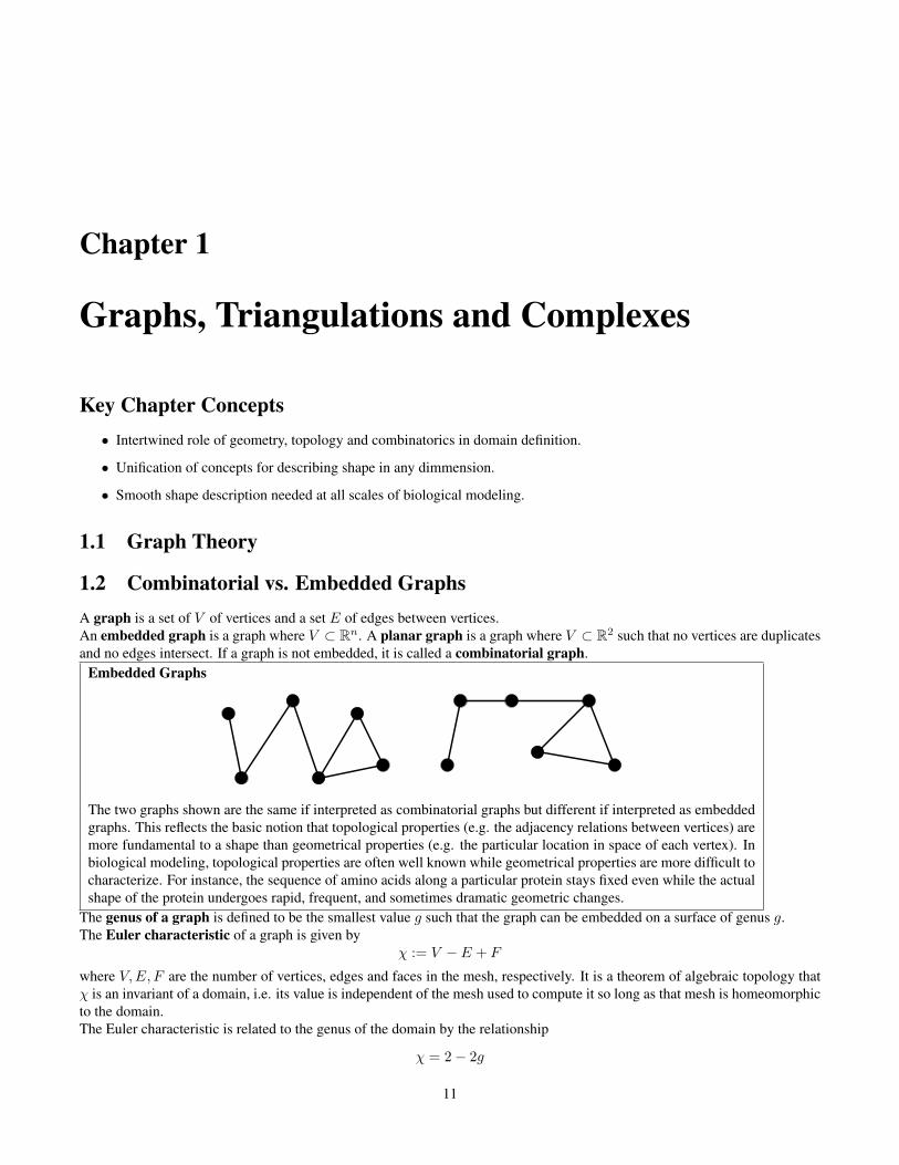
1.2 Combinatorial vs. Embedded GraphsA graph is a set of V of vertices and a set E of edges between vertices.An embedded graph is a graph where V ⊂ Rn. A planar graph is a graph where V ⊂ R2 such that no vertices are duplicatesand no edges intersect. If a graph is not embedded, it is called a combinatorial graph.
Embedded Graphs
The two graphs shown are the same if interpreted as combinatorial graphs but different if interpreted as embeddedgraphs. This reflects the basic notion that topological properties (e.g. the adjacency relations between vertices) aremore fundamental to a shape than geometrical properties (e.g. the particular location in space of each vertex). Inbiological modeling, topological properties are often well known while geometrical properties are more difficult tocharacterize. For instance, the sequence of amino acids along a particular protein stays fixed even while the actualshape of the protein undergoes rapid, frequent, and sometimes dramatic geometric changes.
The genus of a graph is defined to be the smallest value g such that the graph can be embedded on a surface of genus g.The Euler characteristic of a graph is given by
χ := V − E + F
where V,E, F are the number of vertices, edges and faces in the mesh, respectively. It is a theorem of algebraic topology thatχ is an invariant of a domain, i.e. its value is independent of the mesh used to compute it so long as that mesh is homeomorphicto the domain.The Euler characteristic is related to the genus of the domain by the relationship
χ = 2− 2g
11

12 CHAPTER 1. GRAPHS, TRIANGULATIONS AND COMPLEXES
1.2.1 Network Theory
A direceted graph is a graph whose edges have a specific orientation. A flow network is a directed graph where each edgealso has a capacity.
Max Cut Min Flow Theorem A flow network can be thought of as a highway system with only one-way streets.Vertices represent locations and edges represent the streets between them. The direction of an edge indicates whichway traffic is allowed to travel on that street. The capacity of an edge represents the maximum traffic that can flowdown the street at any one moment (e.g. the number of lanes in the road).The Max Cut Min Flow Theorem states that in a flow network, the maximum amount of flow passing from a sourceto a sink is equal to the minimum capacity which when removed in a specific way from the network causes thesituation that no flow can pass from the source to the sink. It is a formalization and generalization of the familiarnotion that a chain is only as strong as its weakest link.
1.2.2 Trees and Spanning Trees
Minimal spanning trees, etc.
1.3 Topological Complexes
1.3.1 Pointset Topology
Let S be a set and let T be a family of subsets of S. Then T is called a topology on S if
• Both the empty set and S are elements of T .
• Any union of arbitrarily many elements of T is an element of T .
• Any intersection of finitely many elements of T is an element of T .
If T is a topology on S, then the pair (S, T ) is called a topological space. If the topology is implicit, the space S is listedwithout mention of T .
The members of T are called the open sets of S. A set is called closed if its complement is in T .
A neighborhood of a point x ∈ S is any element of T containing x.
We will often deal with subsets of Rn with the usual topology. This means the set S is the points of Rn and the T is formedfrom all open balls of any radius in Rn.

1.3. TOPOLOGICAL COMPLEXES 13
Manifolds
sphere torus half sphere
A manifold is a special kind of topological space commonly used in domain modeling. At any point x in an n-manifold M , there exists a neighborhood of x which is homeomorphic to Rn. Thus the surface of a sphere, thesurface of a cube and the surface of a torus are all examples both 2-manifolds.If the manifold has boundary, then its boundary is described by those points which only have neighborhoodshomeomorphic to Rn−1.In the figure, the sphere and torus have genus 1 and 2, respectively. The half sphere is an example of a 2-manifoldwith boundary.
1.3.2 CW-complexesA Hausdorff space is a topological space in which distinct points have disjoint neighborhoods.
Definition 1.1. A CW-complex is a Hausdorff space X together with a partition of X into open cells of varying dimensionsuch that
1. For each n-dimensional open cell C in the set X , there exists a continuous map f from the n-dimensional closed ball toX such that the restriction of f onto the interior of the ball is a homeomorphism onto the cell C.
2. The image of the boundary of the open ball (i.e. the boundary of the open cell C) intersects only finitely many other cells.
A CW-complex can be presented as a sequence of spaces and maps
X0 → X1 → . . . → Xn → . . .
where each space Xn, called the n-dimensional skeleton of the presentation, is the result of attaching copies of the n-diskDn := x ∈ Rn : ||x|| ≤ 1 along their boundaries Sn−1 := ∂Dn to Xn−1.A Voronoi decomposition is a special kind of the more general class of CW-complexes.
Computational HomologyTriangulationas and CW-complexes can be used to compute the homology groups of a manifold, a topologicalinvariant. The ranks of these groups are called the Betti numbers, a simple and geometrically meaninful topologicalinvariant. We will discuss this further in Section 1.4.1.
1.3.3 Morse Functions and the Morse-Smale ComplexMorse theory(Adding a citation here) provides useful results not only for the construction of contour trees but also for anevaluation of the smooth distance function hΣ defined at the end of Section 1. As in the previous section, we consider a smoothfunction f : M → R1, now adding the restriction that M is a compact 3-manifold without boundary. Let m ∈ M be anon-degenerate critical point of f , meaning the derivative map dfm is the zero map and the Hessian at m is non-singular. We

14 CHAPTER 1. GRAPHS, TRIANGULATIONS AND COMPLEXES
note that a critical point m lies in the domain M of f as opposed to a critical value r which lies in the range R1 of f . TheMorse Lemma [84] states that f exhibits quadratic behavior in a small neighborhood m. That is, we may choose a coordinatechart about m such that locally
f(x, y, z) = f(m)± x2 ± y2 ± z2
We define the index of m to be the number of minus signs in the equation above. It can be shown that the index is independentof the coordinate chart and that it is equal to the number of negative eigenvalues of the Hessian at m.Thus, in three dimensions, a non-degenerate critical point can have index 0, 1, 2, or 3. These indices correspond to minima,1-saddles, 2-saddles, and maxima of the function f , respectivelyWe can unambiguously connect these critical points into a meaningful structure known as the Morse complex. Away fromcritical points, the gradient vector ∇f is non-zero and points in the direction of maximum positive change. If we construct amaximal path whose velocity vectors coincide with the gradient vector at each point on the path, we will always connect twocritical points. Such a path is called an integral path and necessarily terminates at a critical point of index 1, 2, or 3. We definethe stable manifold of a non-degenerate critical point m ∈ M to be the union of m and the images of all integral paths on Mterminating at m. We note that an unstable manifold can be defined similarly, but we will not need it in this paper.(Criticalinconsistency, changes shall be made here) For our purposes, the Morse Complex is defined to be the union of all maxima andtheir stable manifolds.Previous work employing the Morse complex has dealt primarily with two types of input functions: grids and surfaces. Thecomplex has been defined on two-dimensional grids and three-dimensional unstructured tetrahedral grids by Edelsbrunner, etal. [42, 41]. Cazals, Chazal and Lewiner used the Morse complex for molecular shape analysis in [24]. As described in Section3, our work uses the Morse complex to aid in the curation of molecular surfaces.Upper left: critical points (minima, saddle points and maxima pictured as blue, green and red disks), and three integral lines(pink curves) of a Morse function. Black arrows show the gradient of that function. Upper right: ascending 2-manifolds :the set of points belonging to integral lines whose destination is the same minimum (critical point of index 0). Lower left:descending 2-manifolds : the set of points belonging to integral lines whose origin is the same maximum (critical point ofindex 2). Lower right: the Morse-Smale complex : a natural tesselation of space into cells induced by the gradient fo thefunction. Each cell is the set of points belonging to integral lines whose origin and destination are identical (i.e. each cell isthe intersection of an ascending and a descending manifold). The purple region is a 2-cell: intersection of an ascending anda descending 2-manifold (red and blue regions) where all field lines have the same orgin and destination (a minimum and amaxium). The yellow curve is a 1-cell (also called an arc): the intersection of and ascending 2-manifold (blue region) and adescending 1-manifolds (green+yellow curves, originating from the same saddle point).
1.3.4 Signed Distance Function and Critical Points of Discrete Distance FunctionsIt seems that this paragraph is cited from somewhere, what is the citation reference? (yiwang)The key ingredient in ranking the topological features of the extracted level set is the distance function over R3. The distancefunction has been used earlier for reconstruction and image feature identification [8, 25, 39, 54, 119]. Chazal and Lieutier [27]have used it for stable medial axis construction. Dey, Giesen and Goswami have used distance function for object segmentationand matching [36]. Goswami, Dey and Bajaj have used it for detailed feature analysis of shape via an annotation of flat andtubular features in addition to shape segmentation [55]. Recently, Bajaj and Goswami have shown a novel use of distancefunction, induced by a molecular surface, in order to detect secondary structural motifs of a protein molecule [10]. The closeconnection between the critical point structure of the distance function and the topology of the surface and its complement iswhat we utilize to detect and remove small topological artifacts.In this context, Σ is the extracted isosurface. For the ease of computation, we approximate hΣ by hP which assigns to everypoint in R3, the distance to the nearest point from the set P which finitely samples Σ.
hP : R3 → R, x 7→ minp∈P‖x− p‖
With our extracted isosurface, we make use of the distance function introduced above. Given a compact surface Σ smoothlyembedded in R3, a distance function hΣ can be designed over R3 that assigns to each point its distance to Σ.
hΣ : R3 → R, x 7→ infp∈Σ‖x− p‖

1.3. TOPOLOGICAL COMPLEXES 15
Figure 1.1: Upper left: critical points (minima, saddle points and maxima pictured as blue, green and red disks), and threeintegral lines (pink curves) of a Morse function. Black arrows show the gradient of that function. Upper right: ascending2-manifolds : the set of points belonging to integral lines whose destination is the same minimum (critical point of index 0).Lower left: descending 2-manifolds : the set of points belonging to integral lines whose origin is the same maximum (criticalpoint of index 2). Lower right: the Morse-Smale complex : a natural tesselation of space into cells induced by the gradientfo the function. Each cell is the set of points belonging to integral lines whose origin and destination are identical (i.e. eachcell is the intersection of an ascending and a descending manifold). The purple region is a 2-cell: intersection of an ascendingand a descending 2-manifold (red and blue regions) where all field lines have the same orgin and destination (a minimum anda maxium). The yellow curve is a 1-cell (also called an arc): the intersection of and ascending 2-manifold (blue region) and adescending 1-manifolds (green+yellow curves, originating from the same saddle point).

16 CHAPTER 1. GRAPHS, TRIANGULATIONS AND COMPLEXES
We identify the maxima and index 2 saddle points of hP which lie outside the level set. The stable manifolds of these criticalpoints help detect the tunnels and the pockets of Σ. Additionally, these stable manifolds are used to compute geometricattributes of the detected topological features to which they correspond. In this way, we obtain a description of the isosurface,and its complement, in terms of its topological features. These features are quantified by their geometric properties and may beselectively removed.The function hP induces a flow at every point x ∈ R3 and this flow has been characterized earlier [54, 55]. See also [39].The critical points of hP are those points where hP has no non-zero gradient along any direction. These are the points in R3
which lie within the convex hull of its closest points from P . It was shown by Siersma [104] that the critical points of hP arethe intersection points of the Voronoi objects with their dual Delaunay objects.
• Maxima are the Voronoi vertices contained in their dual tetrahedra,
• Index 2 saddles lie at the intersection of Voronoi edges with their dual Delaunay triangles,
• Index 1 saddles lie at the intersection of Voronoi facets with their dual Delaunay edges, and
• Minima are the sample points themselves as they are always contained in their Voronoi cells.
In this discrete setting, the index of a critical point is the dimension of the lowest dimensional Delaunay simplex that containsthe critical point.At every x ∈ R3, a unit vector can be assigned that is oriented in the direction of the steepest ascent of hP . The critical pointsare assigned zero vectors. This vector field, which may not be continuous, nevertheless induces a flow in R3. This flow tellshow a point x moves in R3 along the steepest ascent of hP and the corresponding path is called the orbit of x.For a critical point c its stable manifold is the set of points whose orbits end at c. The stable manifold of a maximum is athree dimensional polytope whose boundary is composed of the stable manifolds of the index 2 saddle points which in turn arebounded by the stable manifolds of index 1 saddle points and minima. See [36, 54] for the detailed discussion on the structureand computation of the stable manifolds of the critical points of hP .
1.3.5 Contouring Tree Representation
1.4 Complementary space topology and geometry
Compactifying Complementary SpaceA molecular surface S bounds a finte portion of R3, viz. the interior volume V of the molecule. The comple-mentary space, defined to be R3 − V , contains useful geometric and topological information about the surfacesuch as the number of connected components and number of tunnels passing through the surface. Since R3 − Vis unbounded, we compactify complementary space to get a handle on these features by using some results fromMorse theory.
We construct an approximation of the Morse complex for hΣ described in Section 1.3.4 based on the critical points known forhP . First we describe the classification of the requisite critical points and then describe how they are clustered together. Thecritical points of hP are detected by checking the intersection of the Voronoi and its dual Delaunay diagram of the point setP sampled from Σ. The critical points are primarily of three types depending on if the Voronoi/Delaunay object involved liesinterior to Σ, exterior to Σ, or if the Voronoi object crosses Σ. There are some exceptions: maxima can not lie on the surfaceand therefore come in only two types - interior and exterior. The minima are sample points themselves and therefore they arealways on Σ. The saddle points can be any of three types mentioned above.Since the Morse complex we construct requires only the maxima and index 2 saddles exterior to or on the surface Σ, we fixthree classes of critical points:
C2,E = index 2 saddles of hP exterior to ΣC2,S = index 2 saddles of hP on the surface ΣC3,E = maxima of hP exterior of to Σ
We include a point at infinity denoted (m∞) in the set C3,E to compactify the copmlementary space structure.

1.4. COMPLEMENTARY SPACE TOPOLOGY AND GEOMETRY 17
As discussed in previous section, the points in the above classes come with a natural hierarchical structure based on stablemanifolds. We construct a graph on the points based on this structure by the following rule: a maxima m ∈ C3,E is connectedto a saddle s ∈ C2,E ∪ C2,S if and only if the stable manifold of s lies on the boundary of the stable manifold of m. We usethis graph to detect tunnels and pockets. The algorithm is depicted visually in Figure 1.2.
(a) (b) (c)
Figure 1.2: A visual depiction of our tunnel and pocket detection algorithm. An imaginary molecular surface is shown with a3-mouth tunnel and a single pocket. (a) Critical points of hP are detected. Blue points are index 2 saddles and brown pointsare maxima. (b) A point at infinity is added and a graph constructed based on adjacency of stable manifolds. This graphapproximates the Morse complex. (c) Breaking the edges to the point at infinity, we detect the tunnel (yellow with red mouths)and pocket (green with purple mouth).
1.4.1 Detection of Tunnels and PocketsWe first show that the graph constructed on the critical points of hP has B0 + 1 components where B0 is the 0-th Betti number.Any critical point inside a tunnel or pocket of the surface will have a path along the graph to m∞, the maximum at infinity.This reflects the fact that there is, by definition, a “way out” from a tunnel or pocket. A critical point in a void, on the otherhand, will not have a path to m∞ and thus lies in a component separate from the tunnels and pockets. Since B0 equals thenumber of voids captured by the surface, the graph has exactly B0 + 1 components. Hence, the voids of Σ are precisely thestable manifolds of the components not containing m∞.With the component of the graph containing m∞, we cluster it into tunnels and pockets as follows. Observe that the point m∞is connected only to index 2 saddles that lie on the mouth of a tunnel or pocket. Therefore, by “chopping around” the pointm∞, we break apart the graph based on tunnels and pockets. More precisely, let C2,∞ ⊂ C2,E ∪ C2,S denote the set of pointsconnected to m∞. Removing all the edges from the point m∞, we are left with n components of the graph, one correspondingto each tunnel or pocket of Σ. The stable manifolds of the points of C2,∞ form the mouths of the tunnels and pockets and wecan now classify all components of our modified graph as follows.
• 0 Mouth indicates that the component belongs to a void.
• 1 Mouth indicates that the component belongs to a pocket.
• k ≥ 2 Mouths indicate the component belongs to a tunnel. We call it a k-mouthed tunnel.
We use the algorithms described in [54] for computation of the stable manifolds of index 2 saddles. In order to have a compu-tational description of the detected features, we also compute the stable manifolds of the maxima falling into every componentusing the algorithm described in [36]. This produces a tetrahedral decomposition of the features captured.

18 CHAPTER 1. GRAPHS, TRIANGULATIONS AND COMPLEXES
Contour TreeIsocontour Selection
Figure 1.3: Results: Top row shows the interface selection for Rieske Iron-sulphur Protein molecule (PDB ID: 1RIE) from ablurred density map. Bottom row shows the isosurface selection for the virus particle (GroEL) from cryo-EM density map.
We compute the pockets, tunnels and voids of the molecular surface. The tetrahedral solids describing the pockets and tunnelsprovide a nice handle to those features and using these handles, the features can be ranked. We primarily use the geometricattributes of the features in order to rank them. Such attributes include, but are not limited to, the combined volume of thetetrahedra and the area of the mouths. The pockets and tunnels are then sorted in order of their increasing geometricallymeasured importance.Removal of insignificant features are also made easy because of the volumetric description of the features. As dictated by theapplications, a cut-off is set below which the features are considered noise. We remove the topological noise by marking theoutside tetrahedra as inside and updating the surface triangles.We show the results of our algorithm on two volumetric data. The top row in Figure 1.3 shows the electron density volume ofRieske Iron-Sulphur Protein (Protein Data Bank Id: 1RIE). The volume rendering using VolRover [33] is shown in the leftmostsubfigure. The tool additionally supports the visualization and isosurface selection using CT. The other subfigures show theselected interface and the detected tunnels and pockets. Note, the mouth of the tunnel is drawn in red and the mouth of thepocket is drawn in purple. The rest of the tunnel surface is drawn in yellow while the pocket surface is drawn in green. Theblue patches in the rightmost subfigure shows the filling of the smaller tunnels and pockets. The second row shows the resultson the three dimensional scalar volume representing the electron density of the reconstructed image of a virus (GroEL) from aset of two dimensional electron micrographs. The resolution is 8rA.Using VolRover, a suitable level set is chosen. Note the CT is very noisy and has many branches, because of which it is notpossible to extract a single-component isosurface. Nevertheless only one component is vital and the rest of them are merelyartifacts caused by noise. The main component along with the detected tunnel is shown next. The result is particularly usefulin visualizing the symmetric structure of the virus particle as depicted in the symmetric set of mouths. In addition to detectingthe principal topological feature, the algorithm detects few small tunnels and pockets which are shown separately for visualclarity (rightmost subfigure) and these are removed subsequently as part of the topological noise removal process. (Suggestion:Remove this paragraph)However, so far we have discussed about curating the molecular surface by modifying only the complementary space topolog-ical features. This does not always serve the purpose. Consider a very thin interior surrounding a wide tunnel. The tunnel issignificant but the thin portion surrounding it should disappear which we have not taken into account so far. Figure 1.4 showsa similar scenario where the inherent symmetry of the 3D map of nodavirus is shown in subfigure (a). Subfigure (b) shows that

1.4. COMPLEMENTARY SPACE TOPOLOGY AND GEOMETRY 19
(a)(b)
(d)(c)
Figure 1.4: Identification of “thin” regions in the primal space. (a) The volume rendering of 3D image of nodavirus. (b) Tunnelsare detected for the initial selection of the isosurface. Note, in some places of 5-fold symmetry, only 4 mouths of the tunnelare present. (c) The thin regions (blue) are identified as subsets of the unstable manifolds of the index 1 saddles identifiedon the interior medial axis. The arrow between (b) and (c) indicate that the places where the 5th mouth of the tunnel shouldopen indeed have thin regions. (d) The final selected isosurface has complementary space topology consistent with the inherentsymmetry of the 3D map.

20 CHAPTER 1. GRAPHS, TRIANGULATIONS AND COMPLEXES
due to wrong choice of isovalue only 4 mouths are open in the complementary space tunnel of a 5-fold symmetric region. Tocurate this surface, modification of the complementary space is not sufficient. To deal with such cases, we extend the curationprocess by detecting “thin” regions in the primal space.Remarkably, distance function plays a very important role here also. In order to detect the thin regions, we first compute theinterior medial axis by publicly available software [30]. Further we compute the index 1 (U1)and index 2 (U2) saddle pointswhich lie on the interior medial axis and compute their unstable manifols using the algorithm described in [55]. U2 produceslinear subset of the medial axis and U1 produces planar subset of the medial axis. We then sample the distance function on U1
and U2 and identify the subset corresponding to the “thin” regions measured by a suitable threshold parameter. Figure 1.4 (c)shows the thin regions (blue patches) on the U1 (green) identified for noda virus. The reason for not using medial axis directlyis that medial axis tends to be noisy and U1 and U2 usually describes the subset of the medial axis stable against the smallundulation on the surface. Then we collect the interior maxima falling into the thin subset of U1 and U2 and compute theirstable manifolds. Again, the stable manifolds are the collection of tetrahedra and therefore we cut the surface open by forminga channel interior to the volume bounded by the molecular surface by appropriately toggling the marking of the tetrahedra frominside to outside. Final selection of the isosurface for which the mouths of the tunnels respect the inherent symmetry of thedensity map of the virus is shown in Figure 1.4 (d).
1.5 Primal and Dual Complexes
1.5.1 Primal MeshesIn algebraic topology, manifolds are discretized using simplicial complexes, a notion which guides the entire theory of discreteexterior calculus. We state the definition of simplicial complex here, along with supporting definitions to be used throughout.
Definition 1.2. A k-simplex σk is the convex hull of k + 1 geometrically independent points v0, . . . , vk ∈ RN . Any simplexspanned by a (proper) subset of v0, . . . , vk is called a (proper) face of σk. The union of the proper faces of σk is calledits boundary and denoted Bd(σk). The interior of σk is Int(σk) = σk\Bd(σk). Note that Int(σ0)=σ0. The volume of σk isdenoted |σk|. Define |σ0 |= 1. ♦
Primal Simplicies
Primal simplices of dimension 0, 1, 2, and 3 are shown. In general, a k-simplex is the convex hull of k points inRn in general position. We denote a k-simplex as σk.
We will indicate that a simplex has dimension k with a superscript, e.g. σk, and will index simplices of any dimension withsubscripts, e.g. σi.
Definition 1.3. A simplicial complex K in RN is a collection of simplices in RN such that
1. Every face of a simplex of K is in K.
2. The intersection of any two simplices of K is either a face of each of them or it is empty.
The union of all simplices of K treated as a subset of RN is called the underlying space of K and is denoted by |K|. ♦
Definition 1.4. A simplicial complex of dimension n is called a manifold-like simplicial complex if and only if |K| is aC0-manifold, with or without boundary. More precisely,
1. All simplices of dimension k with 0 ≤ k ≤ n− 1 must be a face of some simplex of dimension n in K.
2. Each point on |K| has a neighborhood homeomorphic to Rn or n-dimensional half-space. ♦

1.5. PRIMAL AND DUAL COMPLEXES 21
Remark 1.5. Since DEC is meant to treat discretizations of manifolds, we will assume all simplicial complexes are manifold-like from here forward. We note that |K| is thought of as a piecewise linear approximation of a smooth manifold Ω. Formally,this is taken to mean that there exists a homeomorphism h between |K| and Ω such that h is isotopic to the identity. Inapplications, however, knowing h or Ω explicitly may be irrelevant or impossible as K often encodes everything known aboutΩ. This emphasizes the usefulness of DEC as a theory built for discrete settings. ♦
Orientation of Simplicial Complexes We now review how to orient a simplicial complex K.
Definition 1.6. Define two orderings of the vertices of a simplex σk (k ≥ 1) to be equivalent if they differ by an evenpermutation. Thus, there are two equivalence classes of orderings, each of which is called an orientation of σk. If σk is writtenas [v0, . . . , vk], the orientation of σk is understood to be the equivalence class of this ordering. ♦
Definition 1.7. Let σk = [v0, . . . , vk] be an oriented simplex with k ≥ 2. This gives an induced orientation on each of the(k− 1)-dimensional faces of σk as follows. Each face of σk can be written uniquely as [v0, . . . , vi, . . . , vk], where vi means viis omitted. If i is even, the induced orientation on the face is the same as the oriented simplex [v0, . . . , vi, . . . , vk]. If i is odd,it is the opposite. ♦
We note that this formal definition of induced orientation agrees with the notion of orientation induced by the boundary operator(Definition 4.12). In that setting, a 0-simplex can also receive an induced orientation.Remark 1.8. We will need to be able to compare the orientation of two oriented k-simplices σk and τk. This is possible only ifat least one of the following conditions holds:
1. There exists a k-dimensional affine subspace P ⊂ RN containing both σk and τk.
2. σk and τk share a face of dimension k − 1.
In the first case, write σk = [v0, . . . , vk] and τk = [w0, . . . , wk]. Note that v1−v0, v2−v0, . . . , vk−v0 and w1−w0, w2−w0, . . . , wk − w0 are two ordered bases of P . We say σk and τk have the same orientation if these bases orient P the sameway. Otherwise, we say they have opposite orientations. In the second case, σk and τk are said to have the same orientation ifthe induced orientation on the shared k − 1 face induced by σk is opposite to that induced by τk. ♦
Definition 1.9. Let σk and τk with 1 ≤ k ≤ n be two simplices whose orientations can be compared, as explained in Remark1.8. If they have the same orientation, we say the simplices have a relative orientation of +1, otherwise −1. This is denotedas sgn(σk, τk) = +1 or −1, respectively. ♦
Definition 1.10. A manifold-like simplicial complexK of dimension n is called an oriented manifold-like simplicial complexif adjacent n-simplices agree on the orientation of their shared face. Such a complex will be called a primal mesh from hereforward. ♦
1.5.2 Dual ComplexesDual complexes are defined relative to a primal mesh. While they represent the same subset of RN as their associated pri-mal mesh, they create a different data structure for the geometrical information and become essential in defining the variousoperators needed for DEC.
Dual Cells
Dual cells of dimension 0, 1, 2, and 3 are shown. In general, a k-cell is the convex hull of k points in Rnhomeomorphic to a filled k-ball such that the boundary of the k-cell is a collection of k − 1 cells. If a k-cell isdefined as the dual of an n− k simplex, we denote it as ?σn−k.
22 CHAPTER 1. GRAPHS, TRIANGULATIONS AND COMPLEXES
Definition 1.11. The circumcenter of a k-simplex σk is given by the center of the unique k-sphere that has all k+1 vertices ofσk on its surface. It is denoted c(σk). A simplex σk is said to be well-centered if c(σk) ∈ Int(σk). A well-centered simplicialcomplex is one in which all simplices (of all dimensions) in the complex are well-centered. ♦
Definition 1.12. Let K be a well-centered primal mesh of dimension n and let σk be a simplex in K. The circumcentric dualcell of σk, denoted D(σk), is given by
D(σk) :=
n−k⋃r=0
⋃σk≺σ1≺···≺σr
Int(c(σk)c(σ1) . . . c(σr)).
To clarify, the inner union is taken over all sequences of r simplices such that σk is the first element in the sequence and eachsequence element is a proper face of its successor. Hence, σ1 is a (k + 1) simplex and σr is an n simplex. For r = 0, this is tobe interpreted as the sequence σk only. The closure of the dual cell of σk is denoted D(σk) and called the closed dual cell. Wewill use the notation ? to indicate dual cells, i.e.
?σ := D(σ).
Each (n−k)-simplex on the points c(σk), c(σ1), . . . , c(σr) is called an elementary dual simplex of σk. The collection of dualcells is called the dual cell decomposition of K and denoted D(K) or ?K. ♦
Note that the dual cell decomposition forms a CW complex.
Orientation of Dual Complexes Orientation of the dual complex must be done in a such a way that it “agrees” with theorientation of the primal mesh. This can be done canonically since a primal simplex and any of its elementary dual simpliceshave complementary dimension and live in orthogonal affine subspaces of RN . We make this more precise and fix the necessaryconventions with the following definitions.
Definition 1.13. Let K be a primal mesh containing a sequence of simplices σ0 ≺ σ1 ≺ · · · ≺ σn and let σk be one ofthese simplices with 1 ≤ k ≤ n − 1. The orientation of the elementary dual simplex with vertices c(σk), . . . , c(σn) iss[c(σk), . . . , c(σn)] where s ∈ −1,+1 is given by the formula
s := sgn([c(σ0), . . . , c(σk)], σk
)× sgn
([c(σ0), . . . , c(σn)], σn
).
The sgn function was defined in Definition 1.9.For k = n, the dual element is a vertex which has no orientation. For k = 0, define s := sgn
([c(σ0), . . . , c(σn)], σn
). ♦
The above definition serves to orient all the elementary dual simplices associated to σk and hence all simplices in a dual celldecomposition. Further, the orientations on the elementary dual simplices induce orientations on the boundaries of dual cellsin the same manner as given in Definition 1.7. The induced orientations on adjacent (n− 1) cells will agree since the dual celldecomposition comes from a primal mesh (see Definition 1.10).
Definition 1.14. The oriented dual cell decomposition of a primal mesh is called the dual mesh. ♦
1.6 Voronoi and Delaunay Decompositions
For a finite set of points P in R3, the Voronoi cell of p ∈ P is
Vp = x ∈ R3 : ∀q ∈ P − p, ‖x− p‖ ≤ ‖x− q‖).
If the points are in general position, two Voronoi cells with non-empty intersection meet along a planar, convex Voronoi facet,three Voronoi cells with non-empty intersection meet along a common Voronoi edge and four Voronoi cells with non-emptyintersection meet at a Voronoi vertex. A cell decomposition consisting of the Voronoi objects, that is, Voronoi cells, facets,edges and vertices is the Voronoi diagram VorP of the point set P .

1.6. VORONOI AND DELAUNAY DECOMPOSITIONS 23
Voronoi and Delaunay Meshes
Voronoi and Delaunay meshes are dual decompositions of the same domain. In the figure, the small red dots definethe Voronoi cells and hence a dual mesh of the domain (shown at right) but also define the vertices of the Delaunaytriangles and hence a primal mesh of the domain (shown at left).
The dual of VorP is the Delaunay diagram DelP of P which is a simplicial complex when the points are in general position.The tetrahedra are dual to the Voronoi vertices, the triangles are dual to the Voronoi edges, the edges are dual to the Voronoifacets and the vertices (sample points from P ) are dual to the Voronoi cells. We also refer to the Delaunay simplices as Delaunayobjects.
1.6.1 Euclidean vs. Power distance.
For MVC the choice of using the Power distance in place of the Euclidean distance is motivated by the the efficiency andsimplicity of the construction of the power diagram together with the fact that the power distance can be proven to be an upperbound of the Euclidean distance.
Consider a point p at distance d from the center c a ball B of radius r as in Figure 1.5. We define:
E(p,B) = |d− r| , P (p,B) =√|d2 − r2| .
Then we have the following chain of inequalities (where r and d are positive numbers):
0 ≤ 4dr(d− r)2 = 4d3r − 8d2r2 + 4dr3
(d− r)4 = d4 − 4d3r + 6d2r2 − 4dr3 + r4
≤ d4 − 2d2r2 + r4 = (d2 − r2)2
E(p,B) = |d− r| ≤√|d2 − r2| = P (p,B) .

24 CHAPTER 1. GRAPHS, TRIANGULATIONS AND COMPLEXES
(a) (b)
Figure 1.5: Relationship between the Euclidean distance E(p,B) between the point p and the ball B and their Power distanceP (p,B), (a) Configuration for d > r. (b) Configuration for d < r.
If the point p is outside the ball B the following inequality holds (both r and d are positive numbers):
r < d
r − d ≤ 0
2r2 − 2rd ≤ 0
2r2 − 2rd+ d2 ≤ d2
r2 − 2rd+ d2 ≤ d2 − r2
(r − d)2 ≤ d2 − r2
(r − d) ≤√d2 − r2
E(p,B) ≤ P (p,B)
That is the P (p,B) is larger than the Euclidean distance E(p,B) . The same relation holds if p is inside B:
d ≤ r
d− r ≤ 0
2d2 − 2rd ≤ 0
2d2 − 2rd+ r2 ≤ r2
d2 − 2rd+ r2 ≤ r2 − d2
(d− r)2 ≤ r2 − d2
(d− r) ≤√r2 − d2
E(p,B) ≤ P (p,B)
In conclusion we have that for any given ball B and point p, the function P (p,B) provides an upper bound on the distanceE(p, b):
E(p,B) ≤ P (p,B) , (1.1)
with equality holding only when d = r, i. e. the point is on the surface of the ball (and in trivial cases where d or r is zero).For a collection of n balls B = B1, . . . , Bn the distance functions are extended as follows:
E(p,B) = min1≤i≤n
|di − ri| (1.2)

1.6. VORONOI AND DELAUNAY DECOMPOSITIONS 25
P (p,B) =√
min1≤i≤n
|d2i − r2
i | (1.3)
The problem in comparing E(p,B) with P (p,B) is that they may achieve their minimum for different values of i because ingeneral the Power diagram is not coincident with the Voronoi diagram. Figure 1.6.1 shows an example of comparison betweenthe Voronoi diagram of two circles (in red) with the corresponding Power diagram (in blue). In this example the minimumdistance of the point p from the set B = B1, B2 is achieved at i = 1 for P (p,B) and at i = 2 for E(p,B):
P (p,B) = P (p,B1)
E(p,B) = E(p,B2) .
In general for a given point p we call iP , iE the two indices such that:
P (p,B) = P (p,BiP )
E(p,B) = E(p,BiE ) .
From equations (1.2) and (1.1) we have that:
E(p,B) = E(p,BiE ) ≤ E(p,BiP )
≤ P (p,BiP ) = P (p,B) .
(a) (b)
Figure 1.6: Power diagram (in blue) and Voronoi diagram (in red) of two circles. (a) Case of nonintersecting circles. (b) Caseof intersecting circles.
1.6.2 Weighted Alpha Shapes
A simplex s in the regular triangulation of Pi belongs to the α-shape of Pi only if the orthogonal center of (the weightedpoint orthogonal to the vertices of) s is smaller than α. The alpha shape where α = 0, called the zero-shape, is the topologicalstructure of molecules. For example, an edge e = (u, v) is a part of the zero-shape only if ‖u − v‖2 − wu − wv < 0, whichmeans that the two balls centered at u and v intersect (Figure 1.7(d)).

26 CHAPTER 1. GRAPHS, TRIANGULATIONS AND COMPLEXES
(a) (b) (c) (d) (e) (f)
Figure 1.7: The combinatorial and geometric structures underlying a molecular shape: (a) The collection of balls (weightedpoints). (b) Power diagram of a set of the points. (c) Regular triangulation. (d) The α-shape (with α = 0) of the points. (e)Partitioning of the molecular body induced by the power diagram. (f) The boundary of the molecular body.
1.7 Biological Applications
1.7.1 Union of Balls Topology
Stereographic Projection
a b ca
b
c∞ ∞
∞
For any integer n ≥ 1, the space Rn ∪ ∞ can be mapped to the n-dimensional sphere, commonly denoted Sn
by a mapping called stereographic projection. In the 1D case shown above, the real line is mapped to the circleS1 by wrapping the points at infinity together to the top of the circle. The general form of the mapping is given by
s : Sn → Rn, (x1, . . . , xn+1)→ 1
1− xn+1(x1, . . . , xn)
with the convention (0, . . . , 1)→ ∞. This process can be used to wrap 2D power diagrams into 3D polytopes.
Power Diagram
Given a weighted point P = (p, wp) where p ∈ IRn and w ∈ IR, the power distance from a point x ∈ IRn to P is defined as
πP (x) =√‖p− x‖2 − wp ,
where ‖p− x‖ is the ordinary Euclidean distance between p and x.In molecule context, we define the weight of an atom B with center at p and radius r to be wB = r2. The power distance of xto B is
πB(x) =√‖p− x‖2 − r2 .
Given a set Pi of weighted vertices (each vertex has a weight wi associated with it), the Power Diagram is a tiling of thespace into convex regions where the ith tile is the set of points nearest to the vertex Pi, in the power distance metric The powerdiagram is similar to the Voronoi diagram using the power distance instead of Euclidean distance.The weighted Voronoi cell of a ball B in a molecule B is the set of points in space whose weighted distance to B is less than orequal to their weighted distance to any other ball in B:
VB = x ∈ IR2|πB(x) ≤ πC(x) ∀C ∈ B .
The power diagram of a molecule is the union of the weighted Voronoi cells for each of its atoms (Figure 1.7(b)).

1.7. BIOLOGICAL APPLICATIONS 27
Regular Triangulation
The regular triangulation, or weighted Delaunay triangulation, is the dual (face adjacency graph) of the power diagram, just asthe Delaunay triangulation is the dual shape of the Voronoi diagram. Vertices in the triangulation are connected if and only iftheir corresponding weighted Voronoi cells have a common face (Figure 1.7(c)). This implies that two vertices are connectedif and only if they have a nearest neighbor relation measured in power distance metricGiven a set of n 2D points with weights, it has been shown , that their regular triangulation can be computed in O(n log n)time, by incrementally inserting new points to the existing triangulation and correcting it using edge flips.
Wrapping the Power Diagram
We can model a union of balls as an embedded graph. If two balls intersect, their circle of intersection can be defined by threepoints. The arcs connecting these points are directed edges and can be parametrized as portions of a circle. Each face is portionof a sphere and the circular arcs defining its boundary. This can be captured compactly as a graph structure (vertices, edges,and faces).Moreover, the weighted Delaunay triangulation of the centers of the balls defines the topology of the volume. An edge inthe complex corresponds to two balls intersecting and a face (triangle) corresponds to three balls intersecting. A cycle of threeedges without a face corresponds to three balls which intersect pairwise but not mutually.We can wrap the weighted Delaunay diagram onto the 4-sphere using sterographic projection (see box). This mapping resultsin a polytope that compactly represents the union of balls topology and surface patch embedded graph.
1.7.2 Meshing of Molecular InterfacesIn this subsection, we describe an approach to generate quality triangular/tetrahedral meshes for complicated biomolecularstructures directly from the PDB format data, conforming to a good implicit solvation surface approximation. There are threemain steps in our mesh generation process:
1. Implicit Solvation Surface Construction – A smooth implicit solvation model is constructed to approximate the Lee-Richards molecular surface by using weighted Gaussian isotropic atomic kernel functions and a two-level clusteringtechniques.
2. Mesh Generation – A modified dual contouring method is used to extract triangular and interior/exterior tetrahedralmeshes, conforming to the implicit solvation surface. The dual contouring method is selected for mesh generation as ittends to yield meshes with better aspect ratio. In order to generate exterior meshes described by biophysical applications, we add a sphere or box outside the implicit solvation surface, and create an outer boundary. Our extracted tetrahedralmesh is spatially adaptive and attempts to preserve molecular surface features while minimizing the number of elements.
3. Quality Improvement – Geometric flows are used to improve the quality of extracted triangular and tetrahedral meshes.
The generated tetrahedral meshes of the monomeric and tetrameric mouse acetylcholinesterase (mAChE) have been success-fully used in solving the steady-state Smoluchowski equation using the finite element method .
Mesh Generation
There are two main methods for contouring scalar fields, primal contouring and dual contouring . Both of them can be extendedto tetrahedral mesh generation. The dual contouring method is often the method of choice as it tends to yield meshes withbetter aspect ratio.
Triangular Meshing Dual contouring uses an octree data structure, and analyzes those edges that have endpoints lyingon different sides of the isosurface, called sign change edges. The mesh adaptivity is determined during a top-down octreeconstruction. Each sign change edge is shared by either four (uniform case) or three (adaptive case) cells, and one minimizerpoint is calculated for each of them by minimizing a predefined Quadratic Error Function (QEF) :
QEF [x] =∑i
[ni · (x− pi)]2 , (1.4)

28 CHAPTER 1. GRAPHS, TRIANGULATIONS AND COMPLEXES
(a) (b) (c)
Figure 1.8: The analysis domain of exterior meshes. (a) - ‘O’ is the geometric center of the molecule, suppose the circum-sphere of the biomolecule has the radius of r. The box represents the volumetric data, and ‘S0’ is the maximum sphere insidethe box, the radius is r0(r0 > r). ‘S1’ is an outer sphere with the radius of r1(r1 = (20 ∼ 40)r). (b) - the diffusion domainis the interval volume between the molecular surface and the outer sphere ‘S1’, here we choose r1 = 5r for visualization. (c) -the outer boundary is a cubic box.
where pi, ni represent the position and unit normal vectors of the intersubsection point respectively. For each sign change edge,a quad or triangle is constructed by connecting the minimizers. These quads and triangles provide a ‘dual’ approximation ofthe isosurface.A recursive cell subdivision process was used to preserve the trilinear topology of the isosurface. During cell subdivision, thefunction value at each newly inserted grid point can be exactly calculated since we know the volumetric function. Additionally,we can generate a more accurate triangular mesh by projecting each generated minimizer point onto the isosurface.
Tetrahedral Meshing The dual contouring method has already been extended to extract tetrahedral meshes from volumetricscalar fields . The cells containing the isosurface are called boundary cells, and the interior cells are those cells whose eightvertices are inside the isosurface. In the tetrahedral mesh extraction process, all the boundary cells and the interior cells needto be analyzed in the octree data structure. There are two kinds of edges in boundary cells, one is a sign change edge, the otheris an interior edge. Interior cells only have interior edges. In [121, 122], interior edges and interior faces in boundary cells aredealt with in a special way, and the volume inside boundary cells is tetrahedralized. For interior cells, we only need to splitthem into tetrahedra.Adding an Outer Boundary In biological diffusion systems, we need to analyze the electrostatic potential field which isfaraway from the molecular surface . Assume that the radius of the circum-sphere of a biomolecule is r. The computationalmodel can be approximated by a field from an outer sphere S1 with the radius of (20 ∼ 40)r to the molecular surface. Thereforethe exterior mesh is defined as the tetrahedralization of the interval volume between the molecular surface and the outer sphereS1 (Fig. 1.8(b)).First we add a sphere S0 with the radius of r0 (where r0 > r and r0 = 2n/2 = 2n−1) outside the molecular surface, andgenerate meshes between the molecular surface and the outer sphere S0. Then we extend the tetrahedral meshes from thesphere S0 to the outer bounding sphere S1. For each data point inside the molecular surface, we keep the original functionvalue. While for each data point outside the molecular surface, we reset the function value as the smaller one of f(x)− α andthe shortest distance from the grid point to the sphere S0. Eqn. (1.5) shows the newly constructed function g(x) which providesa grid-based volumetric data containing the biomolecular surface and an outer sphere S0.
g(x) =
min(‖x− x0‖ − r0, f(x)− α), iff(x) < α, ‖x− x0‖ < r0,‖x− x0‖ − r0, iff(x) < α, ‖x− x0‖ ≥ r0,f(x)− α, iff(x) ≥ α,
(1.5)
where x0 are coordinates of the molecular geometric center. The isovalue α = 0.5 for volumetric data generated from thecharacteristic function, and α = 1.0 for volumetric data generated from the summation of Gaussian kernels.

1.7. BIOLOGICAL APPLICATIONS 29
The molecular surface and the outer sphere S0 can be extracted as an isosurface at the isovalue 0, Sg(0) = x|g(x) = 0. Allthe grid points inside the interval volume Ig(0) = x|g(x) ≤ 0 have negative function values, and all the grid points outsideit have positive values.
(a) (b)
Figure 1.9: 2D triangulation. (a) Old scheme, (b) New scheme. Blue and yellow triangles are generated for sign change edgesand interior edges respectively. The red curve represents the molecular surface, and the green points represent minimizer points.
Mesh ExtractionHere we introduce a different scheme from the algorithm presented in [121, 122], in which we do not distinguish boundarycells and interior cells when we analyze edges. We only consider two kinds of edges - sign change edges and interior edges.For each boundary cell, we can obtain a minimizer point by minimizing its Quadratic Error Function. For each interior cell,we set the middle point of the cell as its minimizer point. Fig. 1.9(b) shows a simple 2D example. In 2D, there are two cellssharing each edge, and two minimizer points are obtained. For each sign change edge, the two minimizers and the interiorvertex of this edge construct a triangle (blue triangles). For each interior edge, each minimizer point and this edge construct atriangle (yellow triangles). In 3D as shown in Fig. 1.10, there are three or four cells sharing each edge. Therefore, the three (orfour) minimizers and the interior vertex of the sign change edge construct one (or two) tetrahedron, while the three (or four)minimizers and the interior edge construct two (or four) tetrahedra.
Figure 1.10: Sign change edges and interior edges are analyzed in 3D tetrahedralization. (a)(b) - sign change edge (the rededge); (c)(d) - interior edge (the red edge). The green solid points represent minimizer points, and the red solid points representthe interior vertex of the sign change edge.
Compared with the algorithm presented in [121, 122] as shown in Fig. 1.9(a), Fig. 1.9(b) generates the same surface meshes,and tends to generate more regular interior meshes with better aspect ratio, but a few more elements for interior cells. Fig. 1.9(b)can be easily extended to large volume decomposition. For arbitrary large volume data, it is difficult to import all the data intomemory at the same time. So we first divide the large volume data into some small subvolumes, then mesh each subvolumeseparately. For those sign change edges and interior edges lying on the interfaces between subvolumes, we analyze themseparately. Finally, the generated meshes are merged together to obtain the desired mesh. The mesh adaptivity is controlled by
30 CHAPTER 1. GRAPHS, TRIANGULATIONS AND COMPLEXES
the structural properties of biomolecules. The extracted tetrahedral mesh is finer around the molecular surface, and graduallygets coarser from the molecular surface out towards the outer sphere, S0. Furthermore, we generate the finest mesh around theactive site, such as the cavity in the monomeric and tetrameric mAChE shown in Fig.?? (a∼b), and a coarse mesh everywhereelse.Mesh Extension
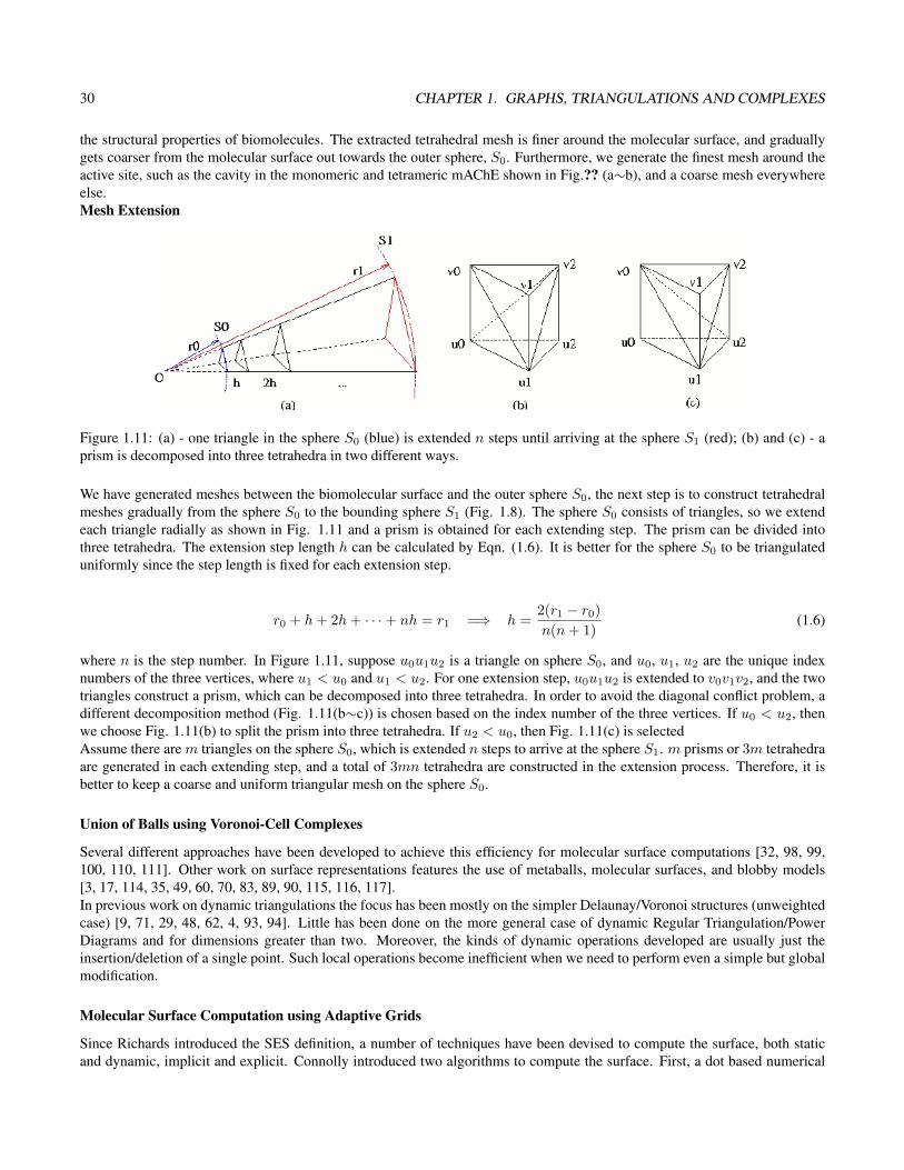
Figure 1.11: (a) - one triangle in the sphere S0 (blue) is extended n steps until arriving at the sphere S1 (red); (b) and (c) - aprism is decomposed into three tetrahedra in two different ways.
We have generated meshes between the biomolecular surface and the outer sphere S0, the next step is to construct tetrahedralmeshes gradually from the sphere S0 to the bounding sphere S1 (Fig. 1.8). The sphere S0 consists of triangles, so we extendeach triangle radially as shown in Fig. 1.11 and a prism is obtained for each extending step. The prism can be divided intothree tetrahedra. The extension step length h can be calculated by Eqn. (1.6). It is better for the sphere S0 to be triangulateduniformly since the step length is fixed for each extension step.
r0 + h+ 2h+ · · ·+ nh = r1 =⇒ h =2(r1 − r0)
n(n+ 1)(1.6)
where n is the step number. In Figure 1.11, suppose u0u1u2 is a triangle on sphere S0, and u0, u1, u2 are the unique indexnumbers of the three vertices, where u1 < u0 and u1 < u2. For one extension step, u0u1u2 is extended to v0v1v2, and the twotriangles construct a prism, which can be decomposed into three tetrahedra. In order to avoid the diagonal conflict problem, adifferent decomposition method (Fig. 1.11(b∼c)) is chosen based on the index number of the three vertices. If u0 < u2, thenwe choose Fig. 1.11(b) to split the prism into three tetrahedra. If u2 < u0, then Fig. 1.11(c) is selectedAssume there are m triangles on the sphere S0, which is extended n steps to arrive at the sphere S1. m prisms or 3m tetrahedraare generated in each extending step, and a total of 3mn tetrahedra are constructed in the extension process. Therefore, it isbetter to keep a coarse and uniform triangular mesh on the sphere S0.
Union of Balls using Voronoi-Cell Complexes
Several different approaches have been developed to achieve this efficiency for molecular surface computations [32, 98, 99,100, 110, 111]. Other work on surface representations features the use of metaballs, molecular surfaces, and blobby models[3, 17, 114, 35, 49, 60, 70, 83, 89, 90, 115, 116, 117].In previous work on dynamic triangulations the focus has been mostly on the simpler Delaunay/Voronoi structures (unweightedcase) [9, 71, 29, 48, 62, 4, 93, 94]. Little has been done on the more general case of dynamic Regular Triangulation/PowerDiagrams and for dimensions greater than two. Moreover, the kinds of dynamic operations developed are usually just theinsertion/deletion of a single point. Such local operations become inefficient when we need to perform even a simple but globalmodification.
Molecular Surface Computation using Adaptive Grids
Since Richards introduced the SES definition, a number of techniques have been devised to compute the surface, both staticand dynamic, implicit and explicit. Connolly introduced two algorithms to compute the surface. First, a dot based numerical

1.7. BIOLOGICAL APPLICATIONS 31
surface construction and second, an enumeration of the patches that make up the analytical surface (See [32], [31] and hisPhD thesis). In [111], the authors describe a distance function grid for computing surfaces of varying probe radii. Our datastructure contains approaches similar to their idea. A number of algorithms were presented using the intersection informationgiven by voronoi diagrams and the alpha shapes introduced by Edelsbrunner [43], including parallel algorithms in [110] and atriangulation scheme in [3]. Fast computations of SES is described in [99] and [98], using Reduced sets, which contains pointswhere the probe is in contact with three atoms, and faces and edges connecting such points. Non Uniform Rational BSplines( NURBs ) descriptions for the patches of the molecular surfaces are given in [12], [11] and [13]. You and Bashford in [118]defined a grid based algorithm to compute a set of volume elements which make up the Solvent Accessible Region.
Maintaining Union of Balls Under Atom Movements
Though a number of techniques have been devised for the static construction of molecular surfaces (e.g., [32, 31, 111, 43, 110, 3,99, 98, 118, 59, 12, 11, 123, 14]), not much work has been done on neighborhood data structures for the dynamic maintenanceof molecular surfaces as needed in MD. In [13] Bajaj et al. considered limited dynamic maintenance of molecular surfacesbased on Non Uniform Rational BSplines ( NURBS ) descriptions for the patches. Eyal and Halperin [45, 46] presented analgorithm based on dynamic graph connectivity that updates the union of balls molecular surface after a conformational changein O
(log2 n
)amortized time per affected (by this change) atom.
Clustering and Decimation of Molecular Surfaces
Using multiresolution models for molecules can substantially improve rendering speed and interactive response rates in molec-ular interaction tools. Similar improvements in performance would be achieved when a set of balls is used as an approximaterepresentation of a generic object either for modeling (meta-balls [60, 90], blobby models [117]) or for collision detection[70]. Direct application of previous approaches for the decimation and multiresolution representation of the surfaces them-selves [99, 77] can have serious embedding and self-intersection problems and are specific to the surface definition. A possiblesolution if this problem has been addressed in [108] but limited to the case of the boundary surface of tetrahedral meshes. Ourmultiresolution scheme updates the underlying structure of the molecule, maintaining at any level of detail a regular triangu-lation of the current weighted point-set. In this way we explicitly track the topology of the molecular body at any adaptivelevel of resolution. Moreover this guarantees correct embedding in all resolutions and creates an approximation from which thesurface boundary can be computed in any of the previous schemes.There are many approaches for creating multiresolution representations of geometric data for graphics and visualization [96,82, 75]. They vary in both the simplification scheme like vertex removal [34], edge contraction [68], triangle contraction [53],vertex clustering [102], wavelet analysis [37], and also in the structure used to organize the levels of detail (either a linear orderor a using a DAG).Maintaining the regular triangulation at all resolutions rules out the possibility of using decimation techniques like edge ortriangle contraction, which do not guarantee the (weighted) Delaunay property. Other known decimation schemes that canguarantee this property such as vertex removal, do not seem appropriate in this case since they do not preserve the moleculefeatures as a subset of the whole triangulation. Techniques which preserve features in the triangulation by tagging specific edgesor vertices [28] are more suitable for preserving specific edges or regions. We are more interested in applying the decimationon a subset of the triangulation while this subset can change during the decimation.Sphere trees have also been used in [69] for the purpose of fast collision detection. In this work, Sphere hierarchies are builtaround a given object either by replacing special octree regions or by placing balls on the medial-axis surfaces approximatedusing voronoi edges of some point sampling of the object. The basic approach of building the hierarchy by clustering pairsof balls for collision detection [70] is similar to ours. However in this scheme the simplification process does not update theunderlying triangulation and hence does not track the topological changes induced by the decimation process. This make alsothe scheme unable to cluster balls that get in contact only after some simplification steps.
Summary
References and Further Reading• Set theory background can be found in Rosen [95].

32 CHAPTER 1. GRAPHS, TRIANGULATIONS AND COMPLEXES
• Useful references for graph theory include Behzad and Chartrand [16], Chartrand and Lesniak [26], and Giblin [52]
• Minimal spanning trees are discussed in Graham and Hell [58] and algorithms for finding them in Kruskal[76]
• Useful algebraic topology texts include Armstrong [5] and Hatcher [64]. This includes more formal definitions of termslike homeomorphism, isomorphism, manifold, and homology.
• Some notation on primal and dual meshes has been adapted from Hirani [65].
• For practical computational topology, see Zomorodian [125]
• For more on CW complexes, see Munkres [86].
• The power distance metric is described in [7].
• More on regular triangulations in [40, 44] and on weighted alpha shapes in [38, 47].
• Some application references: [121, 122, 21, 22, 106, 107, 120, 73, 51, 67, 78].
Exercises

Chapter 2
Sets, Functions and Mappings
2.1 Scalar, Vector and Tensor FunctionsDefinition 2.1. We use the following basic definitions
• A scalar function is a function whose values are in R, i.e. f : V → R.
• A vector function is a function whose values are in Rk for some k > 1. i.e. f : V → R× · · · × R︸ ︷︷ ︸k copies
.
Definition 2.2. Let V be a vector space and let V p denote the Cartesian product of p copies of V . A (real) p-tensor on V is afunction T : V p −→ R that it is linear in each variable.
The tensor product of a p-tensor T and a q-tensor S is defined by
T ⊗ S(v1, . . . , vp, vp+1, . . . , vp+q) := T (v1, . . . , vp) · S(vp+1, . . . , vp+q)
Note that this operation is not symmetric. A tensor T is called alternating or anti-symmetric if and only if the sign of T isreversed whenever two variables are transposed. Let Sp denote the symmetric group on p elements. An arbitrary tensor T isassociated to the alternating tensor Alt T , defined by
Alt T :=1p!∑π∈Sp
(−1)πTπ,
whereTπ(v1, . . . , vp) := T (vπ(1), . . . , vπ(p)).
Alternating p-tensors are closed under scalar multiplication and addition, thereby forming a vector space:
Λp(V ∗) := Alt T : T is a p-tensor on V
Definition 2.3. If T ∈ Λp(V ∗) and S ∈ Λq(V ∗), the wedge product of T and S is defined by
T ∧ S := Alt (T ⊗ S) ∈ Λp+q(V ∗)
♦
2.2 Inner Products and NormsIn this section we will introduce the norm, inner products and Hilbert Spaces.
33

34 CHAPTER 2. SETS, FUNCTIONS AND MAPPINGS
2.2.1 Vector SpaceDefinition 2.4. Formally, a field is a set F together with two operations called addition and multiplication, F with additionforms an Abelian group with identity element "0" while F with multiplication forms an Abelian group with identity element"1"
Definition 2.5. A vector space is defined as V = X,+, ∗,F, where X is a set and F is a Field. X and + : X × X → Xforms an Abelian group and ∗ : F×X → X satisfying the following:
• α ∗ (a+ b) = α ∗ a+ α ∗ b
• (α+ β) ∗ a = α ∗ a+ β ∗ a
• α ∗ (β ∗ a) = (αβ)a
• 1 ∗ a = a
• 0 ∗ a = 0
where α, β ∈ F, a, b ∈ X
Vector spaces show us to speak linear transformations, summation, subspace and duality.
2.2.2 Topological SpaceDefinition 2.6. X is an nonempty set, X is the class of subsets of X such that:
• X ∈ X
• ∅ ∈ X
• X1, X2, . . . , Xn ∈ X =⇒ ⋂ni=1Xi ∈ X (finite intersection)
• ⋃i∈I Xi ∈ X (any union)
Then X defines the topology on X, ∀x ∈ X is called an open set in X , and V = (X,X ) forms a topological space.
Definition 2.7. x1 ∈ X , Bx1is defined as neighborhood of x1 if Bx1
is a subset at X and there exists an open set U ∈ Xcontaining x1 s.t. U ⊂ Bx1
Definition 2.8. V = (X,X ) is Hausdorff if and only if, ∀ pair of points x1, x2 ∈ X , ∃ neighborhood Bx1,Bx2
such that:
Bx1∩Bx2
= ∅
(Point) Topological spaces allow us to speak of open sets, closed sets, compactness, convergence of sequences, continuity offunctions, etc.
Example 2.9. Let X,X,Y,Y be two topological spaces. F : X → Y is a continuous mapping at x0 ∈ X if and only if: ∀ open set Y0 ∈ Y containing F (x0) contains an open set B that is the image of an open set containing x0. (An open set’soriginal image is an open set)
2.2.3 Metric SpaceDefinition 2.10. A metric space is an ordered pair (X, d) where X is the set and d is a function defined on X ×X:
d : X ×X → R
such that for ∀x, y, z ∈ X , the following holds:
• d(x, y) > 0
2.2. INNER PRODUCTS AND NORMS 35
• d(x, y) = 0 =⇒ x = y
• d(x, y) = d(y, x)
• d(x, z) 6 d(x, y) + d(y, z)
Example 2.11. Every metric space (denoted as (X, d)) is a topological space. Since we can define open sets
Br(x0) = y ∈ X : d(x0, y) = r
like the balls on metric space. In this case:
• xn → x0 ⇐⇒ ∀ε > 0,∃n ∈ N such that d(x0, xn) < ε for all m > n
• F is continuous ⇐⇒ ∀ε > 0,∃δ > 0 such that d(F (x), F (x0)) < ε whenever d(x, x0) < δ
2.2.4 Topological Vector SpaceDefinition 2.12. V is called a topological vector space if and only if:
• V is a vector space
• The underlying set V of vectors in V is endowed with a topology U such that:
– (V,U) is a Hausdorff topological space
– vector addition is continuous: u+ v ∈ V if u, v ∈ V– scalar multiplication is continuous: αu ∈ V if α ∈ F, u ∈ V
2.2.5 Normed SpaceDefinition 2.13. V is a vector space, N : V → R is a norm of V if :
• N(v) > 0, and N(v) = 0 if and only if v = 0
• N(αv) = |α|N(v)
• N(u+ v) 6 N(u) +N(v)
We always denote ‖u‖ := N(u).
Remark 2.14. You can verify that ‖u− v‖ is a metric on V , thus every normed space is a metric space.
Remark 2.15. You can also verify that every normed space is a Topological Vector Space:
• let we assume there are two convergent sequence un, vn ⊂ V :
un → u, vn → v
where u, v ∈ V , then we can verify that:
‖(un + vn)− (u+ v)‖ 6 ‖u− un‖+ ‖v − vn‖ → 0 as n→ 0
• Suppose αn → α in F, then:
‖αnun − αu‖ 6 |α− αn|‖un‖+ |α|‖u− un‖ → 0 as n→∞
Therefore, in normed spaces, we have the concept that adapted both from linear spaces and topological spaces. Next is thedefinition for a Banach Space.
36 CHAPTER 2. SETS, FUNCTIONS AND MAPPINGS
Definition 2.16. A complete normed space is a Banach space, or a B space. Here complete means : every Cauchy sequencein a metric space converges in that metric space.
Here are some properties pertinent to normed spaces:
• A : U → V , U, V are underlying sets of normed spaces with norms ‖ · ‖U , ‖ · ‖V , respectively.
• A is linear if and only ifA(αu1 + βu2) = αA(u1) + βA(u2)∀u1, u2 ∈ U
• A is bounded if and only if A maps a bounded sets in U into bounded sets in V :
‖u‖U 6 C1 =⇒ ∃C2 such that ‖Au‖V 6 C2
• A is continuous if and only if ∀ε > 0,∃δ > 0 such that:
‖u− v‖U < δ =⇒ ‖Au−Av‖V < ε
or if and only if , whenever un → u (‖u− un‖V → 0 as n→∞), we have:
‖Au−Av‖V → 0 as n→∞
Theorem 2.17. Let (U, ‖ · ‖U ), (V, ‖ · ‖)V be normed spaces over the same field. Let A : U → V be a linearfunction. Then the following are equivalent:
1) A is continuous
2) A is continuous at u = 0
3) A is bounded
4) ∃C > 0 such that:‖Au‖V 6 C‖u‖U ∀u ∈ U
Proof.1)⇒ 2) is obvious.2)⇒ 3):Let ‖u‖U < r. Since A is continuous at 0, ∀ε > 0,∃δ > 0 such that
‖Au‖V < ε =⇒ ‖u‖U < δ
Pick ε = 1, then ∃ δ such that ‖u‖U < δ ⇒ ‖Au‖V < 1.If ‖u‖U < r,
‖δru‖U =
δ
r‖u‖U 6 δ
Thus‖A(
δ
ru)‖V 6 1 =⇒ ‖Au‖V 6
r
δ= constant
Hence, A is bounded.3)⇒ 4):Since A is bounde, ∃C > 0 such that ‖Au‖V 6 C whenever ‖u‖U 6 1.Thus, ∀u 6= 0,
‖A(u
‖u‖U)‖V 6 C
and therefore:‖Au‖V 6 C‖u‖U

2.2. INNER PRODUCTS AND NORMS 37
4)⇒ 1):If un → u, then:
‖Au−Aun‖V 6 C‖u− un‖V → 0 as n→∞
2.2.6 Inner Product SpaceDefinition 2.18. Let V be a vector space, and define p : V × V → F(C or R). Then p is an inner product on V if it satisfiesthe following:
• ∀u ∈ V, p(u, u) > 0; p(u, u) = 0 ⇐⇒ u = 0
• ∀u, v ∈ V, p(u, v) = p(v, u) (Conjugate Symmetry)
• ∀u1, u2, v ∈ V,∀α1, α2 ∈ F, p(α1u1 + α2u2, v) = α1p(u1, v) + α2p(u2, v)
Denote as (u, v) = p(u, v). A vector space on which an inner product has been defined is called an inner product space.Denote the inner product space as (V, (·, ·))
Remark 2.19. You can verify that an inner product also satisfies the following:
p(u, β1v1 + β2v2) = β1p(u, v1) + β2p(u, v2)
where u, v1, v2 ∈ V, β1, β2 ∈ F
Definition 2.20. Let (V, (·, ·)) be an inner product space. Pick u, v ∈ V , we claim that u and v are orthogonal if
(u, v) = 0
One important property for the inner product is that it satisfies the Cauthy-Schwarz Inequality.
Theorem 2.21 (Cauthy-Schwarz Inequality). Let (V, (·, ·)) be an inner product space. If u, v ∈ V , then:
|(u, v)| 6√
(u, u)(v, v)
Proof. Suppose F = C, pick α = (v,u)(v,v) ∈ C, then:
0 6 (u− αv, u− αv)
= (u, u)− α(v, u)− α(u, v) + αα(v, v)
= (u, u)− (v, u)
(v, v)(v, u)− (u, v)
(v, v)(u, v) +
(v, u)(u, v)
(v, v)2(v, v)
=1
(v, v)
[(u, u)(v, v)− 2|(u, v)|2 + |(u, v)|2
]Therefore |(u, v)|2 6 (u, u)(v, v).
Next, we want to connect the inner product space with normed space.
Theorem 2.22. Every inner product space is a normed space with norm :√(u, u) = ‖u‖
Proof. Recall the definition of the norm, all you need is to verify that
• ‖u‖ > 0 and ‖u‖ = 0 ⇐⇒ u = 0

38 CHAPTER 2. SETS, FUNCTIONS AND MAPPINGS
• ‖u+ v‖ 6 ‖u‖+ ‖v‖
• ∀α ∈ F, ‖αu‖ = |α|‖u‖
Remark 2.23. It is understood that the inner product space V is induced with the topology induced by the norm (u, u)12
Now, we introduce an important type of space:
Definition 2.24. An inner product space is a Hilbert Space if and only if it is complete (with respect to the norm induced bythe inner product)
A typical example of a Hilbert Space will be the Euclidean Space Rd with an inner product defined as:
(x, y) =
d∑i=1
xiyi
Theorem 2.25. Suppose an inner product space (V, (·, ·)) has two convergence sequence in norm:
vm → v and um → u
Then(vm, um)→ (v, u)
Proof. In fact, we have:
|(vm, um)− (v, u)| = |(vm, um) + (vm, u)− (vm, u)− (v, u)|= |(vm, um − u) + (vm − v, u)|6 ‖vm‖‖um − u‖+ ‖vm − v‖‖u‖→ 0 as m→∞
(2.1)
Remark 2.26. Similar as Euclidean Space, inner product shares some geometric properties in general vector space:
• cos θdef= (u,v)‖u‖‖v‖ (F = R)
• Pythagoras: (u, v) = 0⇒ ‖u+ v‖2 = ‖u‖2 + ‖v‖2
• Sphere: (u− u0, u− u0) = a2
• Hyperplane: (u− a, n) = 0
• Parallelogram Law: ‖u+ v‖2 + ‖u− v‖2 = 2‖u‖2 + 2‖v‖2
2.3 Piecewise-defined Functions
2.4 Homogeneous and Barycentric coordinates
2.4.1 Homogeneous coordinatesA point in complex projective space CPn is given by a nonzero homogeneous coordinate vector (X0, X1, . . . , Xn) of n + 1complex numbers. A point in complex affine space CAn is given by the non-homogeneous coordinate vector (x1, x2, . . . , xn)= (X1
X0, X2
X0, . . . , Xn
X0) of n complex numbers. The set of points Znd (f) of CAn whose coordinates satisfy a single non-
homogeneous polynomial equation f(x1, x2, . . . , xn) = 0 of degree d, is called an n − 1 dimension, affine hypersurface
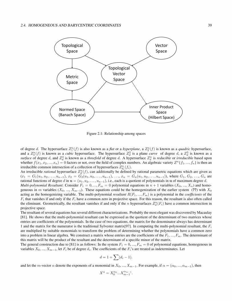
2.4. HOMOGENEOUS AND BARYCENTRIC COORDINATES 39
Topological Space
Metric Space
Normed Space (Banach Space)
Topological Vector Space
Vector Space
Inner Product Space
(Hilbert Space)
Figure 2.1: Relationship among spaces
of degree d. The hypersurface Zn1 (f) is also known as a flat or a hyperplane, a Zn2 (f) is known as a quadric hypersurface,and a Zn3 (f) is known as a cubic hypersurface. The hypersurface Z2
d is a plane curve of degree d, a Z3d is known as a
surface of degree d, and Z4d is known as a threefold of degree d. A hypersurface Znd is reducible or irreducible based upon
whether f(x1, x2, ..., xn) = 0 factors or not, over the field of complex numbers. An algebraic variety Znf1, ..., fn is then anirreducible common intersection of a collection of hypersurfaces Zndi(fi).An irreducible rational hypersurface Znd (f), can additionally be defined by rational parametric equations which are given as(x1 = G1(u1, u2, . . . , un−1), x2 = G2(u1, u2, . . . , un−1), . . ., xn = Gn(u1, u2, . . . , un−1)), where G1, G2, . . ., Gn arerational functions of degree d in u = (u1, u2, . . . , un−1), i.e., each is a quotient of polynomials in u of maximum degree d.Multi-polynomial Resultant: Consider F1 = 0, ..., Fm = 0 polynomial equations in n + 1 variables (X0, ..., Xn) and homo-geneous in m variables (X0, ..., Xm−1). These equations could be the homogenization of the earlier system (??) with X0
acting as the homogenizing variable. The multi-polynomial resultant R(F1, ..., Fm) is a polynomial in the coefficients of theFi that vanishes if and only if the Fi have a common zero in projective space. For this reason, the resultant is also often calledthe eliminant. Geometrically, the resultant vanishes if and only if the n hypersurfaces Znd (Fi) have a common intersection inprojective space.The resultant of several equations has several different characterizations. Probably the most elegant was discovered by Macaulay[81]. He shows that the multi-polynomial resultant can be expressed as the quotient of the determinant of two matrices whoseentries are coefficients of the polynomials. In the case of two equations, the matrix for the denominator always has determinant1 and the matrix for the numerator is the traditional Sylvester matrix[97]. In computing the multi-polynomial resultant, the Fiare multiplied by suitable monomials to transform the problem of determining whether the polynomials have a common zerointo a problem in linear algebra. We construct a matrix whose entries are the coefficients of the F1, ..., Fm. The determinant ofthis matrix will be the product of the resultant and the determinant of a specific minor of the matrix.The general construction due to [81] is as follows: In the system F1 = 0, ..., Fm = 0 of polynomial equations, homogenous invariables X0, ..., Xm−1, let Fi be of degree di. The coefficients of the Fi’s are treated as indeterminates. Let
d = 1 +∑
(di − 1).
and let the m-vector α denote the exponents of a monomial in X0, ..., Xm−1. For example, if α = (α0, ..., αm−1), then
Xα = Xα00 ...X
αm−1
m−1 .

40 CHAPTER 2. SETS, FUNCTIONS AND MAPPINGS
Thus, the set of all monomials of degree d in m variables is
X d = Xα|α0 + ...+ αm−1 = d.
If N denotes the number of monomials in this set, then the monomials will index the columns of an N by N matrix.
N =
(d+m− 1
d
)Partition X d into n disjoint sets. These sets are
X di = Xα|αi ≥ di and αj < dj ,∀j < i.
Next, for each set X di , construct a set F di of polynomials from Fi using monomials in X di . Specifically, let
F di =X dixdii
fi.
The F di are sets of homogeneous polynomials in m variables of degree d. Moreover, each of the polynomials in the union ofthe F di , equated to zero, collectively yields a set of N homogeneous polynomial equations. Construct an N by N matrix (callit A) whose columns are indexed by monomials in X d and whose rows correspond to the polynomials in the F di ’s. For a givenpolynomial P in F di , its row consists of the symbolic coefficients aik, bjk etc., of each monomial in P .
A
Xd
0
.
.
.Xdm−1
=
. ai1 ai2 ai3 . . . .. . bj1 bj2 bj3 . . .. . . . . . . .. . . . . . . .. . . . . . . .
Xd0
.
.
.Xdm−1
=
0...0
(2.2)
Now, if the Fi have a common root (X0, ..., Xm−1), then this root must satisfy all of the polynomial equations in the F di ’s.This fact implies that the nontrivial vector (X0, ..., Xm−1) must be in the null space of A. Thus, A must be singular orequivalently, the determinant of A (call it D) must be zero. This argument establishes that the resultant R is a factor of D. Theremaining factors of D are extraneous and have no bearing on whether the original equations have a common root. The beautyof Macaulay’s result is that he established that the extraneous factors are the determinant of a minor of A. This minor (call itB)can be constructed from A in the following manner. Delete all columns of A that correspond to monomials Xα where αi < difor all but one value of i. (Note there must at least one such i due to the manner in which d was chosen.) Delete all rows of Athat correspond to polynomials in Fi whose multipliers Xα have αj < dj for i < j ≤ n.Macaulay shows that the resultant R satisfies
R =det(A)
det(B)
where this division is carried out before the indeterminates forming the entries of A and B are specialized. The reason forspecializing after division is that det(A) and det(B) may evaluate to zero even though R is not identically zero. Techniquesfor computing R by specializing before division has recently been considered in [23, 92].Multi-polynomial Remainder Sequence: Consider first two polynomial equations f1(x1, . . . , xn) = 0 and f2(x1, . . . , xn) = 0.Treating them as polynomials in x1, the psuedo-remainder (f1/f2) = g(x1, . . . , xn) for degreex1 (f2) ≤ degreex1 (f1), is theresult of one step of psuedo-division in the ringC of coefficient polynomials in n−1 variables (x2, . . . , xn), i.e. αf1 = βf2−gwith α, βεC and degreex1
(g) < degreex1(f2). Repeating the psuedo-division with f2 and g and ensuring that the factors α and
β are ‘primitve’, one can compute a subresultant polynomial remainder sequence (p.r.s):
f1, f2, g = Sk−1, . . . , S1, S0 (2.3)
where Si is the psuedo-remainder of the two polynomials preceding it in the sequence and is known as the ith subresultant off1 and f2, with respect to x1, see for e.g [66, 80]. Here S0 is a polynomial independent of x1 and is the resultant of f1 and f2,with respect to x1. (Note in the homogeneous case S0 is the polynomial resultant of F1 and F2, with respect to X0 and X1.

2.4. HOMOGENEOUS AND BARYCENTRIC COORDINATES 41
For the set of polynomial equations ( ??), treating them as polynomials in x1, we select the polynomial, say fk, of minimumdegree in x1. We then compute the subresultant psuedo-remainder for each pair (fi/fk) = gi, 1 ≤ i ≤ m and i 6= k, yielding anew system of equations gi and fk. We repeat the above, first selecting from the new system, a polynomial of minimum degreein x1, and then computing pairwise subresultant psuedo-remainders. Eventually, we obtain a system of m − 1 polynomialequations, say Sm−1
f1(x2, ..., xn) = 0
...
fm−1(x2, ..., xn) = 0 (2.4)
independent of x1.The above is then one (macro) step of the multi-equational polynomial remainder sequence (m.p.r.s). For the new set ofpolynomial equations (2.4), treating them as polynomials in x2, we repeat the entire process above and obtain yet anotherreduced system Sm−2 of m − 2 polynomial equations, all independent of x2, and so on. This sequence of systems of multi-equational polynomial equations
S = Sm, Sm−1, Sm−2, . . . , S1, S0 (2.5)
is what we term the multi-equational polynomial remainder sequence.
2.4.2 Barycentric coordinatesBarycentric coordinates are a natural method for describing a function defined on a triangular domain and we can extend theidea of barycentric coordinates over polygon or in higher dimensional simplex. Barycentric coordinates on general polygons(denotes as generalized barycentric coordinates) are any set of functions satisfying certain key properties.
Definition 2.27. Functions λi : Ω→ R, i = 1, . . . , n are barycentric coordinates on Ω if they satisfy two properties.
B1. Non-negative: λi ≥ 0 on Ω.
B2. Linear Completeness: For any linear function L : Ω→ R, L =
n∑i=1
L(vi)λi.
Most commonly used barycentric coordinates, including the mean value coordinates, are invariant under rigid transformationand simple scaling which we will state precisely. Let T : R2 → R2 be a composition of rotation, translation, and uniformscaling transformations and let λTi denote a set of barycentric coordinates on TΩ.
B3. Invariance: λi(x) = λTi (T (x)).
The invariance property can be easily passed through Sobolev norms and semi-norms, allowing attention to be restricted todomains Ω with diameter one without loss of generality. The essential case in our analysis is the H1-norm, |u|H1(Ω) =√∫|∇u(x)|2 dx where∇u = (∂u/∂x, ∂u/∂y)T is the vector of first partial derivatives of u, and for simplicity T is a uniform
transformation, T (x) := hx. For simplicity , the Euclidean norm of vectors will be denoted with single bars |·| without anysubscript. Applying the chain rule and change of variables in the integral gives the equality:
∣∣λTi ∣∣2H1(TΩ)=
∫TΩ
∣∣∇λTi (x)∣∣2 dx =
∫TΩ
∣∣∣∣ 1h∇ (λTi (hx))∣∣∣∣2 dx
= hd−2
∫Ω
|∇λi(y)|2 dy = hd−2 |λi|2H1(Ω) .
The scaling factor hd resulting from the Jacobian when changing variables in the integral is the same for any Sobolev seminorm,while the factor of h−2 from the chain rule depends on the order of differentiation in the norm (1, in this case) and the Lp semi-norm used (p = 2, in this case). When developing interpolation error estimates, which are ratios of Sobolev norms, the formerterm (i.e., the chain of variables portion) cancels out and latter term (i.e., the chain rule portion) determines the convergencerate.Several other familiar properties immediately result from the definition of generalized barycentric coordinates (B1 and B2).

42 CHAPTER 2. SETS, FUNCTIONS AND MAPPINGS
B4. Partition of unity:n∑i=1
λi ≡ 1.
B5. Linear precision:n∑i=1
viλi(x) = x.
B6. Interpolation: λi(vj) = δij .
Proposition 2.28. Suppose B1 and B2 hold. Then B4, B5, and B6 hold as well.
Example: Triangulation Barycentric Coordinates
We begin with the simplest possible case of describing a line passing through a triangle. Let T be a triangle with vertices(x1, y1), (x2, y2), (x3, y3). To represent a line C implicitly, we could find real coefficients cij ∈ R of a function
g(x, y) =∑i+j≤1
cijxiyj = c00 + c10x+ c01y
such that C = g = 0. Since the function g is defined in terms of the global coordinates x and y, it is not immediately obviousgiven the coefficients cij whether C passes through T at all. Thus, we transform the (x, y) coordinates to real barycentriccoordinates (λ1, λ2, λ3) via x
y1
=
x1 x2 x3
y1 y2 y3
1 1 1
λ1
λ2
λ3
Under the mapping, (x1, y1) becomes (1, 0, 0), (x2, y2) becomes (0, 1, 0), and (x3, y3) becomes (0, 0, 1). We can now seekreal coefficients γi ∈ R of a function
g(λ1, λ2, λ3) =
3∑i=1
γiλi
such that C = g = 0. The coefficients are very easily described: γi is the value of g at (xi, yi). Accordingly, if at least oneγi is positive and at least one is negative, C will pass through T , intersecting at the edges between vertices with opposite signs.Thus, barycentric coordinates give us an easy way to define and control the shape of lines through a triangle.To describe more complicated curves through T , we use a generalization of barycentric coordinates. Fix a degree n ≥ 1 andcompute the trinomial expansion of
(λ1 + λ2 + λ3)d
= 1.
This will yield(d+2
2
)terms of the form λi1λ
j2λk3 with i+ j + k = n. These functions, called the Bernstein polynomials, form
a basis for degree n polynomials in R2 and can be used analogously to the linear case.(Which will be covered later) In standardcoordinates, we could find real coefficients cij ∈ R
g(x, y) =∑i+j≤n
cijxiyj
such that C = g = 0. This problem is much more difficult than the linear case, making the barycentric coordinate changeessential. We seek instead the real Bernstein-Bézier coefficients γijk ∈ R of the function
g(λ1, λ2, λ3) =∑
i+j+k=n
γijkd!
i!j!k!λi1λ
j2λk3 (2.6)
such that C = g = 0. As with barycentric coordinates, the coefficient at a vertex of the triangle is exactly the value of g atthe vertex, for example
γ300 = g(1, 0, 0) = g(x1, y1).
The remaining coefficients control the properties of g (and hence its level sets) within T . The coefficients are associated to thedomain points on a regular subdivision of the triangle. We show examples of such subdivisions for n = 2 and n = 3 in Figure2.2.Besides triangulation coordinates, there are several other type of coordinates that we would like to introduce:

2.5. POLYNOMIALS, PIECEWISE POLYNOMIALS, SPLINES 43
Figure 2.2: Domain points associated to Bernstein-Bézier coefficients for n = 2 (left) and n = 3 (right).
Harmonic Coordinates
Mean Value Coordinates
Wachspress Coordinate
2.5 Polynomials, Piecewise Polynomials, SplinesIn this section, we will bring examples of basis from functional space that can be used to interpret geometric objects (in practice,i.e. are lines and surfaces). The bases are first defined for restricted subdomains of the defining space as opposed to the powerbasis which is defined for all points of the space. They are mostly compacted supported, not infinitively supported, but theyhave better properties other than simplest power basis. The example formulations given below are defined for values of each ofthe variables x, y and z in the unit interval [0,1]. We will introduce each the following.
2.5.1 Univariate caseBernstein-Bezier
P (x) =
m∑j=0
wjBmj (x)
where
Bmi (x) =
(m
i
)xi(1− x)m−i
B-Spline
The B-spline basis over the unit interval [0,1] is easily generated by a fractional linear recurrence as given below for the uni-variate case. The bivariate and trivariate forms can also be similarly generated from this in either tensor product or barycentricform. (See examples in BB form)The univariate B-spline form is defined by linear combination of control points plnl=0 :
Pn =
m∑l=0
plNnl (x)
where Nnl (x) is defined via knot sequence 0 = u0 ≤ u1 < . . . < um+1 = 1 :
N1l (x) =
1 for ul ≤ ul+1
0 otherwise.

44 CHAPTER 2. SETS, FUNCTIONS AND MAPPINGS
Nnl (x) =
x− ul−1
ul+n−1 − ul−1Nn−1l (x) +
ul+n − xul+n − ul
Nn−1l+1 (x)
2.5.2 Bivariate case
Tensor Product
P (x, y) =
m∑i=0
n∑j=0
wijBni (x)Bnj (y)
Generalized Barycentric Coordinate on convex Polygon
P (x, y) =
m∑i=0
m−i∑j=0
wijBnij(x, y)
where
Bmij (x, y) =
(m
ij
)xiyj(1− x− y)m−i−j
Here (x, y)→ (x, y, 1− x− y) is a naive mapping from world coordinate to the barycentric coordinate.
2.5.3 Multivariate case
Tensor Product
p(x1, . . . , xd) =
n1∑i1=0
. . .
nd∑id=0
bi1i2...id Bn1i1
(t1)Bn2i2
(t2) . . . Bndid
(td) (2.7)
where
(x1, . . . , xd)T ∈ [a1, b1]× [a2, b2]× . . .× [ad, bd]
ti = xi−aibi−ai , i = 1, 2, . . . , d
Bni (t) = n!i!(n−i)! t
i(1− t)n−i
Generalized Barycentric Coordinate on Simplex
P (x, y, z) =
m∑i=0
m−i∑j=0
m−i−j∑k=0
wijkBmijk(x, y, z)
where
Bmijk(x, y, z) =
(m
ijk
)xiyjzk(1− x− y − z)m−i−j−k
Mixed Bernstein Form
Take the simplest tetrahedron as the example:
P (x, y, z) =
m∑i=0
m−i∑j=0
p∑k=0
bijkBnij(x, y)Bnk (z)

2.6. PARAMETRIC AND IMPLICIT REPRESENTATION 45
Let d = d1 + d2, p0, . . . ,pd1 ∈ Rd1 be affine independent. Then the mixed Bernstein form is
p(x1, . . . , xd) =∑
i1+...+id1≤m
n1∑j1=0
. . .
nd2∑jd2=0
bi1...id1 j1...jd2 Bmi1...id1
(α1, . . . , αd1) Bn2j1
(t1) . . . Bnd2jd2
(td2) (2.8)
where(x1, . . . xd)
T ∈ [p0, . . . ,pd1 ]× [a1, b1]× . . .× [ad2 , bd2 ]x1
...xd11
=
[p0 p1 . . . pd11 1 . . . 1
] α0
α1
...αd1
and
ti =xd1+i − ai
bi − ai i = 1, 2, . . . , d2
If d1 = 0, then p is the Bernstein form on hypercube. If d2 = 0, then p is the Bernstein form on simplex.
2.6 Parametric and Implicit RepresentationWe will continue discuss two different representation based on definition and notation in 2.4 and 2.5.3 : what is parametric andwhat is implicit? How will they represent 2d and 3d objects (or in higher degree)? And how they are different from.For notation simplicity, all function fi , no matter univariate,bivariate or multivariate, will be generalized as the linear combi-nation we proposed in 2.5.3.
2.6.1 CurvesA real implicit algebraic plane curve f(x, y) = 0 is a hypersurface of dimension 1 in R2, while a parametric plane curve[f3(s)x − f1(s) = 0, f3(s)y − f2(s) = 0] is an algebraic variety of dimension 1 in R3, defined by the two independentalgebraic equations in the three variables x, y, s.A plane parametric curve is a very special algebraic variety of dimension 1 in x, y, s space, since the curve lies in the 2-dimensional subspace defined by x, y and furthermore points on the curve can be put in (1, 1) rational correspondence withpoints on the 1-dimensional sub-space defined by s. Parametric curves are thus a special subset of algebraic curves, andare often also called rational algebraic curves. Figure 2.3 depicts the relationship between the set of parametric curves andnon-parametric curves at various degrees.Example parametric (rational algebraic) curves are degree two algebraic curves (conics) and degree three algebraic curves(cubics) with a singular point. The non-singular cubics are not rational and are also known as elliptic cubics. In general, anecessary and sufficient condition for the rationality of an algebraic curve of arbitrary degree is given by the Cayley-Riemanncriterion: a curve is rational if and only if g = 0, where g, the genus of the curve is a measure of the deficiency of thecurve’s singularities from its maximum allowable limit [112]. Algorithms for computing the genus of an algebraic curve andfor symbolically deriving the parametric equations of genus 0 curves, are given for example in [1].For implicit algebraic plane curves and surfaces defined by polynomials of degree d, the maximum number of intersectionsbetween the curve and a line in the plane or the surface and a line in space, is equal to the maximum number of roots ofa polynomial of degree d. Hence, here the geometric degree is the same as the algebraic degree which is equal to d. Forparametric curves defined by polynomials of degree d, the maximum number of intersections between the curve and a line inthe plane is also equal to the maximum number of roots of a polynomial of degree d. Hence here again the geometric degree isthe same as the algebraic degree.For parametric surfaces defined by polynomials of degree d the geometric degree can be as large as d2, the square of thealgebraic degree d. This can be seen as follows. Consider the intersection of a generic line in space [a1x + b1y + c1z − d1 =0, a2x + b2y + c2z − d2 = 0] with the parametric surface. The intersection yields two implicit algebraic curves of degree dwhich intersect in O(d2) points (via Bezout’s theorem), corresponding to the intersection points of the line and the parametricsurface.

46 CHAPTER 2. SETS, FUNCTIONS AND MAPPINGS
Implicit Quartics
Planar Implicit and Parametrics
Implicit Degree Eight
Implicit Degree Nine
Implicit Cubics
GEOMETRIC
DEGREE
1
2
3
4
8
9
Quadratic Implicit and Parametrics
Curves
Curves
Degree Nine Parametrics
Degree Eight Parametrics
Quartic
Parametrics
Cubic
Parametrics
SeparatingParametric andNon-parametricCurves
ParametricsQuadratic
Implicit Quartics
Planar Implicit and Parametrics
Cubic Parametrics
Biquadratic Parametrics
Implicit Degree Eight Surfaces
Implicit Degree Nine Surfaces
Implicit Cubics
Implicit Quadrics
GEOMETRIC
DEGREE
1
2
3
4
8
9
SeparatingParametric &Non-parametricSurfaces
Figure 2.3: A classification of low degree algebraic curves (left) and surfaces (right)
2.6. PARAMETRIC AND IMPLICIT REPRESENTATION 47
A parametric curve of algebraic degree d is an algebraic curve of genus 0 and so have (d−1)(d−2)2 = O(d2) singular (double)
points. This number is the maximum number of singular points an algebraic curve of degree d may have. From Bezout’stheorem, we realize that the intersection of two implicit surfaces of algebraic degree d can be a curve of geometric degreeO(d2). Furthermore the same theorem implies that the intersection of two parametric surfaces of algebraic degree d (andgeometric degree O(d2)) can be a curve of geometric degree O(d4). Hence, while the potential singularities of the space curvedefined by the intersection of two implicit surfaces defined by polynomials of degree d can be as many as O(d4), the potentialsingularities of the space curve defined by the intersection of two parametric surfaces defined by polynomials of degree d canbe as many as O(d8).Let C : (f1(x, y, z) = 0, f2(x, y, z) = 0) implicitly define an irreducible algebraic space curve of degree d. The irreducibilityof the curve is not really a restriction, since reducible curves can be handled similarly by treating each irreducible componentin turn. The situation is slightly more complicated if in the real setting, we may wish to achieve separate containment of eachreal component of an irreducible curve. We defer a solution to this problem, and for the time being consider it reduced to theproblem of choosing appropriate clipping surfaces to isolate that real component, after the interpolated surface is computed.Note for parametrically defined curves, this problem does not arise.
2.6.2 SurfaceSimilarly, a real implicit algebraic surface f(x, y, z) = 0 is a hypersurface of dimension two in R3, while a parametric surface[f4(s, t)x−f1(s, t) = 0, f4(s, t)y−f2(s, t) = 0, f4(s, t)z−f3(s, t) = 0] is an algebraic variety of dimension 2 in R5, definedby three independent algebraic equations in the five variables x, y, z, s, t.When a curve is given in rational parametric form, its equations can be used directly to produce a linear system for interpolation,instead of first computing nd+ 1 points on the curve. Let C : (x = G1(t), y = G2(t), z = G3(t)) be a rational curve of degreed. An interpolating surface S : f(x, y, z) = 0 of degree n which contains C is computed as follows:
B1. Substitute (x = G1(t), y = G2(t), z = G3(t)) into the equation f(x, y, z) = 0.
B2. Simplify and rationalize to obtain Q(t) = 0, where Q is a polynomial in t, of degree at most nd, and with coefficientswhich are linear expressions in the coefficients of f . For Q to be identically zero, each of its coefficents must be zero,and hence we obtain a system of at most nd + 1 linear equations, where the unknowns are the coefficients of f . Anynon-trivial solution of this linear system will represent a surface S which interpolates C.
The proof of correctness of the algorithm follows from the lemma below.
Lemma 2.29. The containment condition is satisfied by step 2. of the above algorithm
Proof: We omit this here and refer the reader to the full paper.
Parametric Curves
Parametric Surface
2.6.3 ExamplesConics
The general conic implicit equation is given by
C(x, y) = ax2 + by2 + cxy + dx+ ey + f = 0.
The non-trivial case in converting this to a rational parameterization arises when a and b are both non-zero. Otherwise onealready has one variable ( x, or y) in linear form and expressible as a rational polynomial expression of the other, and hencea rational parameterization. This then suggests that to obtain a rational parameterization all we need to do is to make C(x, y)non-regular in x or y. That is, eliminate the x2 or the y2 term through a coordinate transformation. For then one of the variablesis again in linear form and is expressible as a rational polynomial expression of the other. We choose to eliminate the y2 term,by an appropriate coordinate transformation applied to C(x, y). This is always possible and the algorithm is now describedbelow. (The entire algorithm which also handles all trivial and degenerate cases of the conic is implemented on a VAX-780using VAXIMA.)

48 CHAPTER 2. SETS, FUNCTIONS AND MAPPINGS
Geometrically speaking, a conic being irregular in x or y means that most lines parallel to the x or y axis respectively, intersectthe curve in one point. Also, most lines through a point (b1, b2) on the conic meet the conic in one additional point. By sendingthis point ( b1, b2) to infinity we make all these lines parallel to some axis and the curve irregular in one of the variables ( x, or y)and hence amenable to parameterization. The coordinate transformation we select is thus one which sends the point ( b1, b2) onthe conic to infinity. The rational parameterization we obtain is global, of degree at most 2 and with parameter t correspondingto the slopes of the lines through the point (b1, b2) on the conic. Further t ranges from (−∞,∞) and covers the entire curve.The selection of the point ( b1, b2) on the conic becomes important and may be made appropriately, when the parameterizationis desired only for a specific piece of the conic.
Step (1) IfC(x, y) has a real root at infinity, a linear transformation of the type x′ = a1x + b1y + c1 and y′ = a2x + b2y + c2will suffice. If C(x, y) has no real root at infinity, we must use a linear transformation of the type x′ = ( a1x + b1y + c1)/(a3x + b3y + c3) and y′ = a2x + b2y + c2)/( a3x + b3y + c3). This is equivalent to a homogeneous linear transformationof the type X ′ = a1X + b1Y + c1H , Y ′ = a2X + b2Y + c2H and H ′ = a3X + b3Y + c3H applied to the homogeneousconic C(X,Y,H) = aX2 + bY 2 + cXY + dXH + eY H + fH2 = 0.
Step (2) Points at infinity for C(x, y) are given by the linear factors of the degree form (highest degree terms) of I . For theconic this corresponds to a real root at infinity if c2 >= 4ab, (e.g. parabolas and hyperbolas). For otherwise both roots atinfinity are complex , (complex roots arise in conjugate pairs). Further for c2 = 4ab, (e.g. parabolas), the degree form is aperfect square and this gives a polynomial parameterization for the curve.
Step (3) Applying a linear transformation for c2 >= 4ab, gives rise to C(x′, y′) = I( a1x + b1y + c1, a2x + b2y + c2).To eliminate the y2 term we need to choose b1 and b2 such that ab21 + cb1b2 + bb22 = 0. Here both the values of b1 and b2can always be chosen to be real.
Step (4) Applying a homogeneous linear transformation for c2 < 4ab, gives rise toC(X ′, Y ′, H ′) =C(a1X + b1Y + c1H ,a2X + b2Y + c2H , a3X + b3Y + c3H). To eliminate the Y 2 term we need to choose b1, b2 and b3 such that ab21 + bb22 +cb1b2 + db1b3 + eb2b3 + fb23 = 0. This is equivalent to finding a point ( b1, b2, b3) on the homogeneous conic. The values of b1and b2 are both real if (cd− 2ae) is not less than the geometric mean of 4af − d2 and 4ab − c2, or alternatively (ce− 2bd)is not less than the geometric mean of 4bf − e2 and 4ab − c2.
Step (5) Finally choose the remaining coefficients ai’ s, ci’ s, ensuring that the appropriate transformation is well defined. Inthe case of a linear transformation, this corresponds to ensuring that the matrix(
a1 b1a2 b2
)is non-singular. Hence ci’ s can be chosen to be 0 and a1 = 1, a2 = 0. In the case of a homogeneous linear transformation, oneneeds to ensure that the matrix a1 b1 c1
a2 b2 c2a3 b3 c3
is non-singular. Here a1 = 1, c2 = 1 and the rest set to 0 suffices. These remaining coefficients provide a measure of local controlfor the curve and may also be chosen in a way that gives specific local parameterizations for pieces of the curve, appropriatefor particular applications.
Conicoids
The case of the conicoid is a generalization of the method of the conic. The general conicoid implicit equation is given byC(x, y, z) = ax2 + by2 + cz2 + dxy + exz + fyz + gx + hy + iz + j = 0. Again the main case of concern is when a, b and c areall non-zero. Otherwise one already has one of the variables ( x, y, or z) in linear form and expressible as a rational polynomialexpression of the other two. This then suggests that to obtain the rational parameterization all we need to do again is to makeC(x, y, z) non-regular in say, y. That is, eliminate the y2 term through a coordinate transformation. For then y is in linear form

2.6. PARAMETRIC AND IMPLICIT REPRESENTATION 49
and is expressible as a rational polynomial expression of the other two. We eliminate the y2 term by an appropriate coordinatetransformation applied to C(x, y, z). This is always possible and the algorithm is now described below. (The entire algorithmwhich also handles all trivial and degenerate cases of the conicoid is implemented on a VAX-780 using VAXIMA. )Geometrically speaking, a conicoid being irregular in x, y or z means that most lines parallel to the x, y or z axis respectively,intersect the surface in one point. Also, most lines through a point (b1, b2, b3) on the conicoid meet the conicoid in one additionalpoint. By sending this point ( b1, b2, b3) to infinity we make all these lines parallel to some axis and the surface irregular in oneof the variables ( x, or y) and hence amenable to parameterization. The coordinate transformation we select is thus one whichsends the point ( b1, b2, b3) on the conicoid to infinity. The rational parameterization we obtain is global, of degree at most 2and with parameters s and t corresponding to the ratio of the direction cosines of the lines through the point (b1, b2, b3) on theconicoid. Further s and t both range from (−∞,∞) and cover the entire surface. The selection of the point ( b1, b2, b3) on theconicoid becomes important and may be made appropriately, when the parameterization is desired only for a specific patch ofthe conicoid.
Step (1) If C(x, y, z) has a real root at infinity, alinear transformation of the type x′ = a1x + b1y + c1z + d1, y′ =a2x + b2y + c2z + d2 and z′ = a3x + b3y + c3z + d3 will suffice. If C(x, y, z) has no real root at infinity, we must use alinear transformation of the type x′ = ( a1x + b1y + c1z + d1)/( a4x + b4y + c4z + d4), y′ = a2x + b2y + c2z + d2)/(a4x + b4y + c4z + d4). and z′ = ( a3x + b3y + c3z + d3)/( a4x + b4y + c4z + d4). This is equivalent to ahomogeneous linear transformation of the type X ′ = a1X + b1Y + c1Z + d1H , Y ′ = a2X + b2Y + c2Z + d2H , Z ′ =a3X + b3Y + c3Z + d3H and H ′ = a4X + b4Y + c4Z + d4H applied to the homogeneous conicoid C(X,Y, Z,H) =aX2 + bY 2 + cZ2 + dXY + eXZ + fY Z + gXH + hY H + iZH + jH2 = 0,
Step (2) Points at infinity for C(x, y) are given by the linear factors of the degree form (highest degree terms) of I . For theconicoid this corresponds to the roots of the homogeneous conic equation C(x, y, z) = ax2 + by2 + dxy + exz + fyz + cz2 =0. Also, here the simultaneous truth of d2 = 4ab, e2 = 4ac and f2 = 4bc corresponds to the existence of a polynomialparameterization for the conicoid, as then the degree form is a perfect square.
Step (3) Apply a linear transformation if a real root (rx, ry, rz) exists for the homogeneous conic C(x, y, z) of (2). This givesrise to C(x′, y′, z′) = I( a1x + b1y + c1z + d1, a2x + b2y + c2z + d2, a3x + b3y + c3z + d3). To eliminate the y2
term we can take ( b1, b2, b3) = ( rx, ry, rz), the real point on C(x, y, z).
Step (4) Apply a homogeneous linear transformation if only complex roots exist for the homogeneous conic C(x, y, z) of (2).This gives rise toC(X ′, Y ′, Z ′, H ′) = I( a1X + b1Y + c1Z + d1H , a2X + b2Y + c2Z + d2H , a3X + b3Y + c3Z + d3H ,a4X + b4Y + c4Z + d4H). To eliminate the Y 2 term we choose b4 = 1 and ( b1, b2) to be a point on either the conic ax2 +by2 + dxy + gxz + hyz + jz2 = 0 with b3 = 0 or a point on the conic ax2 + by2 + dxy + (e+ g)xz + (f + h)yz + (c+ i+ j)z2
= 0 with b3 = 1. Real values exist for b1 and b2 if there exists a real point on either of the above conics.
Step (5) Finally choose the remaining coefficients ai’ s, ci’ s, and di’ s, ensuring that the appropriate transformation is welldefined. In the case of a linear transformation, this corresponds to ensuring that the matrix a1 b1 c1
a2 b2 c2a3 b3 c3
is non-singular. Here the di’ s can be chosen to be 0. Further a2 = 1, c3 = 1 if b1 is non-zero or else a1 = 1, c3 = 1 if b2 isnon-zero or else a1 = 1, c2 = 1, with the rest set to 0. In the case of a homogeneous linear transformation one needs to ensurethat the matrix
a1 b1 c1 d1
a2 b2 c2 d2
a3 b3 c3 d3
a4 b4 c4 d4

50 CHAPTER 2. SETS, FUNCTIONS AND MAPPINGS
is non-singular. Here a1 = 1, c3 = 1, d2 = 1 with the rest set to 0 suffices. These remaining coefficients provide a measureof local control for the surface and may also be chosen in a way that gives specific local parameterizations for pieces of thesurface, appropriate for particular applications.
2.7 Finite Elements and Error Estimation
2.7.1 Tensor Product Over The Domain: Irregular Triangular Prism
Definition
Given the triangulation mesh T , let [vivjvk] be one of the triangles where vi, vj , vk are the vertices of the triangle. Supposethe unit normals of the surface at the vertices are also known, denoted as nl, (l = i, j, k). Let vl(λ) = vl + λnl. First wedefine a prism (Figure 2.4) Dijk := p : p = b1vi(λ) + b2vj(λ) + b3vk(λ), λ ∈ Iijk, where (b1, b2, b3) are the barycentriccoordinates of points in [vivjvk], and Iijk is a maximal open interval containing 0 and for any λ ∈ Iijk, vi(λ), vj(λ), vk(λ)are not collinear and ni, nj , nk point to the same side of the plane Pijk(λ) := p : p = b1vi(λ) + b2vj(λ) + b3vk(λ). Next
Figure 2.4: A prism Dijk constructed based on the triangle [vivjvk].
we define a function in the Bernstein-Bezier (BB) basis over the prism Dijk:
F (b1, b2, b3, λ) =∑
i+j+k=n
bijk(λ)Bnijk(b1, b2, b3), (2.9)
where Bnijk(b1, b2, b3) is the Bezier basis
Bnijk(b1, b2, b3) =n!
i!j!k!bi1b
j2bk3 .
Figure 2.5: The control coefficients of the cubic Bezier basis of function F .

2.7. FINITE ELEMENTS AND ERROR ESTIMATION 51
Non-degenerancy
(yiwang) : I am not sure if the subsection title is correct Let p(l)ijk(λ) = det[nl, vj(λ) − vi(λ), vk(λ) −vi(λ)], l = i, j, k.
Assumep
(l)ijk(λ) > 0, ∀λ ∈ [0, 1], l = i, j, k . (2.10)
Consider the real numbers λ1, · · · , λs (s ≤ 6) that solve one of these three equations of degree 2: p(l)ijk(λ) = 0, l = i, j, k,
and define a = max(−∞, λl : λl < 0), b = min(+∞, λl : λl > 1), and Iijk = (a, b). Then Iijk is the largest intervalcontaining [0, 1] such that Pijk(Iijk) is non-degenerate. To show this fact, note that a triangle Tijk(λ) is non-degenerate if andonly if
nTl [vj(λ)− vi(λ)]× [vk(λ)− vi(λ)] = p(l)ijk(λ) > 0, (2.11)
l = i, j, k, where× denotes the cross product of two vectors. The assumption ((2.10)) implies that [0, 1] ⊂ I . Since p(l)ijk(0) > 0
and p(l)ijk(1) > 0, for l = i, j, k, then p(l)
ijk(λ) > 0 for λ ∈ (a, b) and l = i, j, k. Since p(l)ijk(a) = 0 for l = i or l = j or l = k if
a > −∞, a is the infimum of the interval of λ that contains [0, 1] and makes (2.11) hold. Similarly, b is the supremum of suchan interval. Therefore Iijk is the largest interval such that Pijk(Iijk) is non-degenerate.
Smoothness
We can then approximate the given surface by the zero contour of F , denoted as S. In order to make S smooth, the degree ofthe Bezier basis n should be no less than 3. For simplicity, here we consider the case of n = 3. The control coefficients bijk(λ)should be properly defined such that S is continuous. In Figure 2.5 we show the relationship of the control coefficients and thepoints of the triangle when n = 3. Next we are going to discuss these coefficients are defined.Since S passes through the vertices vi, vj , vk, we define
b300 = b030 = b003 = λ. (2.12)
Next we are going to define the coefficients on the edges of the triangle in Figure 2.5. To obtain C1 continuity at vi, werequire that the directional derivatives of F at vi in the direction of b2 and b3 are equal to∇F · (vj − vi) and∇F · (vk − vi),respectively. Noticing that F has the form of (2.9) and (b1, b2, b3) = (1, 0, 0) at vi, one can derive that b210 − b300 =13∇F (vi) · (vj(λ)− vi(λ)), where∇F (vi) = ni. Therefore
b210 = λ+1
3ni · (vj(λ)− vi(λ)). (2.13)
b120, b201, b102, b021, b012 are defined similarly.To obtain the C1 continuity at the midpoints of the edges of T , we define b111 by using the side-vertex scheme [?]:
b111 = w1b(1)111 + w2b
(2)111 + w3b
(3)111, (2.14)
where
wi =b2jb
2k
b22b23 + b21b
23 + b21b
22
, i = 1, 2, 3, i 6= j 6= k.
Next we are going to define b(1)111, b(2)
111 and b(3)111. In Appendix ?? we prove that our scheme of defining this three coefficients
can guarantee the C1 continuity at the midpoints of the edges vjvk, vivk and vivj . Consider the edge vivj . Recall that anypoint p = (x, y, z) in Dijk can be represented by
(x, y, z)T = b1vi(λ) + b2vj(λ) + b3vk(λ). (2.15)
Therefore differentiating both sides of (2.15) with respect to x, y and z, respectively, yields
I3 =
∂b1∂x
∂b2∂x
∂λ∂x
∂b1∂y
∂b2∂y
∂λ∂y
∂b1∂z
∂b2∂z
∂λ∂z
(vi(λ)− vk(λ))T
(vj(λ)− vk(λ))T
(b1ni + b2nj + b3nk)T
, (2.16)

52 CHAPTER 2. SETS, FUNCTIONS AND MAPPINGS
where I3 is a 3× 3 unit matrix. Denote
M :=
(vi(λ)− vk(λ))T
(vj(λ)− vk(λ))T
(b1ni + b2nj + b3nk)T
, (2.17)
and let A = vi(λ)− vk(λ), B = vj(λ)− vk(λ) and C = b1ni + b2nj + b3nk, then M = (A B C)T. From (2.16) we have ∂b1∂x
∂b2∂x
∂λ∂x
∂b1∂y
∂b2∂y
∂λ∂y
∂b1∂z
∂b2∂z
∂λ∂z
= M−1 =1
det(M)(B × C, C ×A, A×B) . (2.18)
According to (2.9), at the midpoint of vivj , (b1, b2, b3) = (12 ,
12 , 0), we have ∂F
∂b1∂F∂b2∂F∂λ
=
(vi(λ)− vk(λ))T
(vj(λ)− vk(λ))T
(ni + nj)T/2
(ni + nj4
)+
32 (b210 − b111)32 (b120 − b111)
12
.
By (2.14), at (b1, b2, b3) = (12 ,
12 , 0) we have b111 = b
(3)111. Therefore the gradient at ( 1
2 ,12 , 0) is
∇F = M−1(∂F
∂b1,∂F
∂b2,∂F
∂λ)T
=ni + nj
4+
1
2 det(M)[3(b210 − b(3)
111)B × C + 3(b120 − b(3)111)C ×A+A×B] (2.19)
Define vectors
d1(λ) = vj(λ)− vi(λ) = B −A,d2(b1, b2, b3) = b1ni + b2nj + b3nk = C,
d3(b1, b2, b3, λ) = d1 × d2 = B × C + C ×A. (2.20)
Let
c = C(1
2,
1
2, 0), (2.21)
d3(λ) = d3(1
2,
1
2, 0, λ) = B × c + c×A. (2.22)
Let ∇F = ∇F ( 12 ,
12 , 0). In order to have C1 continuity at ( 1
2 ,12 , 0), we should have ∇F · d3(λ) = 0. Therefore, by (2.19)
and (2.22), we have
b(3)111 =
d3(λ)T(3b210B × c + 3b120c×A+A×B)
3‖d3(λ)‖2 . (2.23)
Similarly, we may define b(1)111 and b(2)
111.Now the function F (b1, b2, b3, λ) is well defined. The next step is to extract the zero level set S. Given the barycentric coordi-nates (b1, b2, b3) of a point in the triangle [vivjvk], we find the corresponding λ by solving the equation F (b1, b2, b3, λ) = 0for λ and this could be done by the Newton’s method. Then we may get the corresponding point on S as
(x, y, z)T = b1vi(λ) + b2vj(λ) + b3vk(λ). (2.24)
We have the following property for surface S:
Theorem 2.7.1. S is C1 at the vertices of T and the midpoints of the edges of T .Theorem 2.7.2. S is C1 everywhere if every edge vivj of T satisfies ni · (vi − vj) = nj · (vj − vi).Theorem 2.7.3. S is C1 everywhere if the unit normals at the vertices of T are the same.
Proofs of the theorems are shown in the [124].

2.8. BIOLOGICAL APPLICATIONS 53
2.7.2 Error Estimation
We consider first-order interpolation operators from some generalization of barycentric coordinates to arbitrary convex poly-gons. A set of barycentric coordinates λi for Ω associated with the interpolation operator I : H2(Ω)→ spanλi ⊂ H1(Ω)is given by
Iu :=∑i
u(vi)λi. (2.25)
Since barycentric coordinates are unique on triangles, this is merely the standard linear Lagrange interpolation operator whenΩ is a triangle.Before stating any error estimates, we fix some notation. For multi-index α = (α1, α2) and point x = (x, y), define xα :=xα1yα2 , α! := α1α2, |α| := α1 + α2, and Dαu := ∂|α|u/∂xα1∂yα2 . The Sobolev semi-norms and norms over an open set Ωare defined by
|u|2Hm(Ω) :=
∫Ω
∑|α|=m
|Dαu(x)|2∂x and ||u||2Hm(Ω) :=∑
0≤k≤m
|u|2Hm(Ω) .
The H0-norm is the L2-norm and will be denoted ||·||L2(Ω).Analysis of the finite element method often yields bounds on the solution error in terms of the best possible approximation inthe finite-dimensional solution space. Thus the challenge of bounding the solution error is reduced to a problem of finding agood interpolant. In many cases Lagrange interpolation can provide a suitable estimate which is asymptotically optimal. Forfirst-order interpolants that we consider, this optimal convergence estimate has the form
||u− Iu||H1(Ω) ≤ C diam(Ω) |u|H2(Ω) , ∀u ∈ H2(Ω). (2.26)
To prove estimate (2.26) in our setting, it is sufficient to restrict the analysis to a class of domains with diameter one and showthat I is a bounded operator from H2(Ω) into H1(Ω), that is
||Iu||H1(Ω) ≤ CI ||u||H2(Ω) , ∀u ∈ H1(Ω). (2.27)
We call equation (2.27) the H1 interpolant estimate associated to the barycentric coordinates λi used to define I .The optimal convergence estimate (2.26) does not hold uniformly over all possible domains; a suitable geometric restrictionmust be selected to produce a uniform bound. Even in the simplest case (Lagrange interpolation on triangles), there is a gapbetween geometric criteria which are simple to analyze (e.g. the minimum angle condition) and those that encompass the largestpossible set of domains (e.g. the maximum angle condition).
Geometric Criteria
TBD
2.8 Biological Applications
Complementary space visualization can be used for model checking, error analysis, detection of topologically uncertain regions,topological preservation in model reduction, and dynamic deformation visualization, as we outline in the following subsections.
2.8.1 Tertiary Motif Detection
Using the Morse-Smale complex and stable and unstable manifolds, we can detect helices and sheets in molecular structures aswell as large scale ‘tertiary motifs’.

54 CHAPTER 2. SETS, FUNCTIONS AND MAPPINGS
(f)(e)(d)
(c)(b)(a)
Figure 2.6: Various visualizations of the acetylcholine receptor molecule. The top and bottom rows shows primal and com-plementary space visualizations, respectively. (a) The molecule is shown as it would sit embedded in a bilipid cell membrane(grey) with the five identical subunit colored for identification. (b) A cut-away view of the same model showing where ionsmay pass through the center. (c) A transparent view of the molecular surface. (d) Each subunit contains a pocket where acetyl-choline binds. The pocket interior (green) and its mouth (purple) are shown in a zoomed in view after the surface has beenmade transparent. (e) A cut-away view of the surface with the interior of the tunnel (yellow) and its mouths (red) identified. (f)The same view as (c) with the tunnel geometry opaque, showing how it lies inside the surface.

2.8. BIOLOGICAL APPLICATIONS 55
(b) (c)(a)
Figure 2.7: Three visualizations of the ribosome molecule. (a) A primal space visualization showing the two subunits in theirjoined state. (b) A cut-away view of the molecule with the protein exit tunnel visible diagonally from upper left to bottom right.(c) A complementary space view of the exit tunnel indicates its intricate three-dimensional geometry in a way that the primaland cut-away views do not.
2.8.2 Ion channel modelsIon channels are a cell’s mechanism for regulating the flow of ions into and out of the cell. They usually have two main structuralconfirmations: the “open” configuration, in which the tunnel through its center is wide enough to allow passage of the ions, anda “closed” configuration in which it is not. We look at the acetylcholine receptor (PDB ID 2BG9) as a particular example of anion channel. This molecule is embedded in a cell membrane, as shown in Figure 2.6a, and is a control mechanism for the flow ofsodium and potassium ions into the cell. It is made up of five homologous (in the biological sense) subunits. A conformationalchange from closed to open occurs when acetylcholine, a small neurotransmitter ligand, docks into the five small pockets on theexterior of the molecule near the tunnel opening in the extracellular region. In particular, when acetylcholine fills one of thesepockets, it causes the attached chain subunit of 2BG9 to twist slightly. The combined effect from rotations in all five chains isa widening of the mouth of the tunnel, akin to the opening of a shutter on a traditional camera.From this description of the action of the acetylcholine receptor, the importance of accurate complementary space topologybecomes evident. First, an accurate model of the channel must feature a tunnel passing completely through the length of thesurface. Put differently, the complementary space should include a connected component running the length of the moleculewith mouths at opposite ends. Such a requirement can be quickly verified by a complementary space visualization as shown inFigure 2.6. Furthermore, the diameter of this tunnel at its narrowest point should be within the range of biological feasibility,i.e. it should be wide enough to accommodate sodium and potassium ions in the open confirmation and narrow enough toblock them in the closed confirmation. The margin of error here is quite small as the channel, when open, selectively allows thedesired ions and not ions of similar size, e.g. magnesium or calcium. Measuring this width is straightforward with a geometricalrepresentation of the tunnel.Additionally, the model must have correct geometry at the ligand binding site. In terms of complementary space, this impliesthe existence of a small component with one mouth on each of the subunits such that its volume and mouth diameter are ofplausible size compared to the acetylcholine molecule. We show a visualization of the pocket in one subunit in Figure 2.6 d.While such features are difficult to visualize and measure with a model based primal space, they much easier to detect andmanipulate with a model based on complementary space.
2.8.3 Ribosome modelsThe ribosome molecule provides another example of natural structural questions best answered with a complementary spacemodel. Ribosomes live inside cells and are the construction equipment for proteins made within the cell. When a ribosomereceives the end of a mRNA chain, it passes the mRNA through a small tunnel in its surface. (More precisely, it opens a flap

56 CHAPTER 2. SETS, FUNCTIONS AND MAPPINGS
(a) (b) (c)
(d) (e) (f)
Figure 2.8: Visualizations of the Carter dataset. (a) A basic primal space visualization of the mechanical part . (b-c) Comple-mentary space features identified and visualized. (d) A visualization of the dense mesh representing the surface reveals thatat 106,708 triangles, it is probably amenable to decimation. (e) Using QSlim [50], the mesh is decimated to 1000 triangles.Prominent topological and geometrical features are still present, though the geometry of the smaller tunnels has changed. (f)Decimated to 500 triangles, some of the smaller tunnels have collapsed, causing a topological change in the model. Visualizingcomplementary space could aid in detecting such changes.
that pulls the end of the mRNA in, then closes around it). The mRNA is a copy of the DNA data from the nucleus of the celland codes for the construction of a specific protein. The presence of the mRNA in the ribosome allows specific amino acids toenter a larger tunnel through the ribosome; the type of amino acid permitted to enter depends on the portion of mRNA code inthe ribosome at the moment. As the mRNA is fed through, amino acids are linked into a chain, forming the desired protein.Figure 2.7 shows three visualizations of the ribosome molecule: a primal space view, a cut-away view, and a complementaryspace view.Since the ribosome has two tunnels of biological significance, an obvious question is to determine the widths of each tunnel. Inparticular, it would be interesting to compare the width of the mRNA tunnel to the diameter of the mRNA molecule to get a senseof the variation in width that the ribosome will tolerate. Similar questions could be asked of the larger tunnel accommodatingthe amino acids. The complementary space of the ribosome’s surface includes a component for each tunnel. Visualizing thesecomponents gives clues to the tunnels’ structure and applicable measurements of mouth sizes and tunnel lengths can then bemade.
2.8.4 Topological Agreement of Reduced ModelsModel reduction or decimation is the process of removing geometrical information from a model while attempting to keepsufficient data for maintenance of important features. This is used, for example, in coarse-grained models of proteins, usedprominently in electrostatic simulations [15]. Protein surfaces are often defined based on atomic positions and radii, obtained

2.8. BIOLOGICAL APPLICATIONS 57
from the PDB. For large proteins, a significant speed-up in computational time can be achieved by grouping atoms into clustersand treating the clusters as single atoms with an averaged radius. Model reduction is also common for point-sampled surfacessuch as CAD models and geometries acquired from three-dimensional scanners. If points on the surface can be culled withoutdramatic effect on the shape of the surface, subsequent visualization and simulation pipelines will experience a reduction incomputational cost.In all model reduction contexts, a primary concern is whether the reduction has changed the topology. Put more precisely, wewould like to know when, if ever, the original topology is lost in the progressive decimation of a surface. Complementary spacevisualization is a natural tool in this context. We consider, for example, the industrial part model shown in Figure 2.8. Weuse the software QSlim [50] to decimate the model from 106,708 triangles to only 1000 and then only 500. At 1000 triangles,the model has lost some geometrical precision, but still has the same number of tunnels. At 500 triangles, however, some ofthe smaller tunnels have collapsed, representing a fundamental change in the model. Such changes would be evident from acomplementary space visualization.
2.8.5 Dynamic Deformation VisualizationComplementary space aids in visualizing and quantifying dynamic deformations of models in addition to its aid for static modelspreviously discussed. The omnipresent consideration in a computer generated simulation of real movement is always whetherthe dynamics are realistically plausible. In the context of molecular modeling, such considerations are especially difficultto formalize as current video technology cannot capture a molecule in vivo for comparison. As a result, various techniqueshave been developed for automated animation of molecular models, including the popular of which is Normal Mode Analysis(NMA) [79, 109]. To determine whether the fluctuations simulated by these means have any functional significance to themolecule, we must be able to measure the extent of changes in particular features of the surface. This is especially importantin molecules which perform specific actions by modifying their complementary space features, such as the ribosome. With amodel of complementary space, we can measure the area of the mouth of a tunnel or pocket used in the various processes andcompare the sizes before and after a conformational change. This gives insight into the relative magnitude of different aspectsof the shape reconfiguration; a seemingly significant deformation may only involve a small change in the size of a pocket mouthor vice versa.
Summary
References and Further ReadingAlgebraic curves are handled here in real projective space but the interested reader should consider how they can be understoodin the additional structure provided by complex projective space.The exposition of exterior calculus in the continuous setting is based on the presentations in [2, 63].
Exercises

58 CHAPTER 2. SETS, FUNCTIONS AND MAPPINGS

Chapter 3
Differential Geometry, Operators
3.1 Shape Operators, First and Second Fundamental Forms
3.1.1 Curvature: Gaussian, Mean
3.1.2 The Shape of Space: convex, planar, hyperbolic
3.1.3 Laplacian Eigenfunctions
3.2 Finite Element Basis, Functional Spaces, Inner Products
3.2.1 Hilbert ComplexesDefinition 3.1. A real Hilbert space W is a vector space with a real-valued inner product (·, ·) such that W is complete withrespect to the norm given by
||w||W := (w,w)1/2.
A Hilbert complex (W,d) is a sequence of Hilbert spaces W k and a sequence of closed, densely defined linear operatorsdk : W k →W k+1 such that the range of dk is contained in the kernel of dk+1, i.e.
dk+1 dk = 0.
The domain complex (V, d) associated to (W,d) is the sequence of spaces V k := domain(dk) ⊂ W k along with the graphnorm defined via the inner product
(u, v)V k := (u, v)Wk + (dku, dkv)Wk+1 .
♦
Definition 3.2. The space of L2-bounded differential forms along with the exterior derivative map define a Hilbert complex(L2Λ, d). The associated domain complex, denoted (HΛ, d) is called the L2 deRham complex:
0 // HΛ0 d0 // HΛ1 d1 // · · · dn−1 // HΛn // 0
♦
3.3 Topology of Function Spaces
3.4 Differential Operators and their Discretization formulasdiscrete and continuous formulas
59

60 CHAPTER 3. DIFFERENTIAL GEOMETRY, OPERATORS
3.5 Conformal Mappings from Intrinsic Curvature
Conformal Maps
A conformal map f : X → Y is function which preserves angles. In the mapping shown in the figure, therectangular grid is distorted by f but the 90 angles at each grid point (and indeed everywhere) are preservedin an infintesimal sense. Conformal maps are useful when paramaterizing molecular surfaces as a triangulationwith good angle bounds will preserve the angle bounds when passed to through the parametrization to a surfacetriangulation.
To create a global conformal parameterization of a surface Ω with arbitrary topology, one must sovle the following problem.Let Ω be a surface of genus g and let L1, . . . , L2g be a set of loops providing a basis for the 1-homology group of Ω. Letc1, . . . , c2g ∈ R where ci represents the desired value of the integral of the gradient field around ei.The goal is to find a conformal gradient field ω +
√−1 ? ω where ω and ?ω are real gradient fields on Ω. Further, ω and ?ω
should be closed, harmonic, determined by their values of integration over the homology basis, and orthogonal to each other.This means ω should solve the following PDE:
dω = 0∆ω = 0∫eiω = ci
Given a solution to the above, one can construct an appropriate ?ω as well. The approach below is based on that of Gu andYau [61] Section 3.2.Approach: Let M be a mesh of Ω with the correct topology. The computation of the homology basis is as follows .
B1. Compute the dual mesh M of M . The dual mesh has a face for every vertex of M , a vertex for every face of M , and anedge for every edge of M with connectivity provided in the standard manner.
B2. Find a minimal spanning tree T of the vertices of M .
B3. Define the graph G to be those edges of M whose dual edge is not in T . Then G is a cut graph of M , meaning M/G istopologically a disk and G has 2g loops, corresponding to homology basis elements.
B4. Construct a maximal spanning tree T of G. Since G has 2g loops, G− T is exactly 2g edges e1, . . . , e2g, one per loopof G.

3.6. BIOLOGICAL APPLICATIONS 61
B5. Each ei connects two leaves of the tree T . Let Li denote the loop in G consisting of the path from one of these leaves tothe root of T , down the other leaf, and across ei. Then L1, . . . , L2g are non-trivial, independent (i.e. not homotopicnor homologous) loops in G, and hence form a basis for the first homology group H1(M,Z)
The PDE is discretized as follows. Let [u, v] denote an oriented edge and [u, v, w] denote an oriented face in the mesh M . Foran edge [u, v], let α, β be the angles against the edge at u and define
ku,v := −1
2(cotα+ cotβ).
Also, for each homology basis element Li, write
Li =
ni∑j=1
[uij−1, uij ], u0 = uni
.
Then the PDE is discretized as∑3j=1 ω([uj−1, uj ]) = 0 ∀[u0, u1, u2] ∈M,u0 = u3∑
[u,v]∈M ku,vω([u, v]) = 0 ∀u ∈M∑ni
j=1 ω([uij−1, uij ]) = ci ∀Li
The authors prove this linear system is of full rank, hence it has a solution. In words, the above equations seek a vector field ωsuch that:
• ω integrated around any face is zero (so dω = 0)
• At each vertex u of the mesh, summing the values of ω on the edges around u with appropriate cotangent weights is zero(so ω is harmonic in the discrete sense)
• The integral of ω around each homological basis element has a prescribed value.
A basis for the solution set would be ωi where for ωi, set ci = 1 and set cj = 0 for j 6= i and solve the above. Then ωi hasvalue 1 when integrated around Li and value 0 when integrated around any combination of basis elements besides Li.
3.6 Biological Applications
3.6.1 Molecular Surface Analysis
3.6.2 Solving PDEs in Biology
Summary
References and Further ReadingFor more on conformal mapping, see [101, 61, 74, 103]
Exercises

62 CHAPTER 3. DIFFERENTIAL GEOMETRY, OPERATORS

Chapter 4
Differential Forms and Homology of DiscreteFunctions
4.1 Exterior CalculusRecall the definitions of tensors and exterior algebra given in Section 2.1.Let Ω be an n-manifold embedded in some RN with n ≤ N . Minimally, we will assume Ω is a bounded subset, but we willusually consider the case n = N = 3 and assume Ω has a piecewise smooth, Lipschitz boundary as this allows us to identify Ωwith its primal mesh (Definition 1.10) or dual mesh (Definition 1.14).
Definition 4.1. Let Ω be a manifold of dimension n. Given a point x ∈ Ω, we denote the tangent space of Ω at x by Tx(Ω).Let 0 ≤ k ≤ n. A k-form ω is a mapping from Ω to the space of alternating k-tensors on the tangent space of Ω at the inputpoint. We use the notation
ω : Ω→ Λk[Tx(Ω)∗], ω(x) :
k⊕i=1
Tx(Ω)→ R,
where ω(x) is an alternating k-tensor. A 0-form is taken to mean a real-valued function on Ω. We denote the space ofcontinuous differential k-forms on Ω by Λk(Ω). ♦
Definition 4.2. A differential dxi is a 1-form whose action at x ∈M is to assign the ith value of the input vector from Tx(M).Let I = i1, . . . , ik be a list of indices. Define
dxI := dxi1 ∧ · · · ∧ dxik .We use the notation aI to a real-valued function in the variables of I .
Theorem 4.3. If dx1, . . . , dxn is an orthonormal basis for Tx(Ω) then
dxI : I = i1, . . . , ik, 1 ≤ i1 < · · · < ik ≤ nis a basis for Λk(Ω). Put differently, any k-form ω ∈ Λk(Ω) can be written in the form
ω =∑I
aIdxI
where I ranges over all strictly increasing sequences of k indices.
The theorem is a standard result from differential topology.
Definition 4.4. The space of L2-bounded continuous differential k-forms on Ω is given by
L2Λk(Ω) :=
∑I
aIdxI ∈ Λk(Ω) : aI ∈ L2(Ω) ∀I
♦
63

64 CHAPTER 4. DIFFERENTIAL FORMS AND HOMOLOGY OF DISCRETE FUNCTIONS
Definition 4.5. The exterior derivative operator denoted by d is a map
d : Λk(Ω)→ Λk+1(Ω),
defined as follows. Let I := i1, . . . , ik denote an increasing sequence of k indices (ij < ij+1) and let dxI = dxi1∧· · ·∧dxik .Given ω =
∑I aIdxI define
dω :=∑I
daI ∧ dxI where daI :=∑i∈I
∂aI∂xi
dxi. (4.1)
♦
We note that d commutes with pullbacks (that is, df∗ω = f∗dω) and that if ω is a k-form and θ is any form,
d(ω ∧ θ) = dω ∧ θ + (−1)kω ∧ dθ.
The exterior derivative plays a prominent role in Stokes’ Theorem, which we now state.
Theorem 4.6. (Stokes) Given a compact, oriented n-dimensional manifold Ω with boundary ∂Ω and a smooth (n− 1) form ωon Ω, the following equality holds: ∫
∂Ω
ω =
∫Ω
dω.
Stokes’ Theorem provides an alternative definition for the exterior derivative.
Definition 4.7. (Alternative Definition) Let ω be a k-form on a compact oriented n-manifold Ω (0 ≤ k < n). The exteriorderivative of ω is the unique (k+ 1)-form dω such that on any (k+ 1)-dimensional submanifold Π ⊂ Ω the following equalityholds: ∫
Π
dω =
∫∂Π
ω.
♦
It can be shown that dω is well-defined in this way by proving the existence and uniqueness of the d map via the definition(4.1). We note that this definition will motivate the discrete exterior derivative in Definition 4.13.
Definition 4.8. The continuous Hodge star ∗maps between forms of complementary and orthogonal dimensions, i.e. ∗ : Λk →Λn−k. For domains in R3 as considered here, ∗ is defined by the equations
∗dx1 = dx2dx3, ∗dx2 = −dx1dx3, ∗dx3 = dx1dx2,
∗1 = dx1dx2dx3, ∗∗ = 1,
where dx1, dx2, dx3 is an orthonormal basis for Λ1(Ω). ♦
4.2 deRham Cohomology
4.3 k-forms and k-cochains
4.3.1 Discrete Differential FormsDefinition 4.9. Let K be a primal mesh of a compact n-manifold Ω. Let Kk denote the k-simplices of K. A primal k-chainc is a linear combination of the elements of Kk:
c =∑σ∈Kk
cσσ,
where cσ ∈ R. The set of all such chains form the vector space of primal k-chains, denoted Ck. It has dimension |Ck|, equalto the number of elements of Kk. A k-chain c is represented as a column vector of length |Ck|.Similarly, a dual k-chain is a linear combination of k-cells of the dual complex ?K. The vector space of dual k-chains isdenoted Ck. ♦

4.3. K-FORMS AND K-COCHAINS 65
Definition 4.10. A primal k-cochain W is a linear functional on primal k-chains, i.e.
W : Ck → R via c 7→ W(c),
where W is a linear mapping. It is represented as a column vector of length |Ck| so that the action of W on a k-chain c is thematrix multiplication WT c, yielding the scalar W(c). The space of primal cochains is denoted Ck.A dual k-cochain W is a linear functional on dual k-chains, i.e.
W : Ck → R via c 7→ W(c),
where W is a linear mapping. The space of dual cochains is denoted Ck. ♦
Cochains are the discrete analogues of differential forms as they can be evaluated over k-dimensional subspaces. To make thisprecise, we define the integration of a cochain over a chain to be the evaluation of the cochain as a function.
Definition 4.11. The integral of a primal k-cochain W over a primal k-chain c is defined to be∫c
W := wT c = w(c).
Hence, the integration of W over c is exactly the same as the evaluation of W on c. ♦
4.3.2 Discrete Exterior DerivativeThe definition of a discrete exterior derivative is motivated by the alternative definition of the continuous operator (Defini-tion 4.7). First we define the boundary operator in the discrete case.
Definition 4.12. The kth boundary operator denoted by ∂k takes a primal k-chain to its primal (k − 1)-chain boundary. It isdefined by its action on an oriented k-simplex:
∂k[v0, v1, · · · , vk] :=
k∑i=0
(−1)i[v0, · · · , vi, · · · , vk]
where vi indicates that vi is omitted. The primal boundary operator is represented as a matrix of size |Ck−1| × |Ck| so that theaction of ∂k on a k-chain c is the usual matrix multiplication ∂kc. ♦
Definition 4.13. The kth discrete exterior derivative of a primal k-cochain W is the transpose of the (k + 1)st boundaryoperator:
Dk = ∂Tk+1.
This is also referred to in the literature as the coboundary operator. It is represented as a matrix of size |Ck+1| × |Ck| so thatthe action of Dk on a primal k-cochain W is the usual matrix multiplication DkW := ∂Tk+1 w. ♦
The discrete exterior derivative satisfies the discrete version of Stokes’ theorem.
Lemma 4.14. Let W be a primal k-cochain and c ∈ Ck+1 any primal (k + 1)-chain. Then∫c
DkW =
∫∂k+1c
w.
Proof. By Definition 4.11 we see that∫∂k+1c
W = wT∂k+1c = (∂Tk+1 w)T c = (Dk w)T c =
∫c
Dk w.
We now consider the analogous constructions for dual cochains. Observe that mesh duality allows us to view a dual k-chain c asa primal (n− k)-chain c. Hence ∂Tn−k+1 serves as a boundary operator on dual k-cochains, giving us the following definition.
Definition 4.15. The kth discrete exterior derivative of a dual k-cochain W is DTn−k−1, which is equal to ∂n−k. It is repre-sented as a matrix of size |Ck+1| × |Ck|. ♦

66 CHAPTER 4. DIFFERENTIAL FORMS AND HOMOLOGY OF DISCRETE FUNCTIONS
4.4 Types of k-form Finite Elements
4.4.1 Nédélec ElementsThe original Nédélec paper [87] introduced what is now called the H(curl) and H(div) Nédélec elements of the first kind.Phrased in the notation of this document, Nédélec defines
Y kp−1 := SpΛkp−1
where Sp ⊂ Pp is defined for domains embedded in R3 by
Sp := f ∈ Pp : (x1, x2, x3) · f = 0.
He uses the formal definition of finite elements given below.
Definition 4.16. A finite element is a triple (K,P ,A) where
• K is a domain
• P is a space of polynomials on K of dimension N
• A is a set of N linear functionals acting on P called degrees of freedom
His H(curl) finite element of degree p from [87] is defined as follows. Set
• K to be a tetrahedron
• P to be Pp−1 ⊕ Sp• A to be the following linear functionals acting on an element u ∈ Pp
1∫e
(u · ~e) q ds, ∀q ∈ Pk−1
where ~e is the unit vector directed along the edge e of K;
2∫f
(u× n · q) dγ, ∀q ∈ (Pk−2)2
where f is a face of K and u× n denotes the normal trace of u;
3∫K
u · q dx; ∀q ∈ (Pk−3)3
Note that this does not say what the basis functions should be - this was left to future work. The Whitney functions are anexample of lowest order Nédélec elements.The H(div) finite element of degree p from [87] is similar. Set
• K to be a tetrahedron
• P to be Pp−1 ⊕ Pp(x1, x2, x3)1
• A to be the following linear functionals acting on an element u ∈ Pp
B1.∫f
(u · n) q dγ, ∀q ∈ Pk−1
where f is a face of K;
B2.∫K
u · q dx; ∀q ∈ (Pk−2)3
Similarly, description of the basis functions was left to future work.
1The space Pp(x1, x2, x3) is called Dp in his work. It is the space of vectors formed by scaling (x1, x2, x3) by a homogeneous degree p polynomial.

4.4. TYPES OF K-FORM FINITE ELEMENTS 67
4.4.2 Whitney ElementsLet λi be the barycentric function associated to vertex vi in a primal mesh K. More precisely, λi : K → R is the uniquefunction which is linear on each simplex ofK satisfying λi(vj) = δij . The Whitney functionWσk associated to the k-simplexσk := [v0, . . . ,vk] is given by
Wσk := k!
k∑i=0
(−1)i λi dλ0 ∧ . . . ∧ dλi ∧ . . . ∧ dλk (4.2)
where dλi indicates that dλi is omitted. Note that dλ should be interpreted as d 0λ per Definition ?? or as 1(∇λ) perLemma ??. ♦We write out the Whitney functions explicitly for n = 3, our primary application context. Note that Wσ3 is the constant
k σk Wσk
0 [v0] λ0
1 [v0,v1] λ0∇λ1 − λ1∇λ0
2 [v0,v1,v2] 2(w0∇w1 ×∇w2 − w∇w1 ×∇w02 + w∇w2 ×∇w01)
3 [v0,v1,v2,v3] 1/|σ3|
Table 4.1: Whitney forms Wσk for n = 3.
function with value 1/|σ3|. This is a consequence of the geometric identity
∇λi · (∇λj ×∇λk) = ±1
3!|σ3|
where the right side has sign −1 if an odd index was omitted from the scalar triple product and +1 otherwise. This reduces thesum in (4.2) to (1/|σ3|)∑i λi, which is simply 1/|σ3| due to the partition of unity formed by the barycentric functions.
Whitney Element Example
v2
v1
v0
On the standard reference triangle shown above, the Whitney 0-forms are the barycentric functions:
λ0 = −x− y + 1
λ1 = x
λ2 = y
The Whitney 1-forms are formed by taking products of the form λi∇λj − λj∇λi:
W01 = λ0∇λ1 − λ1∇λ0 =
[1− yx
]W02 = λ0∇λ2 − λ2∇λ0 =
[y
1− x
]W12 = λ1∇λ2 − λ2∇λ1 =
[−yx
]

68 CHAPTER 4. DIFFERENTIAL FORMS AND HOMOLOGY OF DISCRETE FUNCTIONS
4.5 Biological Applications
4.5.1 Solving Poisson’s Equation and other PDEs from Biology
Summary
References and Further ReadingAlthough Whitney functions were developed out of theoretical considerations [113], it was recognized by Bossavit [20] thatthey provided a natural means for constructing stable bases for finite element methods, especially the edge elements and faceelements that were gaining popularity at that time. Finite element exterior calculus (FEEC) [6] gives a full account of theanalogies between spaces of Whitney functions and classical Nédélec [87, 88] and Raviart and Thomas [91] spaces.Some work has explored the possibility of Whitney functions over non-simplicial elements as we do in this work. Gradinaruand Hiptmair defined Whitney-like functions on rectangular grids using Haar-wavelet approximations [56] and on square-basepyramids by considering the collapse of a cube to a pyramid [57]. Bossavit has given an approach to Whitney forms overstandard finite element shapes (hexahedra, triangular prisms, etc.) based on extrusion and conation arguments [19].
Exercises

Chapter 5
Numerical Integration, Linear Systems
5.1 Numerical Quadrature
5.2 Collocation
5.3 Fast Multipole
5.4 Biological Applications
5.4.1 Efficient Computation of Molecular Energetics
5.4.2 PB and GB Energy Calculation
Summary
References and Further Reading
Exercises
69

70 CHAPTER 5. NUMERICAL INTEGRATION, LINEAR SYSTEMS

Chapter 6
Transforms
6.1 Radon Transformand its inversediscrete and continuous formulations
6.2 Fourier Transformsand its inversediscrete and continuous formulationsFast Fourier Transforms (FFT) via wrapped convolutions
6.3 Fast Approximate Summationsusing approximate FFT(irregular / non-equispaced FFT)
6.4 Biological Applications
6.4.1 Fast Computation of Molecular Energetics
Summary
References and Further Reading
Exercises
71

72 CHAPTER 6. TRANSFORMS

Chapter 7
Groups, Tilings, and Packings
7.1 Crystal Symmetries
7.1.1 Symmetries
7.1.2 Quasi-symmetries
7.2 Hexagonal Tilings
7.2.1 Caspar-Klug coordinate system
7.2.2 T-numbers
7.2.3 P-numbers
7.3 Icosahedral Packings
7.4 Biological Applications
7.4.1 Crystal Structures
7.4.2 Viral Capsid Symmetry Detection and Classification
7.4.3 Characterization of Large Deformations in Molecules
Summary
References and Further Reading
Exercises
73

74 CHAPTER 7. GROUPS, TILINGS, AND PACKINGS

Chapter 8
Motion Groups, Sampling
8.1 Rotation Group
8.2 Fourier Transforms
8.3 Sampling
8.3.1 Monte Carlo and Quasi Monte Carlo IntegrationLet g : [0, 1] → [0, 1] be an integrable function. Suppose that its derivative exists and is bounded by |g′(x)| ≤ c. We wantto calculate I(g) =
∫ 1
0g(x) dx. Note that if X is a random variable and Xi ∼ U(0, 1) are n independent random values
uniformly distributed in the interval [0, 1] then E[g(X)] = 1n
∑ni=1 g(Xi) →
∫ 1
0g(x) dx and with probability 1 as n → ∞.
The error in the Monte Carlo (MC) estimate of the integral is supplied by the variance, i.e. an application of Chernoff bounds.Var[g(X)] = ( 1
n
∑mi=1 g(Xi)−
∫ 1
0g(x) dx)2 = σ2
nLet f : 0, 1n → [0, 1] be a function mapping n-bit strings to reals such that f(x) = g(x), where x is the value of the binarystring prepending by a radix point. Then, we have
1
2n
∑x∈0,1n
(f(x)− c
2n
)≤∫ 1
0
g(x) dx ≤ 1
2n
∑x∈0,1n
(f(x) +
c
2n
).
This implies that the average estimate f = 12n
∑x∈0,1n f(x) of f is a close approximation to the integral
∫ 1
0g(x) dx.
Theorem 8.1 ([85, Theorem 13.5]). Let f and f be defined as above and let x1, . . . ,xm be m samples chosen i.i.d. uniform in0, 1n. If m > 1
2ε2 ln 2δ , then
Pr
[∣∣∣∣∣ 1
m
m∑i=1
f(xi)− f∣∣∣∣∣ ≥ ε
]≤ δ.
Suppose we want to obtain similar error with fewer number of purely random bits. Let x1,x2, . . . ,xm be pairwise independent.Let Y = 1
m
∑mi=1 f(xi). Then, E[Y ] = E[f(x)]. By Chebyshev inequality,
Pr [|Y − E[f(x)]| ≥ ε] ≤ Var[Y ]
ε2
=Var[ 1
m
∑mi=1 f(xi)]
ε2
=Var[
∑mi=1 f(xi)]
m2ε2
≤ 1
mε2.
75

76 CHAPTER 8. MOTION GROUPS, SAMPLING
Thus, Pr[|Y − f ]| ≥ ε] ≤ δ when m ≥ 1δε2 .
8.3.2 Quasi Monte Carlo methodThe Monte Carlo numerical integration by sampling can be replaced by deterministic Quasi Monte Carlo (QMC) integrationusing Quasi random and low -discrepancy sampling.Let x ∈ 0, 1n be an n-bit string. Denote x as the binary value of the string x prepended by a radix point. For example, ifx = 110011, then x = .110011bin = 2−1 + 2−2 + 2−5 + 2−6 = 51
64 .Define f(x) = g(x). For all 0 ≤ i ≤ 2n − 1 and y ∈ [ i2n ,
i+12n ], we have
g
(i
2n
)− c
2n≤ g(y) ≤ g
(i
2n
)+
c
2n.
This implies that1
2n
∑x∈0,1n
(f(x)− c
2n
)≤∫ 1
0
g(x) dx ≤ 1
2n
∑x∈0,1n
(f(x) +
c
2n
).
If n is increasingly large, the estimate 12n
∑x∈0,1n f(x) converges to the true
∫ 1
0g(x) dx = E[g(X)]. Furthermore, if we
sample x either i.i.d. or pairwise independent, we can also bound the error (Figure 8.1(a)).
0
x1
1
x3
x2 x41
1
0
Figure 8.1: (a) Sample points in the unit interval used for integral estimation. (b) Axis-parallel rectangles anchored at the originused to measure star discrepancy.
We can also bound the integration error by the discrepancy using the Koksma-Hlawka Inequality (Figure 8.1(b)). See [105] fora list of references.
Theorem 8.2 (Koksma-Hlawka Inequality). Let ∆(t) = 1N
∑N−1i=0 1[0,t](xi) − t
1 be the local Star discrepancy of sampling.Then, for all 1 ≤ p, q ≤ ∞ such that 1
p + 1q = 1, we have∣∣∣∣∣∫ 1
0
g(x) dx− 1
N
N−1∑i=0
g(xi)
∣∣∣∣∣ ≤ ‖∆‖p‖g′‖q.Note that ∆ is the difference of the fraction of points that fall in an interval [0, t] and the fraction of the length of the interval[0, t], and thereby a measure of distortion from uniformity.

8.3. SAMPLING 77
Suppose P = x0, x1, x2, . . . , xN−1. The star discrepancy is defined as
∆P (t) =1
N
N−1∑i=0
1[0,t](xi)− t,
where
1[0,t](x) =
1 if x ∈ [0, t]
0 otherwise
is the characteristic function. The star discrepany can be regarded as a test of randomness (i.e. how uniform is the distribution)using the family of all intervals with the left endpoint at the origin. It is related to the Kolmogorov-Smirnov test.The Koksma-Hlawka inequality can be used the bound the integration error. See [105] for a list of references.
Theorem 8.3 (Koksma-Hlawka inequality). For all 1 ≤ p, q ≤ ∞ such that 1p + 1
q = 1,
∣∣∣∣∣∫ 1
0
f(x) dx− 1
N
N−1∑i=0
f(xi)
∣∣∣∣∣ ≤ ‖∆P ‖p‖f ′‖q.
Proof. Observe that f(x) and t can be written as follows.
f(x) = f(1)−∫ 1
x
f ′(t) d t
= f(1)−∫ 1
0
1[0,t](x)f ′(t) d t
t =
∫ 1
0
1[0,t](x) dx
We can rewrite the integral as follows.
∫ 1
0
f(x) dx =
∫ 1
0
(f(1)−
∫ 1
0
1[0,t]f′(t) d t
)dx
= f(1)−∫ 1
0
∫ 1
0
1[0,t](x)f ′(t) d tdx
= f(1)−∫ 1
0
tf ′(t) dx. (8.1)
we can rewrite the average as follows.
1
N
N−1∑i=0
f(xi) =1
N
N−1∑i=0
(f(1)−
∫ 1
0
1[0,t](xi)f′(t) d t
)
= f(1)−∫ 1
0
1
N
N−1∑i=0
1[0,t](xi)f′(t) d t (8.2)
The result follows by subtracting (8.1) from (8.2) and applying Hölder inequality.

78 CHAPTER 8. MOTION GROUPS, SAMPLING
8.4 Biological Applications
8.4.1 Docking Problem
8.4.2 Flexible Fitting
Summary
References and Further Reading
Exercises

Chapter 9
Optimization
9.1 Convex and Non-Convex
9.1.1 Geometry of ConvexityConvex Set C
Line joining all pair of points is always contained in the set C∀ x1, x2 ∈ C 0 ≤ t ≤ 1 → x1t+ x2(1− t) ∈ C
Convex combination of x1, x2, ... xk is given by x = t1 + t2 + tk = 1 tk ≥ 0
For a point set S, Convex hull(s): set of all combinations of points in S
Conic combination of x1 and x2 is any point x = t1x1 + t2x2, ∀ t1 ≥ 0, t2 ≥ 0
Convex Cone: set of all conic combinations of points in the set.Note that it generalizes/sweeps out the line segment between x1 and x2
Hyperplane: x | wTx = b, w 6= 0
w is normal vector, then we can define the Half-space x | wTx ≤ b, w 6= 0 which is the region determined by the hyperplane.
Polygons and Polyhedra = Intersection of Half-spaces
Norm Balls and Norm Cones
Norm Unit Ball at origin x | ‖x‖ ≤ 1 Norm Ball at center xc and radius r x | ‖x−xc‖ ≤ r Norm Cone (x, t) | ‖ x ‖ ≤ tIn general, balls with respect to Lq norms are denoted as Bq(r) := x ∈ Rp, ‖x‖q 6 r. As a special case, the notation B0(s)is used to denote the set of s-sparse vectors, which might not be a convex set.
9.1.2 Convexity of FunctionsDefinition
A. f : Rd → R is convex if dom f is convex and
f(tx + (1− t)y) ≤ tf(x) + (1− t)f(y)
(Jensen’s Inequality)Strictly convex: strict inequality, 0 ≤ t ≤ 1; 0 < t < 1B. f is concave if −f is convex.
79

80 CHAPTER 9. OPTIMIZATION
Figure 9.1: Examples for convex sets and non-convex sets. Adapted from [72]
Example
• Affine f(x)F = WTx + b
• Exponential etx for any t ∈ R
• Powers x∝ ∀ ∝ ≥ 1 or ∝ ≤ 0
• Negative Entropy x log x
• Norms f(x) = ‖ x ‖2 = Gmax(x) = (λmax(xTx))1/2 spectral norm: f(x) = ‖ x ‖2 max singular value:Gmax(x) = (λmax(xTx))1/2
• Quadratic Form f · (x) = 1/2xTPx + qTx + r
5 f(x) = Px + q Hf = 52(f(x)) = PConvex of P ≥ 0 (positive semi-definite)
• Sub-Level Set of f : Rd → R C∝ = x ∈ domf | f(x) ≤ ∝
sub-level sets of convex functions are convex and of co-dim = 1
• Epigraph of f : Rd → R.
epi = (xt) ∈ Rn+1|x ∈ dom f, f(x) ≤ tf is convex if epi f is a convex set
9.1.3 Convex Optimization ProblemsA Linear Programming
B Quadratic Programming
C Polynomial optimization
D Geometric Programming

9.1. CONVEX AND NON-CONVEX 81
E Semi-Definite Programming
optimal valuep∗ = inff (x)|fi(x) ≤ 0, hj(x) = 0p∗ =∞ if problem is infeasible (no solution salesfree constraints)p∗ = −∞ if problem is unbounded below
• x if feasible if x ∈ domf and satisfies constraints
• feasible x is optimal if f (x) = p? ; xopt = set of optimal points
• x is locally optimal if ∃ R > 0 such that x is optimal for min f (z)
z ∈ Rns.t. fi(z) > 0, hj(z) 6 0, ‖z − x‖2 6 r
(9.1)
Examples
(i)f0(x) = 1/x dom f0 = R+ ortho : p? = 0 ; no optimal point
(ii)f0(x) = −log x dom f0 = R+ ortho : p? = −∞
(iii)f0(x) = x log x dom f0 = R+ ortho : p? = −1/e, x = 1/e is optimal
• General Problem has implicit constraint x ∈ D = ∩ dom fi ∩ ∩ dom hi
(i = 0, d = 1)
• Unconstrained Problem (m = p = 0)
Minimize f0(x) = −Σki=1log(bi − aTi x)
Domain of problem has no explicit constraint but implicit aTi x < bi
• Optimality criterion for differentiable f0
5f0(x)T (y − x) ≥ 0 for all feasible y
i.e.5f0(x) is te tangent Hyperplane to feasible set x at x
• Least Squares Problem (see lecture II)
minimize ||Ax− b||22
Solution (Analytic) x? = (A7A)−1AT b
Comp. Time 0(n2k) when A ∈ Rkxn

82 CHAPTER 9. OPTIMIZATION
Linear Programming (LP)
Primal LP: minimize CTx C ∈ Rn, X ∈ Rn, A ∈ Rm x n , b ∈ Rm
subject to A x ≤,=,≥ b , x ≥ 0
• Has many applications (industry)
• Proof technique for polynomial
• Hardest of Polynomial time algorithms
Algorithms
• Simplex Method (Dantzig 1947)
• Ellipsoid Algorithm (Shor, Khachian 1979)
• Interior Point Methods (Karmarkar 1984)
Equivalent Forms
Max to Min max cTx ⇐⇒ min −cTx
Equality to Inequality aTi x = bi ⇐⇒ aTi x ≤ bi, aTi x ≥ bi
Inequality to Non-negativity aTi x ≤ bi ⇐⇒ aTi x+ s = bi | s > 0, s ∈ Rn
Variables unrestricted m sign xj unrest m sign ⇐⇒ x+j ≥ 0, x−j ≥ 0
Duality
Q Given a solution x to an LP, how do we decide whether or not x is in fact an optimum solution?
A Calculate a lower bound on min CTx given Ax = b, x ≥ 0
Suppose ∃ y such that AT y ≤ c
Then yT b = yTAx = (AT y)Tx ≤ CTx
Hence yT b is a lower bound on LP; so to get best lower bound
Dual LP Maximize bty subject to AT y ≤ c
Weak Duality
Lower Ped. Thm If the primal LP has an optimum value z, then it has a dual LP with optimum value w and z ≥ w

9.1. CONVEX AND NON-CONVEX 83
Also for infeasible LP infeasible min prob ⇐⇒ value = +∞
unbounded min prob ⇐⇒ value ==∞
infeasible max prob ⇐⇒ value = −∞
unbounded max prob ⇐⇒ value+∞
Strong Duality Thm If Primal or Dual is feasible, then z = w
Lagrangian L : Rn ×Rm ×Rp → R with domL = D ×Rm ×Rp
L(x, λ, ν) = f (x) + Σmi=1λifi(x) = Σpj=1νjhj(x)
Lagrange Multipliers
Lagrange Dual Function g : Rm ×Rp −→ R g(λ, ν) = infL(x, λ, ν)
Lower Bound Property if λ ≥ 0 then g(λ, ν) ≤ b*
Example Least norm soln of Linear Equations
min xTx
subject to Ax = b
Lagrangia L(x, ν) = xTx+ νT (Ax− b)
Minimize ⇐⇒ ∇xL(x, ν) = 2x+AT ν = 0 −→ x = 12A
T ν
Substitute into L to obtain g(ν) = L(−1/2AT ν, ν) = −1/4xTAAT ν − bT ν
Lower Bound Property p? ≥ −1/4νTAAT ν − bT ν, ∀ν

84 CHAPTER 9. OPTIMIZATION
9.1.4 Non-convex Problems
9.2 Combinatorial and Geometric
9.3 Biological Applications
9.3.1 Fast Computation Methods
Summary
References and Further Reading
Exercises

Chapter 10
Statistics
10.1 Probability Primer
10.1.1 Probability DefinitionsData in bioinformatics is noisy. It can be due to measurement noise or errors in computation. For instance, sometimes we needto take Fourier transform and error may propagate. If we want to prove the effective rate of a drug, we would like to say that thedrug has maximum binding affinity. This translates to solving an optimization problem, and we would like to be able to tell howclose our solution is to the true maximum. So, we can regard input as random variables with certain mean and variance. Forexample, each data pixel in an image is a random variable, with some mean and variance. We can then track the propagation ofuncertainly in the algorithm. Useful techniques include spectral properties and inequalities for vectors, matrices and tensors.
Random Variable
A random variable (r.v.) X is values as result of an outcome. A sample space is a set of all possible outcomes. Pr[x] ∈ [0, 1] isthe probability of occurrence of each outcome. A function that assigns probabilities is called a probability distribution function.For example, the uniform distributions, the Gaussian distributions (which have nice concentration properties), and the Poissondistributions (which often appear in image pixels because they count the number of hits over time).Sometimes, probability mass function does not exists. For example, if X has uniform probability in [0, 1], then Pr[X =0.527] = 1
∞ = 0. We can define probability density function (pdf) p such that
Pr[a ≤ X ≤ b] =
∫ b
a
p(x) dx.
Notice that the integral is a linear operator on p. The cummulative distribution function (cdf) is
P (a) = Pr[X ≤ a] =
∫ a
−∞p(x) dx.
Figure 10.1(a) shows the integrals as areas under the probability density function.An event is a subset of the sample space. For example, if we have n unbiased coin flips giving random variables x1, x2, . . . , xn ∈0, 1, then the sample space is 0, 1n. The event of an odd number of ones occurring in the sequence consists of elements in0, 1n.
Independence
For two events A and B, we define the conditional probability as
Pr[A|B] = Pr[A ∩B]/Pr[B],
where Pr[A ∩B] is the probability of the joint occurrence of the events.
85

86 CHAPTER 10. STATISTICS
Figure 10.1: (a) The probability Pr[a ≤ X ≤ b] =∫ bap(x) dx and the cummulative probability P (a) = Pr[X ≤ a] =∫ a
−∞ p(x) dx as areas under the probability density function p(x). (b) Approximately 68.3%, 95.4% and 99.7% of probabilitymass of a Gaussian within σ, 2σ and 3σ from the mean µ.
We say that two events A and B are independent if Pr[A ∩ B] = Pr[A] Pr[B], or equivalently Pr[A|B] = Pr[A]. A sequenceof n random variables x1, x2, . . . , xn are mutually independent if for all possible A1, A2, . . . , An, of values of x1, x2, . . . , xn,
Pr[x1 ∈ A1, x2 ∈ A2, . . . , xn ∈ An] = Pr[x1 ∈ A1] Pr[x2 ∈ A2] . . .Pr[xn ∈ An].
Notice that pairwise independence (or even k-wise independence) is weaker than mutual independence.Sometime, our sample points are not mutually independent. Suppose we want to generate sample points from the d-dimensionalcube leaving no large gap. A naive way would be to use a regular lattice (Figure 10.2(a)). A better way used in Quasi MonteCarlo method is to generate a sample of bounded discrepancy (Figure 10.2(b)).
Figure 10.2: (a) Samples from a regular lattice. (b) Low discrepancy samples from the Sobol sequence.
Notice that normalization kills independence. If x, y ∈ IR are independent, then
normalize(x, y) =
(x√
x2 + y2,
y√x2 + y2
)may no longer be independent.

10.1. PROBABILITY PRIMER 87
Expectation
The expectation of a random variable X with pdf p is defined as
E[X] =
∫ +∞
−∞xp(x) dx.
The linearity of expectationE[X1 +X2 + . . .+Xn] = E[X1] + E[X2] + . . .+ E[Xn]
holds even without independence.The union bound
Pr[A1 ∪A2 ∪ . . . ∪An] ≤n∑i=1
Pr[Ai]
is an upper bound of the unions of events.The inclusion-exclusion principle says that
Pr[A1 ∪A2 ∪ . . . ∪An] =
n∑i=1
Pr[Ai]−∑i<j
Pr[Ai ∩Aj ] +∑i<j<k
Pr[Ai ∩Aj ∩Ak]− . . . .
One application of the inclusion-exclusion principle is volume calculation of molecules represented as a union of atoms. Anatom consists of a nucleus in its center surrounded by a electron cloud, which can be represented by a ball with radius equal tothe range of its van der Waals force. The atoms are bonded together, forming a geometry of union of balls. Examples includeNaCl salt, protein, and water molecule (H2O) which polarizes like a magnet with Hydrogen (H) positively charged and Oxygen(O) negatively charged. Two (or a small number of) balls may overlap each other. Since the volume is proportional to findingelectrons in certain region, we can apply the inclusion-exclusion principle.
Variance
The variance of a random variable X ∈ IR is given by
V ar(X) = σ2(X) = E[X − E2[X]]2
= E[X2]− 2E[X]E[X] + E2[X]
= E[X2]− E2[X].
For a Gaussian random variable, its standard deviation σ tells that more than 68% of the probability mass is with σ from itsmean. For 2σ and 3σ from the mean, the probability masses are more than 95% and 99% respectively. (Figure 10.1(b))In general, V ar(X1 +X2) 6= V ar(X1) + V ar(X2). However, equality holds if X1 and X2 are pairwise independent. In fact,if X1, X2, . . . , Xn are pairwise independent, then
V ar(X1 +X2 + . . .+Xn) =
n∑i=1
V ar(Xi).
10.1.2 Probability DistributionsGaussian Distributions
The Gaussian distribution is related to Central Limit Theorem.
Theorem 10.1 (Central Limit Theorem [18, Theorem 12.2]). If X1, . . . , Xn ∈ IR is a sequence of independent identicallydistributed (i.i.d.) random variables each with mean µ and variance σ2, then
X =1√n
( n∑i=1
Xi − nµ)
converges to the distribution N(0, σ2).
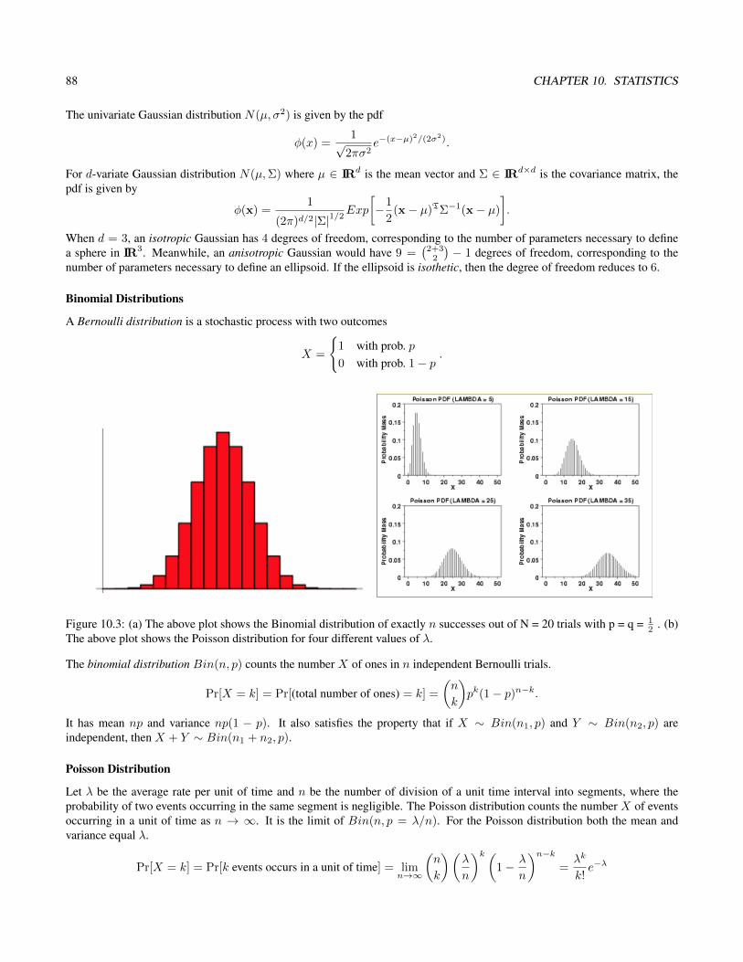
88 CHAPTER 10. STATISTICS
The univariate Gaussian distribution N(µ, σ2) is given by the pdf
φ(x) =1√
2πσ2e−(x−µ)2/(2σ2).
For d-variate Gaussian distribution N(µ,Σ) where µ ∈ IRd is the mean vector and Σ ∈ IRd×d is the covariance matrix, thepdf is given by
φ(x) =1
(2π)d/2|Σ|1/2Exp
[−1
2(x− µ)TΣ−1(x− µ)
].
When d = 3, an isotropic Gaussian has 4 degrees of freedom, corresponding to the number of parameters necessary to definea sphere in IR3. Meanwhile, an anisotropic Gaussian would have 9 =
(2+3
2
)− 1 degrees of freedom, corresponding to the
number of parameters necessary to define an ellipsoid. If the ellipsoid is isothetic, then the degree of freedom reduces to 6.
Binomial Distributions
A Bernoulli distribution is a stochastic process with two outcomes
X =
1 with prob. p0 with prob. 1− p .
Figure 10.3: (a) The above plot shows the Binomial distribution of exactly n successes out of N = 20 trials with p = q = 12 . (b)
The above plot shows the Poisson distribution for four different values of λ.
The binomial distribution Bin(n, p) counts the number X of ones in n independent Bernoulli trials.
Pr[X = k] = Pr[(total number of ones) = k] =
(n
k
)pk(1− p)n−k.
It has mean np and variance np(1 − p). It also satisfies the property that if X ∼ Bin(n1, p) and Y ∼ Bin(n2, p) areindependent, then X + Y ∼ Bin(n1 + n2, p).
Poisson Distribution
Let λ be the average rate per unit of time and n be the number of division of a unit time interval into segments, where theprobability of two events occurring in the same segment is negligible. The Poisson distribution counts the number X of eventsoccurring in a unit of time as n → ∞. It is the limit of Bin(n, p = λ/n). For the Poisson distribution both the mean andvariance equal λ.
Pr[X = k] = Pr[k events occurs in a unit of time] = limn→∞
(n
k
)(λ
n
)k (1− λ
n
)n−k=λk
k!e−λ

10.1. PROBABILITY PRIMER 89
10.1.3 Pairwise independenceA set of events E1, E2, . . . , En are mutually independent if for any subset I ⊆ 1, 2, . . . , n,
Pr
[⋂i∈I
Ei
]=∏i∈I
Pr[Ei].
A set of discrete random variables X1, X2, . . . , Xn are mutually independent if for any subset I ⊆ 1, 2, . . . , n,
Pr
[∧i∈I
Xi = xi
]=∏i∈I
Pr[Xi = xi].
For example, if X = (X1, X2, . . . , Xn) ∼ N(0, I), then Xi ∼ N(0, 1) are mutually independent. If X = (X1, X2, . . . , Xn) isuniformly distributed on the hypercube [0, 1]n, then Xi ∼ U(0, 1) are mutually independent.A set of events E1, E2, . . . , En are k-wise independent if for any subset I ⊆ 1, 2, . . . , n such that |I| ≤ k,
Pr
[⋂i∈I
Ei
]=∏i∈I
Pr[Ei].
A set of discrete random variablesX1, X2, . . . , Xn are k-wise independent if for any subset I ⊆ 1, 2, . . . , n such that |I| ≤ k,
Pr
[∧i∈I
Xi = xi
]=∏i∈I
Pr[Xi = xi].
When k = 2, it is also called pairwise independence. In other words, X1, X2, . . . , Xn are pairwise independent if for all i 6= jand any pair of values (a, b),
Pr[X1 = a ∧X2 = b] = Pr[X1 = a] Pr[X2 = b].
Lemma 10.2 ([85, Lemma 13.1]). We can generate m = 2n − 1 uniform pairwise independent bits from n uniform mutuallyindependent bits. (A random bit is uniform if it assumes values 0 or 1 with equal probability 1/2).
Idea of proof. Generate n uniform random bits X1, X2, . . . , Xn ∈ 0, 1. Enumerate all (2n − 1) non-empty subsets of1, 2, . . . , n. Let Sj be the jth subset of the enumeration. Then, set
Yj =
∑i∈Sj
Xi
mod 2
=⊕i∈Sj
Xi,
where ⊕ denotes XOR.
Lemma 10.3 ([85, Lemma 13.2]). Let X1 and X2 be independent and uniform over GF(p). Generate Yi = (X1 + iX2)mod p for i ∈ 0, 1, 2, p− 1. Then, Y0, Y1, Y2, . . . , Yp−1 are pairwise independent.
Proof. For a given X2, we know that Yi is uniform over GF(p) as X1 is uniform over GF(p).Consider Yi and Yj , where i 6= j. For any a, b ∈ 0, 1, 2, . . . , p− 1,
Yi = X1 + iX2 = a and Yj = X1 + jX2 = b
⇐⇒ X2 =b− aj − i and X1 = a− i(b− a)
j − i .
Hence, Pr[Yi = a ∧ Yj = b] = 1p2 .

90 CHAPTER 10. STATISTICS
Finite Field
Finite fields appear in Rijndael — the AES cryptographic system. The Reed Solomon code uses the Galois field GF(2n), whichis a field of characteristic 2.The field GF(2n) consists over polynomials
P (x) =
n−1∑i=0
cixi (ci ∈ GF(2) = 0, 1)
of degree less than n over the field GF(2) modulo an irreducible polynomial over GF(2). (For example, the polynomialx2 + 2x + 1 = (x + 1)2 is reducible over IR. The polynomial x2 + 1 = (x + i)(x − i) is irreducible over IR, but reducibleover C.)The 2n polynomials can be encoded by 2n strings of bits. For example, x7 + x6 + x4 + 1 can be encoded by the bit string11010001 of length 8.In algebraic geometry, we can study polynomials modulo over the sphere. The famous result of Bézout Theorem says that acurve of degree d and a curve of degree e, with some caveats, intersect at (d · e) points.
10.1.4 Transformation of Random VariablesConsider next a transformation of random variables. We shall revisit the Box-Muller method from lecture 3, and prove that itindeed uniformly samples the Gaussian.Suppose we generate a sample point (X1, X2) according to the joint pdf µ(x1, x2), and then apply an injective function f toobtain (Y1, Y2) = f(X1, X2). It can be shown that the sample (Y1, Y2) follows the joint pdf
ρ(y1, y1) = µ(f−1(y1, y2)) ·∣∣∣∣det
(∂ x
∂ y
)∣∣∣∣,where the Jacobian matrix is defined as
∂ x
∂ y=
(∂ x1
∂ y1∂ x1
∂ y2∂ x2
∂ y1∂ x2
∂ y2
).
Similar techniques also work in IRd.The Box-Muller method transforms a sample point (X1, X2) generated uniformly random from (0, 1)2, and transforms it to
(Y1, Y2) =
(√−2 lnX1 cos(2πX2) ,
√−2 lnX1 sin(2πX2)
).
We now calculate the partial derivatives and verify that the resulting (Y1, Y2) distributes according toN(0, I). First, we expressx1 and x2 in terms of y1 and y2.
x1 = exp(−(y21 + y2
2)/2)
x2 = arctan(y2/y1)/(2π)
Then, we calculate the partial derivatives.
∂ x1
∂ y1= − y1 exp(−(y2
1 + y22)/2)
∂ x1
∂ y2= − y2 exp(−(y2
1 + y22)/2)
∂ x2
∂ y1=
−y2/y21
(2π)(1 + y22/y
21)
∂ x2
∂ y2=
1/y1
(2π)(1 + y22/y
21)
10.1. PROBABILITY PRIMER 91
Hence, the Jacobian determinant is∣∣∣∣∂ x∂ y∣∣∣∣ =
∣∣∣∣∣∂ x1
∂ y1∂ x1
∂ y2∂ x2
∂ y1∂ x2
∂ y2
∣∣∣∣∣=
∣∣∣∣∣−y1 exp(−(y21 + y2
2)/2) −y2 exp(−(y21 + y2
2)/2)−y2/y21
(2π)(1+y22/y21)
1/y1(2π)(1+y22/y
21)
∣∣∣∣∣=
exp(−(y21 + y2
2)/2)
(2π)(1 + y22/y
21)
∣∣∣∣ −y1 −y2
−y2/y21 1/y1
∣∣∣∣=
exp(−(y21 + y2
2)/2)
(2π)(1 + y22/y
21)· (−1− y2
2/y21)
= − exp(−(y21 + y2
2)/2)/(2π)
Therefore, the pdf of (Y1, Y2) is
µ(f−1(y)) ·∣∣∣∣det
(∂ x
∂ y
)∣∣∣∣ = 1 · 1
2πe−(y21+y22)/2 =
1
2πe−(y21+y22)/2,
which shows that (Y1, Y2) ∼ N(0, I).
10.1.5 Annular Concentration of GaussianA one-dimensional Gaussian has its mass close to its mean (Figure 10.1(b)). However, for large d, a d-dimensional GaussianN(0, σ2I) with pdf
p(x) =1
(2π)d/2σde−‖x‖
2/(2σ2)
has very little mass close to the origin, even though its maximum probability density is at the origin. In fact,∫ 1
0
p(r) d r
is vanishing small, where r is the Ell2 distance from the center (Figure 10.4(b)) and p(r) is the marginal probability density(Figure 10.4(c)). For N(0, I), we know that
p(r) ∝ rd−1er2/2.
So, where is the maximum mass? We can set the derivative to zero.
d
d rrd−1er
2/2 = (d− 1)rd−2e−r2/2 − rde−r2/2 = 0
r2 = d− 1
r =√d− 1
So, we need r ≈√d to see significant probability mass. For r
√d, the mass is non-significant. For r
√d, mass also
disappears.
Theorem 10.4 ([18, Theorem 2.9]). Let X = X1 + X2 + . . . + Xn, where Xi are mutually independent with mean 0 andvariance at most σ2. Let 0 ≤ a ≤
√2nσ2. Suppose |E[Xs
i ]| ≤ σ2s! for all 3 ≤ s ≤ (a2/(4nσ2), then
Pr[|X| ≥ a] ≤ 3e−a2/(12nσ2).
We will prove the above theorem in the next lecture, and using Markov inequality. Here we use this theorem to prove themultivariate spherical Gaussian Annulus Theorem. Recall the intimate relationship of the level sets of spherical Gaussian in Rd
and balls in Rd . So similar to the Theorem 2.8 of BHK for unit balls, we discussed in lecture 2, we have

92 CHAPTER 10. STATISTICS
Figure 10.4: (a) A univariate Gaussian concentrated around its mean. (b) Spherical level sets of Ell2 distance. (c) The marginaldistribution p(r) with peak at r =
√d− 1.
Theorem 10.5 (Gaussian Annulus Theorem [18, Theorem 2.8]). For a d-dimensional spherical GaussianN(0, I) and c ≤√d,
all but 3e−c2/96 of the probability mass lies within an annulus of
√d− c ≤ r ≤
√d+ c.
Proof. For a point x = (x1, x2, . . . , xd) ∼ N(0, I), we have
r2 = ‖x‖2 = x21 + x2
2 + . . .+ x2d.
Consider
|r −√d| ≥ c
=⇒ r2 − d = |r −√d| · |r +
√d| ≥ c
√d (since |r +
√d| ≥
√d)
=⇒ |y1 + y2 + . . .+ yd| ≥ c√d (yi = x2
i − 1)
=⇒ |z1 + z2 + . . .+ zd| ≥ c√d/2. (zi = yi/2)
To use the above theorem, we bound the moments of zi using the Gamma integral.
|E[zsi ]| = 2−sE[|yi|s]≤ 2−sE[1 + x2
i ]
= 2−s + 2−s√
2
π
∫ ∞0
x2se−x2/2 dx
= 2−s +1√π
∫ ∞0
us−0.5e−u du (substitue x =√
2u)
≤ s!Hence, we can apply the above theorem with σ2 = E[z2
i ] ≤ 4 and |E[zsi ]| ≤ 4(s!).
Pr[|z1 + z2 + . . .+ zd| ≥ c√d/2] ≤ 3e−c
2/96.
10.1.6 Distribution SamplingHow can we sample points from a given distribution, for example N(0, I)? If x ∈ IR has pdf p(x), then we can define use itscdf
P : IR→ IR
x 7→ P (x) =
∫ x
−∞p(t) d t.

10.1. PROBABILITY PRIMER 93
If u is uniformly sampled from [0, 1], then x = P−1(u) will be distributed according to pdf p(x). So, for d-dimensionalGaussian N(0, I), we can draw u = (u1, u2, . . . , ud) uniformly from [0, 1]d and take inverse of the cdf componentwisex = (x1, x2, . . . , xd) = (P−1(u1), P−1(u2), . . . , P−1(ud)).Another example is the Cauchy distribution with pdf
p(x) =1
π(1 + x2).
Its cdf is given by
P (x) =
∫ x
−∞
1
π(1 + t2)d t =
1
πarctanx+
1
2.
Box-Muller Method
Independent samples X1, X2 ∼ U(0, 1) can be used to generate samples (Y1, Y2) of a bivariate Gaussian distribution N(0, I)using the Box-Muller method as follows.
Y1 =√−2 lnX1 cos(2πX2)
Y2 =√−2 lnX1 sin(2πX2)
Then, we have the following.
X1 = e−(Y 21 +Y 2
2 )/2
X2 = arctan(Y2/Y1)
The Jacobian determinant equals
J =
(1√2πe−y
21/2
)(1√2πe−y
22/2
).
10.1.7 Mixture of Gaussians
x
y
√d
√d
√2d
𝑥
𝑝 𝑞
𝑧
𝑑
2𝑑
𝑦
𝛿
𝛿
𝛿 2 + 2𝑑
Figure 10.5: (a) Nearly orthogonal Gaussian samples x and y. (b) Samples x and y from two Gaussians centered at p and qrespectively.
Given a mixture of two Gaussian densitiesp(x) = w1p1(x) + w2p2(x),
where w1 + w2 = 1 is a convex combination. It can be shown that if the means of the d-dimension spherical unit-varianceGaussians are separated by Ω(d1/4), then they are separable. The idea is that with high probability, points in the same clusterbelong to the same Gaussian because most of the points are concentrated. More formally, with high probability ‖x − y‖2 =

94 CHAPTER 10. STATISTICS
2d ± O(√d) if they come from the same Gaussian, and ‖x − y‖2 = δ2 + 2d ± O(
√d) if they come from different Gaussian
separated by δ.Suppose x,y ∼ N(µ, I) come from the same Gaussian (Figure 10.5(a)). Observe that most probability mass lies in an annulusof width O(1) and radius
√d− 1. Rotate the coordinate system so that x is at the North pole. With high probability, y is in the
slab (y1, y2, . . . , yd) : −c ≤ y1 ≤ c for some c ∈ O(1). So, y is nearly orthogonal to x and hence ‖x−y‖ ≈√‖x‖2 + ‖y‖2.
More precisely, we can further rotate the coordinate system so that
x = (√d±O(1), 0, 0, . . . , 0) and y = (±O(1),
√d±O(1), 0, . . . , 0).
Hence, ‖x− y‖2 = (d±O(√d)) + (d±O(
√d)) = 2d±O(
√d). See also (Figure 10.5(b))
Suppose x ∼ N(p, I) and y ∼ N(q, I) come from different Gaussians . With high probability, x and y lies in an annulusof of width O(1) and radius
√d− 1 centered at p and q respectively. Also, (x − p), (p − q), (q − y) are nearly mutually
perpendicular. Hence, ‖x− y‖2 ≈ ‖x− p‖2 + δ2 + ‖q− y‖2 = δ2 + 2d±O(√d).
Thus, if δ = Ω(d1/4), we can separable constant number of points with constant failure probability.In general, we can ask the question of separating many Gaussians. It can be solved if they are well-separated. One applicationof separating a mixture of Gaussians is in locating the position of atoms by sampling, which is possible if the separation ofatoms in the lattice is large enough.
10.1.8 Concentration Theorems
The following probability inequalities by Markov and Chebyshev are used to prove the Law of Large Numbers.
Theorem 10.6 (Markov Inequality [18, Theorem 2.1] [85, Theorem 3.1]). Let X ≥ 0 be a random variable and a > 0.
Pr[X ≥ a] ≤ E[X]/a.
Proof. For a continuous non-negative random variable x with probability density p(x)
E[X] =
∫ ∞0
xp(x) dx
=
∫ a
0
xp(x) dx+
∫ ∞a
xp(x) dx
≥∫ ∞a
xp(x) dx
≥∫ ∞a
ap(x) dx
= a
∫ ∞a
p(x) dx
= aPr[X ≥ a]
Note the proof works for discrete probability distributions. Replace summations for all the integrals.
Corollary 10.7. Let X be a non-negative random variable and c > 0. Then, Pr[X ≥ cE[X]] ≤ 1/c.
The above says that the value of X is not far from the mean E(X). The Chebyshev’s inequality (below) can be proved byapplying Markov’s inequality on the variance.
Theorem 10.8 (Chebyshev Inequality [18, Theorem 2.3] [85, Corollary 3.7]). Let X be a random variable with mean m andvariance σ2. Then, for all a > 0,
Pr[ |X −m| ≥ aσ ] ≤ 1/a2.
Using the Chebyshev inequality, we can now prove the Law of Large Numbers.

10.1. PROBABILITY PRIMER 95
Theorem 10.9 (Law of Large Numbers). Let S be the sample mean of n independent random variables X1, X2, . . . , Xn withmeans E[Xi] = m and variances Var[Xi] = σ2. Then, for all ε > 0,
Pr[|S −m| ≥ ε] ≤ σ2
nε2.
Proof. Applying Chebyshev Inequality on S with a = ε/σ(S), we get
Pr [|S −m| ≥ ε] ≤ σ2(S)/ε2
=1
ε2σ2
(X1 +X2 + . . .+Xn
n
)=
1
n2ε2σ2(X1 +X2 + . . .+Xn)
=σ2
nε2.
10.1.9 Application of Markov and Chebyshev Inequalities
Theorem 10.10 ([18, Theorem 2.9]). Let X = X1 + X2 + . . . + Xn, where Xi are mutually independent with mean 0 andvariance at most σ2. Let 0 ≤ a ≤
√2nσ2. Suppose |E[Xs
i ]| ≤ σ2s! for all 3 ≤ s ≤ (a2/(4nσ2), then
Pr[|X| ≥ a] ≤ 3e−a2/(12nσ2).
Proof. We will bound |E[Xr]| and use Markov inequality.Consider the expansion
(X1 +X2 + . . .+Xn)r =∑
∑ri=r
(r
r1 r2 . . . rn
)Xr1
1 Xr22 . . . Xrn
n ,
where(
rr1 r2 ... rn
)= r!
r1!·r2!·...·rn! .Since Xi are independent,
E
[(X1 +X2 + . . .+Xn)r
]=
∑∑ri=r
(r
r1 r2 . . . rn
)E[Xr1
1 ] E[Xr22 ] . . .E[Xrn
n ].
Note that E[Xi] = 0. So, all terms with ri = 1 are zero. So, all non-zero terms have ri ≥ 2 or ri = 0. Since∑i ri = r, this
implies that in a non-zero term, there are at most r/2 non-zero indices ri.The number of non-zero terms with exactly t indices ri ≥ 2 equals(
n
t
)(r − t− 1
t− 1
),
because there are(nt
)ways to choose a subset of 1, 2, . . . , n of cardinality t corresponding to the t indices with weight at least
2, and there are(
(r−2t)+(t−1)t−1
)=(r−t−1t−1
)ways to allocate the remaining (n− 2t) weights. (This is analogous to the fact that
the number of monic monomials in a polynomial of degree at most e = r − 2t in n = t− 1 variables equals(e+nn
)=(e+ne
).)
Also using |E[Xi]ri | ≤ σ2ri!, we get
E[Xr] ≤ r!r/2∑t=1
(n
t
)(r − t− 1
t− 1
)σ2t
≤ r!r/2∑t=1
(nσ2)t
t!2r−t−1.

96 CHAPTER 10. STATISTICS
Let h(t) = (nσ2)t
t! 2r−t−1. Since a ≤√
2nσ2 and s ≤ a2/(4nσ2), we have r ≤ s ≤ nσ2/2. For t ≤ r/2, increasing t by 1increases h(t) by nσ2/(2t) ≥ 2. Thus,
E[Xr] ≤ r!r/2∑t=1
h(t)
≤ r! · h(r
2
)(1 +
1
2+
1
4+ . . .
)≤ r! · (nσ2)r/2
(r/2)!2r/2.
Applying the Markov Inequality, we get
Pr[|X| ≥ a] = Pr[Xr ≥ ar] ≤ r! · (nσ2)r/2 · 2r/2(r/2)! · ar ≤
(2nrσ2
a2
)r/2.
Setting r to be the largest even integer less than a2/(6nσ2) completes the proof.
Lemma 10.11. For any integer s > 0, the sth moment of X ∼ N(0, 1) is at most (s!).
Proof. It follows from the following integral.
E[Xs] =
∫ +∞
−∞
xs√2πe−x
2/2 dx =
0 if s is odd(s− 1)!! if s is even
10.1.10 Chernoff BoundsRecall the binomial distribution Bin(n, p) counts the number X of ones in n independent Bernoulli trials.
Pr[X = k] = Pr[(total number of ones) = k] =
(n
k
)pk(1− p)n−k.
It can be written as a sum X =∑Xi of Bernoulli random variables Xi with parameter p, in other words,
Xi =
0 with prob. (1− p)1 with prob. p the ith trial is a success
.
It has expectation E[X] = np and variance Var[X] = np(1− p). What we desire is a bound on the probability that the sumrandom variable X , does not deviate too far from this expected value.What we next present is a general technique to compute such probability bounds.The Chernoff bounds [18, Theorem 12.3 & Theorem 12.4] [85, Theorem 4.4 & Theorem 4.5] say that for all δ > 0,
Pr[X > (1 + δ)m] ≤[
eδ
(1 + δ)1+δ
]m,
and for all 0 ≤ γ ≤ 1,Pr[X < (1− γ)m] ≤ e−γ2m/2,
where X =∑iXi and m = E[X].
For several NP-hard problems, we can use input or data sampling to obtain a probabilistic approximation algorithm. We can thenapply Markov, Chebyshev and Chernoff tail bounds. Sometimes, we can also weaken the assumption of mutually independentsample to k-wise independence (e.g. k = 2). More on this in the next lecture.In Monte Carlo methods, we use random sampling. In Quasi Monte Carlo, we use deterministic methods and measure thedistortion from uniformity by discrepancy (for example, by considering the family of isothetic rectangles). See for e.g. [?]There are also methods known as Markov Chain Monte Carlo (MCMC) or Markov Chain Quasi Monte Carlo (MCQMC).

10.2. BAYESIAN 97
Estimating π
We can use the Monte Carlo method to estimate π. Sample z1, z2, . . . , zm independently and uniformly from [0, 1]2. Defineindicator random variables
Zi =
1 if ‖zi‖2 ≤ 1
0 otherwise.
Then,
Pr[Zi = 1] =(area of the unit circle inside [0, 1]2)
(area of the unit square)=π
4.
Let W =∑mi=1 Zi. Then,
E[W ] =
m∑i=1
E[Zi] =mπ
4.
Let W ′ = 4mW . Then, E[W ′] = π. Hence, W ′ gives an estimate for π.
In fact, it improves as m gets larger. By the Chernoff inequality bounds, we get
Pr[|W − E[W ]| ≥ εE[W ]] ≤ 2e−mπε2/12.
For ε < 1, we can choose m ≥ 12πε2 ln 2
δ . Then, the above algorithm is an (ε, δ)-approximation.
Probabilistic Approximation Algorithm
A randomized algorithm gives an (ε, δ)-approximation for a value v if the output X of the algorithm satisfies
Pr[|X − v| ≤ εv] ≥ 1− δ.
Theorem 10.12 ([85, Theorem 10.1]). Let X1, X2, . . . , Xm be i.i.d. indicator random variables with µ = E[Xi]. If m ≥3ε2µ ln 2
δ , then Pr[∣∣( 1
m
∑mi=1Xi
)− µ
∣∣ ≥ εµ] ≤ δ. That is, an m-sampling provides an (ε, δ)-approximation.
Proof. This can be proved using the above stated Chernoff bound.
10.2 Bayesian
10.2.1 Bayes RuleWe will learn to use probability theory to use sampling for parameter estimation. Consider the Bayes rule.
Pr[A|B] =Pr[B|A] Pr[A]
Pr[B]
This follows from Pr[A|B] Pr[B] = Pr[B|A] Pr[A]. We can regard B as the measurement samples that we have. Using thisdata, we try to estimateA. In the numerator, Pr[B|A] is the likelihood ofA and Pr[A] is the prior probability. The normalizationappears in the denominator Pr[B]. The left hand side is the posterior probability Pr[A|B].For example, suppose that a product is defective 0.1% of the time, and a test fails 1% of the time to detect a defective product.Also, assuming that a product is not defective, a test says a product is defective 2% of the time.Let A be the event that a product is defective. Let B be the event that a test says a product is defective. Then, we have thefollowings.
Pr[B|A] = 0.99
Pr[A] = 0.001
Pr[B|A] = 0.02
Pr[B] = Pr[B|A] Pr[A] + Pr[B|A] Pr[A] = 0.99× 0.001 + 0.02× 0.999 = 0.02097
98 CHAPTER 10. STATISTICS
So, using the Bayes rule, we can estimate
Pr[A|B] =Pr[B|A] Pr[A]
Pr[B]=
0.99× 0.001
0.0297≈ 0.047,
which is surprising.The Bayes rule can be applied to molecule reconstruction from projection images. In such applications, the molecule imagingis used to reconstruct the structure of the molecule. This is analogous to using measurements to make estimations according tothe Bayes rule.
10.2.2 Maximum Likelihood EstimatorSuppose a probability distribution of a random variable X depends on parameter r. So, Pr[X|r] denotes the probability ofobserving X if parameter value is r. If r is also random, after observing the value of X , one can find the best r maximizing theposterior probability
Pr[r|X] =Pr[X|r] Pr[r]
Pr[X].
Assume Pr[r] is the same for all r. Since the unconditional probability of X in the denominator is independent of r, it reducesto finding the maximum likelihood estimator (MLE)
arg maxr
L(r|X) = arg maxr
Pr[X|r].
ExampleConsider the example of flipping a biased coin in n trials with unknown probability r of getting head. The probability of gettingk heads follows the binomial disbtribution Bin(n, r) such that
Pr[k|r] =
(n
k
)rk(1− r)n−k.
If we get 62 heads and 38 tails in 100 trails, the maximum likelihood estimator gives r = 0.62 when Pr[62|r] is maximized.One can see this by setting the derivative (with respect to r) to 0.We can study a single particle using cryo-electron microscopy. To do so, we build a specimen grid of millions of in-vitromolecules and take a snapshot by shooting X-ray and measuring its projection. We can reconstruct the locations of the moleculesby solving a least square optimization with regularizer, but it is unstable. How many samples would we need? We want to showthat the solution converges as the sample size increase. We can recast the problem by regarding the data as a random variablewith certain mean and variance. We can then solve for the maximum a-posterior estimator. We would also like to output aconfidence level of our estimation.
10.2.3 Unbiased EstimatorLet X = (X1, X2, . . . , Xn) be samples or observations from a distribution having parameter θ. (For example, the Gaussiandistribution N(µ, σ2) has parameters mean µ and variance σ2, while the binomial distribution Bin(n, p) has parameters n andsuccess probability p.)Let D(X) be an estimator of some function h(θ). The bias is defined as
E[D(X)− h(θ)].
It is called an unbiased estimator when the bias equals zero.The quality of the estimator can be measured by the mean squared error (MSE)
E[(D(X)− h(θ))2] = Var(D(X)) + Bias2.
Theorem 10.13. Let X1, X2, . . . , Xn be independent samples, each with mean µ and variance σ2.
B1. [?, Example 14.3] D(X) = 1n
∑ni=1Xi is an unbiased estimator of µ.

10.3. BIOLOGICAL APPLICATIONS 99
B2. If µ is known, then D(X) = 1n
∑ni=1(Xi − µ)2 is an unbiased estimator of σ2.
B3. [?, Example 14.5] If µ is not known, then D(X) = 1n−1
∑ni=1(Xi −m)2 is an unbiased estimator of σ2, where m =
1n
∑ni=1Xi.
Proof of 3. Let S2 = 1n
∑ni=1(Xi −m)2. Observe that
n∑i=1
(Xi − µ)2 =
n∑i=1
[(Xi −m) + (m− µ)
]2
=
n∑i=1
(Xi −m)2 + n(m− µ)2
Hence,
S2 =1
n
n∑i=1
(Xi −m)2
=1
n
n∑i=1
(Xi − µ)2 − (m− µ)2
E[S2] =1
n
n∑i=1
Var(Xi)−Var(m)
=n− 1
nσ2
Thus,(
nn−1S
2)
is an unbiased estimator of σ2.
10.3 Biological Applications
Summary
References and Further ReadingExerSection

100 CHAPTER 10. STATISTICS

Biology Appendix
101

102 CHAPTER 10. STATISTICS

Conclusions
Something to conclude
103

104 CHAPTER 10. STATISTICS

Bibliography
[1] S. S. Abhyankar and C. L. Bajaj. Automatic parameterization of rational curves and surfaces III: algebraic plane curves.Comput. Aided Geom. Des., 5(4):309–321, 1988.
[2] R. Abraham, J. E. Marsden, and T. Ratiu. Manifolds, tensor analysis, and applications, volume 75 of Applied Mathe-matical Sciences. Springer-Verlag, New York, second edition, 1988.
[3] N. Akkiraju and H. Edelsbrunner. Triangulating the surface of a molecule. Discrete Applied Mathematics, 71(1-3):5–22,1996.
[4] G. Albers and T. Roos. Voronoi diagrams of moving points in higher dimensional spaces. In Proc. 3rd Scand. WorkshopAlgorithm Theory, volume 621 of Lecture Notes in Computer Science, pages 399–409. Springer-Verlag, 1992.
[5] M. A. Armstrong. Basic Topolgy. Springer, New York, 1983.
[6] D. Arnold, R. Falk, and R. Winther. Finite element exterior calculus: from Hodge theory to numerical stability. Bulletinof the American Mathematical Society, 47(2):281–354, 2010.
[7] F. Aurenhammer. Voronoi diagrams: A survey of a fundamental geometric data structure. ACM Computing Surveys,23:345–405, 1991.
[8] C. Bajaj, F. Bernardini, and G. Xu. Automatic reconstruction of surfaces and scalar fields from 3D scans. In ACMSIGGRAPH, pages 109–118, 1995.
[9] C. Bajaj and W. J. Bouma. Dynamic Voronoi diagrams and Delaunay triangulations. In Proceedings of the 2nd CanadianConference on Computational Geometry, pages 273–277, 1990.
[10] C. Bajaj and S. Goswami. Automatic fold and structural motif elucidation from 3d em maps of macromolecules. InICVGIP 2006, pages 264–275, 2006.
[11] C. Bajaj, H. Y. Lee, R. Merkert, and V. Pascucci. NURBS based B-rep models for macromolecules and their properties.In Proceedings of the 4th ACM Symposium on Solid Modeling and Applications, pages 217–228, New York, NY, USA,1997. ACM.
[12] C. Bajaj, V. Pascucci, A. Shamir, R. Holt, and A. Netravali. Multiresolution molecular shapes. Technical report, TICAM,Univ. of Texas at Austin, Dec. 1999.
[13] C. Bajaj, V. Pascucci, A. Shamir, R. Holt, and A. Netravali. Dynamic maintenance and visualization of molecularsurfaces. Discrete Applied Mathematics, 127(1):23–51, 2003.
[14] C. Bajaj, G. Xu, and Q. Zhang. A fast variational method for the construction of resolution adaptive c2-smooth molecularsurfaces. Computer Methods in Applied Mechanics and Engineering, 198(21-26):1684–1690, 2009.
[15] N. Basdevant, D. Borgis, and T. Ha-Duong. A coarse-grained protein-protein potential derived from an all-atom forcefield. Journal of Physical Chemistry B, 111(31):9390–9399, 2007.
[16] M. Behzad and G. Chartrand. Introduction to the theory of graphs. Allyn and Bacon Inc., Boston, Mass., 1971.
[17] J. F. Blinn. A generalization of algebraic surface drawing. ACM Transactions on Graphics, 1(3):235–256, July 1982.
105
106 BIBLIOGRAPHY
[18] A. Blum, J. Hopcroft, and R. Kannan. Foundations of data science. Vorabversion eines Lehrbuchs, 2016.
[19] A. I. Bobenko. Delaunay triangulations of polyhedral surfaces, a discrete laplace-beltrami operator and applications. InSCG ’08: Proceedings of the twenty-fourth annual symposium on Computational geometry, pages 38–38, New York,NY, USA, 2008.
[20] A. Bossavit. Whitney forms: a class of finite elements for three-dimensional computations in electromagnetism. Proc.of the IEEE, 135(8):493–500, 1988.
[21] Y. Bourne, J. Grassi, P. E. Bougis, and P. Marchot. Conformational flexibility of the acetylcholinesterase tetramersuggested by x-ray crystallography. Journal of Biological Chemistry, 274(43):30370–30376, 1999.
[22] Y. Bourne, P. Taylor, and P. Marchot. Acetylcholinesterase inhibition by fasciculin: crystal structure of the complex.Cell, 83:503, 1995.
[23] J. Canny. Generalised characteristic polynomials. Journal of Symbolic Computation, 9(3):241–250, 1990.
[24] F. Cazals, F. Chazal, and T. Lewiner. Molecular shape analysis based upon the morse-smale complex and the connollyfunction. In 19th Ann. ACM Sympos. Comp. Geom., pages 351–360, 2003.
[25] R. Chaine. A geometric convection approach of 3D reconstruction. In Proc. Eurographics Sympos. on Geometry Pro-cessing, pages 218–229, 2003.
[26] G. Chartrand and L. Lesniak. Graphs & digraphs. Chapman & Hall/CRC, Boca Raton, FL, fourth edition, 2005.
[27] F. Chazal and A. Lieutier. Stability and homotopy of a subset of the medial axis. In Proc. 9th ACM Sympos. SolidModeling and Applications, pages 243–248, 2004.
[28] L. P. Chew. Constrained Delaunay triangulations. In Proc. 3rd Annual ACM Symposium Computational Geometry, pages215–222, 1987.
[29] P. Chew. Near-quadratic bounds for the L1 Voronoi diagram of moving points. Computational Geometry Theory andApplications, 7, 1997.
[30] Cocone. Tight Cocone Software for surface reconstruction and medial axis approximation. http://www.cse.ohio-state.edu/∼tamaldey/cocone.html, 2001.
[31] M. Connolly. Solvent-accessible surfaces of proteins and nucleic acids. Science, 221(4612):709–713, 19 August 1983.
[32] M. L. Connolly. Analytical molecular surface calculation. Journal of Applied Crystallography, 16:548–558, 1983.
[33] CVC, UT Austin. Volrover. http://cvcweb.ices.utexas.edu/software/guides.php, 2011.
[34] M. de Berg and K. T. G. Dobrindt. On levels of detail in terrains. Graphical Models and Image Processing, 60:1–12,1998.
[35] M. Desbrun and M. Gascuel. Animating soft substances with implicit surfaces. In R. Cook, editor, SIGGRAPH 95Conference Proceedings, Annual Conference Series, pages 287–290, Los Angeles, August 1995. Addison Wesley.
[36] T. K. Dey, J. Giesen, and S. Goswami. Shape segmentation and matching with flow discretization. In F. Dehne, J.-R.Sack, and M. Smid, editors, Proc. Workshop Algorithms Data Strucutres (WADS 03), LNCS 2748, pages 25–36, Berlin,Germany, 2003.
[37] M. Eck, T. DeRose, T. Duchamp, T. Hoppe, H. Lounsbery, and W. Stuetzle. Multiresolution analysis of arbitrary meshes.In ACM Computer Graphics Proceedings, SIGGRAPH’95, pages 173–180, 1995.
[38] H. Edelsbrunner. Weighted alpha shapes. Technical Report 1760, University of Illinois at Urbana-Champaign, 1992.
[39] H. Edelsbrunner. Surface reconstruction by wrapping finite point sets in space. In B. Aronov, S. Basu, J. Pach, andM. Sharir, editors, Ricky Pollack and Eli Goodman Festschrift, pages 379–404. Springer-Verlag, 2002.

BIBLIOGRAPHY 107
[40] H. Edelsbrunner, M. Facello, and J. Liang. On the definition and the construction of pockets in macromolecules. TechReport UIUCDCS-R-95-1935, University of Illinois Urbana-Champaign, 1995.
[41] H. Edelsbrunner, J. Harer, V. Natarajan, and A. Zomorodian. Morse-smale complexes for piecewise linear 3-manifolds.In 19th Ann. Sympos. Comp. Geom., pages 361–370, 2003.
[42] H. Edelsbrunner, J. Harer, and A. Zomorodian. Hierarchical morse-smale complexes for piecewise linear 2-manifolds.Discrete Computational Geometry, 30:87–107, 2003.
[43] H. Edelsbrunner and E. P. Mücke. Three-dimensional alpha shapes. ACM Transactions on Graphics, 13(1):43–72, 1994.
[44] H. Edelsbrunner and N. R. Shah. Incremental topological flipping works for regular triangulations. Algorithmica,15:223–241, 1996.
[45] E. Eyal and D. Halperin. Dynamic maintenance of molecular surfaces under conformational changes. In SCG ’05:Proceedings of the 21st Annual Symposium on Computational Geometry, pages 45–54, 2005.
[46] E. Eyal and D. Halperin. Improved maintenance of molecular surfaces using dynamic graph connectivity. Algorithms inBioinformatics, pages 401–413, 2005.
[47] M. A. Facello. Geometric Techniques for Molecular Shape Analysis. PhD thesis, University of Illinois, 1996. Departmentof Computer Science Technical Report # 1967.
[48] J. J. Fu and R. C. T. Lee. Voronoi diagrams of moving points in the plane. International Journal of ComputationalGeometry Applications, 1(1):23–32, 1991.
[49] T. Fujita, K. Hirota, and K. Murakami. Representation of splashing water using metaball model. Fujitsu, 41(2):159–165,1990. in Japanese.
[50] M. Garland. QSlim. http://graphics.cs.uiuc.edu/ garland/software/qslim.html, 2004.
[51] M. Garland and P. Heckbert. Simplifying surfaces with color and texture using quadric error metrics. In IEEE Visualiza-tion, pages 263–270, 1998.
[52] P. Giblin. Graphs, surfaces and homology. Cambridge University Press, Cambridge, third edition, 2010.
[53] T. S. Gieng, B. Hamann, K. I. Joy, G. L. Schussman, and I. J. Trotts. Constructing hierarchies for triangle meshes. IEEETransactions on Visualization and Computer Graphics, 4(2):145–161, 1998.
[54] J. Giesen and M. John. The flow complex: a data structure for geometric modeling. In Proc. 14th ACM-SIAM Sympos.Discrete Algorithms, pages 285–294, 2003.
[55] S. Goswami, T. K. Dey, and C. L. Bajaj. Identifying flat and tubular regions of a shape by unstable manifolds. In Proc.11th ACM Sympos. Solid and Phys. Modeling, pages 27–37, 2006.
[56] V. Gradinaru. Whitney elements on sparse grids. PhD thesis, Universität Tübingen, 2002.
[57] V. Gradinaru and R. Hiptmair. Whitney elements on pyramids. Electronic Transactions on Numerical Analysis, 8:154–168, 1999.
[58] R. L. Graham and P. Hell. On the history of the minimum spanning tree problem. Ann. Hist. Comput., 7(1):43–57, 1985.
[59] J. Grant and B. Pickup. A gaussian description of molecular shape. Journal of Physical Chemistry, 99:3503–3510, 1995.
[60] G. Graves. The magic of metaballs. Computer Graphics World, 16(5):27–32, 1993.
[61] X. Gu and S.-T. Yau. Global conformal surface parameterization. In SGP ’03: Proceedings of the 2003 Eurograph-ics/ACM SIGGRAPH symposium on Geometry processing, pages 127–137, Aire-la-Ville, Switzerland, Switzerland,2003. Eurographics Association.

108 BIBLIOGRAPHY
[62] L. Guibas, J. S. B. Mitchell, and T. Roos. Voronoi diagrams of moving points in the plane. In Proceedings of the17th Internatational Workshop on Graph-Theoretical Concepts in Computer Science, volume 570 of Lecture Notes inComputer Science, pages 113–125. Springer-Verlag, 1991.
[63] V. Guillemin and A. Pollack. Differential Topology. Prentice-Hall, Inc., Englewood Cliffs, New Jersey, 1974.
[64] R. Hiptmair. Finite elements in computational electromagnetism. Acta Numerica, pages 237–339, 2002.
[65] A. N. Hirani. Discrete Exterior Calculus. PhD thesis, California Institute of Technology, 2003.
[66] C. Ho and C. Yap. Polynomial Remainder Sequences and Theory of Subresultants. Technical report, Technical Report,1987.
[67] M. Holst, N. Baker, and F. Wang. Adaptive multilevel finite element solution of the poisson-boltzmann equation i:Algorithms and examples. Journal of Compututational Chemistry, 21:1319–1342, 2000.
[68] H. Hoppe. Progressive meshes. In ACM Computer Graphics Proceedings, SIGGRAPH’96, pages 99–108, 1996.
[69] P. H. Hubbard. Collision Detection for Interactive Graphics Applications. PhD thesis, Department of Computer Science,Brown University, Providence, Rhode Island, April 1995.
[70] P. M. Hubbard. Approximating polyhedra with spheres for time-critical collision detection. ACM Transactions onGraphics, 15(3), 1996.
[71] H. Imai, M. Iri, and K. Murota. Voronoi diagram in the laguerre geometry and its applications. SIAM J. Comput.,14:93–10, 1985.
[72] P. Jain, P. Kar, et al. Non-convex optimization for machine learning. Foundations and Trends R© in Machine Learning,10(3-4):142–336, 2017.
[73] T. Ju, F. Losasso, S. Schaefer, and J. Warren. Dual contouring of hermite data. In SIGGRAPH, pages 339–346, 2002.
[74] A. Khodakovsky, N. Litke, and P. Schroder. Globally smooth parameterizations with low distortion. ACM Transactionson Graphics, 22(3):350–357, 2003.
[75] R. Klein and J. Kramer. Multiresolution representations for surface meshes. In Proceedings of the SCCG, 1997.
[76] J. B. Kruskal, Jr. On the shortest spanning subtree of a graph and the traveling salesman problem. Proc. Amer. Math.Soc., 7:48–50, 1956.
[77] S. Kumar, D. Manocha, and A. Lastra. Interactive display of large-scale NURBS models. IEEE Transactions on Visual-ization and Computer Graphics, 2(4):323–336, 1996.
[78] M. Lee, M. Feig, F. Salsbury, and C. Brooks. New analytic approximation to standard molecular volume definition andits application to generalized born calculation. Journal of Computational Chemistry, 24:1348–1356, 2003.
[79] M. Levitt, C. Sander, and P. S. Stern. Protein normal-mode dynamics: Trypsin inhibitor, crambin, ribonuclease andlysozyme. Journal of Molecular Biology, 181:423 – 447, 1985.
[80] R. Loos. Generalized Polynomial Remainder Sequences, 1983.
[81] F. Macaulay. Some formulae in elimination. Proceedings of the London Mathematical Society, 1(1):3, 1902.
[82] A. Maheshwari, P. Morin, and J. R. Sack. Progressive tins: Algorithms and applications. In Proceedings 5th ACMWorkshop on Advances in Geographic Information Systems, Las Vegas, 1997.
[83] N. L. Max. Computer representation of molecular surfaces. IEEE Computer Graphics and Applications, 3(5):21–29,August 1983.
[84] J. Milnor. Morse Theory. Princeton University Press, New Jersey, 1963.

BIBLIOGRAPHY 109
[85] M. Mitzenmacher and E. Upfal. Probability and computing: Randomized algorithms and probabilistic analysis. Cam-bridge university press, 2005.
[86] J. R. Munkres. Elements of algebraic topology. Addison-Wesley Publishing Company, Menlo Park, CA, 1984.
[87] J.-C. Nédélec. Mixed finite elements in R3. Numer. Math., 35(3):315–341, 1980.
[88] J.-C. Nédélec. A new family of mixed finite elements in R3. Numer. Math., 50(1):57–81, 1986.
[89] H. Nishimura, M. Hirai, T. Kawai, T. Kawata, I. Shirakawa, and K. Omura. Object modeling by distribution functionand a method of image generation. Transactions IECE Japan, Part D, J68-D(4):718–725, 1985.
[90] T. Nishita and E. Nakamae. A method for displaying metaballs by using Bézier clipping. In Computer Graphics Forum,volume 13, pages 271–280. Eurographics, Basil Blackwell Ltd, 1994. Eurographics ’94 Conference issue.
[91] P.-A. Raviart and J. M. Thomas. A mixed finite element method for 2nd order elliptic problems. In Mathematical aspectsof finite element methods (Proc. Conf., Consiglio Naz. delle Ricerche (C.N.R.), Rome, 1975), pages 292–315. LectureNotes in Math., Vol. 606. Springer, Berlin, 1977.
[92] J. Renegar. On the computational complexity and geometry of the first-order theory of the reals. Part I: Introduction.Preliminaries. The geometry of semi-algebraic sets. The decision problem for the existential theory of the reals. Journalof symbolic computation, 13(3):255–299, 1992.
[93] T. Roos. Voronoı diagrams over dynamic scenes. Discrete Applied Mathematics. Combinatorial Algorithms, Optimiza-tion and Computer Science, 43(3):243–259, 1993.
[94] T. Roos. New upper bounds on Voronoi diagrams of moving points. Nordic Journal of Computing, 4(2):167–171, 1997.
[95] K. Rosen. Discrete mathematics and its applications. McGraw-Hill, 2003.
[96] J. Rossignac and P. Borrel. Multi-resolution 3d approximation for rendering complex scenes. In B. Falcidieno andT. Kunii, editors, Geometric Modeling in Computer Graphics, pages 455–465. Springer-Verlag, 1993.
[97] G. Salmon. Lessons introductory to the modern higher algebra. Hodges, Figgis, and co., 1885.
[98] M. Sanner, A. Olson, and J. Spehner. Fast and robust computation of molecular surfaces. In Proceedings of the eleventhannual symposium on Computational geometry, pages 406–407. ACM Press, 1995.
[99] M. Sanner, A. Olson, and J. Spehner. Reduced surface: an efficient way to compute molecular surfaces. Biopolymers,38(3):305–320, March 1996.
[100] M. F. Sanner and A. J. Olson. Real time surface reconstruction for moving molecular fragments. In Proceedings of thePacific Symposium on Biocomputing ’97, Maui, Hawaii, January 1997.
[101] J. Schreiner, A. Asirvatham, E. Praun, and H. Hoppe. Inter-surface mapping. In ACM Transactions on Graphics (TOG),volume 23, pages 870–877. ACM, 2004.
[102] W. J. Schroeder. A topology modifying progressive decimation algorithm. In R. Yagel and H. Hagen, editors, IEEEVisualization ’97, pages 205–212. IEEE, nov 1997.
[103] A. Sheffer, E. Praun, and K. Rose. Mesh parameterization methods and their applications. Foundations and Trends R© inComputer Graphics and Vision, 2(2):105–171, 2006.
[104] D. Siersma. Voronoi diagrams and morse theory of the distance function. In O. E. Barndorff and E. B. V. Jensen, editors,Geometry in Present Day Science, pages 187–208. World Scientific, 1999.
[105] I. Sloan. Integration and approximation in high dimensions–a tutorial. Uncertainty Quantification, Edinburgh, 2010.
[106] Y. Song, Y. Zhang, C. Bajaj, and N. Baker. Continuum diffusion reaction rate calculations of wild type and mutant mouseacetylcholinesterase: Adaptive finite element analysis. Biophysical Journal, 87(3):1558–1566, 2004.

110 BIBLIOGRAPHY
[107] Y. Song, Y. Zhang, T. Shen, C. Bajaj, J. McCammon, and N. Baker. Finite element solution of the steady-state smolu-chowski equation for rate constant calculations. Biophysical Journal, 86(4):2017–2029, 2004.
[108] O. G. Staadt and M. H. Gross. Progressive tetrahedralizations. In Proceddings of the IEEE Visualization Conference,pages 397–402, 1998.
[109] F. Tama. Normal mode analysis with simplified models to investigate the global dynamics of biological systems. Proteinand Peptide Letters, 10(2):119 – 132, 2003.
[110] A. Varshney and F. Brooks. Fast analytical computation of richards’s smooth molecular surface. In VIS ’93: Proceedingsof the 4th conference on Visualization ’93, pages 300–307, 1993.
[111] R. Voorintholt, M. T. Kosters, G. Vegter, G. Vriend, and W. G. Hol. A very fast program for visualizing protein surfaces,channels and cavities. Journal of Molecular Graphics, 7(4):243–245, December 1989.
[112] R. Walker. Algebraic Curves. Springer Verlag, New York, 1978.
[113] H. Whitney. Geometric Integration Theory. Princeton University Press, 1957.
[114] J. B. with C. Bajaj, J. Blinn, M.-P. Cani-Gascuel, A. Rockwood, B. Wyvill, and G. Wyvill, editors. Introduction toImplicit Surfaces. Morgan Kaufmann Publishers, San Francisco, 1997.
[115] B. Wyvill, C. McPheeters, and G. Wyvill. Animating soft objects. The Visual Computer, 2(4):235–242, 1986.
[116] B. Wyvill, C. McPheeters, and G. Wyvill. Data structure for soft objects. The Visual Computer, 2(4):227–234, 1986.
[117] S. Yoshimoto. Ballerinas generated by a personal computer. Journal of Visualization and Computer Animation, 3(2):55–90, 1992.
[118] T. You and D. Bashford. An analytical algorithm for the rapid determination of the solvent accessibility of points in athree-dimensional lattice around a solute molecule. Journal of Computational Chemistry, 16(6):743–757, 1995.
[119] Z. Yu and C. Bajaj. A segmentation-free approach for skeletonization of gray-scale images via anisotropic vector dif-fusion. Computer Vision and Pattern Recognition, 2004. CVPR 2004. Proceedings of the 2004 IEEE Computer SocietyConference on, 1:I–415–I–420 Vol.1, 2004.
[120] D. Zhang, J. Suen, Y. Zhang, Y. Song, Z. Radic, P. Taylor, M. Holst, C. Bajaj, N. Baker, and J. McCammon. Tetramericmouse acetylcholinesterase: Continuum diffusion rate calculations by solving the steady-state smoluchowski equationusing finite element methods. Biophysical Journal, 88(3):1659–1665, 2004.
[121] Y. Zhang, C. Bajaj, and B.-S. Sohn. Adaptive and quality 3d meshing from imaging data. In ACM Solid Modeling andApplications, pages 286–291, 2003.
[122] Y. Zhang, C. Bajaj, and B.-S. Sohn. 3d finite element meshing from imaging data. Special issue of Computer Methodsin Applied Mechanics and Engineering on Unstructured Mesh Generation, in press, 2004.
[123] W. Zhao, G. Xu, and C. Bajaj. An algebraic spline model of molecular surfaces. In SPM ’07: Proceedings of the 2007ACM symposium on Solid and physical modeling, pages 297–302, 2007.
[124] W. Zhao, G. Xu, and C. Bajaj. An algebraic spline model of molecular surfaces. In Proceedings of the 2007 ACMsymposium on Solid and physical modeling, pages 297–302. ACM, 2007.
[125] A. J. Zomorodian. Topology for computing, volume 16 of Cambridge Monographs on Applied and ComputationalMathematics. Cambridge University Press, Cambridge, 2009.